Long-term time series of Arctic tropospheric BrO derived from UV–VIS satellite remote sensing and its relation to first-year sea ice

Every polar spring, phenomena called bromine explosions occur over sea ice. These bromine explosions comprise photochemical heterogeneous chain reactions that release bromine molecules, Br₂, to the troposphere and lead to tropospheric plumes of bromine monoxide, BrO. This autocatalytic mechanism depletes ozone, O₃, in the boundary layer and troposphere and thereby changes the oxidizing capacity of the atmosphere. The phenomenon also leads to accelerated deposition of metals (e.g., Hg). In this study, we present a 22-year (1996 to 2017) consolidated and consistent tropospheric BrO dataset north of 70^∘ N, derived from four different ultraviolet–visible (UV–VIS) satellite instruments (GOME, SCIAMACHY, GOME-2A and GOME-2B). The retrieval data products from the different sensors are compared during periods of overlap and show good agreement (correlations of 0.82–0.98 between the sensors). From our merged time series of tropospheric BrO vertical column densities (VCDs), we infer changes in the bromine explosions and thus an increase in the extent and magnitude of tropospheric BrO plumes during the period of Arctic warming. We determined an increasing trend of about 1.5 % of the tropospheric BrO VCDs per year during polar springs, while the size of the areas where enhanced tropospheric BrO VCDs can be found has increased about 896 km² yr⁻¹. We infer from comparisons and correlations with sea ice age data that the reported changes in the extent and magnitude of tropospheric BrO VCDs are moderately related to the increase in first-year ice extent in the Arctic north of 70^∘ N, both temporally and spatially, with a correlation coefficient of 0.32. However, the BrO plumes and thus bromine explosions show significant variability, which also depends, apart from sea ice, on meteorological conditions.

1 Introduction

Arctic surface air temperature has risen at twice the rate of the global mean over the past three decades. This phenomenon is called Arctic amplification (Serreze and Barry, 2011), and our understanding of its causes is inadequate (Pithan and Mauritsen, 2014; Stjern et al., 2019). Important consequences of the rapidly increasing temperature in the Arctic are the loss of ice, resulting in the reduction of ice extent; loss of thickness; and a reduced fraction of multiyear ice (Stroeve et al., 2012) and the increasing rate of loss of the Greenland ice cap (Mouginot et al., 2019). The reduced multiyear ice is being replaced by first-year ice, which is in addition more saline. (Galley et al., 2016). Both the maximum and the minimum yearly sea ice extent began to be noticeably smaller over a decade ago. The minimum sea ice extent, which occurs usually in September, reached its record low in 2012 (Yang and Magnusdottir, 2018). The yearly maximum sea ice extent, which occurs every March, is shrinking at a significant rate (Serreze and Meier, 2019). The thickness of sea ice has declined dramatically in recent years as the portion of thick multiyear ice decreases (Richter-Menge et al., 2017). Sea ice is replaced by open ocean, which being darker reduces surface reflectivity in the Arctic. As a result, more of the incoming solar radiation is absorbed by the ocean and its biosphere (e.g., phytoplankton). Consequently, the temperature of the ocean and the air in the boundary layer increases, creating a positive feedback loop. This is one of the most pronounced effects occurring during Arctic amplification (Hansen et al., 1997; Kirtman et al., 2013). These evolving conditions impact many other physical, chemical and biological processes, as well as the ecosystem in the Arctic.

Bromine monoxide (BrO) plays a significant role in the atmospheric chemistry of the Arctic. During polar springtime, episodes of strongly enhanced amounts of BrO have been observed in the boundary layer (Barrie and Platt, 1997). The formation of these intense plumes of BrO results in tropospheric ozone depletion. Tropospheric ozone depletion and the link to halogen chemistry events was first discovered over 30 years ago (Barrie et al., 1988) and has been the subject of many studies and research campaigns over the past three decades (Toohey et al., 1990; Tuckermann et al., 1997; Saiz-Lopez and Glasow, 2012). The release of reactive halogens and the decrease in ozone (O₃) impacts the oxidizing capacity of the troposphere. The photolysis of O₃ in the UV-B leads to the formation of the most important tropospheric oxidizing agent, the hydroxyl radical, OH (Lelieveld et al., 2016). Although bromine radicals can contribute to the formation of OH on short timescales, the destruction of ozone caused by reactive bromine lowers the OH concentrations and is more profound (Stone et al., 2018). While in plumes of tropospheric BrO the oxidizing agents O₃ and OH are reduced, the reactions of BrO play also other important roles in atmospheric chemistry. For example, BrO efficiently reacts with elemental mercury. This oxidation initiates a process whereby deposition of mercury, Hg, to snow and ice increases. This results in Hg entering the food chain (Lu et al., 2001; Schroeder et al., 1998). The rapid and sudden appearance of BrO plumes over the polar regions has been called the “bromine explosion” (Barrie and Platt, 1997; Platt and Lehrer, 1997). It is explained by an autocatalytic multiphase chemical cycle, which occurs on cold saline surfaces (Fan and Jacob, 1992; Sander and Crutzen, 1996). Although there are studies which try to model BrO plumes from their driving mechanisms (Falk and Sinnhuber, 2018; Seo et al., 2019b; Huang et al., 2020), the exact level of impact of each parameter on the formation of enhanced tropospheric BrO is uncertain. However, there is the general consensus that the potential sources of BrO plumes are (a) rich in sea salts and relatively cold (conditions occurring in potential frost flowers regions; Rankin et al., 2002; Kaleschke et al., 2004; Sander et al., 2006), (b) surfaces covered with liquid or frozen brine (Sander et al., 2006), (c) associated with blowing snow (Yang et al., 2008; Blechschmidt et al., 2016; Frey et al., 2020), and (d) surface snow packs (Pratt et al., 2013; Peterson et al., 2018) and young salty sea ice regions (Wagner et al., 2001; Simpson et al., 2007; Peterson et al., 2016). A pH lower than 6.5 is required for efficient bromine activation (Fickert et al., 1999; Halfacre et al., 2019).

Organic sources of BrO, such as oceanic organobromine compounds, have also been discussed in the literature (Salawitch et al., 2006, and references therein), but their relatively long lifetimes result in a slow release of Br throughout the Arctic troposphere or beyond and are currently not considered to explain a significant part of the bromine explosion mechanism. Starting with molecular bromine in the gas phase, the sequence of autocatalytic chain reactions describing the bromine explosion reactions can be written in its simplest form as

$$\begin{array}{}\text{(R1)}& {\displaystyle }{\mathrm{Br}}_{\mathrm{2}}+\text{hv}(\mathrm{350}\text{nm}<\mathit{\lambda }<\mathrm{500}\text{nm})\to \mathrm{2}\mathrm{Br},\text{(R2)}& {\displaystyle }\mathrm{2}(\mathrm{Br}+{\mathrm{O}}_{\mathrm{3}}\to \mathrm{BrO}+{\mathrm{O}}_{\mathrm{2}}),\text{(R3)}& {\displaystyle }\mathrm{2}(\mathrm{BrO}+{\mathrm{HO}}_{\mathrm{2}}\to \mathrm{HOBr}+{\mathrm{O}}_{\mathrm{2}}),\text{(R4)}& {\displaystyle }\mathrm{2}({\mathrm{HOBr}}_{\left(\mathrm{g}\right)}\rightleftharpoons {\mathrm{HOBr}}_{\left(\mathrm{aq}\right)}),\text{(R5)}& {\displaystyle }\mathrm{2}({\mathrm{HOBr}}_{\left(\mathrm{aq}\right)}+{\mathrm{Br}}_{\left(\mathrm{aq}\right)}^{-}+{\mathrm{H}}_{\left(\mathrm{aq}\right)}^{+}\to {\mathrm{Br}}_{\mathrm{2}\left(\mathrm{g}\right)}+{\mathrm{H}}_{\mathrm{2}}{\mathrm{O}}_{\left(\mathrm{aq}\right)})\text{(R6)}& {\displaystyle }\mathrm{\text{Net:}}\mathrm{2}{\mathrm{O}}_{\mathrm{3}}+\mathrm{2}{\mathrm{HO}}_{\mathrm{2}}+\mathrm{2}{\mathrm{Br}}_{\left(\mathrm{aq}\right)}^{-}+\mathrm{2}{\mathrm{H}}_{\left(\mathrm{aq}\right)}^{+}\to \mathrm{4}{\mathrm{O}}_{\mathrm{2}}+\mathrm{2}{\mathrm{H}}_{\mathrm{2}}\mathrm{O}+{\mathrm{Br}}_{\mathrm{2}}.\end{array}$$

In short, the autocatalytic multiphase chain reaction releases molecular bromine, Br₂, to be photolyzed by solar radiation (hv) (Reaction R1). The resulting bromine atoms rapidly remove tropospheric O₃ (Reaction R2). The resultant BrO reacts with HO₂ to form HOBr (Reaction R3). This enters the aqueous phase or quasi-liquid layers on cold brine or snow and ice (Reaction R4), where it reacts with halogen ions to release Br₂ to the atmosphere (Reaction R5). The efficiency of such a chain reaction depends on the chain length in the atmosphere. The ratio of the relative rate of chain propagation to chain termination reactions of the chain carriers, i.e., the Br and BrO, determines the chain length. The bromine explosion slows through the depletion of O₃ in the air mass, or through reactions of Br or BrO with formaldehyde or NO₂:

$$\begin{array}{}\text{(R7)}& {\displaystyle }\mathrm{Br}+\mathrm{HCHO}\to \mathrm{HBr}+\mathrm{HCO},\text{(R8)}& {\displaystyle }\mathrm{BrO}+{\mathrm{NO}}_{\mathrm{2}}+\mathrm{M}\to {\mathrm{BrONO}}_{\mathrm{2}}+\mathrm{M},\text{(R9)}& {\displaystyle }{\mathrm{BrONO}}_{\mathrm{2}\left(\mathrm{g}\right)}\rightleftharpoons {\mathrm{BrONO}}_{\mathrm{2}\left(\mathrm{aq}\right)}.\end{array}$$

In addition, there are cycles involving chlorine ions also initiating the release of BrCl, which leads to further catalytic loss of O₃. The involved reactions are explained in more detail elsewhere (e.g., Simpson et al., 2007; Sander et al., 2006).

It was shown that BrO plumes can be transported far from their initial formation areas, as high wind speeds associated with cyclones (Begoin et al., 2010; Zhao et al., 2016; Blechschmidt et al., 2016) can transfer them together with blowing snow (Giordano et al., 2018). Peterson et al. (2017) studied the vertical transport of BrO and its recycling on aerosol particles, stating that BrO can be sustained, reformed and transferred on aerosols. Using a qualitative model, Jones et al. (2009) have shown that both a stable boundary layer with very low near surface wind speed conditions and an unstable boundary layer with high-wind-speed conditions increase the number of reactants in the air and hence favor the bromine explosion. There are also several studies which tried to model tropospheric BrO plumes. Yang et al. (2020) used both a chemistry transport and a chemistry climate model to model tropospheric BrO and compared the outputs with satellite columns and ground-based measurements. Fernandez et al. (2019) provided 4 years of polar spring comparisons between GOME-2A instrument columns and model runs, for the Arctic and Antarctic, having implemented polar halogen chemistry into the CAM-Chem model.

The polar regions are some of the most remote places on the planet. Consequently, satellite remote sensing is a suitable method to study bromine chemistry in the Arctic. Richter et al. (1998) and Wagner and Platt (1998) were the first studies on satellite observations of BrO plumes in polar regions, using the GOME instrument (Richter et al., 1998; Wagner and Platt, 1998; Burrows et al., 1999). Based on observations from the same instrument, Hollwedel et al. (2004) derived a 6-year time series of Arctic and Antarctic total vertical column densities (VCDs) of BrO. This was the first scientific effort to study the evolution of BrO in the polar regions. The transport of BrO plumes, which represents a photostationary state with production and loss processes and their capability of depleting ozone, far away from the initial release area was studied with satellite remote sensing (Ridley et al., 2007; Begoin et al., 2010). The relationship between BrO release and young sea ice was also discussed (Wagner et al., 2001), where it was indicated that BrO concentrations are always found over or near sea ice on the Caspian Sea. Van Roozendael et al. (2004) used SCIAMACHY observations for Arctic BrO and compared them to GOME data, showing satisfactory agreement between the two different sensors. Theys et al. (2011) compared tropospheric BrO columns derived from GOME-2A to a chemical transport model, showing consistency with the release mechanisms of bromine. Sihler et al. (2012) compared GOME-2 BrO columns to ground-based measurements in the Arctic, demonstrating good agreement between them. Seo et al. (2019a) presented the first BrO retrievals from the TROPOspheric Monitoring Instrument (TROPOMI), showing high-resolution BrO cases with low fitting errors. Studies have also used satellite remote sensing to link bromine explosion events to their sources and triggering meteorological conditions to better understand this complex and significant phenomenon. For instance, Choi et al. (2018), Begoin et al. (2010), Toyota et al. (2011) and Jones et al. (2009) investigated links between tropospheric BrO and blowing snow. Blechschmidt et al. (2016) investigated a bromine explosion event using GOME-2A and associated its long lifetime with the continuous release of bromine molecules from blowing snow along the front of a polar cyclone.

Table 1 Attributes of the satellite instruments used in this study.

Changes in meteorological parameters – e.g., increasing air temperature (Serreze and Barry, 2011), decreasing mean sea level pressure over northeastern America and increasing pressure over Eurasia (Ogawa et al., 2018; McCusker et al., 2016), the increase in cyclone frequency and intensity (Akperov et al., 2019), stronger surface winds (Mioduszewski et al., 2018) and changes in sea ice conditions (e.g., reduced sea ice extent; Stroeve et al., 2012), increased first-year sea ice fraction (and consequently salinity), and therefore decreased sea ice thickness (Richter-Menge et al., 2017) – occur due to Arctic warming. It is therefore likely that the intensity, frequency and spatial distribution of bromine explosions in the Arctic are changing. These changes can potentially impact the O₃ abundances and the oxidant OH at high latitudes. Consequently, the objectives of this study are (a) to derive the first consolidated and consistent long-term Arctic tropospheric BrO dataset using satellite remote sensing and (b) to investigate and understand changes or trends in BrO and the relation to changes in sea ice, based on the new dataset. As described above, an earlier effort was carried out by Hollwedel et al. (2004), but they did not extract the tropospheric BrO column from their 6-year GOME dataset. Choi et al. (2018) used an 11-year Arctic tropospheric BrO dataset from the Ozone Monitoring Instrument (OMI) and investigated the link to first-year sea ice and sea salt aerosols released from blowing snow. However, the OMI sensor suffers from instrumental degradation, known as row anomaly (Class et al., 2010). In our study, we use measurements from four ultraviolet–visible satellite instruments to derive tropospheric VCDs of BrO over the Arctic, covering a time span of 22 years, starting with GOME observations in 1996 and ending with GOME-2A and GOME-2B in 2017. We first retrieve BrO slant column densities (SCDs) for each instrument and then separate tropospheric VCDs from stratospheric BrO amounts.

The remainder of this paper is structured as follows: in Sect. 2, a short technical description of the instruments used in this study is presented. In Sect. 3, the methods applied for retrieving geometric and tropospheric BrO columns from the satellite sensors and the additional datasets used for stratospheric separation and sea ice flagging of tropospheric BrO are introduced. In Sect. 4, an analysis of the long-term data is presented, including time series and maps of tropospheric BrO VCDs and comparisons with sea ice age and a statistical analysis of possible trends of tropospheric BrO VCDs. The paper ends with a summary and conclusions (Sect. 5).

2 Instruments

The technical attributes of the satellite sensors that are used, together with information about instrumental degradation, are described in the following. A short summary of characteristics of the sensors is given in Table 1.

2.1 GOME

The GOME (Global Ozone Monitoring Experiment) (Burrows et al., 1999) instrument was launched in 1995 on ERS-2. It was a nadir viewing scanning spectrometer, observing solar backscattered radiation upwelling from the Earth's surface and atmosphere. It measured continuously in four spectral channels from 240 to 790 nm, with a spectral resolution between 0.2 and 0.4 nm. For 27 d per month, the spatial resolution of the forward scans was 40 km×320 km, and the swath was 960 km. For approximately 3 d per month, the instrument operated in narrow-swath mode with a swath width of 240 km and ground scenes having a spatial resolution of 40 km×80 km. ERS-2 was in a Sun-synchronous orbit with a 10:30 local time Equator overpass in the descending node. GOME was the first satellite instrument, which was able to measure key tropospheric gases which have weaker absorption lines than ozone: examples are NO₂, BrO, HCHO and SO₂ (Burrows et al., 1999). The instrument was launched in July 1995 and lost its global coverage in 2003 due to data rate limitation (the onboard storage capability of the instrument was disabled and as a result data could only be transmitted directly to ground stations) (Bracher et al., 2005).

2.2 SCIAMACHY

SCIAMACHY (SCanning Imaging Absorption spectroMeter for Atmospheric CHartographY) (Bovensmann et al., 1999; Burrows et al., 1995) was a satellite spectrometer on board Envisat. It was launched into space in 2002. The main advantage of SCIAMACHY compared to GOME was its broader spectral coverage, ranging from 210 to 2380 nm, allowing the observation of many trace gases in the near infrared (0.75 to 1.4 µm) and shortwave infrared (1.4 to 3 µm) spectral regions. SCIAMACHY's spectral resolution was 0.2 to 0.5 nm, and its spatial resolution in the spectral region used for BrO retrievals was 30 km×60 km, with a 960 km swath width in nadir. The overpass of Envisat over the Equator was at 10:00 local time. SCIAMACHY observed the Earth in nadir, limb and occultation geometries, providing a wealth of trace gas data on the atmosphere from the surface to the upper atmosphere (Bovensmann et al., 1999). In April 2012, Envisat lost contact with the ground station, and as a result, the mission was terminated.

2.3 GOME-2

The series of GOME-2 (Global Ozone Monitoring Experiment–2) (Callies et al., 2000) instruments were developed as the successors of GOME. There are currently three instruments in orbit, one launched on board Metop-A in 2006, one on Metop-B in 2012 and one on Metop-C in 2018. Here, we use data from GOME-2A and GOME-2B. All GOME-2 instruments share the same attributes and sense the Earth's backscattered radiance and extraterrestrial solar irradiance in the ultraviolet and visible part of the spectrum (240 to 790 nm). They have a spectral resolution between 0.2 and 0.4 nm, while the footprint size is 80 km×40 km and has a much wider swath (1920 km) than the previous instruments. GOME-2A changed its swath to 960 km and footprint to 40 km×40 km in June 2013. The GOME-2 instruments cross the Equator at 09:30 local time (Callies et al., 2000). All three instruments are currently in operation.

2.4 Instrumental degradation

Spaceborne optical instruments often suffer from a decrease in throughput in the ultraviolet spectral region, which arises from the deposition of absorbing layers on the optical surfaces such as mirrors, lenses or gratings. This results in a variety of effects such as loss of throughput and changing etalons in the instrument. The quality of the retrieved BrO data, which are produced from the weak absorption signal in the UV region, is influenced by these degradations. The GOME, SCIAMACHY and GOME-2 teams identify any degradation in the reflectances and correct where appropriate and possible. For example, organic compounds and water, emitted by the spacecraft, are photochemically transformed by UV-B and vacuum UV from the Sun and most likely form long-chain polymers, which have low vapor pressure and are adsorbed on the mirrors. In this context, Snel (2000) showed that the GOME sensor experienced degradation in all wavelength regions but in particular in the UV, consistent with degradation of the scan mirror. Krijger et al. (2007) compared the degradation of GOME to SCIAMACHY with respect to the reflectivity. Dikty et al. (2011) investigated the impact of GOME-2A throughput loss on various time series of trace gases. Most of the major degradation effects on the sensors are identified and documented in the literature and where possible accounted for (Munro et al., 2016; Garcia et al., 2016). In addition, GOME-2A recently moved into a drift in orbit, and there are periods during which solar measurements are no longer feasible.

3 Methods

In this section, the methodology used to retrieve BrO SCDs from the satellite measurements and to obtain tropospheric BrO VCDs and datasets used in this study are described.

3.1 Retrieval of BrO slant column densities

Similar to previous studies on atmospheric BrO from hyperspectral satellite remote sensing observations in the solar spectral regions, the retrieval algorithm uses the differential optical absorption spectroscopy (DOAS) method (Platt and Perner, 1983; Burrows et al., 2011). DOAS evolves from the Beer and Lambert law, which describes the attenuation of electromagnetic radiation in a medium:

$$\begin{array}{}\text{(1)}& I=I_{\mathrm{o}}{e}^{-\int {\sum }_{j=\mathrm{1}}^J\mathit{\left\{}{\mathit{\sigma }}_j\left(\mathit{\lambda }\right){\mathit{\rho }}_j\mathit{\right\}}\mathrm{d}s},\end{array}$$

where I is the measured intensity of the electromagnetic radiation, I_o is the initial intensity, J is the total number of trace gases absorbing, j denotes a particular trace gas (e.g., BrO), σ(λ) is the cross section of the absorber at wavelength λ and ρ is the concentration of the trace gas. The integral is taken along the light path s.

The atmospheric absorption of trace gases of interest can be retrieved by using knowledge of their characteristic spectral fingerprints. This is achieved by separating the extinction signal into a low-frequency and a high-frequency part. The low-frequency part is treated as a closure term and is fitted by a low-order polynomial. The higher-frequency term contains the absorption structures of the trace gases. The final output of the retrieval is the slant column density of the trace gas, i.e., the density of the trace gas, integrated along the light path (Platt and Stutz, 2008):

$$\begin{array}{}\text{(2)}& {\text{SCD}}_j=\int {\mathit{\rho }}_j\left(s\right)\mathrm{d}s,\end{array}$$

The radiance upwelling at the top of the atmosphere is approximated at a given wavelength by

$$\begin{array}{}\text{(3)}& \begin{array}{rl}& I\left(\mathit{\lambda }\right)=\mathit{\alpha }\left(\mathit{\lambda }\right)I_{\mathrm{o}}\left(\mathit{\lambda }\right)\\ & e^{-\int {\sum }_{j=\mathrm{1}}^J\mathit{\{}{\mathit{\sigma }}_j\left(\mathit{\lambda }\right){\text{SCD}}_j+{\mathit{\sigma }}_{\text{Ray}}\left(\mathit{\lambda }\right)\text{SCD}\left(\text{Ray}\right)+{\mathit{\sigma }}_{\text{Mie}}\left(\mathit{\lambda }\right)\text{SCD}\left(\text{Mie}\right)\mathit{\}}\mathrm{d}s},\end{array}\end{array}$$

where α is the scattering efficiency, SCD_j is the slant column density of the gas with index j, σ_Ray(λ) and σ_Mie(λ) are the scattering cross sections of Rayleigh scattering molecules (e.g., primarily air molecules, molecular nitrogen N₂ and oxygen, O₂) and Mie scattering particles (e.g., aerosol particles), and SCD(Ray) and SCD(Mie) are the corresponding slant columns of Rayleigh and Mie scatterers. As Rayleigh and Mie scattering efficiency varies smoothly with wavelength, they can be approximated by low-order polynomials. This results in the following approximation:

$$\begin{array}{}\text{(4)}& \ln {\displaystyle \frac{I_{\mathrm{o}}\left(\mathit{\lambda }\right)}{I\left(\mathit{\lambda }\right)}}=\sum _j{\mathit{\sigma }}_j\left(\mathit{\lambda }\right){\text{SCD}}_j-\sum _{\mathrm{p}}{b}_{\mathrm{p}}{\mathit{\lambda }}^{\text{p}},\end{array}$$

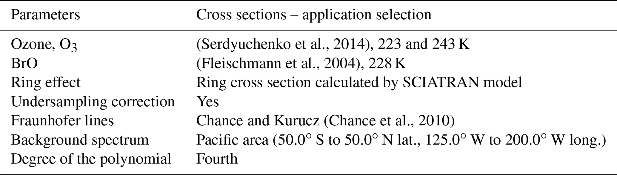
where b_p represents the coefficients of the polynomial. Variants on Eq. (4) are also employed to fit the spectra. To retrieve accurate BrO SCDs, an optimal selection of the spectral window, which maximizes the information content with respect to the BrO absorption, and the selection of corresponding cross sections of other trace gases absorbing in the same spectral window are the first step. We chose to use temperature-dependent cross sections of ozone (dominant absorber in the UV) following Serdyuchenko et al. (2014) at 223 and 243 Kelvin and a BrO cross section (Fleischmann et al., 2004) at 223 Kelvin. In addition, a pseudo-cross section is used for simulating the filling in of Fraunhofer lines by Raman scattering known as the Ring effect (Vountas et al., 1998), and another pseudo-cross section, which deals with the issue of poor spectral sampling (Chance et al., 2005), was included in the fitting for all instruments. The high-spectral-resolution absorption cross sections were convolved by the slit function of each instrument. The impact of using different combinations of trace gas absorptions on the fit of BrO SCD was investigated. It was found that the omission of the explicit fitting of NO₂ and SO₂ has a minimal impact on the fit of the BrO SCD north of 70^∘ N. The differences in BrO SCD between fits with and without NO₂ or SO₂ in the selected spectral ranges were typically less than 1 % of the BrO SCD. Consequently, we decided to use only the cross sections of the dominant absorber O₃ in this region and of the trace gas of interest itself, BrO, in the nonlinear least squares SCD fitting. The differences between fits of BrO SCD using fourth- and fifth-order polynomials were small and the quality of the fit improved significantly from a third- to fourth-degree polynomial fit. These results led to the selection of the use of the fourth-order polynomial in our retrieval. The selection of parameters used in this study is appropriate for BrO columns in the region north of 70^∘ N.

As BrO is a relatively weak absorber, small changes in the input parameters and especially of the fitting window of the retrieval lead to large changes in the quality of the fit. Although there are many good practices developed for the DOAS fitting window selection for an absorber (e.g., it must include at least two absorption peaks from the trace gas of interest, no large Fraunhofer lines, small interference from other species, etc.), there is no precise and agreed methodology to determine the optimal selection. Consequently, different spectral fitting windows for BrO retrievals have been used in previous studies. For example, Richter et al. (1998) used a 345–359 nm wavelength region for GOME, Afe et al. (2004) used a 336–347 nm fitting window for SCIAMACHY and Theys et al. (2009) used a 336 to 359 nm fitting window for GOME-2A. Each of the sensors has slightly different instrumental characteristics, and each of them shows different degradation behavior. Consequently, we chose the optimal spectral fitting window for each of the sensors using the following set of selection criteria: (a) smallest root mean square error (RMSE) of the fit; (b) minimal trend of BrO SCDs over a clear Pacific reference region, where no strong trend in BrO is expected; and (c) good agreement between retrievals from the different sensors for periods of overlapping measurements. The RMSE of the fit in absolute units is defined as where N is the number of spectral points and P(λ) the low-order polynomial. The RMSE was averaged over all the scenes in the region of interest (i.e., the Arctic from 70.0 to 85.0^∘ N latitude and 180^∘ W to 180^∘ E longitude) and for the Pacific reference region (50.0^∘ S to 10.0^∘ N latitude and 90.0 to 125.0^∘ W longitude).

Figure 1 shows the SCDs of BrO over the Pacific reference region and the RMSE of the fit for the Arctic and Pacific regions.

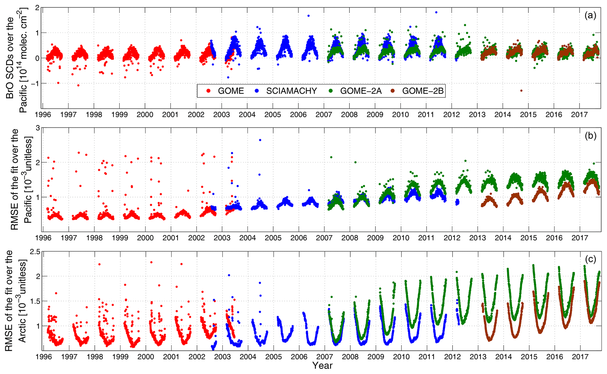
Figure 1 Time series of (a) SCDs of BrO (molec cm⁻²) over the Pacific, (b) fitting RMSE over the Pacific and (c) fitting RMSE over the Arctic. GOME data are shown in red, SCIAMACHY in blue, GOME-2A in green and GOME-2B in brown color.

The annual cycle in the fitting RMSE for the Arctic results from changes in the Sun's position and its impact on the upwelling radiance. In spring and autumn, when the solar zenith angle is larger, the scattering and attenuation increases, and as a result, the radiance signal is low. In the Arctic, SCIAMACHY has the lowest fitting RMSE of all instruments. GOME-2A shows a rapid increase in RMSE up to 2009 and a smaller upward trend in the following years. A similar systematic increase in RMSE occurs for GOME-2B. The RMSE for the Pacific region shows a similar behavior for GOME-2A and GOME-2B, as both increase strongly with time. GOME appears to have lower RMSE values on average than the GOME-2A and GOME-2B instruments, presumably because of the lower spatial resolution, but the RMSE shows large variability. Generally, daily mean RMSE values are below $\mathrm{2.0}\times {\mathrm{10}}^{-\mathrm{3}}$, for all instruments. There is no clear trend in the SCD of BrO over the Pacific region for any of the instruments.

The use of a reference area over the Pacific as background spectrum is an alternative to the use of solar irradiance measurements, which removes systematic errors arising from interfering instrumental structures in the solar irradiance measurements. The region of the Pacific is selected because of its relatively small annual cycle of BrO (Richter et al., 2002). In this way, the quality of the fit improves greatly as problems in the radiances mainly cancel out. Consequently, the Pacific background spectrum has been used instead of the Sun background spectrum for all instruments in the present study. Although trends over the clean Pacific background region resulting from instrumental degradation were minimized, residual trends had to be accounted for. This has been achieved by applying an additional Pacific correction to each instrument separately. The normalization method computes the average BrO SCD in a small Pacific area ($\mathrm{0.0}{}^{\circ }\pm \mathrm{10.0}{}^{\circ }$ latitude, $\mathrm{180.0}{}^{\circ }\pm \mathrm{20.0}{}^{\circ }$ longitude) and then subtracts this average from every pixel of the BrO SCD. To compensate for the negative bias imposed by the method, a constant offset of 7×10¹³ molec cm⁻² was added for every day (Richter et al, 2002; Sihler et al., 2012). This correction tackles offset errors that occur for weak absorbers and are due to instrumental degradation (Alvarado et al., 2014).

The empirically determined sets of parameters used in the BrO retrievals are reported in Tables 2 and 3.

Table 2 Parameter selection for all instruments.

3.2 Tropospheric BrO vertical column densities and datasets

NO₂ and O₃ columns from satellite retrievals and tropopause height from meteorological reanalysis data are used for extracting the tropospheric BrO component from the retrieval (stratospheric separation). Sea ice data (age and type) obtained by satellite remote sensing were used in order to identify regions with sea ice cover and hence high surface reflectivity, which is required for the retrieval of tropospheric BrO in this study and for data interpretation in relation to bromine sources.

3.2.1 Stratospheric separation

In order to derive the tropospheric BrO VCD from the retrieved SCD of BrO, the method of Theys et al. (2009) was used. Briefly, this method uses a stratospheric BrO climatology, derived with the BASCOE model (Errera and Fonteyn, 2001), and requires year, latitude, tropopause height, O₃ and NO₂ columns as input. This approach has been applied successfully in previous studies (e.g., Begoin et al., 2010; Theys et al., 2011; Blechschmidt et al., 2016; Choi et al., 2018). In the present study, satellite-retrieved O₃ VCDs from Weber et al. (2013), stratospheric NO₂ VCDs from the QA4ECV project (Boersma et al., 2017a, b, c) and from the Tropospheric Emission Monitoring Internet Service (TEMIS) (Boersma et al., 2004), and tropopause heights retrieved from NCEP reanalysis data (Kalnay et al., 1996) were used as input. In Theys et al. (2009), a correction factor was applied to account for the long-term reduction of bromine emissions in the stratosphere. This factor was based on ground-based zenith-sky measurements of BrO over Harestua (Hendrick et al., 2008). In the present study, this factor was excluded, as the long-term development of stratospheric BrO VCDs of the model without applying the correction factor comes to a closer qualitative agreement with updated measurements of BrO over Harestua (from F. Hendrick, BIRA-IASB, personal communication, 2019). The time series of NO₂, O₃ and tropopause height are shown in Fig. 2.

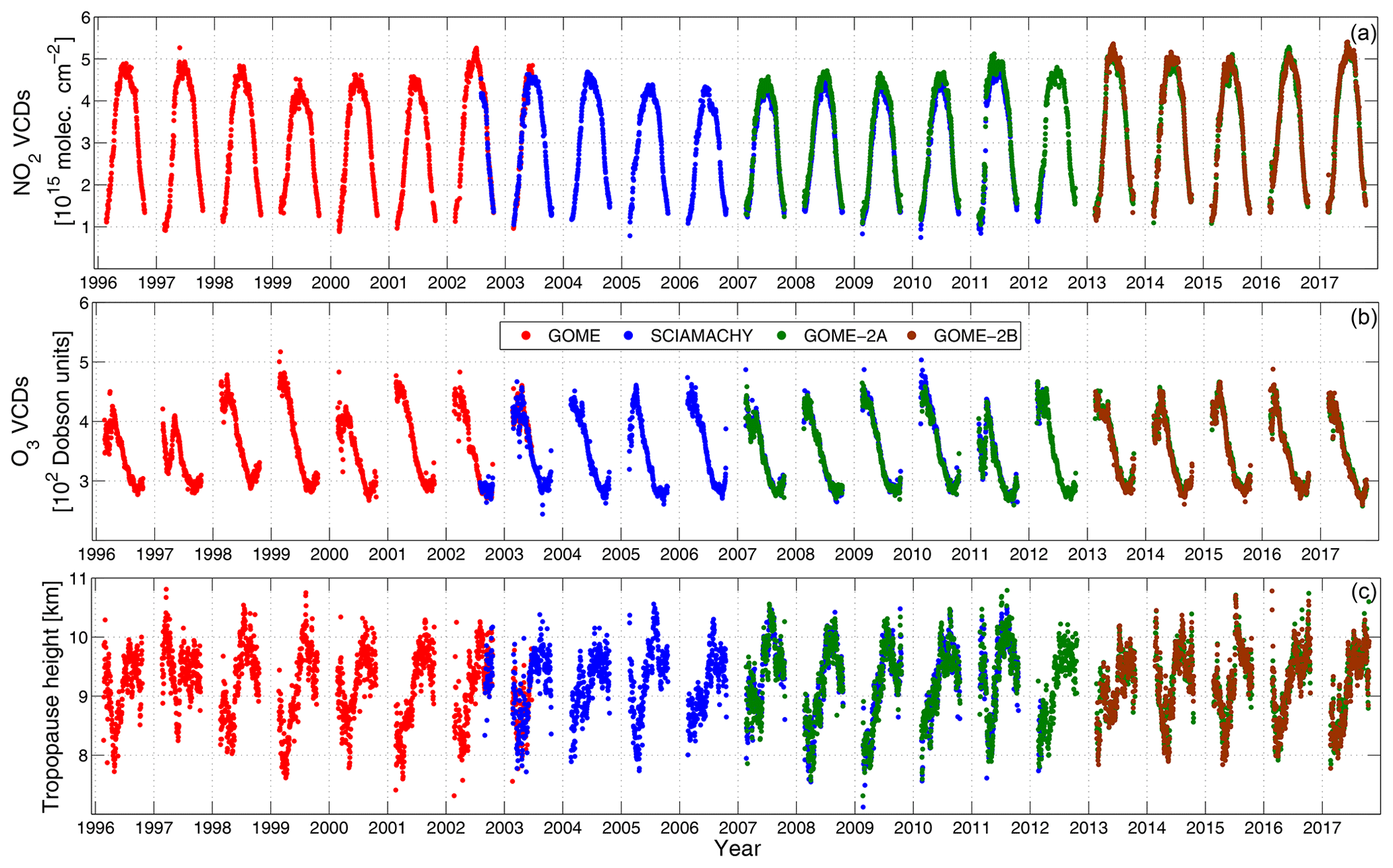
Figure 2 Time series of daily averaged input data over the Arctic used for deriving stratospheric BrO VCDs: (a) stratospheric NO₂ VCDs (molec cm⁻²) from QA4ECV (GOME, SCIAMACHY and GOME-2A) and TEMIS (GOME-2B), (b) O₃ VCDs (Dobson units) from Weber et al. (2013), and (c) tropopause height (km) from NCEP reanalysis data. Data for the GOME instrument are colored in red, SCIAMACHY in blue, GOME-2A in green and GOME-2B in brown. All three time series show daily averages over the Arctic region (>70^∘ N).

The following formula (Theys et al., 2009) is used to derive the tropospheric VCD of BrO:

$$\begin{array}{}\text{(5)}& {\mathrm{\text{VCD}}}_{\text{tropo}}=({\text{SCD}}_{\text{total}}-{\text{VCD}}_{\text{strato}}\times {\text{AMF}}_{\text{strato}})/{\text{AMF}}_{\text{tropo}},\end{array}$$

where SCD_total is the slant column of BrO retrieved by the DOAS method, VCD_strato corresponds to the stratospheric BrO VCD retrieved from the Theys et al. (2009) climatology, AMF_strato is a stratospheric air mass factor and AMF_tropo is a tropospheric air mass factor. For the latter, as in Begoin et al. (2010) and Blechschmidt et al. (2016), a surface albedo of 0.9 has been assumed above sea ice and that all tropospheric BrO is well mixed within the boundary layer extending to 400 m altitude. Note that the stratospheric BrO VCD column is independent of the BrO SCD and only depends on the Theys et al. (2009) climatology and its inputs.

3.2.2 Sea ice

In order to study the connection between tropospheric BrO and sea ice under the impact of Arctic warming, long-term sea ice data (starting from 1996) are required in this study. In addition, since the tropospheric AMF applied for the retrieval of tropospheric BrO (see previous section) assumes a surface albedo of 0.9, the sea ice data were used to remove data with no sea ice cover from the BrO data. For this purpose, the sea ice age dataset from Tschudi et al. (2019) was used. It is retrieved from different passive microwave satellite remote sensing instruments and has a very high spatial resolution of 12.5 km×12.5 km, while its temporal resolution is 7 d.

4 Results

The passive remote sensing spectrometers GOME, SCIAMACHY, GOME-2A and GOME-2B measure the upwelling reflectance at the top of the atmosphere. The months of October to February have few or no observations due to polar night in the target latitudes north of 70.0^∘ N. The largest solar zenith angle (SZA) used is 80^∘. The long-term analysis of BrO columns was performed during the period from March until September, from 1996 to 2017. This period has the best coverage by the ultraviolet–visible (UV–VIS) satellite remote passive sensors at high latitudes. The analysis is restricted to data northwards of 70.0^∘ N, which is referred to as the Arctic. This region was chosen because the source regions of bromine explosions and thus plumes of elevated BrO are known to be associated with regions of sea ice cover. We present the derived BrO VCD time series for the Arctic region, together with corresponding annual cycles, scatterplots and map plots in Sect. 4.1. The tropospheric BrO is correlated with sea ice coverage and age in Sect. 4.2 to investigate the impact of changing sea ice conditions on BrO amounts in the Arctic's troposphere. Finally, a trend analysis of tropospheric BrO is performed together with a check for statistical significance of the trends (Sect. 4.3).

Table 3 Fitting windows used for the different instruments.

4.1 Comparison between the BrO columns retrieved from different sensors

The geometric BrO VCD is retrieved by dividing the BrO SCD with a simple stratospheric AMF, which takes into account the scattering at the surface but ignores the impact of scattering within the atmosphere. Consequently, it necessarily differs from the sum of the tropospheric and stratospheric column. Daily values of the geometric, stratospheric and tropospheric VCDs of BrO over the Arctic region are shown in Fig. 3.

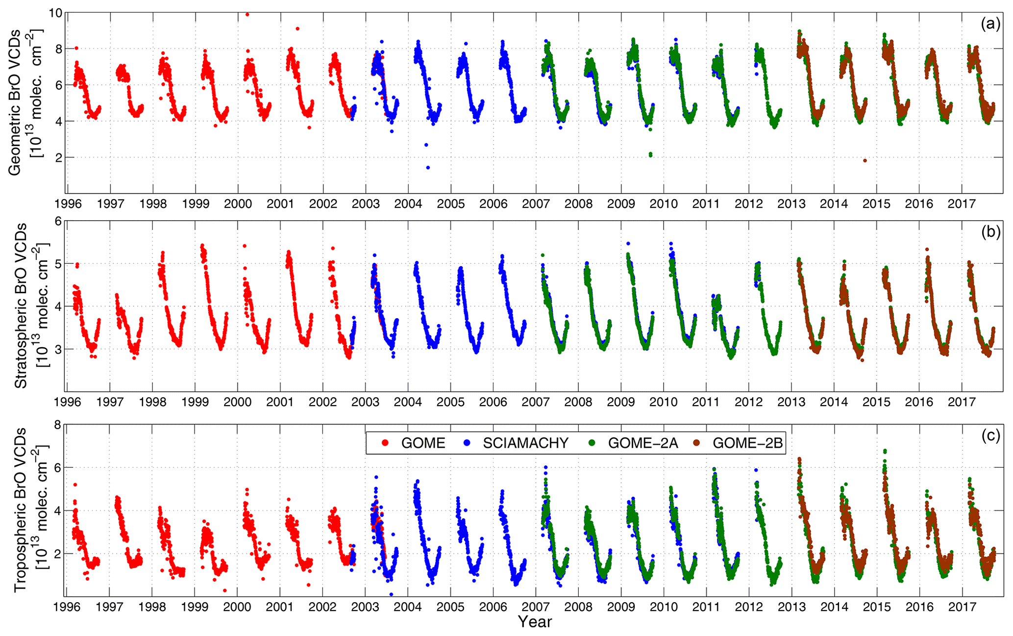
Figure 3 Long-term BrO time series over the Arctic region: (a) daily geometric BrO VCDs (10¹³ molec cm⁻²), (b) daily stratospheric BrO VCDs (10¹³ molec cm⁻²) and (c) daily tropospheric BrO VCDs (10¹³ molec cm⁻²). All figures show daily averages ≥ 70.0^∘ N. GOME data are colored in red, SCIAMACHY in blue, GOME-2A in green and GOME-2B in brown.

The geometric VCD accounts for the expected differences between the different viewing geometries of the satellite sensors to a good first order. There is good agreement during periods of overlapping measurements, e.g., between the retrieved geometric BrO VCD from GOME and SCIAMACHY (from August 2002 to June 2003), SCIAMACHY and GOME-2A (from March 2007 to March 2012), and finally GOME-2A and GOME-2B (from March 2013 to September 2017). A quantitative comparison is provided below. The stratospheric BrO VCDs show a small upward trend from 1995 to 2001 and a slight decrease afterwards, which are in agreement with measurements of stratospheric BrO from Harestua station (Hendrick et al., 2008).

The comparison of tropospheric BrO VCD time series during the periods of overlap between the different instruments shows a similar level of agreement to that of the geometric VCDs. The seasonality of the tropospheric time series is also similar to the geometric one. We attribute this seasonality to be in large part a result of the inorganic release of Br₂ and BrCl from sources, which depend on sea ice and meteorological parameters. As described in the introduction, in polar spring, the combination of low-temperature conditions on first-year sea ice, having sufficient brine, triggers the release of Br₂ and BrCl into the troposphere. This condition prevails in spring, moving slowly northwards with the solar zenith angle. During July and August, the temperature reaches its maximum. In September, the minimum sea ice extent is observed. The release of organobromine compounds from the oceanic biosphere is hence expected to be highest in summer and early autumn. This provides a biogenic source of bromine, but the oxidation of organic-bromine-containing compounds is relatively slow compared to the release of BrO from bromine explosion events. During summer and early autumn, tropospheric BrO VCDs reach their minimum values of the year. A small increase is observed in each September. The origin of this increase is not yet identified. Potential candidate explanations include inaccuracies in the stratospheric BrO VCD calculation or potentially lower temperature accelerating the inorganic release of bromine from brine without reaching the threshold for explosion.

We identify peaks in the tropospheric BrO VCD time series: 2007, 2013 and 2015 are the years with the highest tropospheric BrO VCDs in polar spring. Hollwedel et al. (2004) investigated the period from 1996 to 2001. Despite the different settings and cross sections used in the retrieval, their geometric VCDs have similar magnitudes and patterns to those presented here (i.e., they increase from 1997 to 1998 and then decrease from 1999 to 2000). It is also interesting to compare the results from this study with those from Choi et al. (2018). They used the operational product of the OMI (from 2005 to 2015) and the same stratospheric separation method as applied here. In agreement with our findings, Choi et al. (2018) found a peak in tropospheric BrO VCDs in 2007. However, the OMI dataset does not show the same increase as the SCIAMACHY and GOME-2A data in later years. The origin of this difference is not identified. It may be due in part to the strong row anomaly affecting the OMI data product (Class et al., 2010).

Figure 4 shows scatterplots of geometric and tropospheric VCDs for the three overlapping time periods of the instruments.

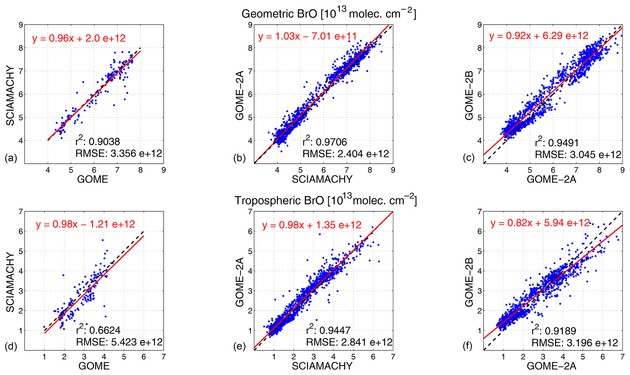
Figure 4 Scatterplots of (a, b, c) geometric BrO VCDs and (d, e, f) tropospheric BrO VCDs for (a, d) GOME against SCIAMACHY (August 2002 to June 2003), (b, e) SCIAMACHY against GOME-2A (March 2007 to March 2012) and (c, f) GOME-2A against GOME-2B (March 2013 to September 2017). The dashed black line in each scatterplot is the reference line, and the red one is the linear regression line. The Pearson correlation coefficient (squared, r²), the RMSE and the y function of the regression line are also given. The units for all scatterplots are (10¹³ molec cm⁻²).

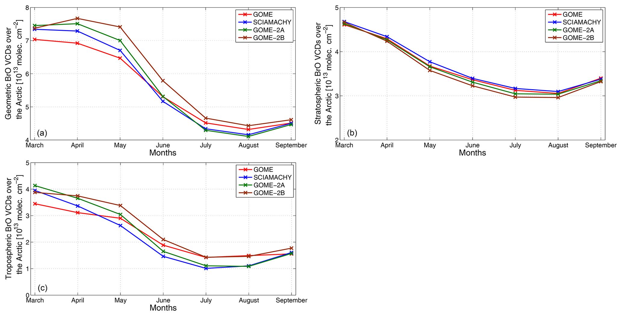
Figure 5 Climatological seasonal cycles of (a) geometric BrO VCDs (10¹³ molec cm⁻²), (b) stratospheric BrO VCDs (10¹³ molec cm⁻²) and (c) tropospheric BrO VCDs (10¹³ molec cm⁻²) over the Arctic for GOME (red), SCIAMACHY (blue), GOME-2A (green) and GOME-2B (brown).

The best agreement is found between SCIAMACHY and GOME-2A, both for the geometric and the tropospheric VCDs, while the agreement is poorer between GOME and SCIAMACHY (this is attributed to the comparably short overlapping period between these sensors).

Climatological seasonal cycles (averages over the whole period of retrievals of geometric, stratospheric and tropospheric VCDs) for each instrument are shown in Fig. 5.

The annual cycles of the geometric and the tropospheric VCD time series are similar in shape. The largest VCDs occur for all instruments in polar spring (March to May), followed by a strong decrease from May to June. In spring, GOME-2B VCDs are slightly larger, while GOME columns are slightly lower than data from the other instruments for the geometric VCDs. In summer and early autumn GOME VCDs are higher. For the tropospheric VCDs, the differences between the instruments become smaller.

Figure 6 shows average maps of geometric VCDs of BrO over the Arctic for the overlapping periods of the sensors.

Retrieved geometric BrO VCDs occur in similar locations and are of similar magnitude to the different instruments. A qualitative comparison of geometric BrO VCDs between this study and the one by Hollwedel et al. (2004) shows good agreement, with plumes of BrO being of similar magnitude and appearing over the same locations.

Figure 7 shows the evolution of tropospheric BrO VCD maps over the Arctic over 4 d of selected bromine explosion events – one event for each overlap period of the different sets of sensors.

Bromine explosion events are characterized by high values of tropospheric BrO VCDs, which occur every polar spring. The agreement between the tropospheric BrO VCDs retrieved from the different sensors is good, as shown above. BrO plumes appear over the same areas and have similar magnitudes for each bromine explosion case. The times of observations are similar but not identical, and we have not identified evidence of this influencing the comparison of tropospheric BrO VCDs. The sensors also observe the transport of plumes of BrO by cyclones away from the initial release area (e.g., the 2007 case shown in Fig. 5, investigated in more detail by Begoin et al., 2010). Hence, the track of cyclones transporting BrO plumes is expected to influence longer-term averaged BrO maps.

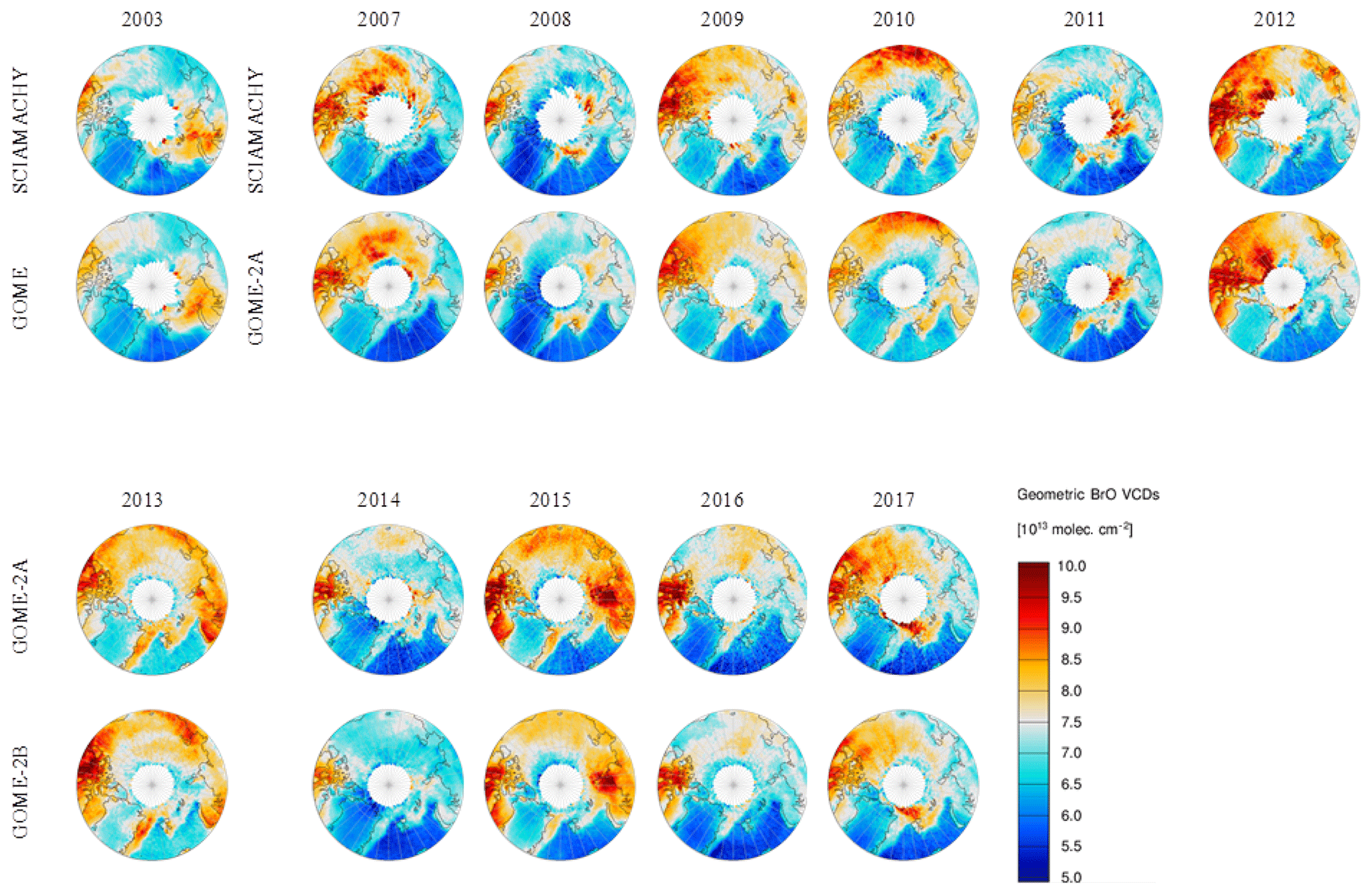
Figure 6 Monthly mean for March of geometric BrO VCDs (10¹³ molec cm⁻²), in the Arctic region. Rows indicate different instruments, while columns indicate different years of overlapping periods of measurements.

4.2 Arctic tropospheric BrO and its relationship to sea ice

In this section, the evolution of tropospheric BrO and its relation to sea ice is presented. More specifically, the relationship between first-year ice and tropospheric BrO is investigated. Since an albedo of 0.9 was assumed in the tropospheric AMF, a sea-ice-based ground scene flagging of our tropospheric BrO dataset was performed. In this way, only BrO observations above sea ice are analyzed. BrO plumes are also transported over the ocean, but in this study, we focus on the plumes created by bromine explosions over sea ice. As described in Sect. 4.1, the individual BrO VCD time series from the four sensors are highly consistent, and the remaining inconsistencies are small. Hence, a merged tropospheric BrO dataset over sea ice was retrieved by averaging the overlapping days between the sensors. The merged tropospheric BrO VCD dataset is shown in Fig. 8 together with the results from the individual sensors and the time series of sea ice extent from Tschudi et al. (2019).

Figure 7 Examples of bromine explosion events over the Arctic region for overlapping measurement periods between the sensors. Rows refer to the different instruments, whereas columns refer to the dates. For each case, four daily average maps of tropospheric BrO VCD (10¹³ molec cm⁻²) are shown.

By comparing Figs. 8b and 3c, it is found that bromine explosion events are becoming more evident (for example in years 2007 and 2015) if we apply the sea ice flagging (i.e., keeping only scenes with sea ice coverage).

In order to investigate the spatial evolution of tropospheric BrO in time and its relationship to sea ice age, polar spring (March to May) average maps of tropospheric BrO and corresponding sea ice age maps are displayed in Fig. 9 for each year between 1996 and 2017.

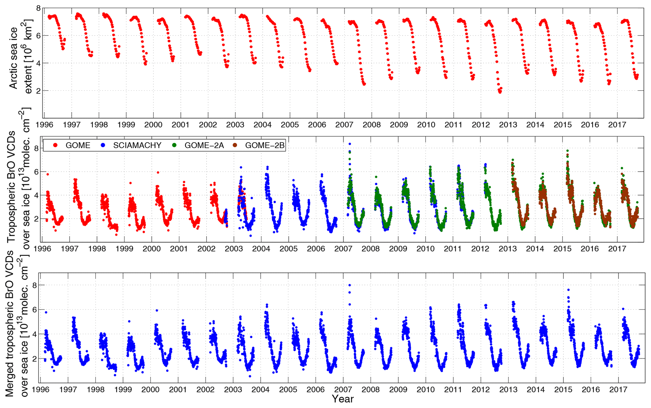
Figure 8 (a) Arctic sea ice extent from March until September from Tschudi et al. (2019); (b) tropospheric BrO VCDs above sea ice in the Arctic (GOME data are shown in red, SCIAMACHY in blue, GOME-2A in green and GOME-2B in brown); and (c) the sensor merged tropospheric BrO VCDs above sea ice in the Arctic.

In the past two decades, the area covered by multiyear ice has decreased, and that covered by first-year ice has increased. The elevated levels of BrO are predominantly found over first-year ice. The magnitude of the elevated BrO plumes has generally increased, with the maximum occurring in the years 2013 to 2015. In addition, the area in which bromine explosion events occur in the March to May period has changed over the years. For example, from 2010 and onwards, BrO is formed at the eastern coastline of Greenland comparatively at lower latitudes and inside the Arctic Ocean at higher latitudes (larger than 80.0^∘ N), something not evident in the early years (i.e., 1996 to 2001). In addition, from 2001 to 2003, most of the BrO is found in the region of the Barents and Kara Sea (to the north of Scandinavia and Russia). However, from 2009 onwards, BrO plumes have spread over the Arctic region.

Figure 9 Polar spring (March, April and May, MAM) averages of tropospheric BrO VCDs (10¹³ molec cm⁻²) over sea ice, compared to sea ice age in the Arctic. Columns refer to years, odd rows to tropospheric BrO VCDs and even rows to sea ice age.

First-year ice has become more dominant over the Arctic region in recent years (i.e., 2009 onwards). The year 2009 was the first year for which large tropospheric BrO VCDs were evident over the Canadian Arctic Archipelago and the Beaufort Sea. In 2009, the area of multiyear ice decreased significantly in these regions. Similarly, the appearance of BrO plumes over the northwest coast of Greenland in 2015 is in agreement with the appearance of first-year ice during this year. The relationship between first-year ice and BrO VCD is not straightforward or linear but apparent in all years. We attribute the behavior to BrO sources, conditions at the surface of potential frost flowers, blowing snow and cold brine, and the transport of air masses in which bromine explosions are occurring. In 2004, for example, the highest BrO VCDs are found over a multiyear ice area, whereas in 2002 BrO is mainly seen over first-year ice. The increase in magnitude of BrO plumes is not simply related to the development of first-year ice as identified in the maps above. In summary, the increase in the areas where tropospheric bromine explosions occur is related in a nonlinear way to the increase in first-year-ice-covered Arctic regions.

Figure 10 shows yearly anomaly polar spring maps of tropospheric BrO VCDs with respect to the 22-year mean. The 22-year average is shown in the last row of the figure.

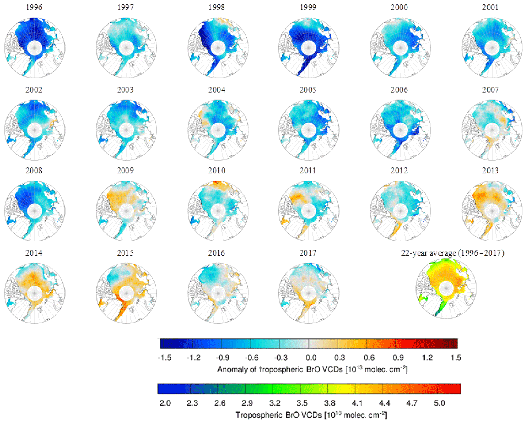
Figure 10 Anomaly maps of polar spring (MAM) tropospheric BrO VCDs (10¹³ molec cm⁻²) over sea ice. From every MAM average, the 22-year average (1996 to 2017, shown at the bottom right of row four) of tropospheric BrO VCDs was subtracted.

During the first years of the time series, BrO VCDs are lower than on average in most regions of the Arctic. The first large positive anomaly compared to the mean occurs in 2009 and in areas where first-year ice appeared for the first time.

From 2011 onwards, BrO VCDs grow in the north and to the east of Greenland. When comparing the last with the first 5 years of the time series, BrO VCDs have increased.

Figure 11 shows plots that probe the relationship between tropospheric BrO and first-year ice extent. More specifically, Fig. 11a shows a plot of the polar spring tropospheric BrO VCD above first-year ice and first-year ice extent, and Fig. 11b shows the area of ice where the tropospheric BrO VCD exceeds a threshold of 7×10¹³ molec cm⁻². This threshold value was chosen empirically, as in previous studies (Hollwedel et al., 2004; Choi et al., 2018). First-year ice extent and corresponding scatterplots are also given. For the time series of this figure, all the polar spring values north of 70^∘ N for each year were averaged, thereby deriving one value per year.

Figure 11 (a) Polar spring (MAM) mean time series of tropospheric BrO VCDs over sea ice and first-year sea ice extent over the Arctic, (b) polar spring (MAM) mean time series of areas with BrO VCDs above the threshold of 7×10¹³ molec cm⁻² and first-year sea ice extent over the Arctic, (c) scatterplots showing polar spring averages of tropospheric BrO VCDs against first-year ice extent, and (d) polar spring averages of areas with tropospheric BrO VCDs exceeding the threshold of 7×10¹³ molec cm⁻² against first-year ice extent in the Arctic. The linear regression lines in (c) and (d) are shown in red in each scatterplot. The Pearson correlation coefficient (r), its error and the root mean square errors (RMSE) between the regression line and plotted quantities are shown in each scatterplot.

The total Arctic sea ice extent has decreased over the last years, but the area covered by first-year sea ice has increased. The type of ice encountered at the surface is changing. Due to the increasing temperatures in the Arctic, more sea ice now melts every year, and more first-year or young sea ice is formed each winter period. Figure 11a shows that 2008 was the first year that first-year ice extent exceeded the threshold of 5×10⁶ km², which is also the case for almost all of the following years. The first-year ice extent in spring (i.e., the area of first-year ice in the months March until May) for the decade 2007 to 2017 is larger than that from 1996 to 2006. Although tropospheric BrO VCDs have also increased in magnitude approximately from 2007 onwards, BrO VCD and sea ice area do not correlate strongly. In the years 2008 and 2016, a decrease in tropospheric BrO VCDs, when compared to 2007 and 2015, respectively, is found, while first-year ice extent increased. In 2015, the highest tropospheric BrO VCD polar spring averages are found. In the same year, the polar spring first-year sea ice extent average has its lowest value after 2008. Similar conclusions can be drawn from Fig. 11c. Although most days of average BrO above 7×10¹³ molec cm⁻² are occurring with first-year ice extent above 4.5×10⁶ km², we can see such days also below this threshold. The positive correlation coefficient between polar spring tropospheric BrO VCDs and first-year sea ice extent for the same period is 0.32 with an error of 0.021. The significance of the correlation was verified by performing a significance test, based on the p values. The null hypothesis (there is no correlation between the two quantities) was rejected, as the p value was <0.05. Therefore the significance test was successful, meaning there is a correlation between tropospheric BrO and sea ice age (although, based on the actual value of the correlation coefficient, it is moderate). The correlation between areas of enhanced tropospheric BrO VCDs and first-year ice extent is lower, approximately 0.2 with an error of 0.022. This is evident from both the time series (Fig. 11b) and their scatterplot (Fig. 11d, bottom right). In this case, the significance test was not successful, i.e., there is not a correlation between areas of BrO VCDs $>\mathrm{7}\times {\mathrm{10}}^{\mathrm{13}}$ molec cm⁻² and first-year ice extent. We have also calculated correlation coefficients for the annual time series (Fig. 11a and b). In this case, the correlation coefficient between tropospheric BrO VCDs and sea ice extent is 0.62 and for the area of BrO VCDs $>\mathrm{7}\times {\mathrm{10}}^{\mathrm{13}}$ molec cm⁻² and first-year ice extent 0.46. However, since these calculations are based on only 22 values, they are statistically less important than the correlation coefficients calculated based on the daily time series. It seems that, in both cases, the largest number of days with high tropospheric BrO VCDs or largest areas of bromine explosion events are occurring when first-year ice extent is between 4.5×10⁶ and 5×10⁶ km² and not when it reaches its peak. The magnitude of tropospheric BrO VCDs is positively and significantly but not strongly related to first-year ice extent. This conclusion is consistent with a strongly nonlinear bromine explosion mechanism dependent on more than one key parameters. This finding is in contrast to the results by Choi et al. (2018), where an analysis of BrO VCD retrieved from the OMI was performed. They found a correlation coefficient of −0.32 between first-year ice extent and tropospheric bromine explosion frequency. The negative sign is attributed to a decrease in tropospheric BrO VCDs over the latter years of the trend analysis. The differences to Choi et al. (2018) may be explained by a degradation of the OMI (Kroon et al., 2011).

4.3 Trend analysis

A trend analysis of the tropospheric BrO VCD time series is performed in order to investigate the statistical significance of the observed temporal and spatial changes in tropospheric BrO VCDs associated with the Arctic warming. The tropospheric BrO VCD time series shows a seasonality, with a maximum every polar spring (March in most cases) and a minimum every summer. Consequently, a model which combines a linear trend and seasonal variations is selected, similar to that used in previous studies (Hendrick et al., 2008; Georgoulias et al., 2019). We calculated trends using Eq. (7):

$$\begin{array}{}\text{(6)}& \mathrm{d}\left(t\right)=At+B+\sum _{i=\mathrm{1}}^{\mathrm{3}}\left\{C_i\cos \left({\displaystyle \frac{\mathrm{2}\mathit{\pi }}{M}}\left(t\right)\right)+D_i\sin \left({\displaystyle \frac{\mathrm{2}\mathit{\pi }}{M}}\left(t\right)\right)\right\},\end{array}$$

where A is the slope, B is the intercept, d(t) is the modeled value of BrO VCD on a given day, t is the day of the dataset (expressed in fractional years) and M is the period in years. The number of harmonic functions was chosen based on the minimization of the residuals between the model and the dataset. The error of each trend was calculated using Eq. (8) (Weatherhead et al., 1998):

$$\begin{array}{}\text{(7)}& {\mathit{\sigma }}_B=\left[{\displaystyle \frac{{\mathit{\sigma }}_M}{M^{\mathrm{3}/\mathrm{2}}}}\sqrt{{\displaystyle \frac{\mathrm{1}+\mathit{\phi }}{\mathrm{1}-\mathit{\phi }}}}\right],\end{array}$$

where σ_M is the standard deviation of the residuals between the model and the time series, M is the period in years, and φ is the autocorrelation of the residuals (0.2). Finally, a trend is considered significant if the ratio between it and its error is greater than 2 (Weatherhead et al., 1998).

Table 4 shows the trends of tropospheric BrO over sea ice north of 70^∘ N over the whole period (see Fig. 8c), for individual months and for the area of the BrO VCD associated with bromine explosions (Fig. 11b). For the trends of the individual months, we did not use the trend model with harmonics in Eq. (7) and used Eq. (9) instead:

$$\begin{array}{}\text{(8)}& \mathrm{d}\left(t\right)=At+B.\end{array}$$

Table 4 Trends of tropospheric BrO VCD (over the whole period and for individual months) and for the area of plumes from bromine explosions between 1996 and 2017, together with their errors and significance of each trend. The unit for all quantities is molecules per square centimeter (molec cm⁻²), except the for the area of BrO plumes (km²).

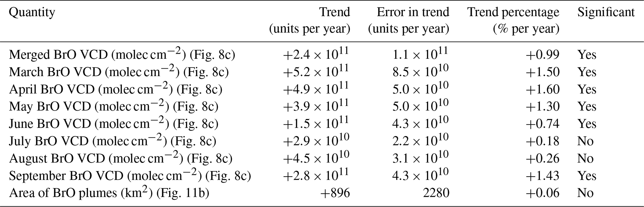
The monthly trends in Table 4 with the exception of the trends of the summer months July and August and for the trend of BrO plumes are statistically significant. The linear trend of the annual tropospheric BrO VCD over the Arctic shows an approximately 1 % increase per year over the last 22 years. During individual polar spring months the increase in BrO VCD is stronger, reaching a value of 1.5 % yr⁻¹. The trends of BrO VCD during summer months are smaller, and those in July and August are statistically insignificant.

Figure 12 shows the trends appearing in the tropospheric BrO time series, based on different time periods, i.e., different starting and ending years. Equation (9) was used to calculate the trends, starting from and to the same date for both the starting and the ending years (i.e., end of March).

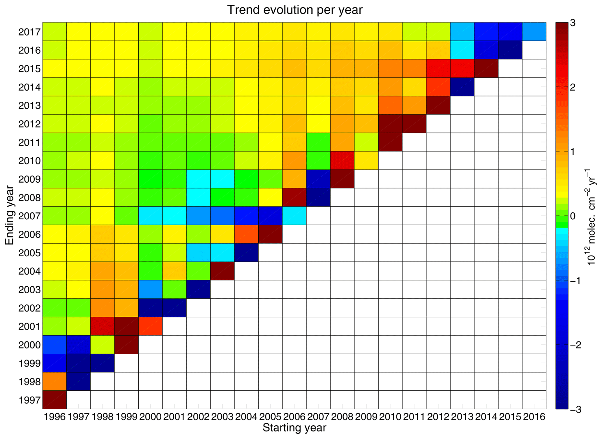
Figure 12 Trend (10¹² molec cm⁻² yr⁻¹) evolution of the merged tropospheric BrO dataset (i.e., slope of the linear regression line) over sea ice. The x axis shows the starting year and the y axis shows the ending year of the period over which the trend was calculated.

Linear trends calculated by starting in one year and ending in the next one (e.g., from 1996 to 1997) are in agreement with the BrO VCD shown in Fig. 8c (for example, the strong positive change from 2014 to 2015 or the decrease from 1997 to 1998). Trends over short periods are dominated by interannual variability. The positive linear trends are largest when the later years are included. We see that the strongest long-term positive trends occur when we choose as a starting point the years 2006–2008 and as an ending point the year 2017.

In Fig. 13, the trend for each individual grid box during polar spring months is displayed for tropospheric BrO, sea ice age and first-year ice frequency occurrence. All three maps are gridded in $\mathrm{0.125}{}^{\circ }\times \mathrm{0.125}{}^{\circ }$ resolution. The trend for every grid box is calculated using Eq. (9).

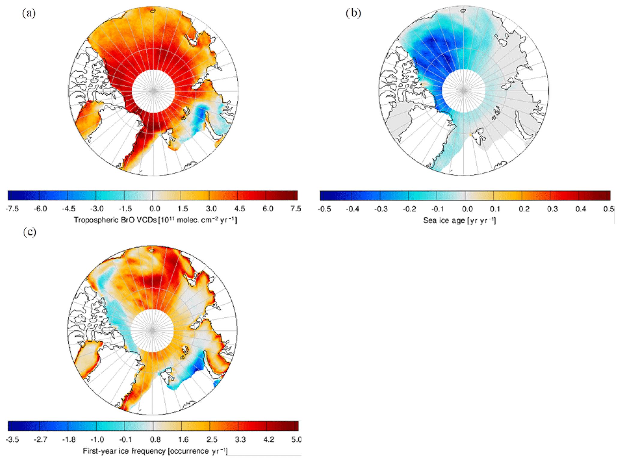
Figure 13 Polar projection of the trend in each grid box ($\mathrm{0.125}{}^{\circ }\times \mathrm{0.125}{}^{\circ }$) during polar spring months (March, April, May, MAM) for (a) tropospheric BrO VCD over sea ice (10¹¹ molec cm⁻² yr⁻¹), (b) sea ice age (years per year) and (c) first-year ice frequency (occurrence per year). The trends calculated over a 22-year period (1996 to 2017).

Tropospheric BrO VCD values increase inside the region of the Arctic Ocean and also to the north and east of Greenland, where sea ice age shows negative trends. We learned from Fig. 9 that, after 2008, first-year ice appears in the same area. This can also be verified by Fig. 13c, as in the same area we see a positive increase of 2.5 to 3 first-year ice occurrences per year. However, the trends of tropospheric BrO VCD and sea ice age do not match everywhere. The strongest negative trends in the sea ice map occur in areas where multiyear ice was dominant in the past, and first-year ice has formed in the recent years (Beaufort Sea and Canadian Arctic Archipelago). However, in the same area, we do not see the most pronounced increase in the trend map of tropospheric BrO VCDs (the increase is smaller than in other areas). The strongest increase in tropospheric BrO VCDs occurs to the northeast of Greenland close to the Fram Strait, to the north of Greenland and close to Ellesmere Island. Although first-year ice seems to be appearing more frequently in the east of Greenland, we do not see the same evolution on the north side of Greenland. On the contrary, we see a decrease in first-year ice occurrences over the latest years. Therefore, we can conclude that, although first-year ice has a relation to the increased tropospheric BrO plumes observed over the recent years, it is not the only parameter affecting the formation of enhanced BrO.

5 Summary and conclusions

In this study, a merged dataset of tropospheric BrO VCD over the Arctic north of 70^∘ N retrieved from the measurements of four similar UV–VIS remote sensing satellite instruments over a 22-year time period is presented. A high level of consistency of the retrieved BrO VCDs was found between the retrievals from the different sensors. Time series of tropospheric BrO VCDs over the Arctic north of 70^∘ N and corresponding trends indicate that the magnitude of tropospheric BrO VCDs has increased, especially in the decade from 2007 to 2017, when we observe a 1.23 times stronger increase than from the period 1996 to 2017. This increase is pronounced in polar spring, when the majority of bromine explosion events occur. Additionally, from the spatial patterns of tropospheric BrO VCD, we infer that the size of the areas of elevated BrO VCD (i.e., impacted by bromine explosions) has increased about 896 km² yr⁻¹.

The correlation between tropospheric BrO VCD and sea ice age time series and spatial trends was investigated. The overall increase in tropospheric BrO VCD is taking place at the same time as the increase in first-year ice coverage. Dependent on the meteorological conditions, the presence of first-year ice, which has a higher salinity than multiyear ice, facilitates the release of bromine and thus the production of BrO. However, our analysis shows that there are areas where tropospheric BrO correlates well with first-year sea ice, while in other regions this was not clear. Tropospheric BrO VCD is moderately (correlation coefficient of 0.32 for daily time series and 0.62 for the annual) but significantly correlated with first-year sea ice extent, both temporally and spatially. We suggest that the transport of BrO plumes away from their source regions complicates the analysis and that the temperature dependence of the bromine explosions induces variability. We infer that the increase in magnitude of BrO VCD and in the extent of the areas where BrO plumes appear is linked to the retreat of multiyear ice and the increase in first-year ice in the Arctic region due to the Arctic warming. Although an overall increase in tropospheric BrO VCDs is found, there is also large interannual variability. While the time series shows a positive trend of approximately 1.5 % yr⁻¹ during polar springs for a period of 22 years (1996 to 2017), tropospheric BrO decreased during the last 2 years of the time series. It remains to be seen whether the positive trend in tropospheric BrO VCDs will continue and develop to be more pronounced in future years or decrease as the area of first-year ice eventually decreases as the Arctic warms.

Yang et al. (2010) investigated ozone loss using numerical modeling and found that blowing snow-sourced bromine reduces tropospheric ozone amounts by up to 8 % in polar spring in the Arctic. The positive trend and interannual variability of tropospheric BrO VCDs reported in the present study would imply increasing but highly variable losses of O₃ and deposition of Hg over the Arctic region, which would also impact the oxidizing capacity of the Arctic atmosphere. The datasets discussed here can be used as a basis to validate BrO simulations of chemical transport models, in order to quantify this O₃ loss, and potential OH changes. As Arctic warming will continue, tropospheric BrO abundances will also continue to change. Therefore, the assessment of the impact on O₃ depletion is essential.

In addition to sea ice conditions, the appearance of plumes of tropospheric BrO VCD and their intensity are influenced by several meteorological drivers (air temperature, sea level pressure, wind speeds and cyclones) and the amounts of blowing snow (Blechschmidt et al., 2016; Seo et al., 2019b). Further investigations are required to understand the evolution of tropospheric BrO and its dependence on these drivers of tropospheric BrO release. This is required to accurately project changes in tropospheric O₃, Hg deposition and oxidizing capacity of the Arctic region in a warming Arctic using numerical models.