The impact of urban land-surface on extreme air pollution over central Europe

This paper deals with the urban land-surface impact (i.e., the urban canopy meteorological forcing; UCMF) on extreme air pollution for selected central European cities for present-day climate conditions (2015–2016) using three regional climate-chemistry models: the regional climate models RegCM and WRF-Chem (its meteorological part), the chemistry transport model CAMx coupled to either RegCM and WRF and the “chemical” component of WRF-Chem. Most of the studies dealing with the urban canopy meteorological forcing on air pollution focused on change in average conditions or only on a selected winter and/or summer air pollution episode. Here we extend these studies by focusing on long-term extreme air pollution levels by looking at not only the change in average values, but also their high (and low) percentile values, and we combine the analysis with investigating selected high-pollution episodes too. As extreme air pollution is often linked to extreme values of meteorological variables (e.g., low planetary boundary layer height, low winds, high temperatures), the urbanization-induced extreme meteorological modifications will be analyzed too. The validation of model results show reasonable model performance for regional-scale temperature and precipitation. Ozone is overestimated by about 10–20 µg m⁻³ (50 %–100 %); on the other hand, extreme summertime ozone values are underestimated by all models. Modeled nitrogen dioxide (NO₂) concentrations are well correlated with observations, but results are marked by a systematic underestimation up to 20 µg m⁻³ (−50 %). PM_2.5 (particles with diameter ≤2.5 µm) are systematically underestimated in most of the models by around 5 µg m⁻³ (50 %–70 %).

Our results show that the impact on extreme values of meteorological variables can be substantially different from that of the impact on average ones: low (5th percentile) temperature in winter responds to UCMF much more than average values, while in summer, 95th percentiles increase more than averages. The impact on boundary layer height (PBLH), i.e., its increase is stronger for thicker PBLs and wind speed, is reduced much more for strong winds compared to average ones. The modeled changes in ozone (O₃), NO₂ and PM_2.5 show the expected pattern, i.e., increase in average 8 h O₃ up to 2–3 ppbv, decrease in daily average NO₂ by around 2–4 ppbv and decrease in daily average PM_2.5 by around −2 µg m⁻³. Regarding the impact on extreme (95th percentile) values of these pollutants, the impact on ozone at the high end of the distribution is rather similar to the impact on average 8 h values. A different picture is obtained however for extreme values of NO₂ and PM_2.5. The impact on the 95th percentile values is almost 2 times larger than the impact on the daily averages for both pollutants. The simulated impact on extreme values further well corresponds to the UCMF impact simulated for the selected high-pollution episodes. Our results bring light to the principal question: whether extreme air quality is modified by urban land surface with a different magnitude compared to the impact on average air pollution. We showed that this is indeed true for NO₂ and PM_2.5, while in the case of ozone, our results did not show substantial differences between the impact on mean and extreme values.

1 Introduction

More than 50 % of the human population lives in cities, and this number is expected to increase by over 60 % during the next 30 years (UN, 2018). Therefore, understating the impact of urbanization, i.e., the transition from rural to urban surfaces, is crucial as there are evident consequences for the atmospheric environment affecting urban populations (Folberth et al., 2015), which concerns the climatic conditions (Chapman et al., 2017; Zhao et al., 2017), air pollution (Freney et al., 2014; Marlier et al., 2016; Im and Kanakidou, 2012) and possible interactions between them (e.g., Huszar et al., 2016b; W. Han et al., 2020; Yu et al., 2020).

It is now well understood that urban canopies, given their distinct geometric features covered with artificial materials (compared to rural areas), influence meteorological conditions in a wide range of ways. Most importantly, the urban heat island (UHI) develops which means the accumulation of heat and its delayed release during night (Oke, 1982; Oke et al., 2017). Indeed, UHI is one of the most documented weather feature associated with urbanization affecting the temperatures of not only cities themselves but of entire surrounding regions (Huszar et al., 2014; Halenka et al., 2019) in dependence on the synoptic conditions (Žák et al., 2020). However, it is now well known that other meteorological parameters are perturbed too. Urban land surface is associated with decreased humidity, as demonstrated recently by Marke et al. (2020), and in cities often the so-called urban dry island (UDI) develops (Hao et al., 2018; Huszar et al., 2018a) with, e.g., possible reducing consequences for fog formation (Yan et al., 2020). Another very important forcing that the urban canopy acts on the air in and above cities is caused by increased drag (Jacobson et al., 2015) and UHI-induced lapse rate enhancement over cities (Karlický et al., 2018). The first influence manifests itself in a clear city-scale reduction of wind speeds (Zha et al., 2019). This drag further triggers mechanical turbulence enhancing vertical mixing of scalars (Barnes et al., 2014; Ren et al., 2019; Li et al., 2019b) and consequently leads to elevated boundary layer height (PBLH; Flagg and Taylor, 2011). Higher PBLH can, on the other hand, lead to urban breeze-like circulation (Ryu et al., 2013a, b; Zhong et al., 2017). In summary, the urban canopy layer forces the air within and above the canopy layer towards modified physical properties (temperature, humidity, wind speed, etc.), and therefore we adopt here the term “urban canopy meteorological forcing” (UCMF) introduced recently by Huszar et al. (2020).

Not surprisingly, due to the UCMF the above-listed changes in meteorological conditions have to lead to modifications in pollutant concentrations via modifying reaction rates, transport and deposition. Indeed, the presence of cities led to perturbed air pollution, not only due to the fact that they are responsible for release of large amounts of gaseous and particulate pollutants (Seinfeld, 1989; Lawrence et al., 2007; Stock et al., 2013; Huszar et al., 2016a), but also due to UCMF. Many studies, both model and observation based, showed that UCMF causes a decrease in average concentrations of primary pollutants like nitrogen dioxide (NO₂), carbon monoxide (CO), sulfur dioxide (SO₂) and primary particulate matter (PM) (Struzewska and Kaminski, 2012; Chen et al., 2014; Kim et al., 2015; Huszar et al., 2018a, b; Ďoubalová et al., 2020). At the same time, UCMF can lead to a decrease in secondary pollutants like ozone O₃ due to removal of substances responsible for its destruction (Huszar et al., 2018a; Xie et al., 2016a, b).

While it has been clear that a very strong link must exist between air pollution, vertical eddy diffusion, and, in general, the structure of the urban PBL (Masson et al., 2008), it has now been shown too by many authors that the component that explains much of the UCMF-induced concentration changes is the vertical eddy transport and its urban-induced modifications (e.g., Wang et al., 2007, 2009; Zhu et al., 2015; Huszar et al., 2020). Using regional-scale modeling techniques, Martilli et al. (2003), Sarrat et al. (2006), Struzewska and Kaminski (2012), and Wang et al. (2007, 2009) showed that enhanced vertical eddy transport over cities results in a decrease in primary gaseous pollutants (NO_x, CO) but leads to an increase in ozone due to reduced titration. From the opposite direction, Fallmann et al. (2016) and B.-S. Han et al. (2020) argue too that if mitigations in the form of roof greening or cool roofs were adopted, UHI would decrease along with decreased vertical turbulence, which would turn into higher concentrations of primary pollutants and lower ozone. The dominant role of turbulence in increasing O₃ due to urbanization is stressed by Xie et al. (2016a, b) too. For particulate matter, the conclusions are similar to gaseous ones: enhanced vertical eddy transport led to near-surface reduction of both PM_2.5 and PM₁₀ (Zhu et al., 2017; Liao et al., 2014; Kim et al., 2015; Zhong et al., 2018). Li et al. (2019b) found that this acts mainly via the enhanced ventilation where the urbanization-induced changes in wind play a role too. The large-eddy-simulation (LES) approach was adopted by Li et al. (2019a), who concluded that vertical turbulence is a dominant process that determines the pollutant's removal from urban areas. A somewhat different behavior was encountered for primary and secondary organic aerosol (POA/SOA) by Janssen et al. (2017): while POA responds to elevated turbulence by decrease, SOA will increase apparently due to enhanced downward transport from higher levels. Intermittent turbulence can play its role too in cities and can lead to rapid reduction of near-surface particulate matter (Wei et al., 2018).

While the changes in concentrations due to UCMF presented by the listed studies are significant, they either looked at changes in average values or changes during selected short episodes (a few days up to 1–2 months). From an air-quality perspective, much higher importance is attributed to changes in the high end of the probability distribution of the modeled values, because extreme concentrations are more relevant regarding the health impact of air pollution in cities. This however also requires us to perform the analysis for a longer period than a few days or a selected month. In our previous studies that looked at the UCMF on air quality (Huszar et al., 2018a, b, 2020), we were concerned with changes in values averaged over a 5-year period, but the changes in extreme values remained unknown. Many of the studies listed (e.g., Struzewska and Kaminski, 2012; Ryu et al., 2013a, b; Zhu et al., 2015; Li et al., 2019b) analyzed episodes of high air pollution and often gave higher changes than our long-term average values, and this indicates that the high-end values of the distribution of modeled values is affected quantitatively in a different way. At the same time, however, it was not clearly justified in these studies that the results are sufficiently robust and would hold for other episodes. Here we try to fill this gap and present a study that will look into the UCMF impact on ozone, NO_x and PM_2.5 near-surface concentrations for a longer, 2-year period, and instead of average values only, it will analyze the response of extreme values too, which have a much higher policy relevance and may respond differently to the UCMF. Moreover, in line with many of the presented studies, it will pick selected high air pollution events too in order to demonstrate the UCMF impact in detail during these events. Finally, the study presented here adopts a multimodel approach in contrast to most of the studies listed. This is hoped to increase the robustness of the conclusions.

The paper consists of four main parts: after the Introduction, the models and their configuration, the experiments and the data used are described in the Methodology. In the Results section, simulations are first validated with respect to available meteorological and air-quality measurements, and then the changes in meteorological conditions and their subsequent impact on NO_x, O₃ and PM_2.5 average and extreme concentrations are presented. Finally, the results are discussed and conclusions are drawn.

2 Methodology

2.1 Models used

To describe the regional climate, the Regional Climate Model version 4.7 (RegCM4.7) and the Weather Research and Forecast with online chemistry version 4.0.3 (WRF-Chem) have been adopted. For regional air quality (apart from the chemical model component of WRF-Chem), the Comprehensive Air-quality Model with Extensions version 6.5 (CAMx6.5) was used.

RegCM4.7 is a non-hydrostatic mesoscale climate model being developed in the International Centre for Theoretical Physics (ICTP) (Giorgi et al., 2012). In our setup, the non-hydrostatic dynamic core wsa invoked. For convection, the Tiedtke scheme was chosen (Tiedtke et al., 1989). The cloud and rain microphysics is calculated with the explicit WSM5 five-class moisture scheme (Hong et al., 2004), while for radiative transfer, the Community Climate Model Version 3 (CCM3; Kiehl et al., 1996) approach was used. The turbulent transport of heat, momentum and moisture in the planetary boundary layer was parameterized using the non-local diagnostic Holtslag PBL scheme (HOL; Holtslag et al., 1990). Heat, radiation, momentum and moisture fluxes between the land surface and the atmosphere are calculated within the Community Land Model version 4.5 (CLM4.5; Lawrence et al., 2011; Oleson et al., 2013) implemented in RegCM4.7. To resolve the meteorological phenomena associated with urbanized surfaces, the CLMU urban canopy module is implemented inside CLM4.5 (Oleson et al., 2008, 2010), which considers the classical canyon representation of urban geometry. Within the urban canyon, the Monin–Obukhov similarity theory with roughness lengths and displacement heights typical for the canyon environment is applied to calculate the heat and momentum fluxes (Oleson et al., 2010). Anthropogenic heat flux from air conditioning and heating is computed from the heat conduction equation based on the temperature inside of the buildings. Waste heat from air heating/conditioning is further added to the heat flux (Oleson et al., 2008).

WRF-Chem is a regional weather and climate model described in Grell et al. (2005). In the meteorological part of the model, the Rapid Radiative Transfer Model for General Circulation Models (RRTMG; Iacono et al., 2008) was used to predict long- and short-wave radiation transfer. The Purdue–Lin scheme (Chen and Sun, 2002, PLIN;) is used for microphysics. Surface layer processes are resolved as in the Eta model (Janjic, 1994) and land-surface processes are treated with the Noah land-surface model (Chen and Dudhia, 2001). Further, the BouLac PBL scheme (Bougeault and Lacarrère, 1989), the Grell three-dimensional convection scheme (only for low resolution; Grell, 1993) and the Single-Layer Urban Canopy Model (SLUCM; Kusaka et al., 2001) to account for the urban canopy effects are used.

In the chemical module of WRF-Chem that is online coupled to the main meteorological part, gas-phase chemistry is parameterized with the Regional Acid Deposition Model, v. 2 (RADM2; Stockwell et al., 1990), photolysis is resolved by the Madronich scheme (TUV – Tropospheric Ultraviolet-Visible Model; Madronich, 1987), and aerosols are resolved by the Modal Aerosol Dynamics Model for Europe and Secondary Organic Aerosol Model module (MADE/SORGAM; Schell et al., 2001) scheme, together with simple wet deposition treatment (coarse parent domain only). The MEGAN scheme (Model of Emissions of Gases and Aerosols from Nature; Guenther et al., 2006) was used for online biogenic emission calculation; lightning-generated nitrogen oxide production is based on Price and Rind (1992). Wildfire, sea-salt and dust emissions are not considered.

Apart from the chemical module of WRF-Chem, chemical simulations were performed also offline with the chemistry transport model (CTM) CAMx version 6.50 (ENVIRON, 2018). CAMx is an Eulerian photochemical CTM that implements multiple gas-phase chemistry schemes (CB5, CB6, SAPRC07TC). In this study, the CB5 scheme (Yarwood et al., 2005) was used. Particle matter concentration is computed using a static two-mode approach. Dry and wet deposition are solved with the Zhang et al. (2003) and Seinfeld and Pandis (1998) methods, respectively. The ISORROPIA thermodynamic equilibrium model (Nenes and Pandis, 1998) is also activated in our setup to calculate the chemical composition and phase (partition between gas phase and condensate) of the ammonia–sulfate–nitrate–chloride–sodium–water inorganic aerosol system in equilibrium with gas-phase precursors. Secondary organic aerosol (SOA) concentrations are computed with the SOAP equilibrium scheme (Strader et al., 1999).

CAMx is driven either with the WRF-Chem (i.e., its atmospheric part) or the RegCM model. To translate the meteorological conditions from the driving model output to CAMx input, a meteorological preprocessor is needed: for WRF data, the wrfcamx preprocessor was used that is supplied along with the CAMx code http://www.camx.com/download/support-software.aspx (last access: 14 October 2020). For RegCM, the preprocessor RegCM2CAMx originally developed by Huszar et al. (2012) was used. In both wrfcamx and RegCM2CAMx, the vertical eddy diffusion coefficients (K_v) are diagnosed following the CMAQ scheme (Byun, 1999) that was added to RegCM2CAMx in Huszar et al. (2016a). It is clear that the derivation of K_v values follows here a different concept than the PBL scheme of the parent models; however, Lee et al. (2011) showed that using a “non-consistent” method in calculating K_v for CTMs does not imply less accurate results than coupling the PBL parameters directly. Cloud/rain/snow water content is taken directly from the parent models, as in both models, the corresponding microphysics schemes (Purdue–Lin and WSM5) provide explicit distribution of these quantities, so their diagnostic derivation is not needed (in contrast to Huszar et al., 2011, 2012). Given that the coupling here is offline, no feedbacks of the modeled species concentrations on WRF/RegCM radiation/microphysical processes were considered. Huszar et al. (2016b) used a similar setup to the coarse model here shown that the chemical perturbations induced by urban emission have a very small radiative effect on the long-term average.

2.2 Model setup, data and simulations

Model simulations were conducted over a cascading nested domain configuration with the following horizontal resolution, size (as gridboxes) and approximate geographic extent: 9 km (189×165; from France to Ukraine, northern Italy to Denmark), 3 km (164×146; from eastern Germany to Slovakia, from northern Austria to Poland) and 1 km (104×104; Central Bohemia region – 30–40 km around Prague). Figure 1 shows the placement of the domains on the map with the resolved orography and the cities analyzed in the study (see further). According to Tie et al. (2010), the threshold for the ratio of city size to resolution should be 1 : 6, which means 5 km or higher spatial resolution should be used to assess the chemistry of the cities we will focus on (typical cities in central Europe – e.g., Prague, Berlin). Each computational domain is centered over Prague, Czech Republic (50.075^∘ N, 14.44^∘ E) and uses the same map projection (Lambert conic conformal). In the vertical, the model grids are made of 40 layers in both RegCM and WRF-Chem. The thickness of the lowermost level is approximately 30 m and the model top is at 50 hPa (corresponding to about 20 km) for each domain. Experiments were conducted for the December 2014–January 2017 period with the first month used as spin-up and, additionally, for two short periods corresponding to high air pollution event for the area of Prague based on the monthly reports of the Czech Hydrometeorological Institute (http://www.chmi.cz, last access: 14 October 2020). These periods were 10 to 25 February 2015 with elevated PM_2.5 pollution and 2 to 17 August 2015 with elevated O₃. The long period served to evaluate the long-term UCMF and its impact on chemistry, while the short episodes serve to demonstrate the magnitude of this impact in detail during extreme air pollution.

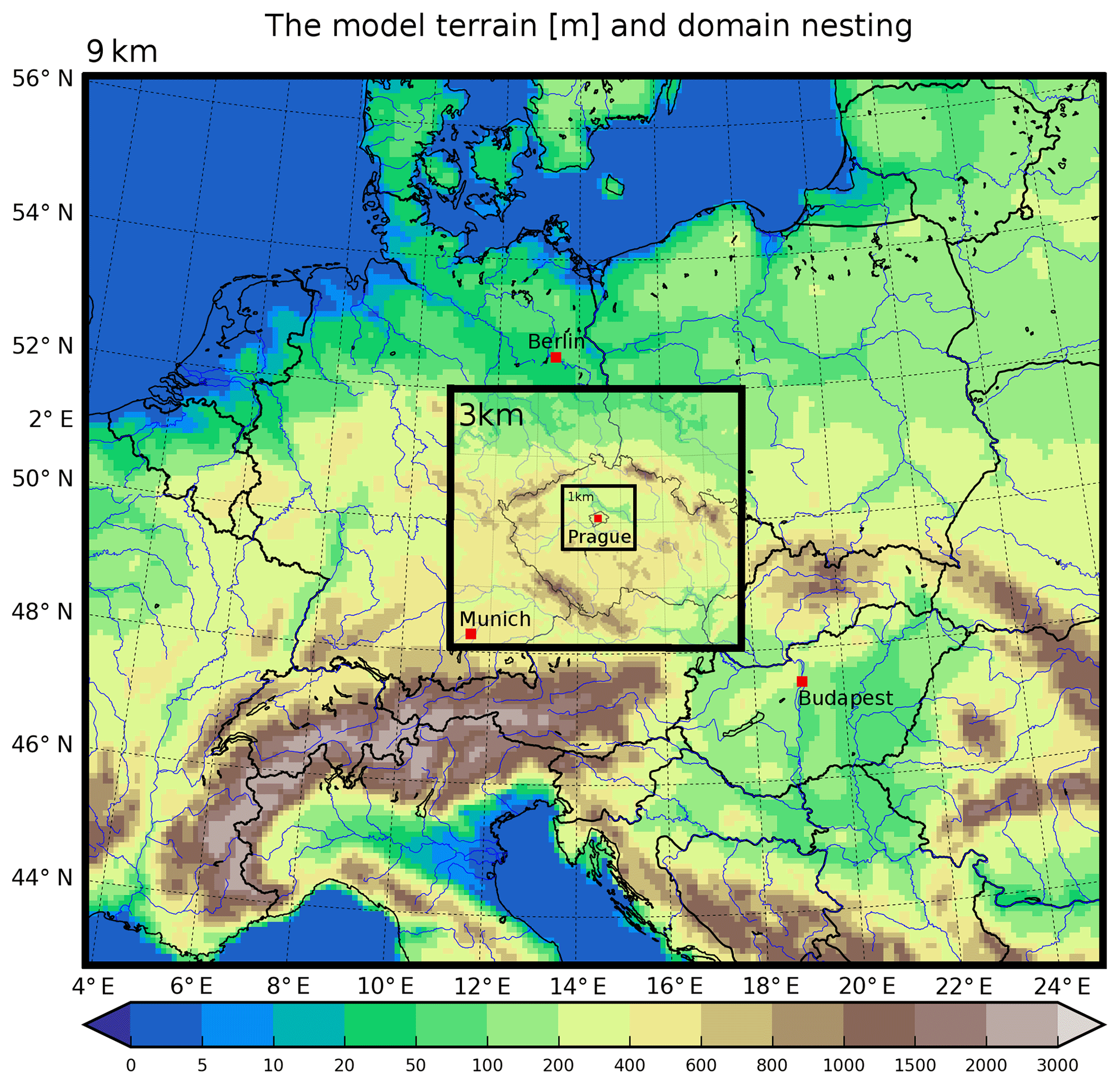
Figure 1 The resolved model terrain in meters, the nesting structure and the cities analyzed in the study (Prague, Berlin, Budapest, Munich).

Table 1 The list of model simulations performed. The first section contains the RCM simulations that cover the whole analyzed period with the information whether urban land surface was considered (2nd column). The second section lists the performed regional CTM experiments – here the second column provides information on the driving meteorological data (not needed in the case of WRF-Chem). Finally, the third section lists the RCM/CTM simulations conducted over the two selected air pollution episodes in 2015.

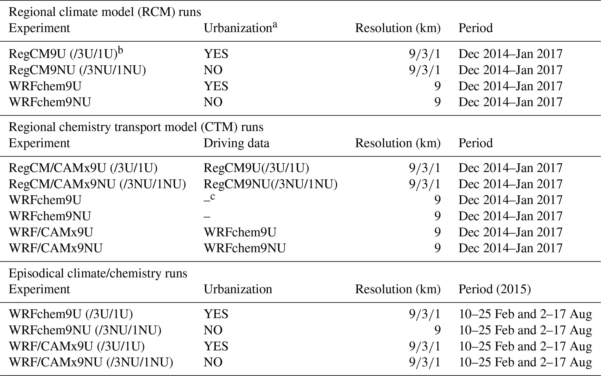
^a Information whether an urban land surface was considered. ^b Simulation performed in a nested way on 9, 3 and 1 km. ^c No driving meteorological data needed as chemistry is online coupled to the parent meteorological model.

The summary of all regional climate model (RCM) and chemistry transport model (CTM) simulations is given by Table 1. First, we performed experiments to analyze the urban canopy meteorological forcing over the 2-year period. These include RegCM experiments at all three resolutions with offline nesting and a 9 km WRF-Chem experiment. Apart from the default RCM runs where urban surfaces were taken into account and parameterized with the urban canopy models mentioned above, we performed in parallel experiments where urban surfaces were disregarded and replaced by a land-use type typical for the surroundings for the urban area (most of the time “crops”). Accordingly, the runs with “urban” surfaces considered are suffixed with “9U” (or “3U” or “1U”, for higher resolutions) and those not considering them (“nourban”) “9NU” (or “3NU” or “1NU”).

After the regional climate model runs, we performed the CTM runs using CAMx. For the WRF-Chem runs this means of course no additional experiments given its online coupled nature. CAMx runs performed using the RegCM meteorology that considers and parameterizes urban land surface are denoted as “RegCM/CAMx9U” (or 3U/1U for higher resolutions), while “RegCM/CAMx9NU” (or 3NU/1NU) denotes simulations driven by “nourban” meteorology. Additionally, the 9 km resolution WRF-Chem experiments serve as another CTM and finally, CAMx was driven also by the corresponding WRF-Chem meteorology denoted “WRF/CAMx9U” (or 9NU for the “nourban” case). Further, short-term climate-chemistry experiments were performed to demonstrate the UCMF impact on chemistry during extreme air pollution events. For these, WRF-Chem was run in a nested mode similar to RegCM and denoted as “WRFchem9U” (or 3U/1U, and for the “nourban” case: 9NU/3NU/1NU). Finally, these WRF-Chem runs served as a driver for CAMx to obtain a further set of short-term simulations: “WRF/CAMx9U” (or 3U/1U) and “WRF/CAMx9NU” (/3NU/1NU) for the “nourban” case. With this complex design of experiments, we could simultaneously investigate the long-term urban impact (according to Huszar et al., 2014, 2 years is a sufficiently long period for significant urban impacts in models) while giving the possibility of demonstrating the behavior of urban chemistry during high air pollution periods.

The outer 9 km domain simulations were forced by the ERA-Interim reanalysis (Simmons et al., 2010). The nested 3 and 1 km domains are forced by the corresponding parent domain using one-way nesting. Chemical boundary conditions for the outer domains were taken from the CAM-Chem global model data (Buchholz et al., 2019; Emmons et al., 2020). Land-use information adopted in model simulations was derived from the high-resolution (100 m) CORINE CLC 2012 land-cover data (https://land.copernicus.eu/pan-european/corine-land-cover, last access: 14 October 2020) and the United States Geological Survey (USGS) database, where CORINE was not available. An important difference between RegCM and WRF is that the former one, land use is represented as fractional, while in WRF, each grid box is attributed the dominant land use.

For European-scale emissions, the CAMS (Copernicus Atmosphere Monitoring Service) European anthropogenic emissions (CAMS-REG-APv1.1; Regional Atmospheric Pollutants; Granier et al., 2019) for the year 2015 were used. For the area of the Czech Republic, a high-resolution national Register of Emissions and Air Pollution Sources (REZZO) dataset issued by the Czech Hydrometeorological Institute (http://www.chmi.cz, last access: 14 October 2020) and the ATEM Traffic Emissions dataset provided by ATEM (Studio of ecological models; http://www.atem.cz, last access: 14 October 2020) were used. The listed emissions data provide annual emission totals of the main pollutants, namely NO_x, volatile organic compounds (VOC), SO₂, CO, PM_2.5 and PM_10. CAMS data are gridded data, while the Czech REZZO and ATEM datasets are defined as area, point and line (for road transportation) shapefiles of irregular shapes that correspond to counties and correspond to resolutions of from a few 100 m to 1–2 km depending on the geometry of the particular shape.

The original emission data from the listed emissions sources is preprocessed using the Flexible Universal Processor for Modeling Emissions (FUME) emission model (Benešová et al., 2018, http://fume-ep.org/, last access: 14 October 2020). FUME is intended primarily for the preparation of CTM ready emissions files. As such, FUME is responsible for preprocessing the raw input files and the spatial distribution, chemical speciation, and time disaggregation of input emissions. Emissions used are provided in 11 categories (SNAP – Selected Nomenclature for sources of Air Pollution) and category specific time disaggregation (van der Gon et al., 2011) and speciation factors (Passant, 2002) are applied to derive hourly speciated emissions for CAMx and WRF-Chem. Biogenic emissions of hydrocarbons (BVOC) for CAMx are calculated offline using the MEGANv2.1 (Model of Emissions of Gases and Aerosols from Nature) emissions model (Guenther et al., 2012) based on RegCM and WRF meteorology (except for the WRF-Chem experiments, where they were calculated online). Plant functional types, emission factors and leaf-area-index data were derived based on Sindelarova et al. (2014).

3 Results

3.1 Model validation

Here we provide a basic comparison of the most important modeled quantities to measured data (for both the meteorology and air quality).

3.1.1 Measurements used

For the validation of the modeled domain-scale meteorology, we used the European E-OBS (version 20.0e) $\mathrm{0.1}{}^{\circ }\times \mathrm{0.1}{}^{\circ }$ resolution gridded data (Cornes et al., 2018). For station-based validation over Prague, we used hourly series from two Prague stations (Praha-Libus/ALIBA and Praha-Suhdol/ASUCA) from the Czech Automatic Imission Monitoring network (AIM; http://portal.chmi.cz/aktualni-situace/stav-ovzdusi/prehled-stavu-ovzdusi, last access: 14 October 2020). These provide near-real-time measurements of the most important pollutants and also of basic meteorological variables, including temperature, humidity and wind speeds. For the planetary boundary layer height, ceilometer measurements conducted at Praha-Ruzyne (ALERA) station are used. These measurements use an enhanced gradient method to determine the PBL height (Vaisala, 2015).

Measurements of O₃ and NO₂ and PM_2.5 are taken from the AirBase: European Air Quality measurements (https://www.eea.europa.eu/data-and-maps/data/aqereporting-8, last access: 14 October 2020) dataset for all AirBase stations from Prague with a temporal coverage of the analyzed period. Only background stations (both urban and suburban) were considered. Traffic stations were omitted due to limited model resolution (1 km) incapable of resolving intense localized emissions.

3.1.2 Meteorology

Figure 2 presents the regional-scale domain-wide comparison of modeled and observed near-surface temperature and precipitation based on the E-OBS. RegCM shows overestimation of temperature, mostly during winter months by up to 2–3 ^∘C, especially over low lands. During JJA, the overestimation is slight higher; however, for the city of interest, Prague, the model lies within ±0.5 ^∘C. Over mountains, RegCM shows a systematic negative bias up to 3 ^∘C (up to 5 ^∘C for the Alps). In the case of WRF-Chem, temperature is rather underestimated by up to 1 ^∘C in both seasons and is in general in better agreement with observation compared to RegCM. The overestimation of urban temperatures is caused by the fact that E-OBS is interpolated and regridded from a relatively sparse network of stations unable to resolve local variation due to urban effects (Kyselý and Plavcová, 2010).

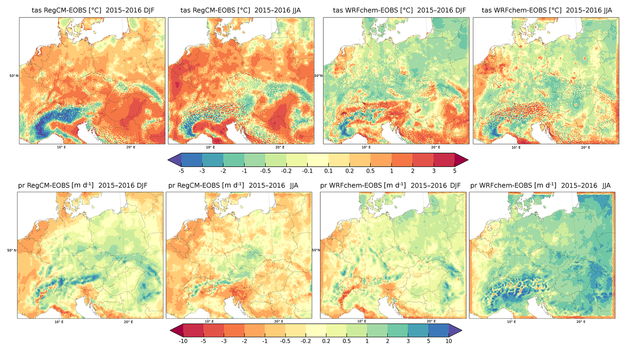
Figure 2 The difference between RegCM and WRF-Chem near-surface temperature (tas) in ^∘C (upper row) and the average daily precipitation (pr) in mm d⁻¹ (lower row) and E-OBS data for 2015–2016 DJF (1st and 3rd columns) and DJF (2nd and 4th columns) for the 9 km experiments in ^∘C. The boundary cells are affected strongly by the lateral boundary conditions being relaxed towards the domain interior causing different bias along the domain edges. These data should be ignored.

Precipitation is slightly overestimated in RegCM, especially in winter by up to 1 mm d⁻¹ on average. In JJA, the model–observation agreement is better, with biases within −1 to 1 mm d⁻¹; larger positive negative bias occurs over western and southeastern Europe. For WRF-Chem, winter is modeled with a fairly good agreement, with biases within −0.5 to 0.5 mm d⁻¹; however, the model overestimates precipitation during JJA by up to 3 mm d⁻¹. The boundary cells are affected strongly by the lateral boundary conditions being relaxed towards the domain interior causing different bias along the domain edges. These data should be ignored.

Figure 3 shows the model performance during the selected summer and winter periods for the most important meteorological quantities controlling air chemistry: near-surface temperature, 10 m wind speed and planetary boundary layer height. Regarding temperature during the summer episode, RegCM is able to capture daily maxima with much higher success than WRF-Chem, in which case the model bias reaches −5 ^∘C. For daily nighttime minima, however, RegCM shows a large positive bias (1–2 ^∘C), while WRF-Chem experiments are more in line with observations. For the winter period, the model–observation agreement is highly dependent on the day. While during the first part of the episode, characterized by strong inversion and low daily maxima, models tend to overestimate the diurnal temperature range, they agree better with measurements for days with higher temperatures, when low-level inversion clouds were dissipated. In general for the winter episode, the agreement is better for WRF-Chem experiments.

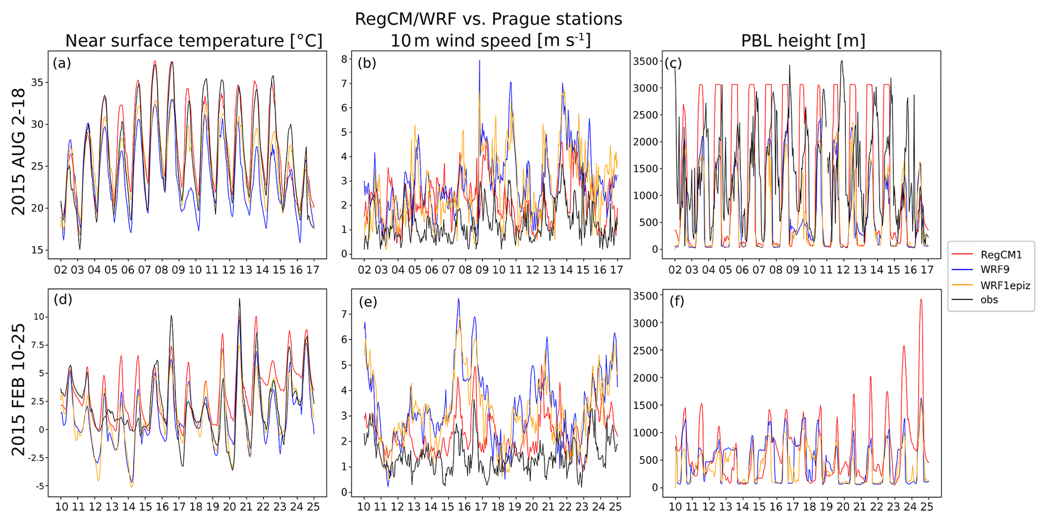
Figure 3 Comparison of modeled near-surface temperature (tas; a, d), 10 m wind speed (wind 10 m; b, e) and boundary layer height (PBLH; c, f) with station (average from two urban stations) data over Prague for the summer (a–c) and the winter period for RegCM simulations at 1 km resolution, for the 9 km WRF-Chem simulation and for the “episodical” WRF-Chem simulations at 1 km resolution (see Table 1).

Wind is systematically overpredicted by both models in both episodes by about a factor of 2 for RegCM, while WRF produces, in general, even larger wind speeds. The correlation with observation is much lower than in the case of temperature. One can also see that higher observed wind speeds are captured with smaller bias.

Observation of the boundary layer height (PBL) were deduced from ceilometer measurements, whose reliability depends on the meteorological conditions and have many shortcomings (Lee et al., 2019). Therefore, instead of point-by-point comparison, we focus on the model biases in terms of average values and maximum (minimum) daily boundary layer height. For the summer episode, RegCM produces usually higher PBL heights (except a few days). The PBL in this model is set to reach a maximum possible value (about 3000 m), which is evidently reached during almost all analyzed summer days. The average maximum PBL height in WRF-Chem experiments is around 2000 m, which means PBL height is slightly underestimated. During the winter episode characterized by low PBL height, its evolution is captured seemingly with a better accuracy for both models, while RegCM generates slightly larger PBL depths. A general behavior is that both models in both episodes tend to underestimate nighttime PBL heights connected to too stable stratification.

3.1.3 Air quality

Figure 4 presents a comparison of the modeled near-surface concentrations to AirBase data in terms of an annual cycle of monthly means, diurnal cycle and histogram (probability density function; PDF) of daily means.

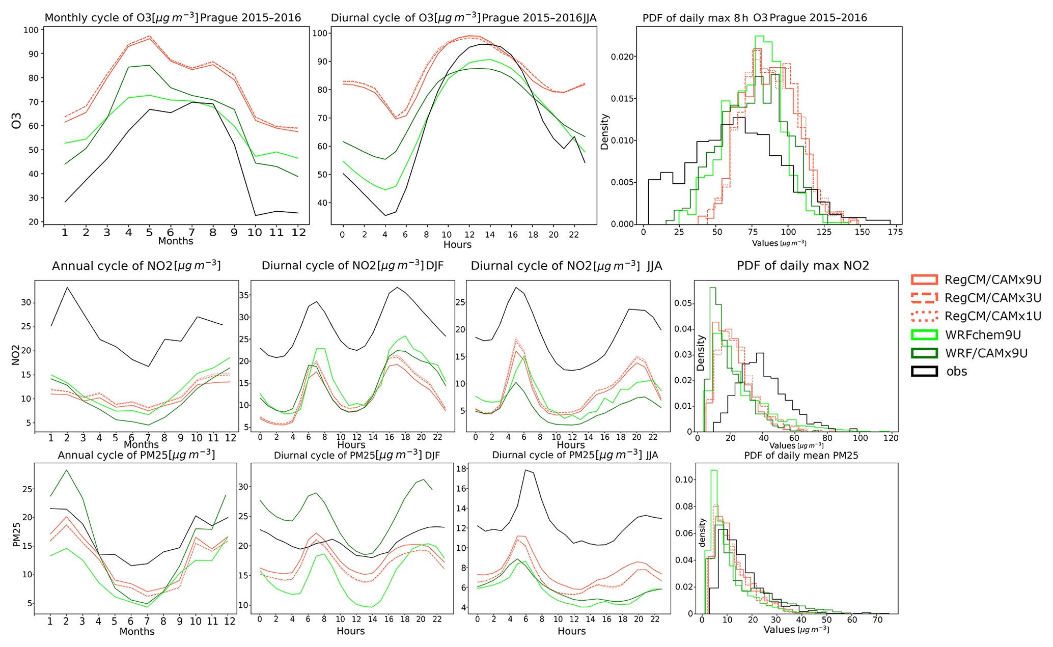
Figure 4 Comparison of modeled O₃ (up), NO₂ (middle) and PM_2.5 (bottom) near-surface concentrations with AirBase measurements over Prague. Three different statistics are evaluated for the 2015–2016 period: the average annual cycle, the average DJF and JJA diurnal cycle (for ozone only for JJA) and the histograms (probability density functions; PDFs) of the daily average values for the RegCM-driven CAMx simulations (red), for the 9 km WRF-Chem (light green) and WRF/CAMx (dark green) “urban” (U) experiments (see Table 1). Observational data in black. Units in µg m⁻³.

For ozone, there is a systematic overprediction of observed values for all models, while the RegCM-driven CAMx simulations exhibit the largest bias up to 20–30 µg m⁻³. Biases are smallest during summer months (almost zero for the WRF-Chem model), while large overestimation occurs during the colder part of the year. According to the diurnal cycle, daily ozone maxima are reasonably captured, with slight overestimation (underestimation) for RegCM (WRF) driven experiments, and the timing of maximum ozone is somewhat shifted (by about 1 h) in runs performed with CAMx. Large overestimation occurs during night, especially for RegCM-driven CAMx runs (up to 40 µg m⁻³), explaining the model bias during summer seen in the annual cycle. The histogram shows too that the distribution of modeled values has it maximum at larger values than the observed ones (around 80–90 µg m⁻³ compared to 60–70 µg m⁻³ measured). The low end of the measured distribution is poorly captured by all models.

NO₂ is underestimated by all models with a similar bias about 10–15 µg m⁻³ during all seasons (with slightly lower bias during summer). The systematic underestimation holds, according to the diurnal cycles, even for each hour. However, the model well correlates with measurements in terms of both the annual and diurnal cycles in both seasons. The underestimation is well implied from the histograms too, with the most probable model values lying around 10 µg m⁻³, while measured values have the most probable value, about 30–40 µg m⁻³.

Modeled PM_2.5 concentrations (on WRF-Chem output these are directly available, whereas in CAMx they have to be calculated as a sum of all primary and secondary aerosols) are usually underestimated, except the WRF-driven CAMx runs (WRF/CAMxU9) in winter. All model setups capture the annual cycle of PM_2.5 well, with summer values underestimated by about 5–10 µg m⁻³, especially in the WRF-driven experiments. The diurnal cycle of PM_2.5 in winter is characterized by two maxima resembling the emissions, which are present in the modeled values too, with a more pronounced amplitude. In general, the RegCM-driven CAMx (RegCM/CAMx) experiments are closer to measurements than the WRF ones.

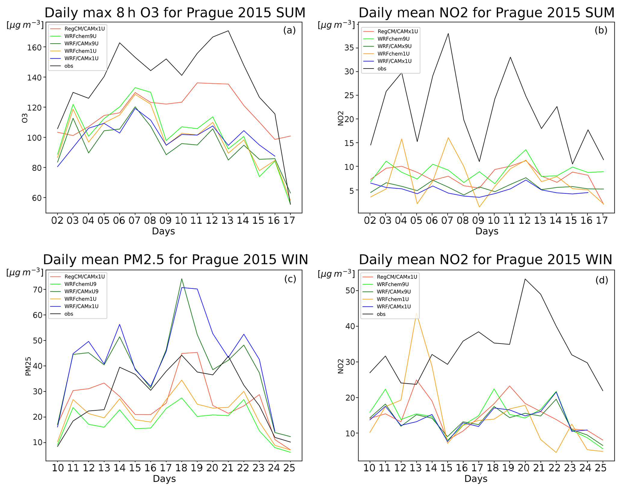
Figure 5 Comparison of modeled and observed maximum daily 8 h O₃ and daily mean PM_2.5 and NO₂ concentrations for the winter (a, b) and summer (c, d) periods for the 1 km RegCM-driven CAMx run (red), 1 km “episodical” WRF-Chem (orange) run, 1 km WRF-driven “episodical” CAMx run (blue), 9 km WRF-Chem run (light green) and 9 km WRF-driven CAMx run (dark green). All model results are from “urban” (U) experiments. Observational data in black. Units in µg m⁻³.

The model performance in terms of the daily maximum 8 h ozone, NO₂ and PM_2.5 near-surface concentrations and the corresponding observations during the two selected extreme air pollution episodes is presented on Fig. 5. Models underestimate the high ozone concentrations, with the best match for the RegCM-driven CAMx experiment. Although RegCM/CAMx, according to Fig. 4, slightly overestimates the daily maximum ozone on average, it is still unable to resolve extreme values as seen in the histogram. NO₂ is greatly underestimated during this episode, as expected from the general behavior seen on previous figure for all models. The models are poor in exhibiting this large negative systematic bias but also fail to capture the day-to-day variation. An exception is the 1 km WRF-Chem result, which could resolve the daily variation quite well. During the winter episode, PM_2.5 is underestimated by WRF-Chem and RegCM-driven CAMx runs, with the latter having smaller biases around −10 µg m⁻³. CAMx experiments driven by WRF meteorology tend to overestimate PM_2.5 during this episode. NO₂ is, as expected from the pervious figure (and similar to summer), underestimated (mainly its peak during 20–21 February), while high-resolution experiments (RegCM/CAMx and WRF-Chem) have a tendency to simulate peak values during the early days of the episode. This can be connected to underestimation of the PBL height seen in Fig. 3.

3.2 Impact on meteorology

Before looking at how extreme air pollution events respond to the introduction of urban surfaces (i.e., to the UCMF), we present how the meteorological conditions driving these air pollution cases change due to urban land surface. The most important three parameters will be analyzed that are a major part of the UCMF (Huszar et al., 2018a, b): the near-surface temperature (tas), the height of the boundary layer (PBLH) and the 10 m wind speed (wind10m). Apart from the changes in the mean values, we will also look at the changes at the tails of the probability distribution function (PDF) of these meteorological quantities. Indeed, extreme air pollution events are often related to high temperatures (high ozone episodes), low winds (stagnant conditions with limited dispersion from sources) and low boundary layer height (stable conditions with inversion layer(s) and very limited mixing).

3.2.1 Impact on average values

Figure 6 shows the average JJA and DJF urbanization-induced change in temperature, boundary layer height and 10 m wind speed for both RegCM and WRF-Chem 2015–2015 experiments as the difference between the “urban” (U) and corresponding “nourban” (NU) experiments for the area of Prague (with indicated administrative boundaries). To ease the comparison of the RegCM (performed at all three resolutions) performance with WRF-Chem (only 9 km), apart from the 1 km RegCM result, we also plot the result from the 9 km experiment.

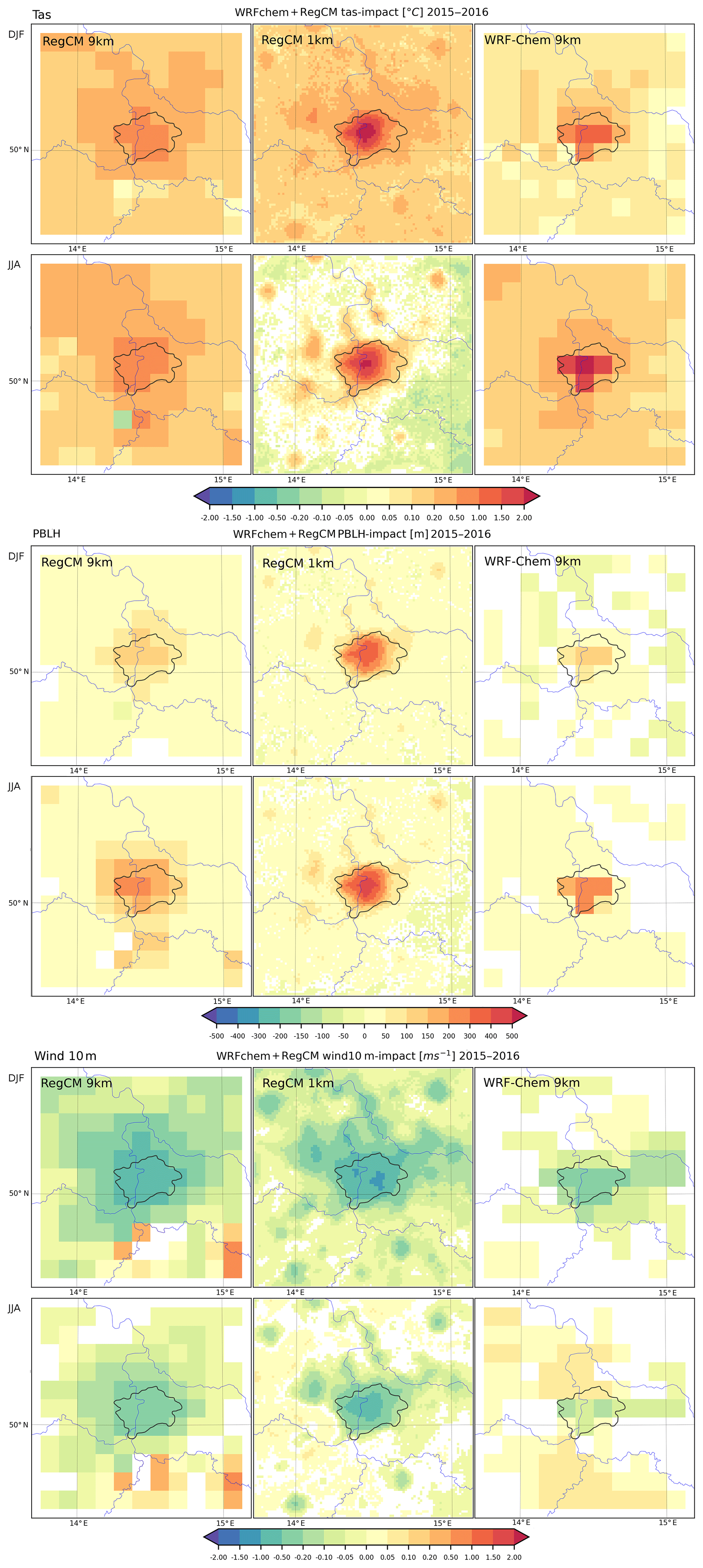
Figure 6 Components of the urban canopy meteorological forcing (UCMF) as the difference between “urban” (U) and “nourban” (NU) simulations for the 9 km RegCM, 1 km RegCM and 9 km WRF-Chem experiments for near-surface temperature (upper panel), boundary layer height (middle panel) and 10 m wind speed (bottom panel) for the area of Prague (with plotted administrative boundaries) as 2015–2016 winter (DJF) and summer (JJA) averages. White color represents statistically insignificant differences (98 % level; evaluated using a t-test).

Temperature is increased due to urban land surface by more than 1 ^∘C in summer for the 9 km RegCM run, while a much larger increase is resolved for the city center in the 1 km RegCM experiment (up to 3 ^∘C). WRF-Chem produces comparable increase around 2 ^∘C. For winter, the impact on temperature is weaker in RegCM compared to summer, except WRF-Chem, which produces again warming around 2 ^∘C. For the PBLH, the impact is larger during winter and most pronounced for the city center in the 1 km RegCM experiment (up to 300–400 m increase). In the 9 km experiments the increase is much smaller, reaching 150 and 300 m in summer and winter, respectively. Regarding the wind decrease, it is again most pronounced in the 1 km RegCM in the city center (around −1.5 m s⁻¹ change in summer). The winter decrease is in general lower, and the 9 km resolution runs produce lower wind decreases too (compared to the 1 km RegCM run), around −0.5 m s⁻¹. The figure clearly demonstrates the importance of resolution, with higher ones resolving the city center peaks of the impacts.

3.2.2 Impact on extreme values

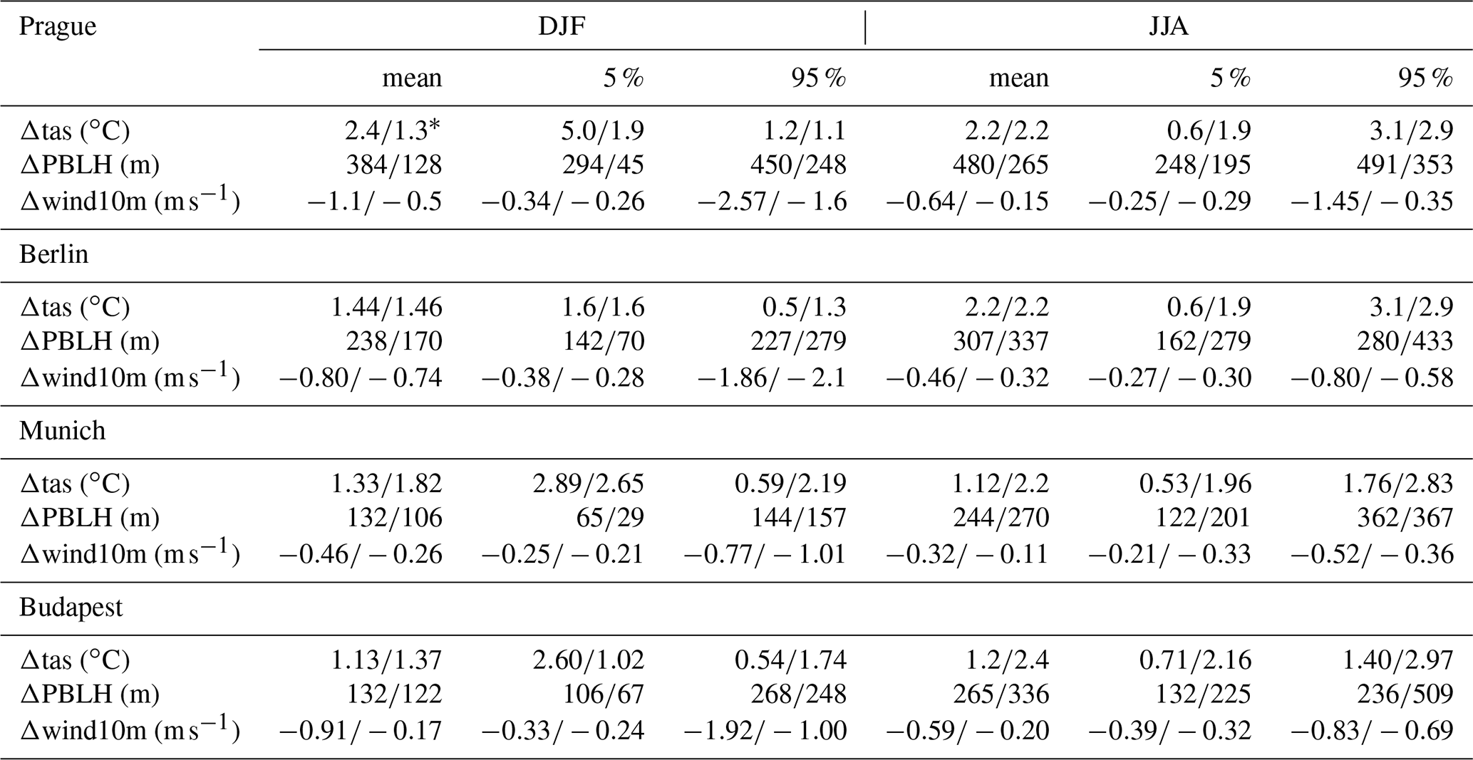
Apart from the change in the average values, we are also interested in examining how the above analyzed quantities change in their tails of the PDF. Results are summarized in Table 2 for four cities, Prague, Berlin, Munich and Budapest, and the 5th and 95th percentiles are analyzed (besides the mean values). The two numbers separated by a “slash” mean results for the RegCM and WRF-Chem simulations. Results are from the 9 km experiments except for Prague, whereas for the RegCM experiment we took results from the 1 km domain.

Table 2 Mean and 5 % and 95 % quantiles of the urban canopy impact for models RegCM and WRF on near-surface temperature (tas), the height of the boundary layer (PBLH) and 10 m wind speed (wind10m) averaged over DJF and JJA 2015–2016 for centers of four different cities. For Prague, values are taken from the 1 km simulations and 9 km for the rest.

^* RegCM vs. WRF(-Chem).

During winter, the 5th percentiles exhibit a larger increase compared to the change in means, although this depends on the model and city chosen. For Prague, the changes for the average values vs. 5th percentiles are 2.4 vs. 5.0 ^∘C in the 1 km RegCM run, while the differences for other cities and models are lower (around 1.5 vs. 2.0 ^∘C). The change in the 95th percentile is lower than the mean change for RegCM experiments and, for Berlin and Prague, also for the WRF-Chem ones. A more consistent picture is achieved for the JJA changes. In all models and for all chosen cities, the change in the 5th percentile value is lower than the change in the mean ones (0.5–2 vs. 1.2–2.4 ^∘C). On the other hand, the change in the 95th percentiles is larger than the change in the mean ones (1.5–3.0 ^∘C). In summary, in DJF low temperatures are increased more strongly due to urban land surface than the mean values, while in JJA, high values increase even more and low values are modified less due to the introduction of an urban land surface. This means that during summer, the PDF for temperature is wider after the rural-to-urban transformation.

For the PBLH, in DJF the 5th percentile change (around 50–250 m increase) is lower in every city and model than the change in the mean values (roughly 150–350 m increase). High increases are characteristic for the 95th percentile too (compared to the mean values), around 150–450 m. The general behavior of the PBLH and its change due to urbanization is similar in summer. While the change in the 5th percentile is somewhat smaller than the change in the mean values (120–250 vs. 240–480 m), the high end of the PDF responds with slightly higher increases (250–490 m).

In the case of wind-speed decrease at 10 m in DJF, the low end of the PDF responds less than the mean values (around −0.3 m s⁻¹ compared to −0.5 to −1 m s⁻¹). On the other hand, the decrease at the 95th percentile is much larger, around −0.7 to −2.5 m s⁻¹. Qualitatively a similar picture is seen for JJA, although the urbanization-induced changes are smaller. The change in the 5th percentile value is again around −0.3 m s⁻¹, i.e., less than the change in the mean ones (−0.3 to −0.5 m s⁻¹). On the other hand, the high end of the PDF corresponds to a stronger decrease (−0.3 to −1.5 m s⁻¹). In summary, higher wind speeds are prone to larger decreases due to the drag induced by the urban land surface.

3.3 Impact on the air quality

The above-presented meteorological changes (i.e., the UCMF) are expected to have implications for air pollutant concentrations, and here, we will also focus on the change in extreme concentrations; i.e., we will be interested in the behavior of the tails of the PDF. While from an AQ perspective, the high end of the PDF is of relevance, for completeness, we will also investigate the change in the low values. In particular, the 5th and 95th percentiles will be analyzed along with the change in the mean values. Spatial figures show the change for Prague (with indicated administrative boundaries) and its surroundings. Result are calculated as the difference between the corresponding “urban” (U) and “nourban” (NU) experiments.

3.3.1 Impact on ozone

In Fig. 7 the UCMF impact on JJA average and 95th percentile daily maximum 8 h O₃ (DMAX8HO3) is plotted for Prague. We are interested here in whether extreme values of DMAX8HO3 are impacted by the urban canopy meteorological forcing more than the mean values. As expected, the introduction of an urban land surface causes an increase in near-surface ozone concentrations. In the 1 km RegCM/CAMx experiment, the impact on mean is around 2–3 ppbv increase, while the 95th percentile is increased slightly more, by about 3–4 ppbv. The impact on mean values is similar for the 9 km RegCM/CAMx and, for WRF/CAMx experiments and these model setups, the increase at the high end of the PDF is also around 3–4 ppbv. For the WRF-Chem experiment, again, extreme values of DMAX8HO3 increase more (around 4–6 ppbv) compared to the change in mean values (3–4 ppbv).

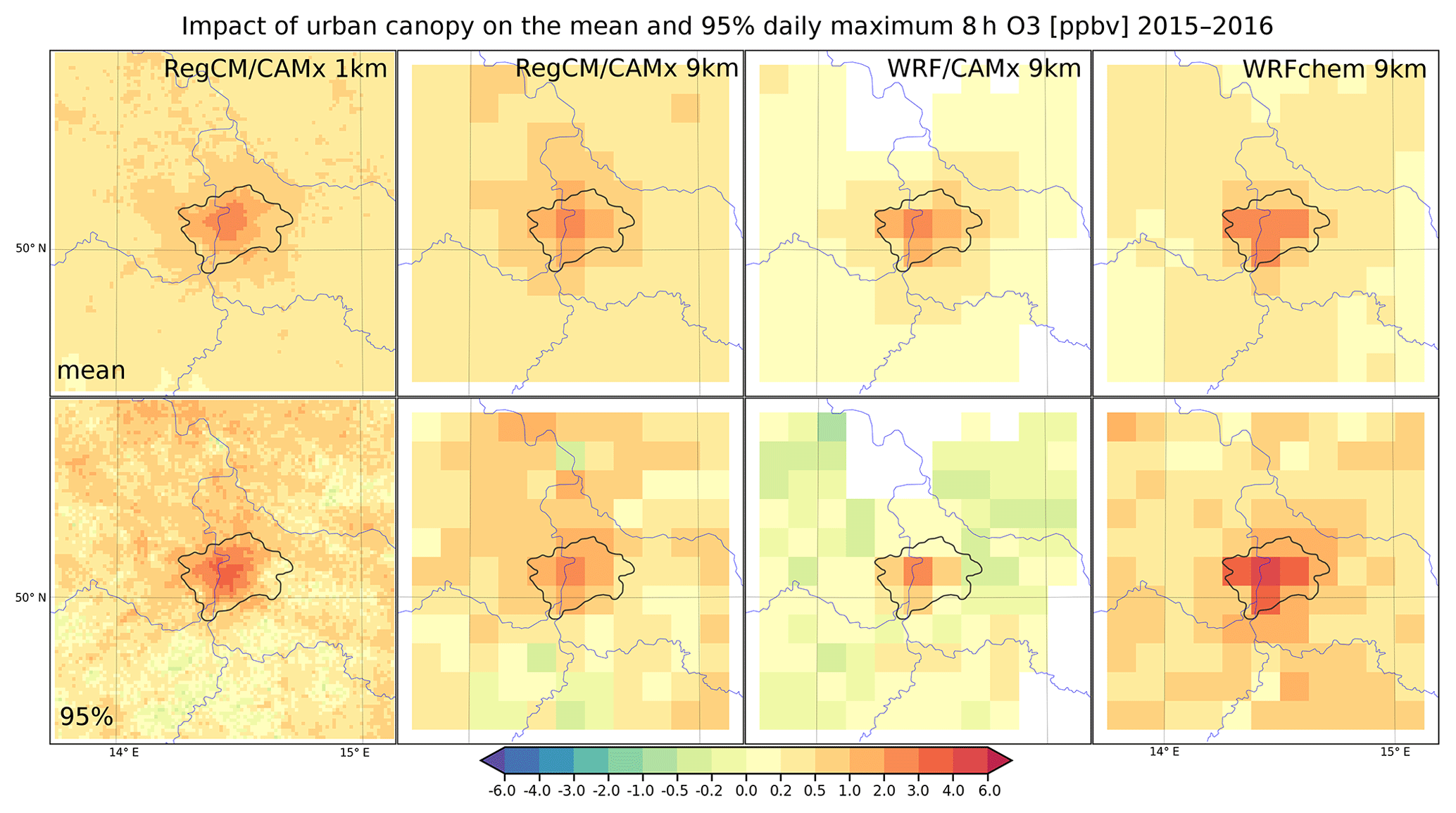
Figure 7 The UCMF impact on the 2015–2016 JJA mean (1st row) and the 95 % percentile (2nd row) O₃ in ppbv for the 1 km RegCM/CAMx, 9 km regCM/CAMx, 9 km WRF/CAMx and 9 km WRF-Chem experiments as the difference between the “urban” (U) and “nourban” (NU) simulations. White color represents statistically insignificant differences (98 % level; evaluated using a t-test).

To extend our analysis to a larger number of samples for obtaining more robust results, we summarized the urban-canopy-induced absolute change in ozone in the centers of four cities, Prague, Berlin, Munich and Budapest, and the results are presented in Table 3. Besides the mean and 95th percentile, we included for completeness also the JJA change in low values (5th percentile). Regarding the change in the lower end of the PDF, the picture is not clear, and both lower and higher changes with respect to the change in the mean values are encountered. For RegCM/CAMx, the change for the 5th percentile is usually lower, for WRF/CAMx, it is clearly higher, and for WRF-Chem, it is again rather lower than the corresponding change in the means. For the change in the high values (95th percentile), for RegCM/CAMx and WRF-Chem, there is an indication that the high end of the PDF responds to the UCMF, with a larger increase compared to the change in the mean values (2 to 4.5 vs. 2–3.5 ppbv); however, in WRF/CAMx, the changes in the 95th percentiles tend to be rather lower. In relative numbers (Table 4), the increase in the 5th percentiles is clearly higher compared to the relative change in mean values, and this holds consistently for each city and all model simulations. On the other hand, the relative increase in the 95th percentiles tends to be lower than the corresponding relative change in the mean values, and again, this holds for each city and every model.

Table 3 Mean, 5 % and 95 % quantiles of the urban canopy impact on JJA maximum daily 8 h ozone (DMAX8HO3) in ppbv for different city centers. Three numbers stand for the following experiments: RegCM/CAMx, WRF/CAMx, and WRF-Chem averaged over 2015–2016 for four different cities. For Prague and the RegCM/CAMx experiments, values are taken from the 1 km simulations and 9 km for the rest.

^* RegCM/CAMx, WRF/CAMx, WRF-Chem results.

Table 4 Same as Table 3 but in relative change with respect to the “nourban” (NU) case in %.

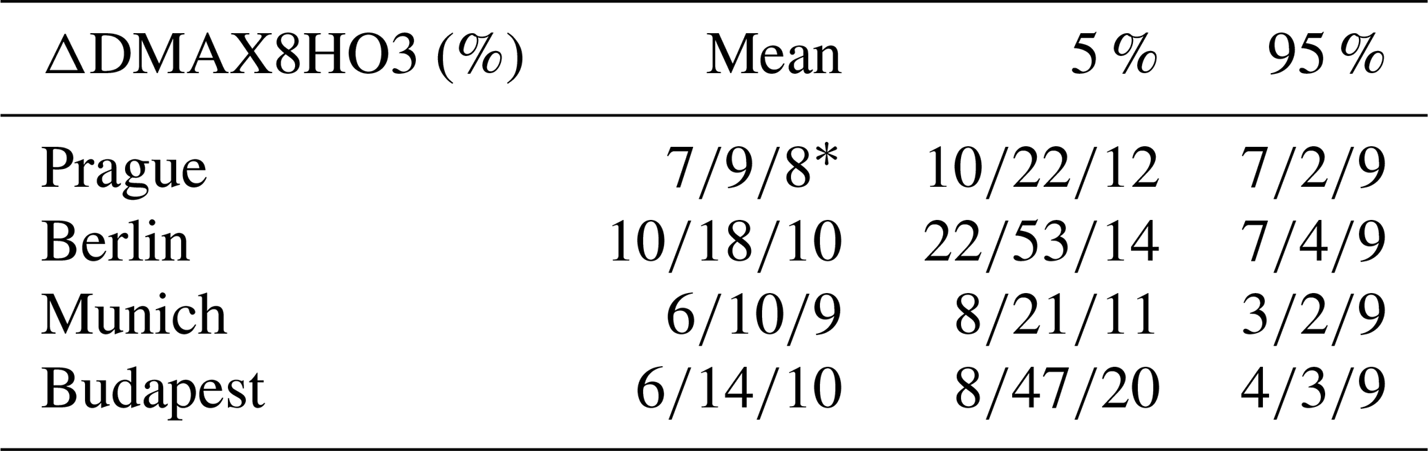
^* RegCM/CAMx, WRF/CAMx, WRF-Chem results.

3.3.2 Impact on NO₂

In Fig. 8 the UCMF impact on the DJF and JJA mean and 95th percentile daily mean NO₂ is plotted. The change in the average DJF concentrations is about −2 to −4 ppbv, being highest in the WRF-Chem experiment. Regarding the 95th percentile values, the change is evidently larger compared to the change in means. It is around −6 ppbv in both the 1 km RegCM/CAMx and WRF-Chem experiments, and somewhat lower, around −4 ppbv, in the rest of the simulations. In summary, results show an evidently larger decrease in extreme NO₂ values compared to the decrease in average values.

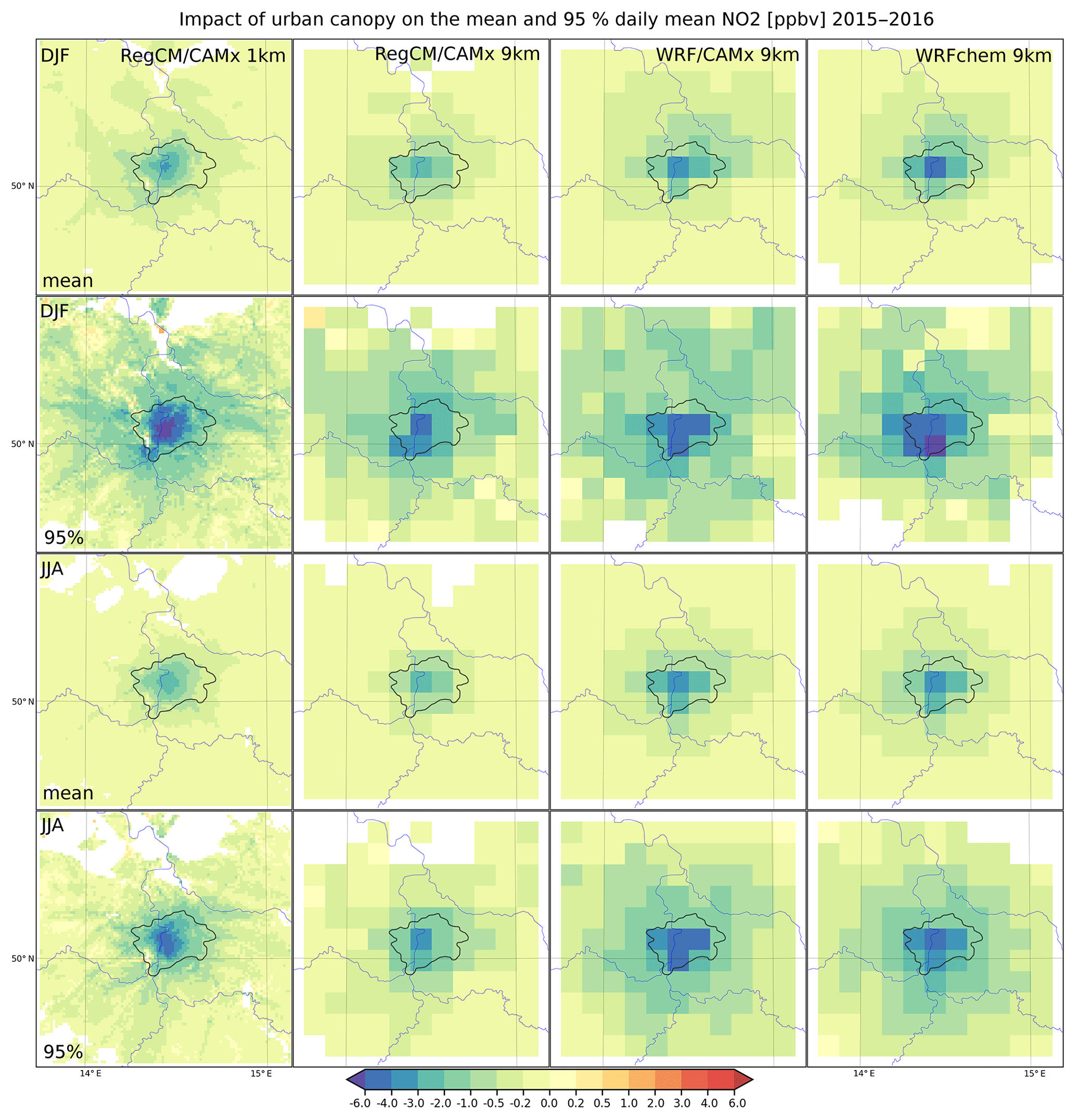
Figure 8 The UCMF impact on the 2015–2016 DJF and JJA mean (1st and 3rd rows) and the 95 % percentile (2nd and 4th row) NO₂ concentrations in ppbv for the 1 km RegCM/CAMx, 9 km regCM/CAMx, 9 km WRF/CAMx and 9 km WRF-Chem experiments as the difference between the “urban” (U) and “nourban” (NU) simulations. White color represents statistically insignificant differences (98 % level; evaluated using t-test).

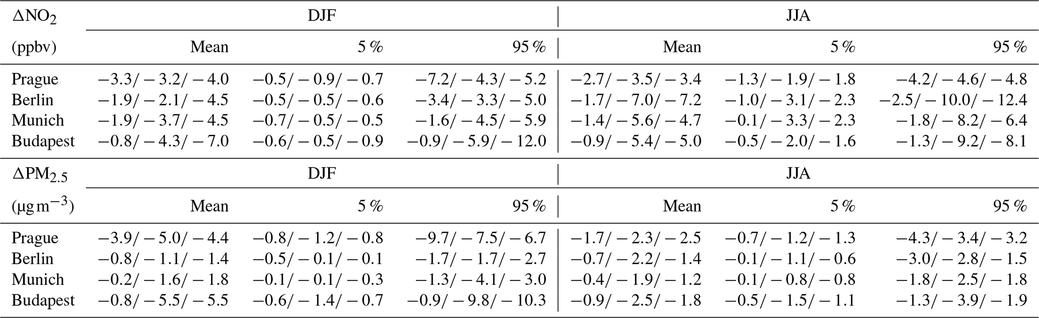
We extend our analysis again for other cities and to the changes in the low end of the PDFs too (see Table 5, upper part). Looking at winter 5th percentile values, it is evident for each city and model that these are prone to smaller reduction due to urban effects compared to mean values (around −0.5 to −1 ppbv change vs. −1 to −7 ppbv, depending on the city/model). The change in the 95th percentiles is on the other hand much larger (often 2 times) compared to the decrease in the mean values, in most of the cases ranging from −3 to −12 ppbv decrease (with the sole exception of Munich and the RegCM/CAMx run). The overall picture in JJA is qualitatively similar to the DJF case. While the decreases in mean values are between −1 and −7 ppbv, the decrease in the case of the 5th percentile is about −0.5 to −3 ppbv, and, on the other hand, the decreases in the 95th percentile values are much larger, lying between around −1.5 and −12 ppbv (largest in the WRF-driven experiments, usually above −5 ppbv).

As the urban canopy meteorological forcing (UCMF) induced NO₂ changes are caused primary by vertical turbulence transport (Huszar et al., 2020), the amount of removed material (i.e., the NO₂) is expected to be proportional to the absolute amount of that material. This could explain the larger change for the high end of the distribution. Whether this is true or other non-linear feedbacks play a role too, we also analyzed the relative change in the mean, 5th and 95th percentiles (as done for ozone too), and results are summarized in Table 6 (upper part). The relative changes in the 95th percentiles are shown only. For DJF, the relative change in the mean values is about −15 % to −20 %. For the 95th percentile change, the relative change is both larger and smaller depending on the city and model choice. Unlike in summer, the relative change in the 95th percentile values is evidently higher than the relative mean change, especially in the WRF-driven runs (WRF/CAMx and WRF-Chem), where it can exceed −50 % change compared to the −30 % to −40 % change for the mean values.

Table 5 Mean, 5 % and 95 % quantiles of the urban canopy impact on daily mean NO₂ and PM_2.5 in ppbv and µg m⁻³ for DJF and JJA. Three numbers stand for the following experiments: RegCM/CAMx, WRF/CAMx, and WRF-Chem averaged over 2015–2016 for the centers of four different cities. For Prague and the RegCM/CAMx experiments, values are taken from the 1 km simulations and 9 km for the rest.

3.3.3 Impact on PM_2.5

In Fig. 9, similarly to NO₂, the UCMF impact on the DJF and JJA average and 95th percentile daily mean PM_2.5 is plotted. In winter, the change in the mean values is around −2 to −4 µg m⁻³ in the RegCM-driven simulation up to −5 µg m⁻³ for WRF-driven ones for the center of Prague. The change in the 95th percentile is clearly larger: it reaches −6 µg m⁻³ in every simulation except the 9 km RegCM/CAMx experiment. In JJA, the UCMF-induced PM_2.5 changes are smaller. The change in mean values is around −2.0 µg m⁻³ (smaller only in the 9 km RegCM/CAMx experiment). Again, the change for the high end of the distribution is much larger and evident in each model. For the high-resolution RegCM/CAMx experiment, it reaches −4 µg m⁻³ but around −2 to −3 µg m⁻³ in other models. In summary, results show again evidently larger decreases in extreme PM_2.5 values compared to the decrease in mean ones.

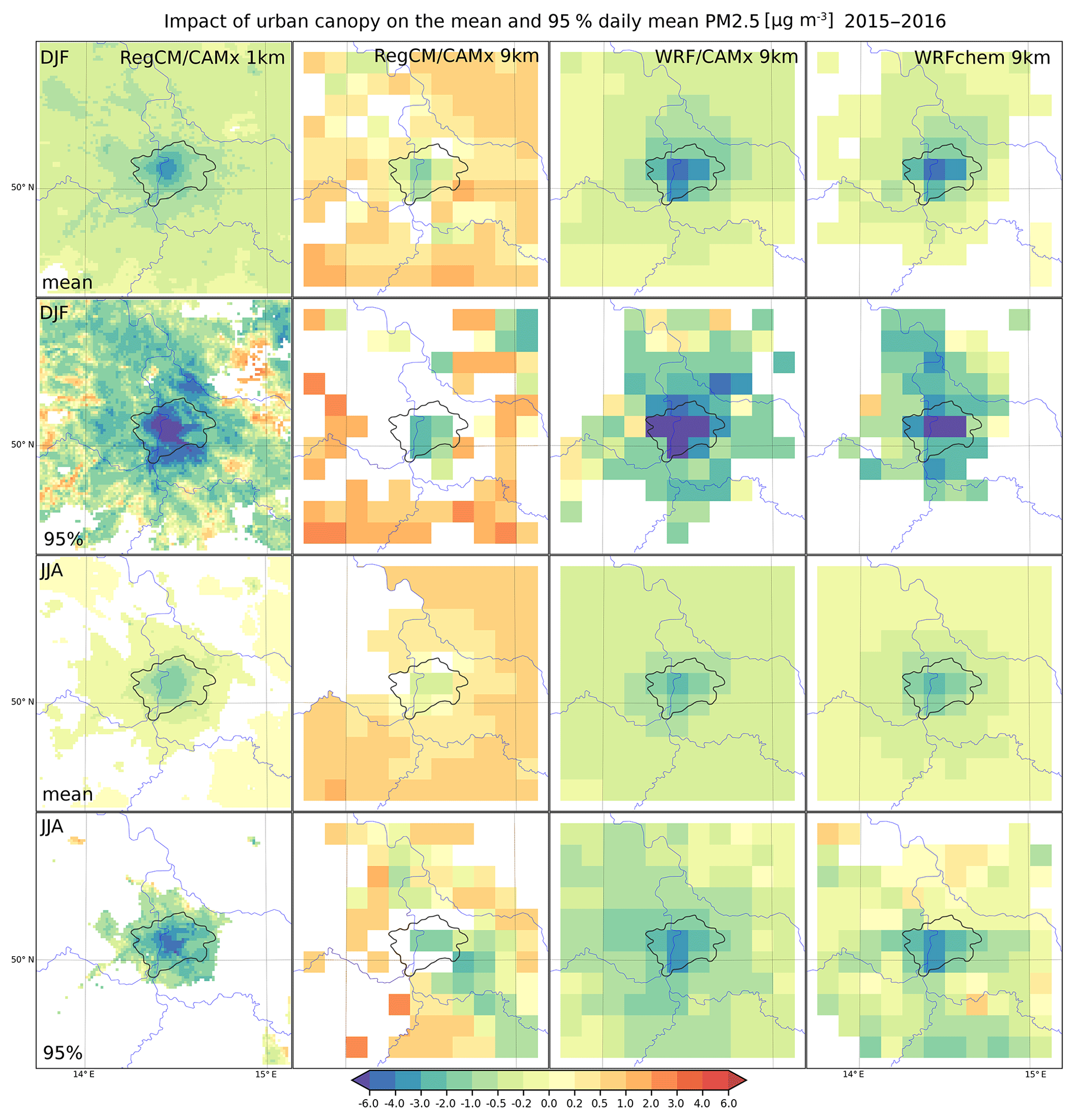
Figure 9 The UCMF impact on the 2015–2016 DJF and JJA mean (1st and 3rd rows) and the 95 % percentile (2nd and 4th row) PM_2.5 in µg m⁻³ for the 1 km RegCM/CAMx, 9 km RregCM/CAMx, 9 km WRF/CAMx and 9 km WRF-Chem experiments as the different between the “urban” (U) and “nourban” (NU) simulations. White color represents statistically insignificant differences (98 % level; evaluated using a t-test).

Table 6 Same as Table 5 but in relative change with respect to the “nourban” (NU) case in %.

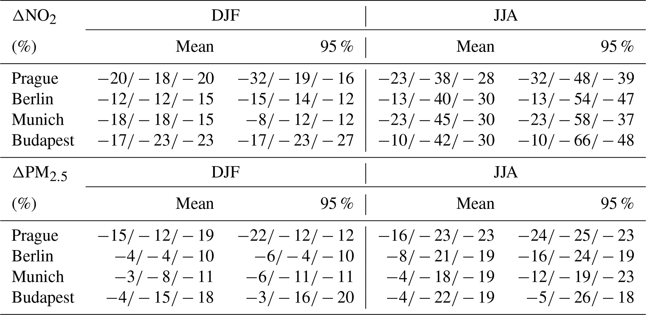
Extending our analysis again for other cities and also to the change in the low end of the PDF (Table 5), we can see in DJF that the 5th percentile changes are evidently lower than those of means, similarly to NO₂. The 95th percentile values (decreases) are however much larger, reaching −5 to −10 µg m⁻³ compared to changes in means (reaching −3 to −5 µg m⁻³). The JJA behavior is qualitatively similar to the DJF one: the changes in the 5th percentile values are smaller in an absolute sense compared to the change in means (up −0.1 to −1.5 vs. −0.5 to −2.5 µg m⁻³). Again, the 95th percentile changes are much larger compared to the change in means, reaching −4 µg m⁻³.

Looking at the relative changes in Table 6 (lower part) for DJF, there is an indication that the 95th percentile change is larger than the mean one in a relative sense, although models are not unified, and for some model experiments, the relative changes in 95th percentile vs. mean values are rather similar. In JJA, the relative change in the 95th percentiles is however clearly much higher than the corresponding change in the mean values, especially for the 1 km RegCM/CAMx experiment. In summary, the relative decrease in the 95th percentiles of PM_2.5 is similar to the relative mean change in winter; however, in summer, the relative change in the high-end values of PM_2.5 tends to be higher than the corresponding relative change in the mean ones.

3.3.4 Impact on concentrations during the episodes

In order to demonstrate how model concentrations respond to the introduction of urban surfaces (i.e., to UCMF) during episodes of extreme air pollution and whether the modeled changes in the high end of the distribution are in line with the model behavior during these episodes, we plotted the “urban” (U) and “nourban” (NU) evolution of the concentrations from different model experiments during these episodes; see Fig. 10. We also included the observed values in order to see how the model accuracy changes due to UCMF.

Looking at Fig. 10 upper panel with ozone, it is clear that urban effects, as expected, usually increase the simulated ozone. This increase is changing day by day and is different in each model but is around 5–10 µg m⁻³ on average, which is roughly 2.5–5 ppbv, i.e., very similar to the change in the 95 % percentiles seen in Table 3. The differences between the “U” and “NU” experiments are of course caused not only by the introduction of urbanized surfaces, but also by some higher-order effects (especially for secondary chemical species) that the urban canopy has on the physical properties of the air within and above this canopy; therefore, it is clear that during certain conditions, O₃ “nourban” values can be even higher compared to the “urban” values. For NO₂, the effect is more unified between models and confirms the results seen in Table 5: NO₂ concentrations due to the UCMF can be lower by up to 10 µg m⁻³ (roughly 5 ppbv), which is, again, very close to values for the 95 % percentile changes.

During the winter episode, PM_2.5 is clearly decreased by UCMF in every model and the decrease lies between 5 and 10 µg m⁻³ (largest in the WRF/CAMx experiments), which perfectly matches the interval seen for the 95 % percentile change in Table 5. The modeled “urban” and “nourban” NO₂ values during the winter episodes confirm the expected UCMF too: the “urban” values are lower by about 5–10 µg m⁻³, roughly 2.5–5 ppbv, compared to the “nourban” case. This is, again, in line with the values for the 95th percentile change.

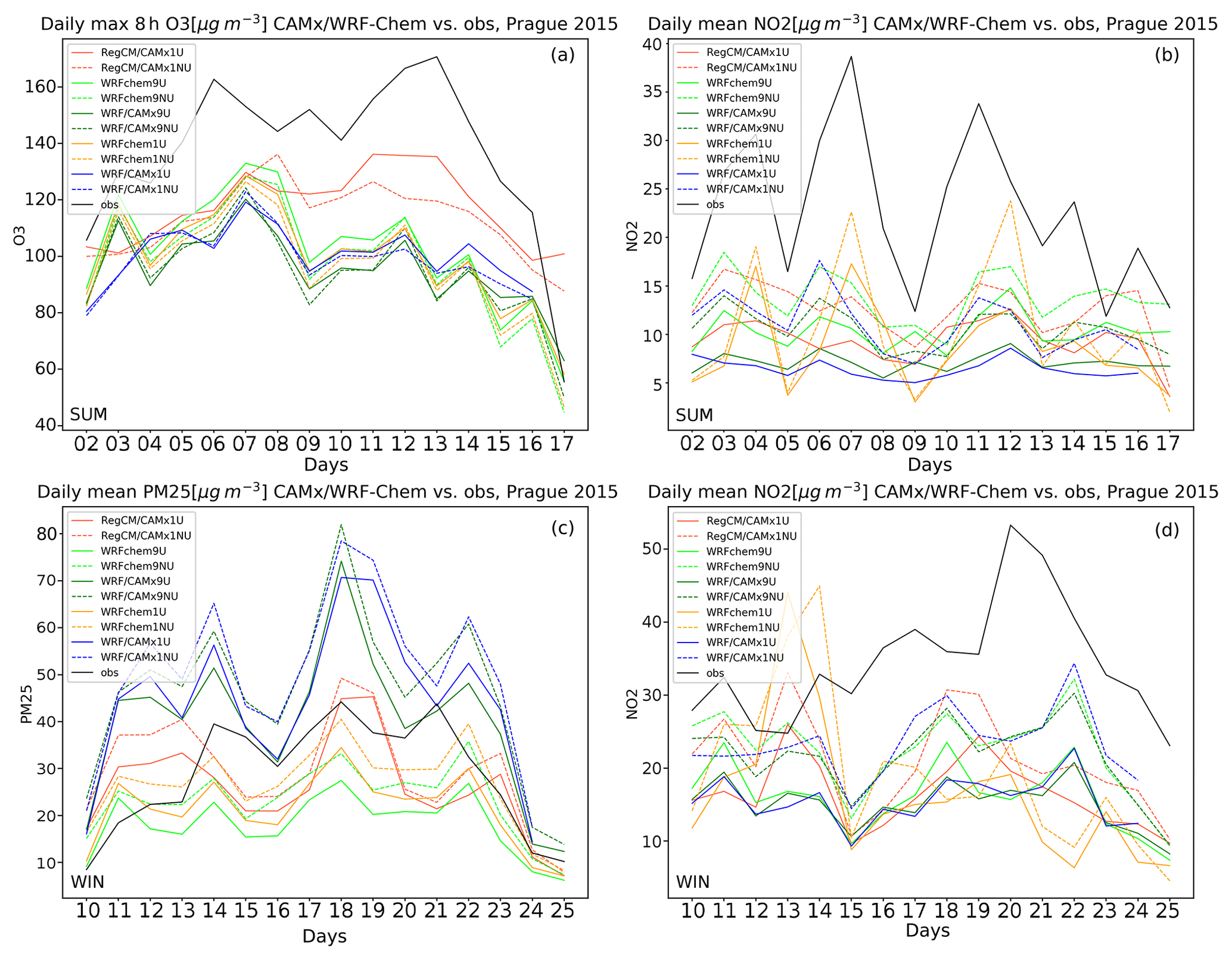
Figure 10 Comparison of the modeled and observed O₃ (a, c) and NO₂ (b, d) near-surface concentrations for the summer high ozone episode (a, b) and of the modeled and observed PM_2.5 (a, c) and NO₂ (b, d) near-surface concentrations for the winter high PM episode (c, d). Colors stand for different model simulations (Table 1): red stands for the 1 km RegCM/CAMx, green for the 9 km WRF-Chem, dark green for the 9 km WRF/CAMx and orange for the 1 km WRF-Chem and blue for the 1 km WRF/CAMx simulations. Black stands for observations. Solid line means “urban” (U), dashed “nourban” (NU) experiment. Units in µg m⁻³.

4 Discussion and conclusions

The study reveals some yet unanswered questions about the behavior of extreme air pollution concentration in reaction to the introduction of urbanized land surface. It adopted multiple regional climate model and chemistry transport model combinations and resolution to increase the robustness of the results and combined the analysis of both the long-term statistical behavior of air pollution as a response to UCMF, and its instantaneous response during particular extreme air pollution events.

4.1 Model validation

The general behavior of models in terms of simulating the average regional climate (within that we investigate the urban effects; Fig. 2) is that they perform reasonably with biases within the range of other similar studies (Berg et al., 2013; Huszar et al., 2014; Karlický et al., 2018; Huszar et al., 2020). In terms of RegCM, the large overestimation of precipitation seen in Huszar et al. (2020) is reduced by more than 50 % in this study, which can be attributed to the different moisture scheme used (WSM5 compared to the Nogherotto scheme). Winter temperatures have positive bias, connected probably to increased cloudiness (in connection with positive precipitation bias) and reduced thermal cooling. Giorgi et al. (2012), encountering similar biases, suggested that the heat removal from the surface towards higher levels is probably underestimated too. The seasonal temperature and precipitation biases are very similar to regional climate model studies Berg et al. (2013) and Fallmann et al. (2017), who used a similar resolution (7 km in their case) and the WSM5 microphysics too. In WRF, precipitation has a slightly higher positive bias than in RegCM experiments, and this can explain the negative temperature bias in summer (via enhanced cloudiness). In general, the six-class PLIN scheme counts with relatively high sedimentation velocities for graupel, which means stronger precipitation formation (via riming) (Hong et al., 2009), and this could contribute to the positive rain bias in WRF simulations. Gallues and Pfeifer (2008) showed that the PLIN scheme performs almost the best compared to other microphysics schemes in WRF; it has to be noted, however, that the observed biases in the model are a combined product of different parameterizations (including boundary layer, surface layer, land surface and other processes), and so far, according to the authors' knowledge, this combination has not yet been adopted in WRF studies.

During the two selected high air pollution episodes (Fig. 3), both models largely overpredict the 10 m wind speed, especially in winter. Giorgi et al. (2012) argued that the Holtslag scheme used in the RegCM setup overpredicts the vertical transport of momentum (and scalars too), causing stronger wind over the surface. In WRF-Chem the BouLac scheme was used that was found to better represent the PBL in regimes of higher static stability compared to non-local schemes; however, it still failed to predict the wind correctly, and it exhibits a similar overestimation to in, e.g., Tyagi et al. (2018). Similar overestimation of wind speed in WRF was reported also by Tucella et al. (2012). Another reason for wind overestimation can be related to the urban canopy models used (remember that observational data are from urban stations), and probably the urbanization-induced wind speed decrease is even larger than resolved by the models and their urban canopy schemes. PBL heights are simulated with acceptable accuracy with some overestimation in the RegCM model, which is probably connected to the overall overestimation of vertical turbulent transport of momentum in non-local schemes (like the Holtslag) (Giorgi et al., 2012) compared to the prognostic TKE-based schemes (Güttler et al., 2014; Wang et al., 2014). The average measured values are however within the model spread of PBLH values.

The comparison of modeled and observed pollutant concentrations reveals multiple model deficiencies (Figs. 4, 5). Ozone is strongly overestimated in monthly means given mainly by the nighttime positive bias (daytime values are captured reasonably). This behavior was encountered in previous regional climate-chemistry model studies with similar setups (Zanis et al., 2011; Karlický et al., 2017; Huszar et al., 2016a, 2018a, b, 2020) and is attributed to deficiencies in nighttime chemistry and also inaccurate vertical mixing in the nocturnal boundary layer (Zanis et al., 2011). During the selected summer episode, the 8 h ozone daily maxima are underestimated by all simulations, despite the fact that the maximum in the average diurnal cycle is captured more accurately. This indicates that the models are unable to correctly resolve the highest ozone values. WRF-Chem-simulated ozone values are systematically lower than CAMx values but show better correlation with the daily cycles, which is in line with the present finding of Flandorfer et al. (2020).

NO₂ is systematically underestimated in all models and suggests that emissions are too low or at least the NO+NO₂ speciation of NO_x emission is not correct. However, from the diurnal cycle in both summer and winter, it is clear that the correlation with observation is high, and this underlines the systematic character of the NO₂ average negative bias, which was similarly observed also in Huszar et al. (2016a) using very a similar model configuration, or also in Tucella et al. (2012) and Karlický et al. (2017), who both used WRF-Chem. The underestimation of NO₂ is clearly demonstrated also by the episode figures. Our results also show that high-resolution experiments are much more successful in capturing the day-to-day variation of pollutant concentrations, probably as a result of higher resolution of emissions and also a better representation of the terrain and therefore the meteorological conditions.

PM_2.5 is underestimated in our simulations, in both winter and summer (except one model setup, while overestimation occurs during winter). Huszar et al. (2016a) reported similar underestimations, which are attributable to underestimated nitrate aerosol and black/organic aerosol, as seen also in Schaap et al. (2004) and Myhre et al. (2006). Probably, emissions of the primary PM components are underestimated, similarly to their precursors (e.g., NO₂), pointing to the large role emissions play in the overall model biases (Aleksankina et al., 2019).

4.2 Impact on meteorology

The average impact on temperature (Fig. 6) has expected magnitude in our simulations compared to previous regional-scale studies conducted for European cities (Trusilova et al., 2008; Struzewska and Kaminski, 2012; Karlický et al., 2018; Huszar et al., 2020). There is an indication that higher model resolution leads to higher impact in city centers (seen for Prague); however, one must be careful with this conclusion, as, e.g., Huszar et al. (2020) reported a large impact also at relatively low resolutions and, even in our case, a similar magnitude of impact can be achieved with lower resolution applied in other models (e.g., WRF-Chem 9 km experiment vs. 1 km RegCM experiment). The changes in the height of the PBL are a little bit higher than values in our previous regional-scale study (Huszar et al., 2018a) or in Wang et al. (2007) and Zhu et al. (2017). They however used 3 km (and 9 km) as their highest resolution and, evidently, resolution plays role here, as in our case, the urban-canopy-induced PBL increase is much larger for the high-resolution inner domain compared to the coarse outer domains (where the increase is less by about 50 %) in both winter and summer. Summer PBL increase is higher, which is an expected consequence of enhanced contribution of a buoyant source of turbulence generation in urban areas (Fan et al., 2017) as a direct result of higher near-surface temperatures and thus reduced stability. In the case of the wind-speed changes, our results confirm the expected behavior that the winds are reduced due to the enhanced drag in urban areas. The reduction is greatest again for the high-resolution experiments, but the differences between low- and high-resolution results are rather small. Results are slightly smaller (around −1.5 m s⁻¹) compared to our previous study (up to 2 m s⁻¹ reduction) using a similar experimental configuration (Huszar et al., 2020) but are larger than in the coarse-resolution study of Huszar et al. (2018a). Wind decreases simulated for the central European region by Struzewska and Kaminski (2012) or for China by Zhu et al. (2017) are smaller, but this could again be the result of the coarser resolution they applied.

Our results show interesting features of the urbanization-induced modifications of extreme values of temperature, boundary layer height and wind speed (Table 2). During winter, the smallest temperatures are more affected than the average ones, which is probably caused by larger anthropogenic heat source during winter cold days, in contrast to warm winter days, when the additional heat input is smaller causing smaller temperature increase (Varentsov et al., 2018, and Karlický et al., 2018 showed that anthropogenic heat is an important contributor to the winter urban heat island). The situation in summer is opposite, and this reflects the drivers of the summer temperature increase in urban areas. Cold summer days with frequent cloudiness and limited sunshine are affected less due to the limited role of the radiation trapping. Hot summer days behave oppositely: during them the role of the short-wave radiative input from the Sun is much larger as well as the accumulation of heat due to multiple reflection and trapping in street canyons. Recently, Zhao et al. (2019) showed too that extreme temperature events (in terms of number of days with maximum temperature >25 ^∘C) are rapidly increasing in frequency with increasing urbanization.

The boundary layer height (PBLH) changes in the low and high ends of the probability distribution function show a more uniform picture: i.e., low values of PBLH change due to urbanization with a smaller magnitude than those corresponding to a thick PBL, in both studied seasons. This can be explained by the dependence of the urbanization-induced vertical turbulent diffusion (K_v) modifications on the absolute PBLH values, as shown by Huszar et al. (2020), who compared the magnitude of K_v for different turbulent parameterizations with the corresponding K_v modifications due to urban land surfaces. Indeed, during higher PBL characterized by stronger turbulent transport, an additional drag imposed by urban structures and heat source decreasing stability creates an increase in PBLH that is larger than the increase with weak turbulence. The dependence of the increase in boundary layer height and the absolute PBL is seen also from the diurnal cycles of K_v published in this study.

In the case of the wind-speed changes, a similar pattern is observed to that for the PBLH. Low wind speeds are modified by the introduction urban land surface less compared to high wind speed. Indeed, strong winds (95 % percentile values) are modified by almost a factor 2 more than average wind speeds. The reason for this is similar to PBLH changes: in the case of low winds, the additional drag due to urban land surface slows down the air motion to a lesser extent compared to high winds. This is seen also in the results of Huszar et al. (2020) showing that larger absolute wind speeds are associated with larger wind speed decrease. This is clearly visible even on the diurnal cycle of wind and its urban-induced changes (Huszar et al., 2018a): the largest absolute winds coincide with the large wind-speed decreases due to urban land surface. A similar finding was published in Zhu et al. (2017) too.

Relatively large differences in the average impact and that on extreme values (low/high percentiles) has been identified between cities and also between the two models implemented. While for Prague, RegCM results are obtained over 1 km, WRF-Chem was run on 9 km only which means that the urban core peak values are resolved in RegCM but not in WRF-Chem. For other cities that are represented at 9 km in both model results, the differences arise from rather the different representation of the urban land surface. Indeed, the dominant land use in WRF means that the urban fraction is strictly 100 % for a selected city, while in RegCM this is naturally less, resulting in stronger impact in WRF. This was previously encountered also in Karlický et al. (2018) and recently by Karlický et al. (2020). The differences between individual cities are easily explained by their different size corresponding to different fractional/dominant urban land cover (Berlin almost twice as large with twice the population of Munich or Budapest) but also to different background climates in which the UCMF acts (Zhao et al., 2014).

4.3 Impact on chemistry

The impact of the above discussed meteorological changes (what we call the urban canopy meteorological forcing – UCMF) on the average species concentration follows the expected patterns for each of the investigated species: ozone, NO₂ and PM_2.5 (Tables 3–6). In the case of ozone, the increases are a result of competing effects of increased eddy removal of NO_x and hence reduced titration leading to ozone increases, while on the other hand, smaller winds and higher temperature reduce ozone advection towards cities and enhance the dry deposition (Huszar et al., 2018a). In the case of NO_x and PM_2.5, the most important contributors are the reduced winds leading to concentration increases vs. increased vertical eddy transport reducing near-surface concentrations with later overweighting of the wind effects (Huszar et al., 2018b, 2020). For secondary aerosols, the temperature increases in urban areas also contribute to reduced concentrations. Our results here are in line with a number of previous studies: e.g., Civerolo et al. (2007) modeled the maximum 8 h ozone increases up to 6 ppbv, same as in our study. Jiang et al. (2008) and Xie et al. (2016a) found increases in O₃ due to rapid urbanization and the associated anthropogenic heat around 3–4 ppbv, again close to our finding. Huszar et al. (2020) calculated ozone increase due to enhanced urbanization-induced turbulence up to 3–4 ppbv; however, they concerned the change in seasonal average ozone (with similar changes to Jacobson et al., 2015), which can be in general different from the change in the maximum 8 h ozone. The resolution plays rather a minor role in the modeled magnitude of ozone changes, as seen in this study or noted by Markakis et al. (2015) too, who simulated the regional-scale air quality of Paris. Around a 3 %–4 % increase in surface ozone is calculated by Wang et al. (2009) due to urbanization, similar to our relative mean 8 h ozone changes (these are not directly comparable but give at least some first estimate of the differences between these studies). Martilli et al. (2003) simulated peak ozone changes around 10–20 ppbv, which are again not comparable to our 8 h averages but suggest that the urban impact on extreme ozone values can reach very high numbers.

Our results showed that the peak (95th percentile) 8 h ozone values increased due to urban meteorological effects by a little bit more than the mean values of this quantity, but this increase is not detectable in all model experiments and is seen mainly for the high-resolution ones (and also for the WRF-Chem case; Fig. 7). Jiang et al. (2008) also looked at changes in the frequency distribution of maximum 8 h ozone and, according to their results, the high end of the distribution changes by a similar magnitude to the median value, although it has to be noted that the changes due to climate change were included too. To conclude, simulations show that urbanization contributes to extreme ozone concentrations, but this contribution is rather similar to the contribution to the mean values or at least depend on the model setup.

With regard to changes in NO₂, there is a clear decrease ranging from −2 to −6 ppbv depending on the model and resolution applied and being slightly higher for winter. The decrease is explained by increased vertical turbulent transport (Huszar et al., 2018a; Kim et al., 2015; Xie et al., 2016a) and the numbers are close to previous studies (e.g., Sarrat et al., 2006; Struzewska and Kaminski, 2012). Our simulations showed a very important feature, i.e., that days with extreme (95th percentile) NO₂ pollution are much more affected (almost by a factor of 2) than the average days (i.e., those with average values) in both cold and warm seasons (Fig. 8). This is in line with previous studies that looked at selected air pollution episodes with high NO_x levels. For example, Sarrat et al. (2006) simulated an anticyclonic situation with weak winds and significant solar radiation when high values of ozone and NO_x occurred over Paris. Indeed, their results for NO₂ decreases are very large (more than −50 ppbv), supporting our findings that extreme air pollution events (for oxides of nitrogen in this case) are more influenced by the urbanization-induced meteorological changes than long-term average pollution.

The simulated PM_2.5 response to UCMF follows the know pattern too, which means mostly decreases that are larger in winter than in summer (about −4 and −2 µg m⁻³ decreases for the average seasonal concentrations, respectively). The intermodel differences and those arising from different resolutions seem to play a rather minor role, with stronger impacts simulated with higher-resolution RegCM experiments and with the WRF runs. The impact is stronger than in Huszar et al. (2018b), where the competition between wind-induced increases and turbulence-induced decreases resulted less in favor of turbulence and gave wind players a stronger role, similarly to Huszar et al. (2020). On the other hand, a similar decrease was modeled using WRF in Kim et al. (2015) for Paris, as in our study. Li et al. (2019b) found that the decrease in PM_2.5 due to urbanization is mainly detectable during nighttime and attributable to increased ventilation and gas-particle phase partitioning effects favoring the gas phase. In our simulations, there is a substantial difference between the change in the average values and those corresponding to the 95th percentile values – these latter are almost 2 times higher, especially for high resolutions (Fig. 9). This conclusion is similar to the NO₂ case. Both results suggest that the meteorological modification triggered by urban canopy alone has a strong cleansing effect on NO_x and PM_2.5 pollution and thus can counteract the primary sources of pollution, which are the urban emissions. This is especially true for extreme air pollution events (Fig. 10).

Similarly to inter-city and inter-model differences in the meteorological impacts, the impact on chemical concentrations exhibits a relatively large spread. This is of course explainable partially by the meteorological differences that drive chemistry but also due to differences between emissions which are proportional roughly to city size. Indeed, the impact for Munich, the smallest city analyzed, is often the smallest. On the other hand, the impact for Prague over 1 km in RegCM is the highest, pointing out the importance of high-resolution treatment, which is able to resolve urban core values (Markakis et al., 2015).

It has to be noted that in the case of UCMF-induced decreases in PM_2.5 and NO₂, one can expect that the change is somewhat proportional to the absolute values. Thus it will be higher for higher absolute values and, hence, the peak (e.g., 95th percentile) values will be more affected. To address this issue in more detail, we looked also at the relative changes in these pollutants, and they showed for summer and mainly for NO₂ that the relative modifications are larger for the peak (95th percentile) values. For winter, however, the relative changes rather follow the above expectation. To conclude, urbanization contributes to NO₂ and PM_2.5 extreme pollution negatively by decreasing their concentrations, which is shown to be stronger than the decrease encountered for the average values representing average air pollution conditions.

In summary, our paper focused on the investigation of whether extreme air pollution concentrations are affected by the urbanization-induced meteorological modifications with the same magnitude as the average values or whether the influence is much larger (smaller). We found that for maximum 8 h ozone, the influence is comparable for average and peak values – unlike for extreme NO₂ and PM_2.5, which responded to these meteorological modifications much more pronounced compared to the change in average values. This indeed underlines the important role that urbanization and the accompanying meteorological influences play during adverse air pollution episodes and has to be taken into account in policy making for which extreme air pollution in urban areas is much more relevant than average conditions. One has to, however, remember that our paper shows only a partial link in the rather complicated “urban/meteorology/air-quality” system. While urban canopies act differently to rural areas in the way the surface “communicates” with the overlying air and, as shown above (and in many previous studies), have a very specific impact on air chemistry and the three-dimensional transport of pollutants, it has to be kept in mind that extreme air pollution in urban areas is a combination of other components of the “urban/meteorology/air-quality” system: emissions play of course an important role, but large-scale meteorological features (over synoptic scales) can largely contribute too (Sun et al., 2019). Finally, our results also pointed out the important role high resolution plays. As such, peak urban impacts are much more resolved. In order to gain a more robust picture including many cities, such high resolutions should be applied to not only one city (with the rest analyzed in lower resolution), but also simultaneously for many others. Future modeling of the “urban/meteorology/air-quality” should go in this direction.