Craig–Gordon model validation using stable isotope ratios in water vapor over the Southern Ocean

The stable oxygen and hydrogen isotopic composition of water vapor over a water body is governed by the isotopic composition of surface water and ambient vapor, exchange and mixing processes at the water–air interface, and the local meteorological conditions. These parameters form inputs to the Craig–Gordon models, used for predicting the isotopic composition of vapor produced from the surface water due to the evaporation process. In this study we present water vapor, surface water isotope ratios and meteorological parameters across latitudinal transects in the Southern Ocean (27.38–69.34 and 21.98–66.8^∘ S) during two austral summers. The performance of Traditional Craig–Gordon (TCG) (Craig and Gordon, 1965) and the Unified Craig–Gordon (UCG) (Gonfiantini et al., 2018) models is evaluated to predict the isotopic composition of evaporated water vapor flux in the diverse oceanic settings. The models are run for the molecular diffusivity ratios suggested by Merlivat (1978), Cappa et al. (2003) and Pfahl and Wernli (2009), referred to as MJ, CD and PW, respectively, and different turbulent indices (x), i.e., fractional contribution of molecular vs. turbulent diffusion. It is found that the ${\mathrm{UCG}}_{x=\mathrm{0.8}}^{\mathrm{MJ}}$, ${\mathrm{UCG}}_{x=\mathrm{0.6}}^{\mathrm{CD}}$, ${\mathrm{TCG}}_{x=\mathrm{0.6}}^{\mathrm{MJ}}$ and ${\mathrm{TCG}}_{x=\mathrm{0.7}}^{\mathrm{CD}}$ models predicted the isotopic composition that best matches with the observations. The relative contribution from locally generated and advected moisture is calculated at the water vapor sampling points, along the latitudinal transects, assigning the representative end-member isotopic compositions, and by solving the two-component mixing model. The results suggest a varying contribution of the advected westerly component, with an increasing trend up to 65^∘ S. Beyond 65^∘ S, the proportion of Antarctic moisture was found to be prominent and increasing linearly towards the coast.

1 Introduction

The knowledge of factors governing the evaporation of water from the oceans is an essential part of our understanding of the hydrological cycle. The oceans regulate the climate of the earth through heat and moisture transport (Chahine, 1992). Nearly ∼97 % of the water of earth is in the oceans and saline, while the residual ∼3 % is fresh water stored in groundwater, glaciers and lakes or flows as rivers and streams (Korzoun et al., 1978). Evaporation of ocean water generates vapor and forms the initial reservoir for circulation in the hydrological cycle. A fraction of this vapor, only ∼10 % of it, is transported inland to generate precipitation, while rest of the moisture precipitates over the ocean during its transit (Oki and Kanae, 2006; Shiklomanov, 1998). Measurements of the isotope composition of water in the various reservoirs of the hydrological cycle operating over the oceans is useful to infer information about the origin of water masses and to understand the formation mechanisms, transport pathways and finally the precipitation processes (Craig, 1961; Dansgaard, 1964; Yoshimura, 2015; Gat, 1996; Araguás-Araguás et al., 2000; Noone and Sturm, 2010; Gat et al., 2003; Benetti et al., 2014; Galewsky et al., 2016). A comparatively large volume of data exists over land to understand the terrestrial hydrological cycle, through the Global Network of Isotopes in Precipitation (GNIP) initiative of the International Atomic Energy Agency (IAEA). However, only a handful records on the spatial and temporal variability in precipitation and vapor isotopic composition over the oceans are available for any assessment (e.g., Gat et al., 2003; Uemura et al., 2008; Benetti et al., 2015, 2017b, a; Rahul et al., 2018; Prasanna et al., 2018; Bonne et al., 2019). Hence, further effort is needed to enhance the spatial and temporal sampling coverage over the oceans.

The isotopic composition of vapor on top of a water body is governed by the following factors: (i) thermodynamic equilibrium process for phase transformation at a particular temperature, (ii) kinetic or nonequilibrium processes where role of relative humidity and wind is significant, and (iii) large-scale transport and mixing – due to the movement of air parcels laterally and vertically. Craig and Gordon (1965) initially proposed a two-layer model to simulate the isotopic composition of evaporation flux (referred to as the Traditional Craig–Gordon model). Recently, Gonfiantini et al. (2018) put forward a modified version referred to as the Unified Craig–Gordon Model. Both of these models incorporate the equilibrium and kinetic processes to simulate the isotopic composition of evaporated moisture. However, in order to get a realistic picture of the hydrological cycle over the ocean, the horizontal transport/advective mixing is important and should be incorporated. In this paper we present stable isotope ratios in water vapor and ocean surface water from different locations covering varied oceanic settings – i.e., tropical, subtropical and polar latitudes, with a large range in the sea surface temperature, relative humidity and wind speed. While the role of temperature-dependent equilibrium fractionation is well understood, the role of kinetic processes is under debate and requires further scrutiny. The performance of these Craig–Gordon evaporation models to simulate the isotopic composition of evaporation flux is evaluated along the sampling transect for different molecular diffusivity ratios and different fractions of molecular vs. turbulent diffusion in the framework of the global closure assumption. The evaporation flux is calculated by the Craig–Gordon models assuming the “global closure” – i.e., the isotopic composition of atmospheric vapor is equal to the isotopic composition of evaporation. The models and the conditions that best match with the observations are identified, which are then used to calculate the local evaporation flux. This is done in the context of estimating the contribution of advected vs. in situ-derived vapor along the sampling transect assuming a complete mixing of the advected and the locally generated vapor in the sampled water vapor in our study.

2 Methods

2.1 Sampling, isotopic analysis and meteorological parameters

The samples (water vapor and surface water) for this study were collected along the stretch from Mauritius to Prydz Bay (24–69^∘ S, 57–76^∘ E) during two successive austral summers – January 2017 (SOE-IX) and December 2017 to January 2018 (SOE-X) – onboard the ocean research vessel SA Agulhas. The water vapor sampling inlet was set at ∼ 15 m above the sea level. An aggregate of 71 water vapor samples were collected during the two expeditions. Figure 1 shows the water vapor sampling locations. Alongside water vapor, 49 surface water samples were also collected. The details about the sampling procedures for collection of water vapor and surface water samples are given in the Supplement. All these were subjected to isotopic analysis using a Finnigan GasBench peripheral connected to an isotope ratio mass spectrometer (Thermo Scientific MAT 253) (details are provided in the Supplement). The isotope ratios are expressed in per mill (‰) using the standard δ notation relative to Vienna Standard Mean Ocean Water (VSMOW).

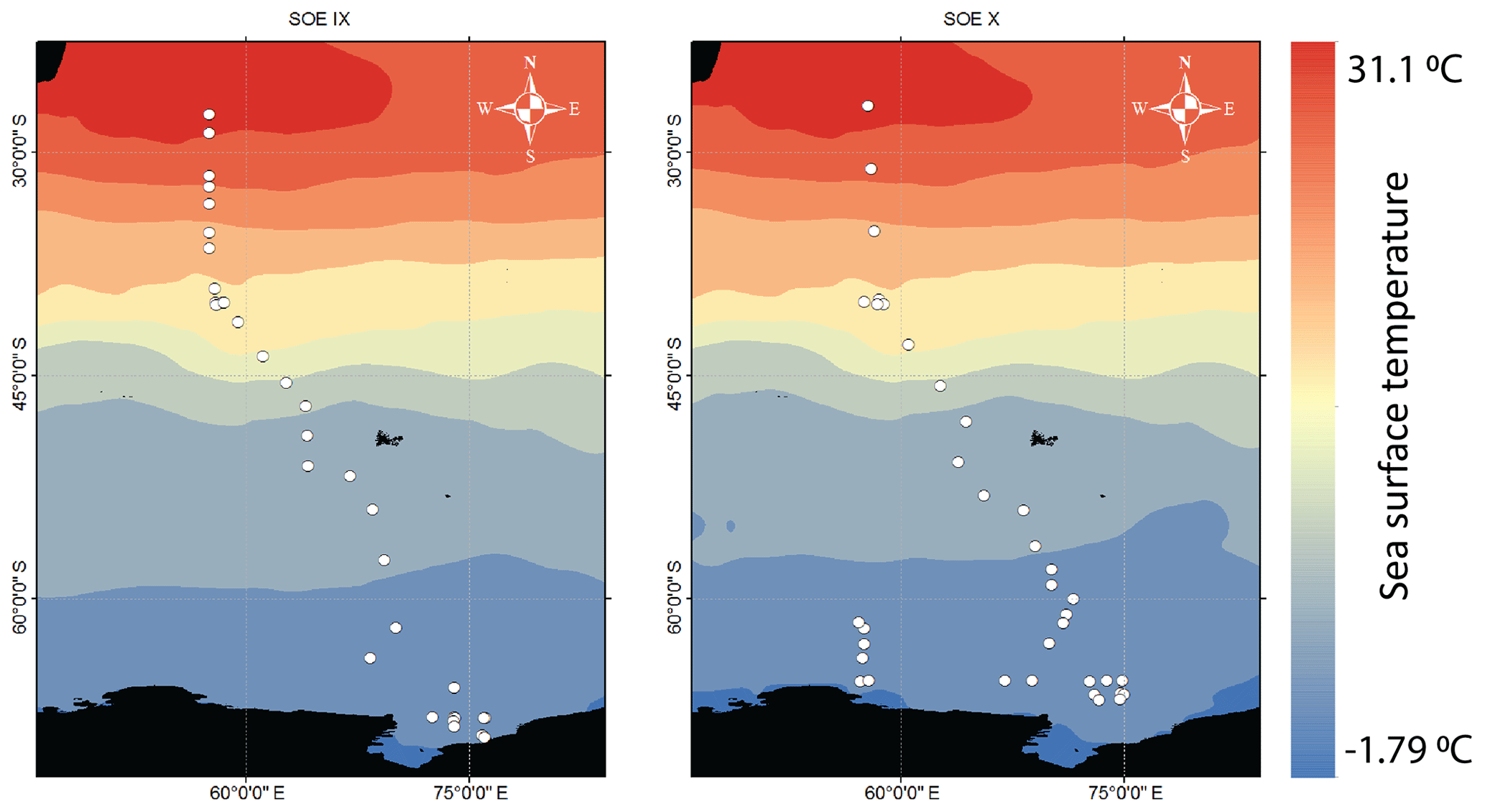
Figure 1 The water vapor sampling locations during the two expeditions – January 2017 (SOE-IX) and December 2017 to January 2018 (SOE-X) – shown as open circles overlain on the map of mean monthly sea surface temperature during the two expeditions. The sea surface temperature data are from the Reanalysis R-2 dataset (Kanamitsu et al., 2002).

Figure 2 Latitudinal variability in measured meteorological parameters, temperature, relative humidity, wind speed and atmospheric pressure. Filled blue diamonds and open circles in the temperature plot represent the sea surface temperature and air temperature, respectively.

In addition to water sampling, relative humidity (RH), wind speed (ws), air temperature (T_a), sea surface temperature (SST) and atmospheric pressure (P) were recorded continuously during the expedition. Figure 2 shows the latitudinal variation in these meteorological parameters. A wide range of these physical conditions are encountered since the sampling encompasses a large latitudinal transect.

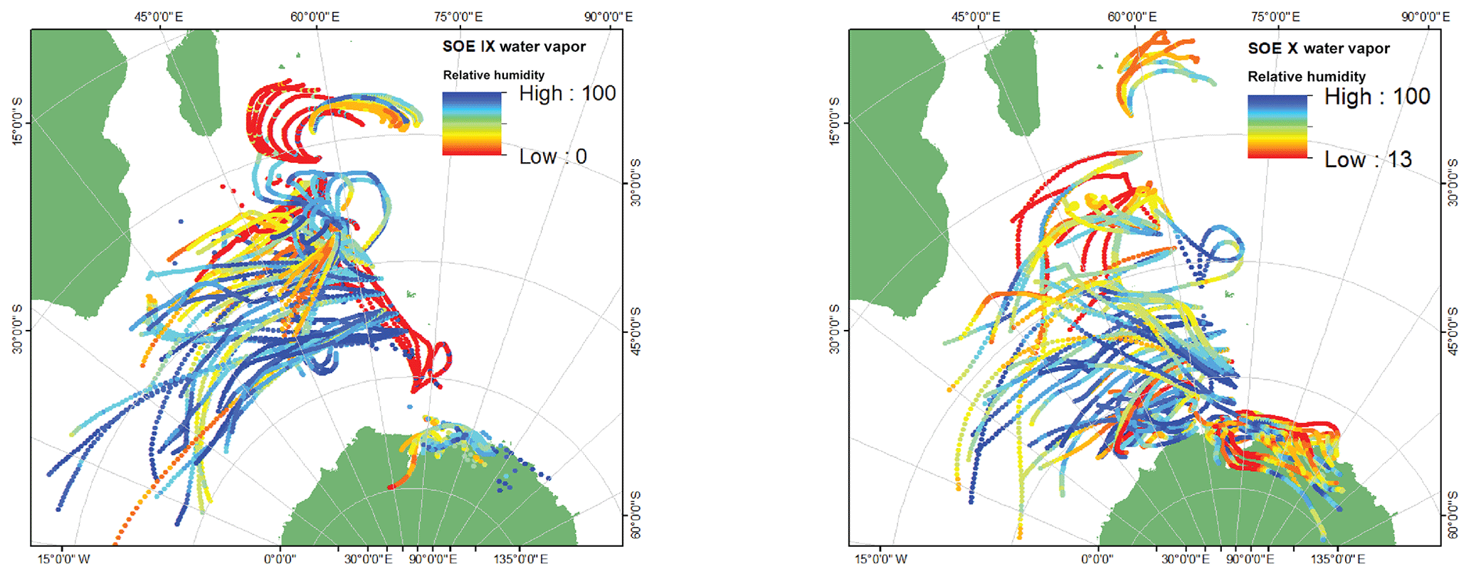
Figure 3 The 72 h back trajectories calculated using HYSPLIT with Reanalysis R-2 data as forcing. The trajectories shown are for three heights: surface, 500 and 1500 m above the mean sea level, and the colors depict the variation in relative humidity along the trajectories.

2.2 Backward air-mass trajectories

In order to reconstruct the vertical profile of the atmospheric moisture transport along the sampling transect, backward air-mass trajectories were generated using the Hybrid Single-Particle Lagrangian Integrated Trajectory (HYSPLIT) model (Draxler and Hess, 1998; Stein et al., 2015) of NOAA–NCEP/NCAR forced with the Reanalysis R-2 data (Kanamitsu et al., 2002). HYSPLIT is a computational model hybrid between Lagrangian and Eulerian methods which generates the paths traversed by the air parcels and calculates meteorological variables such as temperature, relative humidity, specific humidity, rainfall, pressure, etc., along the route. Back trajectories for 3 d are extracted since the average residence time of atmospheric moisture over the oceans is ∼3 d (Trenberth, 1998; Van Der Ent and Tuinenburg, 2017). Figure 3 shows the back trajectories for the water vapor sampling locations. The sampling locations can be broadly categorized into zones which are defined by different wind patterns (i.e., velocity and the moisture carrying capacity). Westerlies and polar easterlies were identified based on these 72 h back trajectories constructed at three different heights above the ocean surface. During the SOE-X expedition, the change in trajectories to westerlies was at ∼31^∘ S. At ∼63^∘ S, change from westerlies to polar easterlies is seen. For SOE-IX the transition from the westerlies to easterlies and then to polar westerlies was documented at the ∼33 and ∼64^∘ S latitudes, respectively.

2.3 The Craig–Gordon models

Craig–Gordon in 1965 (CG; Craig and Gordon, 1965) proposed the first theoretical model to explain the isotopic composition of water vapor during the evaporation process. The isotopic composition of vapor generated on top of the ocean water depends on the isotopic composition of the surface oceanic water, the isotopic composition of water vapor in the ambient atmosphere and the relative humidity at the site of sample collection. The interplay of equilibrium and kinetic fractionation between these phases governs the final isotopic composition in the water vapor and liquid. The equilibrium fractionation between ocean water and vapor is controlled by the sea surface temperature (SST). In comparison, relative humidity and wind speed control the kinetic fractionation through the combination of processes which include both molecular and turbulent diffusion. Molecular diffusion leads to isotopic fractionation between liquid and vapor, whereas the turbulent diffusion is non-fractionating. To estimate the isotopic composition of water vapor, the CG model invokes two layers: a laminar layer above the air–water interface where the transport process is active via molecular diffusion and a turbulent layer above the laminar layer in which the molecular transfer is predominantly by the action of turbulent diffusion. Assuming there is no divergence/convergence of air mass over the oceanic atmosphere, the isotopic ratio of the evaporation flux is given as in Craig and Gordon (1965), referred to as the Traditional Craig–Gordon (TCG) model:

$$\begin{array}{}\text{(1)}& R_{\mathrm{ev}}={\mathit{\alpha }}_{\mathrm{k}}\cdot {\displaystyle \frac{R_{\mathrm{L}}\cdot {\mathit{\alpha }}_{\mathrm{eq}}-\mathrm{RH}\cdot R_{\mathrm{A}}}{\mathrm{1}-\mathrm{RH}}},\end{array}$$

where R_L, R_A, RH, and α_k and α_eq are, respectively, the isotopic composition of the liquid water, the isotopic composition environmental atmospheric moisture, the relative humidity, and the kinetic and the equilibrium fractionation factors. The TCG models in this form and with modifications have been employed in diverse applications and used in numerous studies. The global closure, i.e., assuming a steady state, is achieved in which the isotopic composition of vapor removed from the system has the same composition as atmospheric vapor (Merlivat, 1978):

$$\begin{array}{}\text{(2)}& R_{\mathrm{A}}=R_{\mathrm{ev}}.\end{array}$$

The global closure assumption (Eq. 2) is substituted in Eq. (1) to give

$$\begin{array}{}\text{(3)}& {\displaystyle }{R}_{\mathrm{ev}}={\mathit{\alpha }}_{\mathrm{k}}\cdot {\displaystyle \frac{R_{\mathrm{L}}\cdot {\mathit{\alpha }}_{\mathrm{eq}}-\mathrm{RH}\cdot R_{\mathrm{ev}}}{\mathrm{1}-\mathrm{RH}}}\text{(4)}& {\displaystyle }{R}_{\mathrm{ev}}(\mathrm{1}-\mathrm{RH})={\mathit{\alpha }}_{\mathrm{k}}\cdot \left[R_{\mathrm{L}}\cdot {\mathit{\alpha }}_{\mathrm{eq}}-\mathrm{RH}\cdot R_{\mathrm{ev}}\right]\text{(5)}& {\displaystyle }{R}_{\mathrm{ev}}(\mathrm{1}-\mathrm{RH})+{\mathit{\alpha }}_{\mathrm{k}}\mathrm{RH}\cdot R_{\mathrm{ev}}={\mathit{\alpha }}_{\mathrm{k}}\cdot R_{\mathrm{L}}\cdot {\mathit{\alpha }}_{\mathrm{eq}}\text{(6)}& {\displaystyle }{R}_{\mathrm{ev}}\left[(\mathrm{1}-\mathrm{RH})+{\mathit{\alpha }}_{\mathrm{k}}\cdot \mathrm{RH}\right]={\mathit{\alpha }}_{\mathrm{k}}\cdot R_{\mathrm{L}}\cdot {\mathit{\alpha }}_{\mathrm{eq}}\text{(7)}& {\displaystyle }{R}_{\mathrm{ev}}={\displaystyle \frac{{\mathit{\alpha }}_{\mathrm{eq}}{\mathit{\alpha }}_{\mathrm{k}}{R}_{\mathrm{L}}}{(\mathrm{1}-\mathrm{RH})+{\mathit{\alpha }}_{\mathrm{k}}\cdot \mathrm{RH}}}.\end{array}$$

Recently, Gonfiantini et al. (2018) proposed a modified version of the model, termed as the Unified Craig–Gordon (UCG) model in which the parameters controlling the isotopic composition of the evaporation flux are considered simultaneously. From Gonfiantini et al. (2018), the net evaporation rate of liquid water (E) is the difference between the vaporization rate, ψ_vap, and the atmospheric vapor capture rate (i.e., condensation) by the liquid water, ψ_cap.

$$\begin{array}{}\text{(8)}& E={\mathit{\psi }}_{\mathrm{vap}}-{\mathit{\psi }}_{\mathrm{cap}}=(\mathit{\gamma }-\mathrm{RH}){\mathit{\psi }}_{\mathrm{cap}}^{\mathrm{o}},\end{array}$$

where the ${\mathit{\psi }}_{\mathrm{cap}}^{\mathrm{o}}$ is the vaporization rate of pure water, RH is the relative humidity, and γ is the thermodynamic activity coefficient of evaporating water, which is <1 for the saline solutions and 1 for the pure water or dilute solutions.

Figure 4 (a) Measured δ¹⁸O_sw as black filled circles and values of surface water isotopic composition extracted from the Global Seawater Oxygen-18 Database along the latitudinal transect (open black circles). Also plotted as orange filled squares are the salinity values along the transect. (b) Pink and purple filled diamonds depict the δ¹⁸O_wv of water vapor samples collected during the SOE-IX and SOE-X, respectively, at height of ∼15 m above the water surface. (c) Latitudinal variation in dxs in water vapor samples shown as open red and purple diamonds for SOE-IX and SOE-X, respectively.

From Eq. (8), we can write

$$\begin{array}{}\text{(9)}& {\displaystyle }{R}_{\mathrm{ev}}(\mathit{\gamma }-\mathrm{RH}){\mathrm{\Psi }}_{\mathrm{vap}}^{\mathrm{o}}=R_{\mathrm{esc}}\mathit{\gamma }{\mathrm{\Psi }}_{\mathrm{vap}}^{\mathrm{o}}-R_{\mathrm{cap}}\mathrm{RH}{\mathrm{\Psi }}_{\mathrm{vap}}^{\mathrm{o}}\text{(10)}& {\displaystyle }{R}_{\mathrm{ev}}(\mathit{\gamma }-\mathrm{RH}){\mathrm{\Psi }}_{\mathrm{vap}}^{\mathrm{o}}={\displaystyle \frac{R_{\mathrm{L}}}{{\mathit{\alpha }}_{\mathrm{eq}}{\mathit{\alpha }}_{\mathrm{diff}}^x}}\mathit{\gamma }{\mathrm{\Psi }}_{\mathrm{vap}}^{\mathrm{o}}-{\displaystyle \frac{R_{\mathrm{A}}}{{\mathit{\alpha }}_{\mathrm{diff}}^x}}\mathrm{RH}{\mathrm{\Psi }}_{\mathrm{vap}}^{\mathrm{o}}\text{(11)}& {\displaystyle }{R}_{\mathrm{ev}}={\displaystyle \frac{\frac{R_{\mathrm{L}}}{{\mathit{\alpha }}_{\mathrm{eq}}{\mathit{\alpha }}_{\mathrm{diff}}^x}\mathit{\gamma }-\frac{R_{\mathrm{A}}}{{\mathit{\alpha }}_{\mathrm{diff}}^x}\mathrm{RH}}{\mathit{\gamma }-\mathrm{RH}}},\end{array}$$

where R_L, R_esc, R_cap and R_A are, respectively, the isotopic composition of the liquid water, isotopic composition of vapor escaping to the saturated layer above which is in thermodynamic equilibrium with water, isotopic composition of environmental atmospheric moisture captured by the equilibrium layer and the isotopic composition environmental atmospheric moisture. R_L, R_esc, R_cap and R_A are defined as in Gonfiantini et al. (2018). α_eq is the isotopic fractionation factor between the liquid water and the vapor in the equilibrium layer. α_diff is the isotopic fractionation factor for diffusion in air affecting the vapor escaping from the equilibrium layer and the environmental vapor entering the equilibrium layer; x is the turbulent index of atmosphere. Introducing the global closure assumption, Eq. (2), in Eq. (11) gives

$$\begin{array}{}\text{(12)}& {\displaystyle }{R}_{\mathrm{ev}}={\displaystyle \frac{\frac{R_{\mathrm{L}}}{{\mathit{\alpha }}_{\mathrm{eq}}{\mathit{\alpha }}_{\mathrm{diff}}^x}\mathit{\gamma }-\frac{R_{\mathrm{ev}}}{{\mathit{\alpha }}_{\mathrm{diff}}^x}\mathrm{RH}}{\mathit{\gamma }-\mathrm{RH}}}\text{(13)}& {\displaystyle }{R}_{\mathrm{ev}}(\mathit{\gamma }-\mathrm{RH})={\displaystyle \frac{R_{\mathrm{L}}}{{\mathit{\alpha }}_{\mathrm{eq}}{\mathit{\alpha }}_{\mathrm{diff}}^x}}\mathit{\gamma }-{\displaystyle \frac{R_{\mathrm{ev}}}{{\mathit{\alpha }}_{\mathrm{diff}}^x}}\mathrm{RH}\text{(14)}& {\displaystyle }{R}_{\mathrm{ev}}(\mathit{\gamma }-\mathrm{RH})+{\displaystyle \frac{R_{\mathrm{ev}}}{{\mathit{\alpha }}_{\mathrm{diff}}^x}}\mathrm{RH}={\displaystyle \frac{R_{\mathrm{L}}}{{\mathit{\alpha }}_{\mathrm{eq}}{\mathit{\alpha }}_{\mathrm{diff}}^x}}\mathit{\gamma }\text{(15)}& {\displaystyle }{R}_{\mathrm{ev}}\left[(\mathit{\gamma }-\mathrm{RH})+{\displaystyle \frac{\mathrm{RH}}{{\mathit{\alpha }}_{\mathrm{diff}}^x}}\right]={\displaystyle \frac{R_{\mathrm{L}}}{{\mathit{\alpha }}_{\mathrm{eq}}{\mathit{\alpha }}_{\mathrm{diff}}^x}}\mathit{\gamma }\text{(16)}& {\displaystyle }{R}_{\mathrm{ev}}\left[{\displaystyle \frac{(\mathit{\gamma }-\mathrm{RH}){\mathit{\alpha }}_{\mathrm{diff}}^x+\mathrm{RH}}{{\mathit{\alpha }}_{\mathrm{diff}}^x}}\right]={\displaystyle \frac{R_{\mathrm{L}}}{{\mathit{\alpha }}_{\mathrm{eq}}{\mathit{\alpha }}_{\mathrm{diff}}^x}}\mathit{\gamma }\text{(17)}& {\displaystyle }{R}_{\mathrm{ev}}={\displaystyle \frac{R_{\mathrm{L}}}{{\mathit{\alpha }}_{\mathrm{eq}}{\mathit{\alpha }}_{\mathrm{diff}}^x}}\mathit{\gamma }\left[{\displaystyle \frac{{\mathit{\alpha }}_{\mathrm{diff}}^x}{(\mathit{\gamma }-\mathrm{RH}){\mathit{\alpha }}_{\mathrm{diff}}^x+\mathrm{RH}}}\right]\text{(18)}& {\displaystyle }{R}_{\mathrm{ev}}={\displaystyle \frac{R_{\mathrm{L}}\mathit{\gamma }}{{\mathit{\alpha }}_{\mathrm{eq}}\left[{\mathit{\alpha }}_{\mathrm{diff}}^x(\mathit{\gamma }-\mathrm{RH})+\mathrm{RH}\right]}}.\end{array}$$

The temperature-dependent equilibrium fractionation factor is calculated using the formulation given by Horita and Wesolowski (1994). The kinetic factor takes into account diffusion in air affecting the vapor escaping from the equilibrium layer and is controlled by α_diff, which is the molecular diffusivity of the different isotopologues of water. Molecular diffusivities (${\mathit{\alpha }}_{\mathrm{diff}}^{\mathrm{O}}$, ${\mathit{\alpha }}_{\mathrm{diff}}^{\mathrm{H}}$) data are taken from three previous studies Merlivat (1978) (1.0285, 1.0251), Cappa et al. (2003) (1.0318, 1.0164) and Pfahl and Wernli (2009) (1.0076, 1.0039) referred to as MJ, CD and PW, respectively. x is the turbulence index of atmosphere, which signifies the proportion of vapor that escapes by isotopic fractionating molecular diffusion and non-fractionating turbulent diffusion. When x=1 the vapor escapes solely by molecular diffusion, and for x=0 the vapor escapes only due to turbulent diffusion.

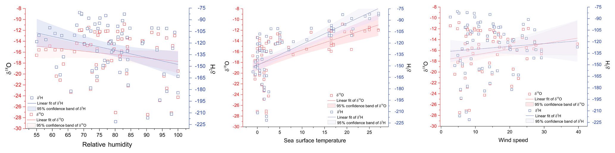
Figure 5 Linear regression for isotopic composition of water vapor and physical parameters (sea surface temperature, relative humidity and wind speed). Hollow red and blue squares represent the δ¹⁸O and δ²H, respectively, and the shaded areas depict the 95 % confidence bands. The linear regression lines are shown as blue and red for δ²H and δ¹⁸O, respectively. The slope and intercept of the linear regression equations along with data from Uemura et al. (2008) are listed in Tables S1 and S2.

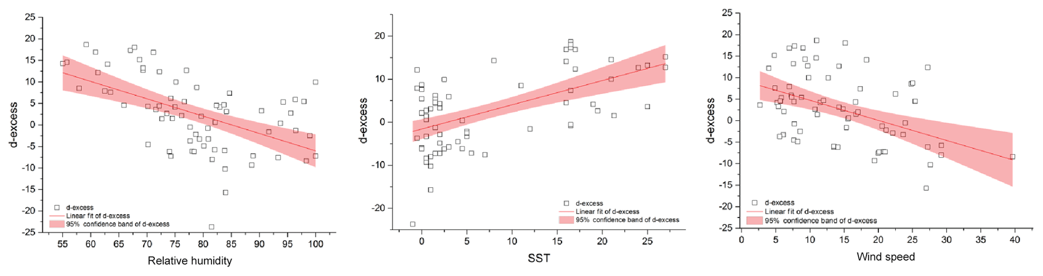
Figure 6 Regression plots for d-excess (hollow black squares) in water vapor and the meteorological conditions (relative humidity, sea surface temperature and wind speed). The shaded region depicts the 95 % confidence bands of d-excess. The slope and intercept of the regression equations along with data from Uemura et al. (2008) are listed in Table 2.

3 Results

3.1 Isotopic measurements along the transect

δ¹⁸O of surface water was >0 ‰ until ∼40^∘ S latitude. A transition to lighter isotopic composition was observed beyond ∼45^∘ S latitude with a drop documented in the surface water isotopic values on approaching the coastal Antarctic regions. Figure 4a shows the latitudinal variation in δ¹⁸O_sw, plotted along with salinity values measured along the transect. In addition, the δ¹⁸O values of ocean surface water extracted from the Global Seawater Oxygen-18 Database (SWD) (Schmidt et al., 1999) are also plotted. There is a mismatch between the observed depleted isotopic values near coastal Antarctica and the SWD values. The SWD is a surface interpolated dataset based on point observations in the global ocean. This is probably one of the major causes of the difference, the others being the season or the month of sample collection.

The δ¹⁸O_wv and δ²H_wv in water vapor samples showed a consistent trend across latitudes for both the expeditions. The δ¹⁸O_wv (δ²H_wv) of water vapor varies from −10.9 ‰ (−80.8 ‰) to −27.5 ‰ (−221.4 ‰), respectively. The vapor isotopic composition is seen to be gradually decreasing with lighter isotopic values at higher latitudes. A steady drop was noted from ∼30 to ∼65^∘ S and a sharp change in the gradient was registered at ∼65^∘ S. Extreme lighter values recorded on approaching ∼65^∘ S are attributed to factors such as low temperature and the mixing of lighter vapor from continental Antarctica (Uemura et al., 2008). There are deviations from this general trend with heavier isotopic composition observed at the higher latitudes or vice versa. These variations can be accounted for by taking into consideration the source and the path of air masses. The lighter (heavier) values of vapor isotopic composition can be traced to the source being lower (higher) latitudes.

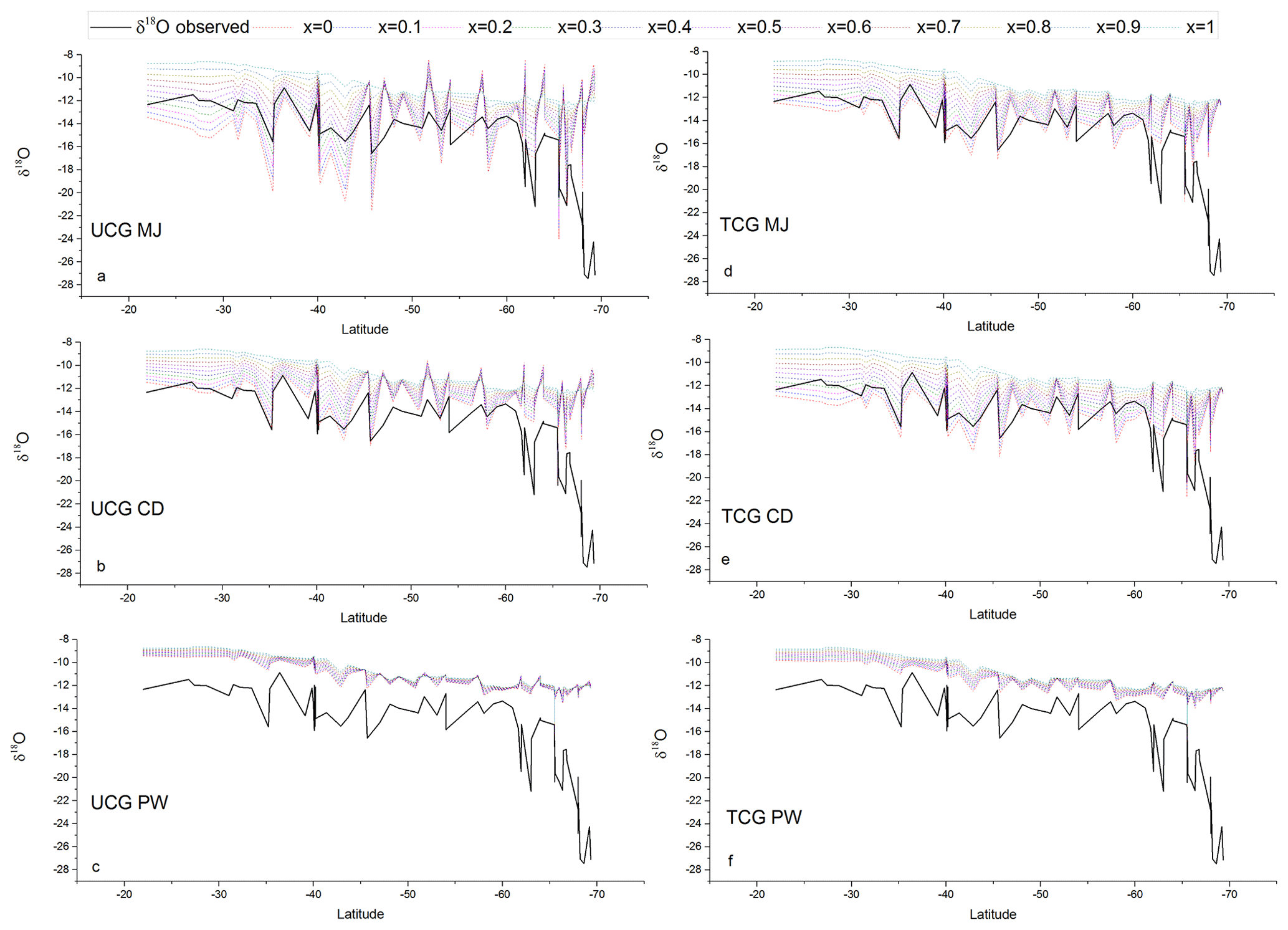
Figure 7 Comparison between the latitudinal distribution of the measured water vapor δ¹⁸O (black lines) and that predicted by the TCG and UCG models, employing the global closure assumption for different molecular diffusivity ratios and turbulence indices, shown as colored lines.

Deuterium excess (d-excess or dxs), defined as $\text{d-excess}={\mathit{\delta }}^{\mathrm{2}}\mathrm{H}-\mathrm{8}\times {\mathit{\delta }}^{\mathrm{18}}\mathrm{O}$, is a second-order isotope parameter, which is a measure of kinetic fractionation during evaporation (Dansgaard, 1964). The d-excess in the water vapor correlates with meteorological parameters at the ocean surface such as relative humidity, sea surface temperature and wind speed (Uemura et al., 2008; Rahul et al., 2018; Benetti et al., 2014; Midhun et al., 2013). Therefore, it serves as a proxy for the moisture source conditions in the evaporation regions. The dxs and relative humidity are strongly coupled, which is determined by the magnitude of moisture gradient between evaporating water surface and overlying unsaturated air. In other words, the lower the relative humidity, the higher the dxs in the overlying moisture. Wind speed regulates the turbulent vs. molecular diffusion across the diffusive layer. The role of SST in governing the dxs is through the process of equilibrium fractionation, which is temperature dependent. The dxs values in water vapor samples range from 18.7 ‰ to −23.7 ‰. A relatively higher dxs value in the water vapor from ∼25 to ∼45^∘ S with a slight step change to lower dxs values was recorded on approaching 45^∘ S, which extends until ∼65^∘ S. Beyond ∼65^∘ S, a slight increment in the vapor dxs was observed. The very low dxs values can be attributed to the mixing of vapor evaporated from sea spray under high-wind-speed conditions are observed during the passage of extratropical cyclones. The statistics of the isotopic composition of water vapor are tabulated in Table 1.

Table 1 Descriptive statistics of the water vapor isotopic composition.

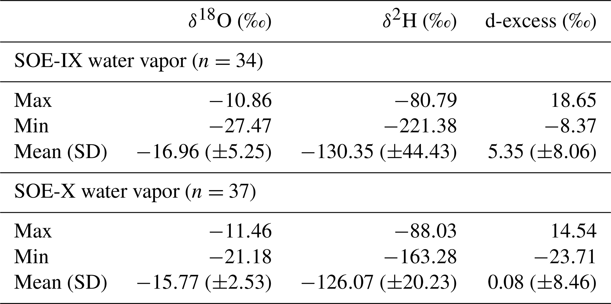
Figure 8 Comparison between the latitudinal distribution of the measured d-excess in water vapor (black lines) and that predicted by the TCG and UCG models, employing the global closure assumption for different molecular diffusivity ratios and turbulence indices, shown as colored lines.

3.2 Meteorological controls on the isotopic composition of water vapor

The δ¹⁸O_wv and δ²H_wv are positively correlated with SST, negatively correlated with wind speed and uncorrelated with relative humidity. For all the water vapor samples, δ²H_wv and δ¹⁸O_wv are correlated with SST, explaining ∼33 % of the variance in δ¹⁸O_wv and ∼50 % of the variance in δ²H_wv. The correlation coefficient is higher if sampling from individual years is considered separately. In all cases, the slope and intercept of the regression equation between the isotopic composition of water vapor and SST are comparable with previous observations from the Southern Ocean (Uemura et al., 2008). The linear regression plots are shown in Fig. 5, and the regression parameters (slope, intercept, standard errors and r²) for δ¹⁸O and δ²H are listed in Tables S1 and S2 in the Supplement, respectively. The regression equations are calculated for different sample classifications, with and without the influence of Antarctic vapor mixing as evident from the back trajectories (i.e., samples collected north of 65^∘ S) and for individual expeditions.

Table 2 Slope, intercept and r² of the linear regression equations between meteorological parameters (relative humidity, sea surface temperature and winds speed) and d-excess for different sample classifications. Also listed are the regression parameters for the data from Uemura et al. (2008).

Figure 6 shows the regression plots of dxs in vapor with the meteorological conditions, and the parameters defining the regression equations are listed in Table 2. For samples collected north of 65^∘ S, the linear regression equation describing the relationship between dxs and relative humidity is $\mathrm{dxs}=-\mathrm{0.56}\mathrm{RH}+\mathrm{46.36}$ (r²=0.49). These slope and intercept values are similar to the earlier records, documenting the isotope variability in water vapor from the Southern Ocean (Uemura et al., 2008; Rahul et al., 2018) the Bay of Bengal (Midhun et al., 2013), the Atlantic (Benetti et al., 2014) and the Mediterranean (Gat et al., 2003). For samples collected south of 65^∘ S the relationship becomes weaker. The strength of the dxs vs. RH relationship was stronger if data exclusively from the expeditions are considered separately, for SOE-IX and SOE-X as $\mathrm{dxs}=-\mathrm{0.64}\mathrm{RH}+\mathrm{57.4}$ (r²=0.77) and $\mathrm{dxs}=-\mathrm{0.64}\mathrm{RH}+\mathrm{48.7}$ (r²=0.61), respectively. Collectively for both the expeditions, the dxs in vapor is positively correlated with the SST, and the regression parameters are comparable with those from previous observations in the Southern Ocean and also for the Atlantic Ocean and the Bay of Bengal. For SST vs. dxs, the linear regression equation for samples collected north of 65^∘ S is given by $\mathrm{dxs}=\mathrm{0.70}\mathrm{SST}-\mathrm{4.65}$ (r²=0.49). The dxs of water vapor samples are negatively correlated with wind speed. For samples collected north of 65^∘ S the correlation the regression equation is given by $\mathrm{dxs}=-\mathrm{0.53}\mathrm{ws}+\mathrm{11.65}$ (r²=0.23). Our observation is consistent with the earlier studies suggesting the dependency of water vapor d-excess on relative humidity, SST and wind speed.

4 Discussion

4.1 Craig–Gordon (CG) model evaluation

The isotopic composition of evaporation flux from the oceans is calculated using the CG models (TCG and UCG) assuming three molecular diffusivity ratios driving the kinetic fractionation and for varied contribution of turbulent vs. molecular diffusion-enabled transport factors. The simulated values of the isotopic composition of evaporation flux with these different models under the global closure assumption are compared with the measured isotopic values of water vapor over the ocean. The model and the constraints that best describe the observations are selected based on the model-predicted and observed relationships between the dxs of water vapor and physical parameters (SST, ws and RH).

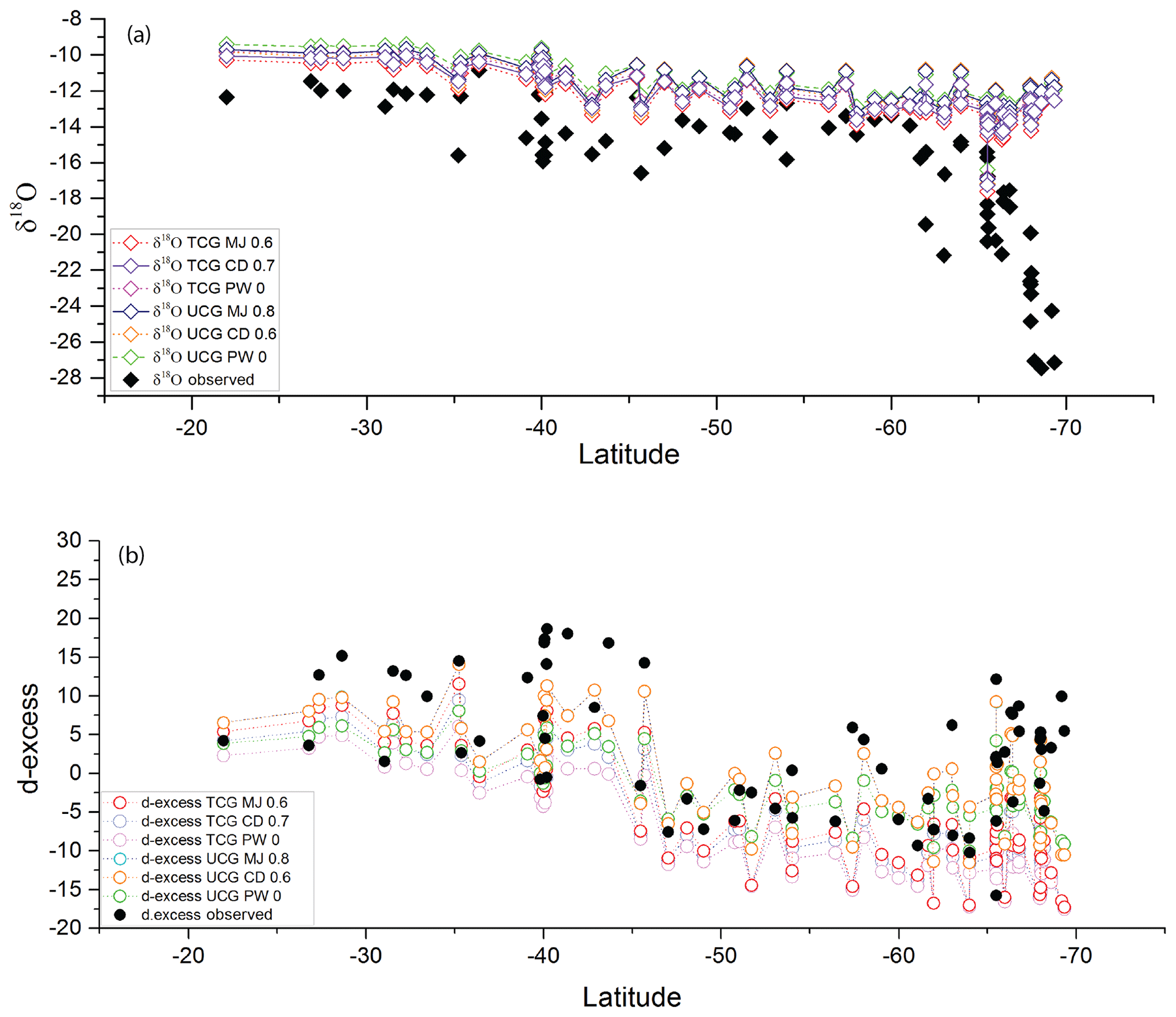
Figure 9 Latitudinal variation in the observed (a) δ¹⁸O as filled black diamonds and (b) d-excess as filled black circles and the modeled values (colored open diamonds and circles) for the model runs where the observed slope is comparable to the modeled slope. The statistical parameters analysis of the observed and modeled regression are listed in Table 3.

The TCG and the UCG models are run for MJ, CD and PW molecular diffusivities and for the turbulence index of the atmosphere varying from 0 to 1, with an increment of 0.1. Figures 7 and 8 show the comparison between the TCG and UCG modeled vapor isotopic composition (δ¹⁸O and d-excess) with the observations. There are values for the turbulence index (x) of the atmosphere where model-predicted δ¹⁸O and d-excess overlap with the observations for both TCG and UCG models with MJ and CD molecular diffusivity ratios. However, there is a clear mismatch between the model-predicted δ¹⁸O and d-excess for the recommended PW molecular diffusivities in both UCG and TCG models. Another noteworthy feature of the plots is that for all the model runs, a large difference is seen between the modeled and observed isotopic composition for water vapor samples collected south of ∼65^∘ S latitudes, and the best match is seen for samples collected north of ∼65^∘ S. This difference is attributed to the advection and mixing of lighter Antarctic moisture to local moisture for samples collected beyond ∼65^∘ S.

To evaluate the performance of the prediction by these models and identify the parameters that best describe the observations, the slope of the dxs vs. relative humidity predicted by the different model runs is compared with the observed relationships documented based on actual data on samples collected north of 65^∘ S. Figure S1 depicts the comparison between the observed and the model-predicted relationships. The UCG models and the parameters that match the observed slope of the relative humidity vs. d-excess relationship ($-\mathrm{0.56}\pm \mathrm{0.08}$) are ${\mathrm{UCG}}_{x=\mathrm{0.8}}^{\mathrm{MJ}}$, ${\mathrm{UCG}}_{x=\mathrm{0.6}}^{\mathrm{CD}}$ and ${\mathrm{UCG}}_{x=\mathrm{0}}^{PW}$. Similarly for the TCG models ${\mathrm{TCG}}_{x=\mathrm{0.6}}^{\mathrm{MJ}}$, ${\mathrm{TCG}}_{x=\mathrm{0.7}}^{\mathrm{CD}}$ and ${\mathrm{TCG}}_{x=\mathrm{0}}^{PW}$ predict the slopes that are comparable with the observed value. The δ¹⁸O and d-excess of predicted by these models are plotted with the observations in Fig. 9.

Figure 10 Differences between observed and predicted slopes and intercepts of the relationships between d-excess vs. relative humidity, sea surface temperature and wind speed.

Table 3 Slope, intercept and r² of the linear regression equations between observed and modeled δ¹⁸O and d-excess for the best-fit models for samples collected north of 65^∘ S.

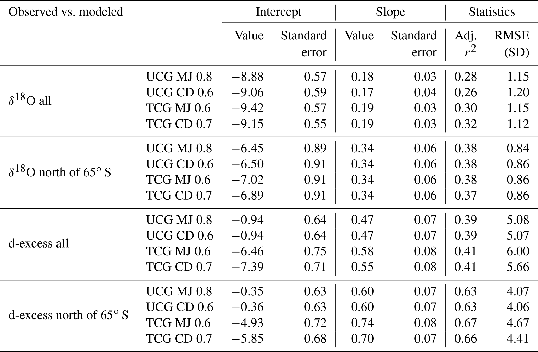
The consistency of model results and observations is best described using a linear regression equation which links model-predicted d-excess and the meteorological parameters (relative humidity, sea surface temperature and wind speed). These regression plots are displayed in Fig. S2. The differences between the model-predicted and the observed values of slopes and intercepts are shown in Fig. 10. The largest difference between the observed and model-predicted slopes and intercepts are for the PW molecular diffusivities for both UCG and the TCG models and therefore excluded from further discussion. For the dxs vs. relative humidity relationship, ${\mathrm{UCG}}_{x=\mathrm{0.8}}^{\mathrm{MJ}}$ and ${\mathrm{UCG}}_{x=\mathrm{0.6}}^{\mathrm{CD}}$ show the smallest difference between the observed and modeled slopes and intercepts followed by ${\mathrm{TCG}}_{x=\mathrm{0.6}}^{\mathrm{MJ}}$ and ${\mathrm{TCG}}_{x=\mathrm{0.7}}^{\mathrm{CD}}$. In case of dxs vs. SST relationship, the TCG models show the least difference between the slopes, and the UCG model predicts the intercept values that are consistent with the observations. Similarly, for the and dxs vs. ws relationships, the UCG and the TCG models produce the values that predict the slope and the intercept values with the least deviation from the observed values. The models that best describe the slope and intercept values of the linear regression equation defining the d-excess vs. the meteorological parameters, the root mean square error of the modeled vs. observed δ¹⁸O and d-excess are listed in Table 3. The ability of the models to predict the δ¹⁸O and d-excess are better demonstrated by the water vapor samples which were collected north of 65^∘ S. The models predict the d-excess with a better correlation than δ¹⁸O, and the TCG model shows a slightly higher possibility to predict the d-excess values than the UCG model.

4.2 Understanding the equilibrium/disequilibrium

The isotopic composition of water vapor over the ocean is governed by the equilibrium and kinetic processes which are defined by the meteorological condition. However, considering only these factors is insufficient to explain the observed variation in the isotopic composition of vapor on top of the ocean. Advective mixing of transported vapor to the locally generated vapor is important and needs to be taken into consideration. Figure 11a shows the difference between the δ¹⁸O and δ²H isotopic composition of vapor (at equilibrium with ocean surface water) and the observed vapor isotopic composition. Kinetic fractionation can explain a part of the departure from the equilibrium state and is evaluated based on the Craig–Gordon models as described in the previous section ($E_{\mathrm{UCG}}^{\mathrm{MJ},\mathrm{0.8}},E_{\mathrm{UCG}}^{\mathrm{CD},\mathrm{0.6}},E_{\mathrm{TCG}}^{\mathrm{MJ},\mathrm{0.6}}$ and $E_{\mathrm{TCG}}^{\mathrm{CD},\mathrm{0.7}}$). The difference between isotopic composition of equilibrium vapor (δ¹⁸O and δ²H) and the modeled isotopic composition of E_UCG and E_TCG is also plotted in Fig. 11b–e. In order to calculate the fractional contribution of the local and advected moisture along the sampling transect, a two-component mixing framework is invoked. The local end member is based on the isotopic composition of vapor predicted by the best match UCG and the TCG model-predicted parameters. The calculations are done assuming the isotopic composition of the advected vapor due to westerlies similar to the earlier proposition (Uemura et al., 2008) (δ²H $\sim -\mathrm{109}$ ‰) in the region between 31 to 65^∘ S. For samples collected in the polar ocean south of 65^∘ S, the temperature plays the role of limiting the local evaporation process, and hence the large differences from the equilibrium conditions can be explained by invoking the process of mixing of Antarctic vapor which is transported to this region by the interplay of polar easterlies. The average isotopic composition of water vapor collected at the Dome C site (December 2014–January) (Wei et al., 2019) (${\mathit{\delta }}^{\mathrm{2}}\mathrm{H}=-\mathrm{490}\pm \mathrm{23}$ ‰) is chosen as representative of the advected vapor transported by the polar easterlies. It is seen that in order to explain the water vapor isotope ratio observation over the ocean south of 65^∘ S, the contribution of lighter Antarctic vapor is expected. Figure 12b shows the relative contribution of advected and locally generated moisture in our observation. The advected component is a prominent component of the ambient vapor on approaching higher latitudes. South of 65^∘ S the amount of moisture present in the atmosphere is less and is largely local in origin with a small mixing of lighter Antarctic vapor. However, the contribution of the Antarctic vapor linearly increases on approaching the coastal regions.

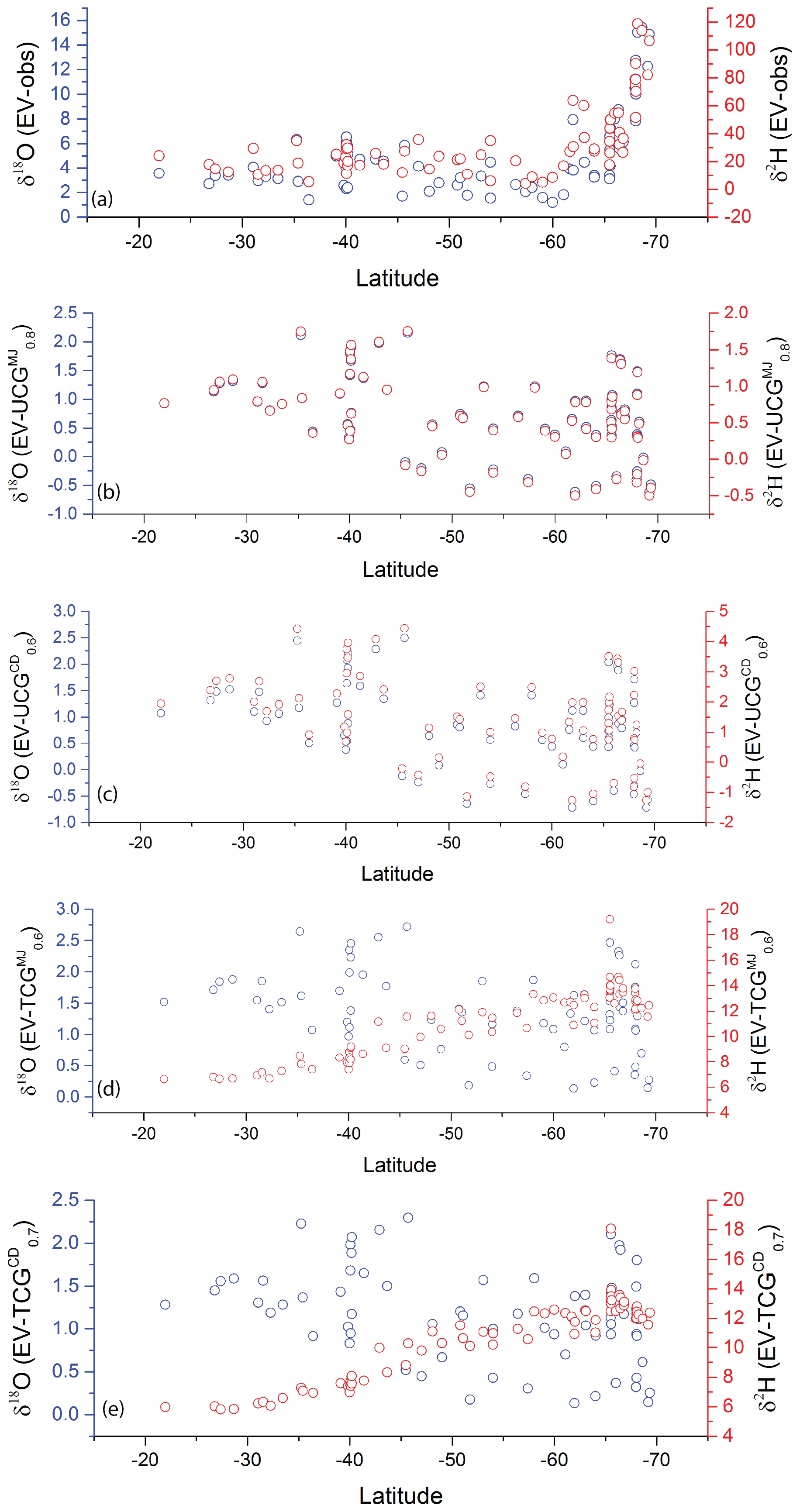
Figure 11 (a) The difference between the δ¹⁸O (blue columns) and δ²H (red open circles) of equilibrium vapor and observed water vapor isotopic composition. Panels (b)–(e) show the difference between the δ¹⁸O and δ²H equilibrium vapor and that predicted by the best-fit model runs.

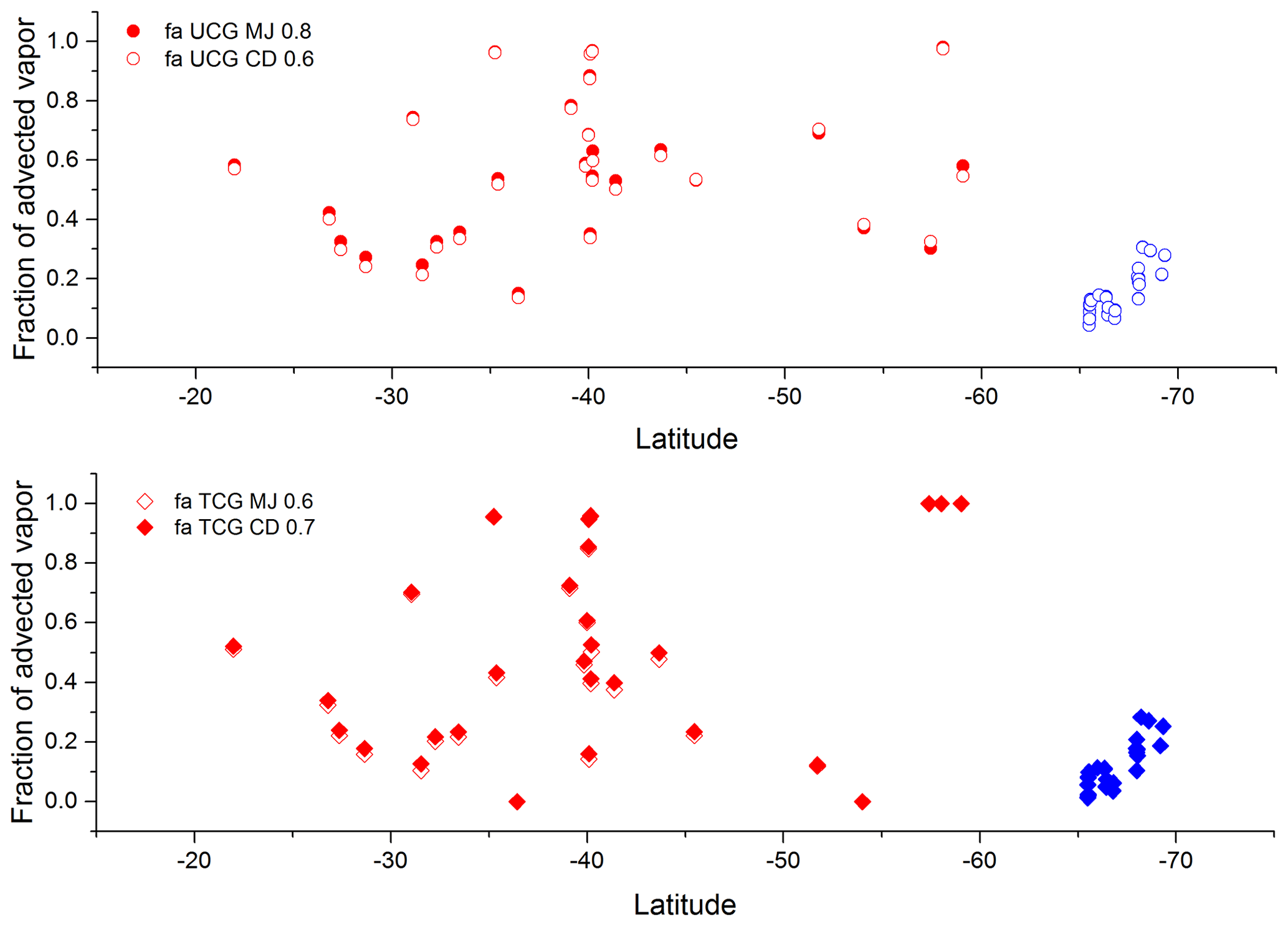
Figure 12 Fraction of advected vapor that explains the water vapor isotopic composition for the best-fit model runs. Red and blue colors depict the different end-member compositions used for calculations.

5 Conclusions

In this study, the isotopic composition of water vapor and surface water samples collected across a latitudinal transect from Mauritius to Prydz Bay in the Southern Ocean are described. The isotopic composition of evaporating vapor is governed by the isotopic composition of the water, ambient vapor isotopic composition, exchange and mixing processes at the water–air interface, and the local meteorological conditions. These controlling parameters were considered separately or simultaneously for explaining the observation best quantifying the evaporation mechanism adopted in the Craig–Gordon models. The Traditional Craig–Gordon (Craig and Gordon, 1965) (TCG) and the Unified Craig–Gordon (UCG) (Gonfiantini et al., 2018) equations were used to predict the isotopic composition of evaporation flux after incorporating different molecular diffusivity ratios at varying fractions of molecular and turbulent diffusion. The best match between the modeled and observed values is seen by using the MJ and CD molecular diffusivity ratios, whereas the largest mismatch occurs for the PW values of the molecular diffusivities. The results ascertain the importance of the fraction of molecular vs. turbulent fraction (i.e., isotopically fractionating vs. non fractionating exchange) used to predict the isotopic composition of the evaporation flux in these Craig–Gordon models. ${\mathrm{UCG}}_{x=\mathrm{0.8}}^{\mathrm{MJ}}$, ${\mathrm{UCG}}_{x=\mathrm{0.6}}^{\mathrm{CD}}$, ${\mathrm{TCG}}_{x=\mathrm{0.6}}^{\mathrm{MJ}}$ and ${\mathrm{TCG}}_{x=\mathrm{0.7}}^{\mathrm{CD}}$ models predicted the slope and the intercepts of dxs vs. meteorological parameters with an appreciable accuracy and consistent with the observations. The remaining difference between the observed and simulated isotopic composition of water vapor is explained by incorporating an advective framework where the advected vapor mass is assumed to mix with the locally generated vapor in a mixing model. The assignment of the advective component is based on the path followed by the air-masses calculated by the HYSPLIT trajectory model. The relative contribution of advected and locally evaporated fluxes was estimated by assigning end-member isotopic composition and solving in a two-component mixing framework. The approximation of the locally generated end-member composition is based on ${\mathrm{UCG}}_{x=\mathrm{0.8}}^{\mathrm{MJ}}$, ${\mathrm{UCG}}_{x=\mathrm{0.6}}^{\mathrm{CD}}$, ${\mathrm{TCG}}_{x=\mathrm{0.6}}^{\mathrm{MJ}}$ and ${\mathrm{TCG}}_{x=\mathrm{0.7}}^{\mathrm{CD}}$. The advected moisture flux is assigned values based on the origin and path followed by the back trajectories. It is found that beyond 65^∘ S latitude, lighter isotope values observed in the water can be explained by invoking mixing of Antarctic vapor, with its contribution linearly increasing towards the coast.

Although the advective model can explain the water vapor composition along the transect, nonetheless there can be other sources of advective humidity to the atmospheric boundary layer such as from upper-atmospheric layers with different properties, vapor generated from the re-evaporation of rainfall, evaporation of sea spray, or sublimation of snow and ice. These processes may occur under conditions which are not possible to take into account due the cryogenic sampling method for collection of water vapor used in this study. The study can be improved and by measuring the water vapor isotopic composition continuously along the transect using a infrared laser spectrometer and conducting a high-resolution precipitation sampling during the passage of extratropical cyclones.