The incorporation of the Tripleclouds concept into the δ-Eddington two-stream radiation scheme: solver characterization and its application to shallow cumulus clouds

The treatment of unresolved cloud–radiation interactions in weather and climate models has considerably improved over the recent years, compared to conventional plane-parallel radiation schemes, which previously persisted in these models for multiple decades. One such improvement is the state-of-the-art Tripleclouds radiative solver, which has one cloud-free and two cloudy regions in each vertical model layer and is thereby capable of representing cloud horizontal inhomogeneity. Inspired by the Tripleclouds concept, primarily introduced by Shonk and Hogan (2008), we incorporated a second cloudy region into the widely employed δ-Eddington two-stream method with the maximum-random overlap assumption for partial cloudiness. The inclusion of another cloudy region in the two-stream framework required an extension of vertical overlap rules. While retaining the maximum-random overlap for the entire layer cloudiness, we additionally assumed the maximum overlap of optically thicker cloudy regions in pairs of adjacent layers. This extended overlap formulation implicitly places the optically thicker region towards the interior of the cloud, which is in agreement with the core–shell model for convective clouds. The method was initially applied on a shallow cumulus cloud field, evaluated against a three-dimensional benchmark radiation computation. Different approaches were used to generate a pair of cloud condensates characterizing the two cloudy regions, testing various condensate distribution assumptions along with global cloud variability estimate. Regardless of the exact condensate setup, the radiative bias in the vast majority of Tripleclouds configurations was considerably reduced compared to the conventional plane-parallel calculation. Whereas previous studies employing the Tripleclouds concept focused on researching the top-of-the-atmosphere radiation budget, the present work applies Tripleclouds to atmospheric heating rate and net surface flux. The Tripleclouds scheme was implemented in the comprehensive libRadtran radiative transfer package and can be utilized to further address key scientific issues related to unresolved cloud–radiation interplay in coarse-resolution atmospheric models.

1 Introduction

Radiation schemes in coarse-resolution numerical weather prediction and climate models, commonly referred to as general circulation models (GCMs), have traditionally been claimed to be impaired by the poor representation of clouds (Randall et al., 1984, 2003, 2007). Undoubtedly, one of the most rigorous assumptions that persisted in GCMs for multiple decades, was the complete removal of cloud horizontal heterogeneity – the so-called plane-parallel cloud representation (Fig. 1d). Since the nature of cloud–radiation interactions is intrinsically nonlinear, the plane-parallel representation of clouds leads to substantial biases of GCM radiative quantities (Cahalan et al., 1994a, b; Cairns et al., 2000). Further, an assumption of how partial cloudiness vertically overlaps within each GCM grid column is required. The widely employed assumption is the maximum-random overlap (Geleyn and Hollingsworth, 1979), advocated by many studies (e.g., Tian and Curry, 1989) and recently criticized by others, since it breaks down in the case of vertically developed cloud systems in strongly sheared environments (e.g., Hogan and Illingworth, 2000; Naud et al., 2008; Di Giuseppe and Tompkins, 2015). Last but not least, three-dimensional (3-D) radiative effects related to subgrid horizontal photon transport, which in reality manifests itself most pronouncedly in regions characterized by strong horizontal gradients of optical properties, such as cloud side boundaries (Jakub and Mayer, 2015, 2016; Klinger and Mayer, 2014, 2016), are currently still neglected in the majority of GCMs. This broad palette of issues is challenging to tackle and solve.

In order to reduce the most striking plane-parallel biases, several methods were developed in the past. The scaling factor method, proposed by Cahalan et al. (1994a) and implemented in the ECMWF model by Tiedtke (1996), was a conventional approach, where the cloud optical depth was multiplied by a constant factor and the resulting effective optical depth was passed to the radiation scheme. Oreopoulos et al. (1999) introduced a more sophisticated gamma-weighted radiative transfer scheme, later also applied by Carlin et al. (2002) and Rossow et al. (2002), where the optical depth across a grid box is weighted using a gamma distribution. Moreover, Barker et al. (2002) and subsequently Pincus et al. (2003) presented an alternative technique, known as the Monte Carlo integration of independent column approximation (McICA; Fig. 1e), which is currently operationally employed in most large-scale atmospheric models. The fundamental assumption of the McICA is that the independent column approximation (ICA; Fig. 1c) is adequate and therefore allows for the independent generation of subgrid cloudy columns, which is managed by means of stochastic cloud generator (Räisänen et al., 2004; Räisänen and Barker, 2004). As the full ICA is not affordable within the computational constraints of simulating complex weather and climate scenarios, the computing speed gain in the McICA approach is based on the simultaneous sampling of subgrid cloud state and spectral interval.

Whereas all aforementioned methodologies certainly brought improvements compared to the conventional plane-parallel cloud representation, they all have some disadvantages. The usage of the McICA, for example, introduces conditional random errors (the McICA noise) to radiative quantities, and it is unclear how significantly this affects the forecast skill. Räisänen et al. (2007), as an illustration, investigated the impact of the McICA noise in an atmospheric GCM (ECHAM5; Roeckner et al., 2003) and found statistically discernible impacts on simulated climate for a fairly reasonable McICA implementation. The largest effect was observed in the boundary layer, where clouds are essentially maintained by local cloud-top radiative cooling. As the McICA noise disrupted this cooling, a positive feedback loop was induced, where a reduction of cloud fraction led to weaker radiative cooling, which in turn further diminished the cloud fraction. Similar findings were already previously reported by Räisänen et al. (2005) for global climate simulated with another GCM.

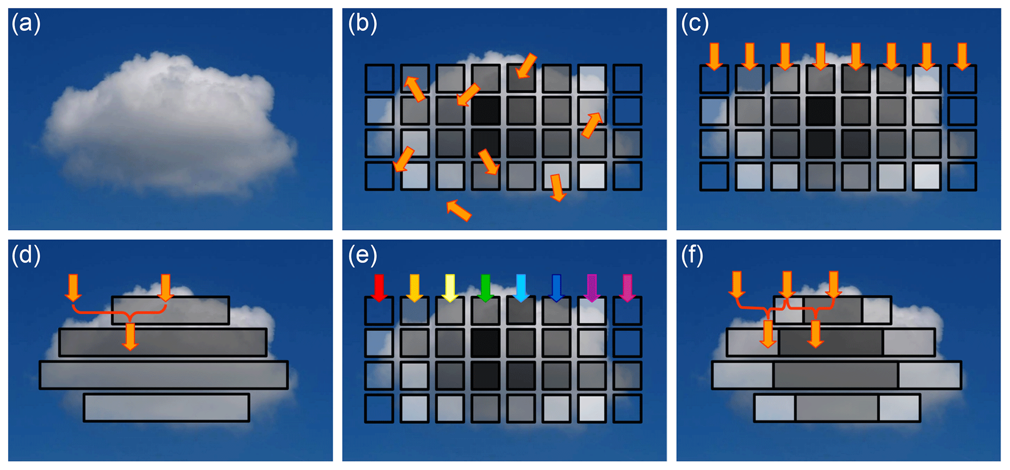
Figure 1 Divergent modeling of cloud–radiation interaction (arrows denote radiative fluxes; grey shading mirrors cloud optical thickness): (b) realistic 3-D radiation calculation on a high-resolution cloud; (c) the ICA approximation; (d) the conventional plane-parallel approach in coarse-resolution weather and climate models; (e) the McICA algorithm (rainbow-colored fluxes indicate calculations in various spectral bands); (f) the Tripleclouds methodology.

A few years after the introduction of the McICA, Shonk and Hogan (2008) (hereafter abbreviated as SH08) proposed a unique method which utilizes two regions in each vertical model layer to represent the cloud, as opposed to one. One region is used to represent the optically thicker part of the cloud and the other represents the remaining optically thinner part; the method therefore captures cloud horizontal inhomogeneity. Together with the cloud-free region, the radiation scheme thus has three regions at each height and is referred to as the “Tripleclouds” (TC) scheme. In the primary work of SH08, the layer cloudiness was split into two equally sized regions and the corresponding pair of cloud condensates (e.g., liquid water content; LWC) was generated on the basis of known LWC distribution. The method was initially tested on high-resolution radar data, where the exact position of the three regions was passed to the radiative solver, capable of representing an arbitrary vertical overlap. In practice, a host GCM usually provides only mean LWC and no information about vertical cloud arrangement. In order to make the method applicable to GCMs, Shonk et al. (2010) derived a global estimate of cloud horizontal variability in terms of fractional standard deviation (FSD), which can be used to split the mean LWC into two components along with the LWC distribution assumption. Further, they incorporated a generalized vertical overlap parameterization, called the exponential-random overlap, accounting for the aforementioned problematics in strongly sheared conditions. Recently, the method was successfully implemented in the ecRad package (Hogan and Bozzo, 2018), the current radiation scheme of ECMWF Integrated Forecast System (IFS). In contrast to the McICA, which is still operational also at ECMWF due to its higher computational efficiency, the TC scheme does not produce any radiative noise. As suggested by Hogan and Bozzo (2016), this superiority could become even more valuable in the future if an alternative gas optics model with fewer spectral intervals than the current Rapid Radiative Transfer Model for GCMs (RRTMG; Mlawer et al., 1997) will be developed, since this would increase the level of the McICA noise, but it would not affect Tripleclouds. In other words, in order to limit the McICA noise in this case, oversampling of each interval would be required, which could increase the computational cost of the McICA to a similar degree as that of the Tripleclouds scheme.

Before the TC solver can be operationally employed, however, it has to be further validated. Whereas all previous studies employing the TC scheme examined primarily the top-of-the-atmosphere (TOA) radiation budget, the present work is aimed at evaluating the atmospheric heating rate and net surface flux. To that end, building upon the Tripleclouds idea of SH08, the classic δ-Eddington two-stream method with maximum-random overlap assumption for partial cloudiness was extended to incorporate an extra cloudy region at each height (Fig. 1f). The prime focus of this paper is to document the present Tripleclouds implementation in the comprehensive radiative transfer package libRadtran (Mayer and Kylling, 2005; Emde et al., 2016). Another aim of this study is to explore the TC potential for shallow cumulus clouds, applying various solver configurations diagnosing atmospheric heating rate and net surface flux. The challenge is to optimally set the condensate pair characterizing the two cloudy regions and geometrically split the layer cloudiness. We test the validity of global FSD estimate in conjunction with various assumptions for subgrid cloud condensate distribution, which is of practical importance for the application in weather and climate models.

The paper is organized as follows: in Sect. 2, the cloud data and methodology are introduced. In Sect. 3, our version of the TC radiation scheme is presented. In Sect. 4, existing approaches for generating cloud condensate pairs are revised. TC performance is evaluated in Sect. 5. A brief summary and concluding remarks are given in Sect. 6.

2 Cloud data and methodology

We first introduce the core–shell model for convective clouds as well as the shallow cumulus case study in Sect. 2.1. The radiative transfer models and experimental setup are outlined in Sect. 2.2. The results of preliminary radiation experiments demonstrating the importance of representing cloud horizontal heterogeneity are presented in Sect. 2.3.

2.1 Shallow cumulus clouds

2.1.1 Core–shell model for convective clouds

A brief note regarding the horizontal distribution of cloud condensate in convective cloud systems is provided herein. This knowledge will be exploited later when constructing the Tripleclouds radiation scheme. Shallow cumulus clouds are convective clouds, which are often treated with the “core–shell model” (Heus and Jonker, 2008; Heiblum et al., 2019). In this model, the convective cloud “core” associated with updraft motion and increased condensate loading is located in the geometrical center of the cloud, surrounded by the cloud “shell” associated with downdrafts and condensate evaporation. The core–shell model is supported by multiple observational studies (e.g., Heus et al., 2009; Rodts et al., 2003; Wang et al., 2009) and numerical modeling investigations (e.g., Heus and Jonker, 2008; Jonker et al., 2008; Seigel, 2014) and hence represents the essence of several convection parameterizations. Heiblum et al. (2019) showed that the core–shell model is valid for about 90 % of the typical cloud's lifetime, with the largest discrepancy from the assumed core–shell geometry occurring during the dissipation stage of the cloud. Whereas most of the clouds contain a single core, larger clouds can possess multiple cores. Similarly, clouds in a cloud field have multiple cores, whereby their aggregate effect can be modeled with a core–shell model (Heiblum et al., 2019).

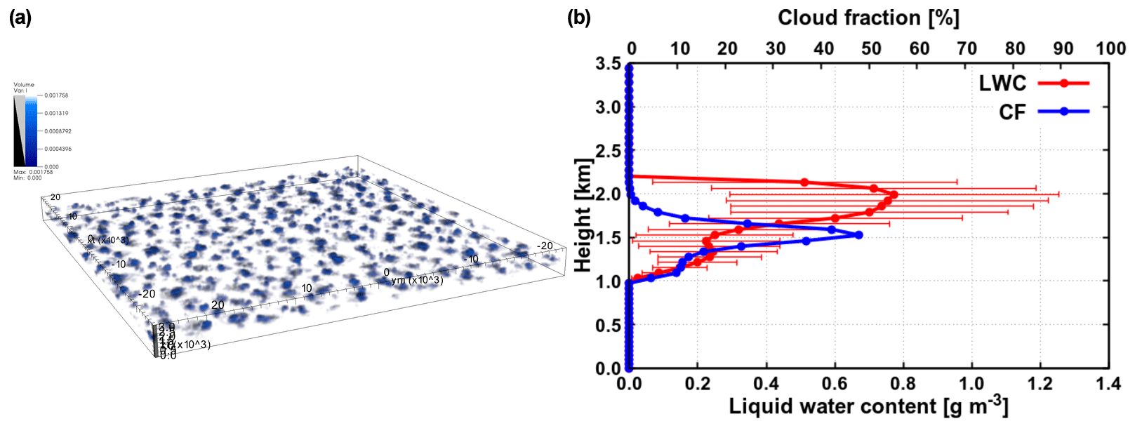
Figure 2 (a) Shallow cumulus cloud field used as input for radiative transfer calculations (visualization with VisIt; Childs et al., 2012). (b) Averaged LWC, its standard deviation (marked with error bars) and cloud fraction.

Figure 3 Horizontal heterogeneity for shallow cumulus cloud field. (a) Cloud mask (clouds in white; clear sky in black). (b) Vertically integrated cloud optical thickness in the visible spectral range, highlighting solely optically thicker convective cores.

2.1.2 Shallow cumulus cloud field case study

Input for radiative transfer calculations is a shallow cumulus cloud field with a total cloud cover of 54.8 % (visualized in Fig. 2), simulated with the University of California, Los Angeles, large-eddy simulation (UCLA-LES) model (Stevens et al., 2005; Stevens, 2007). The horizontal domain size is 51.2×51.2 km², with the vertical extent of the domain being 3.5 km. A constant horizontal grid spacing of 100 m is applied, whereas the vertical grid spacing is variable ranging from 50 m at the ground to 84 m at domain top. Further details about the UCLA-LES setup can be found in Jakub and Mayer (2017). A 3-D LWC distribution was extracted from a simulation snapshot (with a threshold of 10⁻³ g m⁻³) and the corresponding effective radius (R_e) was parameterized according to Bugliaro et al. (2011). Vertical profiles of averaged LWC, its standard deviation (σ_LWC; simplest measure of cloud horizontal inhomogeneity) and cloud fraction are shown in Fig. 2b. Figure 3 shows the cloud mask as well as vertically integrated cloud optical thickness, demonstrating that optically thicker regions are located in the interior of individual clouds, which conforms to the core–shell model.

2.2 Radiative transfer models and experimental setup

2.2.1 Radiative transfer models

The radiative transfer experiments were performed using the libRadtran software (http://www.libradtran.org, 10 July 2020), which contains several radiation solvers. The benchmark calculations were performed with the 3-D model MYSTIC, the Monte Carlo code for the physically correct tracing of photons in cloudy atmospheres (Mayer, 2009), which can be run in ICA mode as well. Further, we employed the classic δ-Eddington two-stream method (Zdunkowski et al., 2007) suitable for horizontally homogeneous layers (either fully cloudy or fully clear sky) and the extension of this method, which allows for partial cloudiness. The latter is the δ-Eddington two-stream method with maximum-random overlap assumption, which was recently implemented in libRadtran in the configuration as described in Črnivec and Mayer (2019) and is ideally suited as a proxy for the conventional GCM radiation scheme.

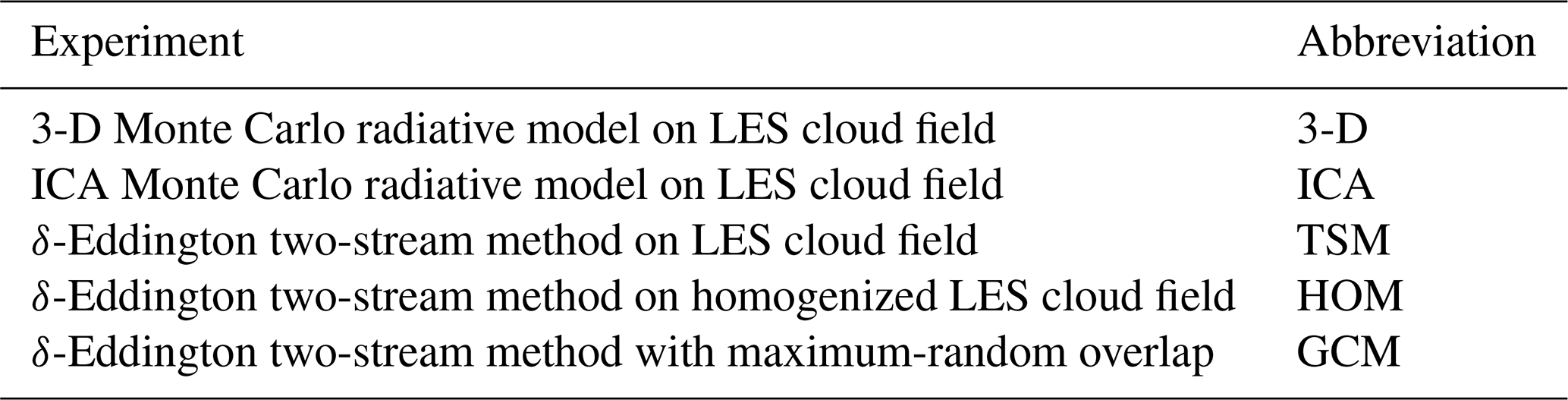
Table 1 List of preliminary radiative transfer experiments and their abbreviations.

2.2.2 Setup of radiative transfer experiments

The background thermodynamic state was the US standard atmosphere (Anderson et al., 1986). The parameterization of Hu and Stamnes (1993) was used to convert LWC and R_e into cloud optical properties. The solar experiments were performed for solar zenith angles (SZAs) of 0, 30 and 60^∘ and a surface albedo of 0.25. In the thermal part of the spectrum, the surface was assumed to be nonreflective. The shortwave calculations applied 32 spectral bands of the correlated-k distribution by Kato et al. (1999), whereas the longwave calculations employed 12 spectral bands adopted from Fu and Liou (1992). In the Monte Carlo experiments, the standard forward and the efficient backward photon tracing were employed in the solar and thermal spectral range respectively. The resulting Monte Carlo noise of domain-averaged quantities is negligible (less than 0.1 %).

2.2.3 Diagnostics and error calculation

The radiative diagnostics include atmospheric heating rate and net (difference between downward and upward) surface flux. Each diagnostic was examined in the solar, thermal (nighttime effect) and total (daytime effect) spectral range. The error is given by the absolute bias (Eq. 1), relative bias (Eq. 2) and for the atmospheric heating rate additionally by the root mean square error evaluated throughout the vertical extent of the cloud layer (Eq. 3):

$$\begin{array}{}\text{(1)}& {\displaystyle }\text{absolute bias}=y-x,\text{(2)}& {\displaystyle }\text{relative bias}=({\displaystyle \frac{y}{x}}-\mathrm{1})\cdot \mathrm{100}\mathit{\%},\text{(3)}& {\displaystyle }\text{cloud-layer RMSE}=\sqrt{\stackrel{\mathrm{‾}}{(y-x{)}^{\mathrm{2}}}},\end{array}$$

where y represents the biased quantity and x represents the benchmark.

2.3 Preliminary radiative transfer experiments

We present a set of preliminary radiative transfer experiments (listed in Table 1), introducing the 3-D benchmark, the ICA and the conventional GCM calculation. Further, we aim to quantify the various error sources of GCM radiative heating rates, in particular the error related to neglected cloud horizontal heterogeneity.

2.3.1 Benchmark heating rate

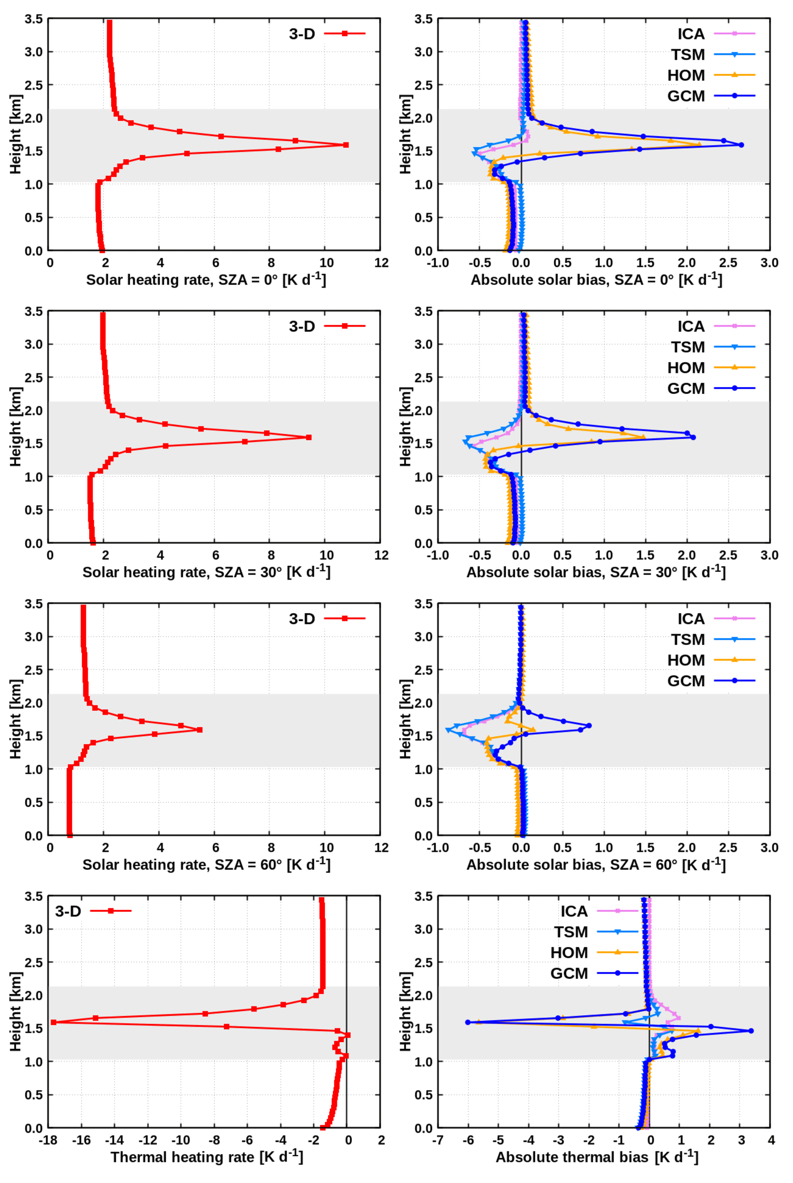
The benchmark calculation using MYSTIC (abbreviated as the “3-D” experiment) was performed on the highly resolved LES cloud field (Fig. 4a). Supposing that the entire LES domain is contained within one GCM column, the quantity of interest is a single vertical profile of radiative heating rate; thus, results were horizontally averaged across the domain. Figure 5 (left) shows the resulting benchmark profiles.

In the solar experiment for overhead Sun (Fig. 5, top left), there is a large absorption of radiation in the cloud layer, resulting in a peak heating rate of 10.8 K d⁻¹. The latter is reached at a height of 1.6 km, which is slightly above the height of maximal cloud fraction (Fig. 2b). With decreasing Sun elevation, the solar heating rate diminishes, exhibiting the maximum of 9.4 and 5.5 K d⁻¹ at SZAs of 30 and 60^∘, respectively. The height where the peak heating is reached stays the same at all SZAs. In the thermal spectral range (Fig. 5, bottom left), the cloud layer is subjected to strong cooling, reaching a peak value of 17.7 K d⁻¹ attained at the same height as the maximum solar heating. Below this height, the magnitude of cooling decreases towards the cloud base, where a slight warming effect is observed.

2.3.2 Conventional GCM representation

In order to mimic the conditions in conventional GCM models (Fig. 4c), the cloud optical properties in each vertical layer were horizontally averaged over the cloudy part of the domain, creating a suite of plane-parallel partially cloudy layers. Consequently, the δ-Eddington two-stream method with maximum-random overlap assumption was employed (abbreviated as the “GCM” experiment).

The main shortcomings of the GCM compared to the benchmark (Fig. 5, right) are as follows. In the solar spectral range, the peak heating rate is overestimated by 2.7, 2.1 and 0.8 K d⁻¹ at SZAs of 0, 30 and 60^∘, respectively. In the thermal spectral range, the GCM bias artificially enhances radiatively driven destabilization of the cloud layer by an overestimation of cooling by 6.0 K d⁻¹ at cloud-layer top and an overestimation of warming by 3.4 K d⁻¹ at cloud-layer bottom. The GCM error sources are multiple: the misrepresentation of realistic cloud structure, the neglected subgrid horizontal photon transport as well as the intrinsic difference between the Monte Carlo and two-stream radiative solvers.

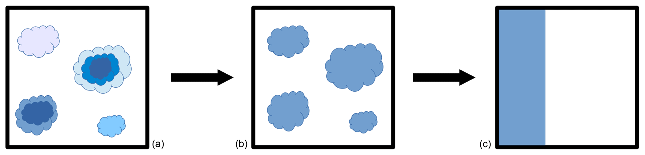
Figure 4 (a) A horizontal cross section of LES cloud field. (b) Derived “homogenized” cloud field, which retains its 3-D geometry but where horizontal heterogeneity is completely removed by applying averaged cloud optical properties in each vertical layer. (c) Conditions in a grid box of a conventional GCM (homogeneous fractional cloudiness).

Figure 5 Radiative heating rate in preliminary experiments. The cloud layer is shaded grey.

2.3.3 ICA and its limitations

To quantify the effect of neglected horizontal photon transport, we run the Monte Carlo radiative model in independent column mode on the original cloud field preserving its LES resolution (Fig. 4a), with the result horizontally averaged over the domain (abbreviated as the “ICA” experiment). Similarly, we applied the δ-Eddington two-stream method within each independent column of the original LES grid (Fig. 4a) and subsequently averaged the result horizontally (abbreviated as the “TSM” experiment). The difference between the ICA and 3-D is a measure of horizontal photon transport. The difference between the TSM and 3-D is a measure of both the horizontal photon transport as well as the intrinsic difference between the Monte Carlo and two-stream radiative solvers.

As anticipated, both independent column experiments (ICA, TSM) perform similarly (Fig. 5, right), implying that the intrinsic difference between the radiative solvers is small. Therefore, only the ICA is discussed hereafter. The solar bias increases with descending Sun (cloud side illumination; Hogan and Shonk, 2013; Jakub and Mayer, 2015, 2016), reaching a maximum of −0.7 K d⁻¹ at an SZA of 60^∘. The amount of thermal cooling is underestimated in the ICA (up to 1 K d⁻¹), since realistic cloud side cooling is neglected (Kablick et al., 2011; Klinger and Mayer, 2014, 2016). Nevertheless, the ICA still overall performs considerably better than the conventional GCM, implying that the major error source of GCM heating rate stems from the misrepresentation of cloud structure and not from the neglected horizontal photon transport.

2.3.4 Cloud horizontal heterogeneity effect

In order to isolate the effects of neglected cloud horizontal heterogeneity in a conventional GCM from other effects related to the misrepresentation of cloud structure (e.g., vertical overlap assumption), we employed the GCM radiative solver on the cloud field preserving its LES resolution but with removed horizontal heterogeneity (Fig. 4b). In this way, the averaged (plane-parallel) cloud optical properties were applied in each vertical layer, but the realistic 3-D cloud field geometry was retained. The results were horizontally averaged (abbreviated as the “HOM” experiment).

The radiative heating rate in the HOM experiment (Fig. 5, right) is to a great extent similar to that in the GCM (especially in the solar experiments at SZAs of 0 and 30^∘, as well as in the thermal experiment), implying that the dominant GCM error source is indeed the neglected cloud horizontal heterogeneity. The question that we attempt to answer is how much of this bias can be removed with Tripleclouds. In other words, how well can the continuous probability density function (PDF) of layer LWC be represented by just two cloudy regions (a two-point PDF)?

3 The Tripleclouds radiative solver

The underlying δ-Eddington two-stream framework employed in the present Tripleclouds implementation differs from that applied by SH08 and subsequent studies (e.g., Shonk et al., 2010; Hogan et al., 2019), whereby the latter is based on the adding method (Lacis and Hansen, 1974) as originally included in the Edwards and Slingo (1996) radiation scheme. Therefore, we first present the δ-Eddington two-stream method (Zdunkowski et al., 2007), already previously contained in libRadtran, and introduce the terminology in Sect. 3.1. We focus only on those aspects of the method, important to understand its extension to multiple (three) regions, explained in subsequent Sect. 3.2. The novel overlap formulation based on the core–shell model is established in Sect. 3.3. Further technical instructions regarding Tripleclouds usage within the scope of libRadtran are provided in Appendix A.

3.1 δ-Eddington two-stream method

In the classic two-stream approach, the entire radiative field is approximated solely with direct solar beam (S) and two streams of diffuse radiation: the downward (E_↓) and upward (E_↑) component. The widely employed δ-Eddington approximation is a reliable way to account for a strong forward-scattering peak of cloud droplets (Joseph et al., 1976; King and Harshvardhan, 1986; Stephens et al., 2001). For the calculations in a vertically inhomogeneous atmosphere, the atmosphere is divided into a number of homogeneous layers, each characterized by its set of constant optical properties. Considering a single layer (j) located between levels (i−1) and (i) (illustrated in Fig. 6)¹, a system of linear equations determining the fluxes emanating from the layer as a function of fluxes entering the layer can be written as

$$\begin{array}{}\text{(4)}& \left(\begin{array}{c}{E}_{\uparrow }(i-\mathrm{1})\\ E_{\downarrow }\left(i\right)\\ S\left(i\right)\end{array}\right)=\left(\begin{array}{ccc}{a}_{\mathrm{11}}& a_{\mathrm{12}}& a_{\mathrm{13}}\\ a_{\mathrm{12}}& a_{\mathrm{11}}& a_{\mathrm{23}}\\ \mathrm{0}& \mathrm{0}& a_{\mathrm{33}}\end{array}\right)\cdot \left(\begin{array}{c}{E}_{\uparrow }\left(i\right)\\ E_{\downarrow }(i-\mathrm{1})\\ S(i-\mathrm{1})\end{array}\right).\end{array}$$

The coefficients a_kl in Eq. (4) are referred to as Eddington coefficients. They depend on the optical properties of layer (j) and have the following physical meaning:

• a₁₁ – transmission coefficient for diffuse radiation,

• a₁₂ – reflection coefficient for diffuse radiation,

• a₁₃ – reflection coefficient for the primary scattered solar radiation,

• a₂₃ – transmission coefficient for the primary scattered solar radiation and

• a₃₃ – transmission coefficient for the direct solar radiation.

The preceding formulation considered solar radiative transfer in the absence of thermal emission. As solar and thermal spectra are separated and can be therefore conveniently treated independently, the solar source is merely replaced with the terrestrial emission term when addressing thermal radiation. The vertical temperature variation is thereby taken into account by allowing the Planck function to vary in accordance with the Eddington-type linearization: $B_{\mathrm{Planck}}\left(\mathit{\tau }\right)=B_{\mathrm{0}}+B_{\mathrm{1}}\mathit{\tau }$, where B₀ and B₁ are constants. The equation system for a single layer is constructed in a similar manner, accounting for both upward and downward thermal emission contributions. For a more comprehensive explanation, the reader is referred to Zdunkowski et al. (2007), as in the rest of this section we will focus on solar radiation.

The individual layers are coupled vertically by imposing flux continuity at each level. Taking the boundary conditions at TOA (Eq. 5) and at the ground (Eq. 6, with A_g representing ground albedo) into account:

$$\begin{array}{}\text{(5)}& {\displaystyle }{E}_{\downarrow }\left(\mathrm{0}\right)=\mathrm{0},\text{(6)}& {\displaystyle }{E}_{\uparrow }\left(N\right)=A_{\mathrm{g}}\left[S\right(N)+E_{\downarrow }(N\left)\right],\end{array}$$

the radiative fluxes throughout the atmosphere are computed by solving the matrix problem (Coakley and Chylek, 1975; Wiscombe and Grams, 1976; Meador and Weaver, 1980; Ritter and Geleyn, 1992). Henceforth, the calculation of heating rates is straightforward.

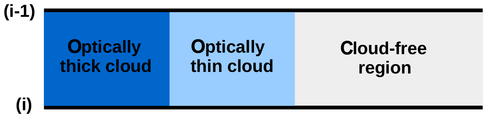
3.2 δ-Eddington two-stream method for three regions at each height

Consider now a model layer located between levels (i−1) and (i) divided into three regions (Fig. 7). Such layer is characterized by three sets of optical properties and corresponding Eddington coefficients: one for the region of optically thick cloud (superscript “ck”), the other for the region of optically thin cloud (superscript “cn”) and the third for the cloud-free region (superscript “f”). In order to apply vertical overlap rules, the radiative fluxes corresponding to each of the three regions need to be defined separately at each level (e.g., S^ck, S^cn and S^f; and analogously for both diffuse components). Total radiative flux at level (i) is thus the sum of both cloudy and the cloud-free components:

$$\begin{array}{}\text{(7)}& {\displaystyle }S\left(i\right)=S^{\mathrm{ck}}\left(i\right)+S^{\mathrm{cn}}\left(i\right)+S^{\mathrm{f}}\left(i\right),\text{(8)}& {\displaystyle }{E}_{\downarrow }\left(i\right)=E_{\downarrow }^{\mathrm{ck}}\left(i\right)+E_{\downarrow }^{\mathrm{cn}}\left(i\right)+E_{\downarrow }^{\mathrm{f}}\left(i\right),\text{(9)}& {\displaystyle }{E}_{\uparrow }\left(i\right)=E_{\uparrow }^{\mathrm{ck}}\left(i\right)+E_{\uparrow }^{\mathrm{cn}}\left(i\right)+E_{\uparrow }^{\mathrm{f}}\left(i\right).\end{array}$$

Equation (4) is replaced by

$$\begin{array}{}\text{(10)}& {\displaystyle }\begin{array}{rl}& \left(\begin{array}{c}{E}_{\uparrow }^{\mathrm{ck}}(i-\mathrm{1})\\ E_{\downarrow }^{\mathrm{ck}}\left(i\right)\\ S^{\mathrm{ck}}\left(i\right)\end{array}\right)=\left(\begin{array}{ccc}{a}_{\mathrm{11}}^{\mathrm{ck}}& a_{\mathrm{12}}^{\mathrm{ck}}& a_{\mathrm{13}}^{\mathrm{ck}}\\ a_{\mathrm{12}}^{\mathrm{ck}}& a_{\mathrm{11}}^{\mathrm{ck}}& a_{\mathrm{23}}^{\mathrm{ck}}\\ \mathrm{0}& \mathrm{0}& a_{\mathrm{33}}^{\mathrm{ck}}\end{array}\right)\\ & \cdot \left(\begin{array}{c}{T}_{\uparrow }^{\mathrm{ck},\mathrm{ck}}{E}_{\uparrow }^{\mathrm{ck}}\left(i\right)+T_{\uparrow }^{\mathrm{cn},\mathrm{ck}}{E}_{\uparrow }^{\mathrm{cn}}\left(i\right)+T_{\uparrow }^{\mathrm{f},\mathrm{ck}}{E}_{\uparrow }^{\mathrm{f}}\left(i\right)\\ T_{\downarrow }^{\mathrm{ck},\mathrm{ck}}{E}_{\downarrow }^{\mathrm{ck}}(i-\mathrm{1})+T_{\downarrow }^{\mathrm{cn},\mathrm{ck}}{E}_{\downarrow }^{\mathrm{cn}}(i-\mathrm{1})+T_{\downarrow }^{\mathrm{f},\mathrm{ck}}{E}_{\downarrow }^{\mathrm{f}}(i-\mathrm{1})\\ T_{\downarrow }^{\mathrm{ck},\mathrm{ck}}{S}^{\mathrm{ck}}(i-\mathrm{1})+T_{\downarrow }^{\mathrm{cn},\mathrm{ck}}{S}^{\mathrm{cn}}(i-\mathrm{1})+T_{\downarrow }^{\mathrm{f},\mathrm{ck}}{S}^{\mathrm{f}}(i-\mathrm{1})\end{array}\right),\end{array}\text{(11)}& {\displaystyle }\begin{array}{rl}& \left(\begin{array}{c}{E}_{\uparrow }^{\mathrm{cn}}(i-\mathrm{1})\\ E_{\downarrow }^{\mathrm{cn}}\left(i\right)\\ S^{\mathrm{cn}}\left(i\right)\end{array}\right)=\left(\begin{array}{ccc}{a}_{\mathrm{11}}^{\mathrm{cn}}& a_{\mathrm{12}}^{\mathrm{cn}}& a_{\mathrm{13}}^{\mathrm{cn}}\\ a_{\mathrm{12}}^{\mathrm{cn}}& a_{\mathrm{11}}^{\mathrm{cn}}& a_{\mathrm{23}}^{\mathrm{cn}}\\ \mathrm{0}& \mathrm{0}& a_{\mathrm{33}}^{\mathrm{cn}}\end{array}\right)\\ & \cdot \left(\begin{array}{c}{T}_{\uparrow }^{\mathrm{ck},\mathrm{cn}}{E}_{\uparrow }^{\mathrm{ck}}\left(i\right)+T_{\uparrow }^{\mathrm{cn},\mathrm{cn}}{E}_{\uparrow }^{\mathrm{cn}}\left(i\right)+T_{\uparrow }^{\mathrm{f},\mathrm{cn}}{E}_{\uparrow }^{\mathrm{f}}\left(i\right)\\ T_{\downarrow }^{\mathrm{ck},\mathrm{cn}}{E}_{\downarrow }^{\mathrm{ck}}(i-\mathrm{1})+T_{\downarrow }^{\mathrm{cn},\mathrm{cn}}{E}_{\downarrow }^{\mathrm{cn}}(i-\mathrm{1})+T_{\downarrow }^{\mathrm{f},\mathrm{cn}}{E}_{\downarrow }^{\mathrm{f}}(i-\mathrm{1})\\ T_{\downarrow }^{\mathrm{ck},\mathrm{cn}}{S}^{\mathrm{ck}}(i-\mathrm{1})+T_{\downarrow }^{\mathrm{cn},\mathrm{cn}}{S}^{\mathrm{cn}}(i-\mathrm{1})+T_{\downarrow }^{\mathrm{f},\mathrm{cn}}{S}^{\mathrm{f}}(i-\mathrm{1})\end{array}\right),\end{array}\text{(12)}& {\displaystyle }\begin{array}{rl}& \left(\begin{array}{c}{E}_{\uparrow }^{\mathrm{f}}(i-\mathrm{1})\\ E_{\downarrow }^{\mathrm{f}}\left(i\right)\\ S^{\mathrm{f}}\left(i\right)\end{array}\right)=\left(\begin{array}{ccc}{a}_{\mathrm{11}}^{\mathrm{f}}& a_{\mathrm{12}}^{\mathrm{f}}& a_{\mathrm{13}}^{\mathrm{f}}\\ a_{\mathrm{12}}^{\mathrm{f}}& a_{\mathrm{11}}^{\mathrm{f}}& a_{\mathrm{23}}^{\mathrm{f}}\\ \mathrm{0}& \mathrm{0}& a_{\mathrm{33}}^{\mathrm{f}}\end{array}\right)\\ & \cdot \left(\begin{array}{c}{T}_{\uparrow }^{\mathrm{ck},\mathrm{f}}{E}_{\uparrow }^{\mathrm{ck}}\left(i\right)+T_{\uparrow }^{\mathrm{cn},\mathrm{f}}{E}_{\uparrow }^{\mathrm{cn}}\left(i\right)+T_{\uparrow }^{\mathrm{f},\mathrm{f}}{E}_{\uparrow }^{\mathrm{f}}\left(i\right)\\ T_{\downarrow }^{\mathrm{ck},\mathrm{f}}{E}_{\downarrow }^{\mathrm{ck}}(i-\mathrm{1})+T_{\downarrow }^{\mathrm{cn},\mathrm{f}}{E}_{\downarrow }^{\mathrm{cn}}(i-\mathrm{1})+T_{\downarrow }^{\mathrm{f},\mathrm{f}}{E}_{\downarrow }^{\mathrm{f}}(i-\mathrm{1})\\ T_{\downarrow }^{\mathrm{ck},\mathrm{f}}{S}^{\mathrm{ck}}(i-\mathrm{1})+T_{\downarrow }^{\mathrm{cn},\mathrm{f}}{S}^{\mathrm{cn}}(i-\mathrm{1})+T_{\downarrow }^{\mathrm{f},\mathrm{f}}{S}^{\mathrm{f}}(i-\mathrm{1})\end{array}\right),\end{array}\end{array}$$

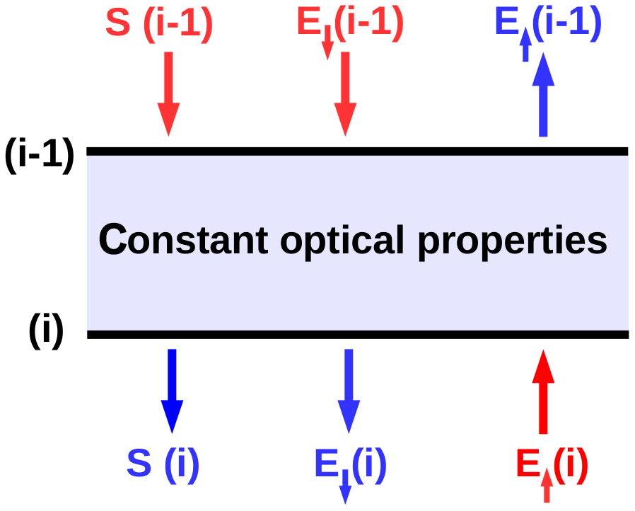
Figure 6 A homogeneous model layer between levels (i−1) and (i). Incoming radiative fluxes are colored red; outgoing fluxes are colored blue.

Figure 7 A model layer between levels (i−1) and (i) divided into three regions.

so that the fluxes emanating from a certain region of the layer under consideration (e.g., region of optically thick cloud) generally depend on a linear combination of the incoming fluxes stemming from each of the three regions in adjacent layers. The coefficients starting with T appearing in Eqs. (10), (11), (12) are referred to as the overlap (transfer) coefficients and correspond to layer (j). The coefficient $T_{\downarrow }^{\mathrm{ck},\mathrm{cn}}\left(j\right)$, for example, represents the fraction of downward radiation that leaves the base of optically thick cloud of layer (j−1) and enters the optically thin cloud of layer under consideration (j). The overlap coefficients quantitatively depend on the choice of the overlap rule, which will be discussed in the next section. For a three-region layer, the boundary condition at TOA (Eq. 5) implies

$$\begin{array}{}\text{(13)}& {\displaystyle }{E}_{\downarrow }^{\mathrm{ck}}\left(\mathrm{0}\right)=\mathrm{0},\text{(14)}& {\displaystyle }{E}_{\downarrow }^{\mathrm{cn}}\left(\mathrm{0}\right)=\mathrm{0},\text{(15)}& {\displaystyle }{E}_{\downarrow }^{\mathrm{f}}\left(\mathrm{0}\right)=\mathrm{0}.\end{array}$$

The boundary condition at the ground (Eq. 6) is extended to

$$\begin{array}{}\text{(16)}& {\displaystyle }{E}_{\uparrow }^{\mathrm{ck}}\left(N\right)=A_{\mathrm{g}}\left[S^{\mathrm{ck}}\right(N)+E_{\downarrow }^{\mathrm{ck}}(N\left)\right],\text{(17)}& {\displaystyle }{E}_{\uparrow }^{\mathrm{cn}}\left(N\right)=A_{\mathrm{g}}\left[S^{\mathrm{cn}}\right(N)+E_{\downarrow }^{\mathrm{cn}}(N\left)\right],\text{(18)}& {\displaystyle }{E}_{\uparrow }^{\mathrm{f}}\left(N\right)=A_{\mathrm{g}}\left[S^{\mathrm{f}}\right(N)+E_{\downarrow }^{\mathrm{f}}(N\left)\right],\end{array}$$

which assumes that the downward fluxes leaving the lowest model layer, after reflection enter the same sections of individual cloudy and cloud-free air (isotropic ground reflection).

3.3 Overlap considerations

The layer cloud fraction C is given by

$$\begin{array}{}\text{(19)}& C\left(j\right)=C^{\mathrm{ck}}\left(j\right)+C^{\mathrm{cn}}\left(j\right).\end{array}$$

In our implementation, we demand the following relationship between the individual cloud fraction components:

$$\begin{array}{}\text{(20)}& {\displaystyle }{C}^{\mathrm{ck}}\left(j\right)=\mathit{\alpha }\cdot C\left(j\right),\text{(21)}& {\displaystyle }{C}^{\mathrm{cn}}\left(j\right)=(\mathrm{1}-\mathit{\alpha })\cdot C\left(j\right),\end{array}$$

where α is a constant between 0 and 1. We apply the widely used maximum-random overlap assumption (Geleyn and Hollingsworth, 1979) for the entire layer cloudiness (sum of optically thick and thin cloudy regions), where adjacent cloudy layers exhibit maximal overlap and cloudy layers separated by at least one cloud-free layer exhibit random overlap. If the cloudy layers are split into two parts, however, this overlap rule is not sufficient and needs to be extended. Therefore, we additionally assume the maximum overlap of optically thicker cloudy regions in pairs of adjacent layers and abbreviate this extended overlap rule to the “maximum²-random overlap”. This assumption implicitly places the optically thicker cloudy region towards the interior of the cloud in the horizontal plane, which is in line with the core–shell model.

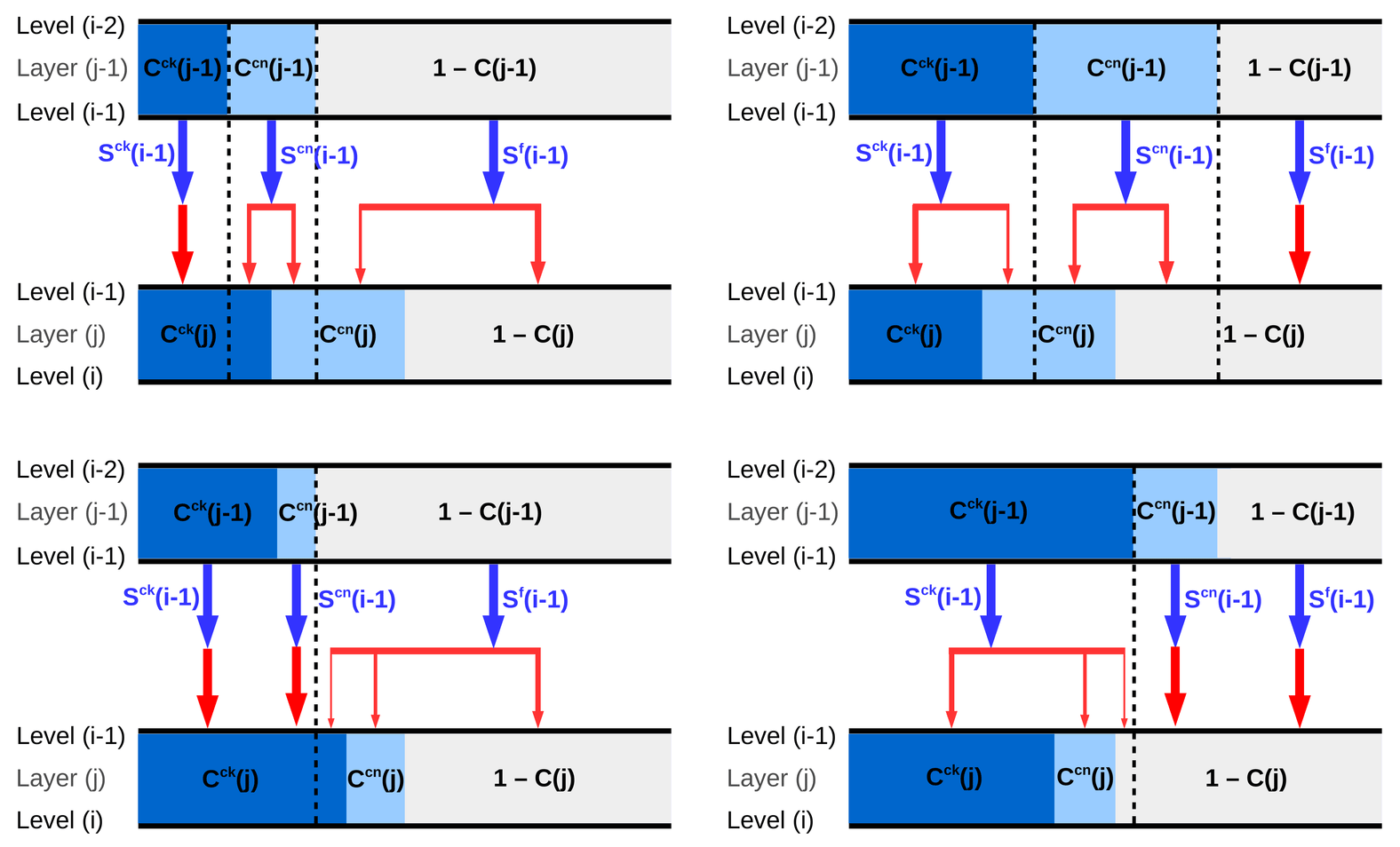
Figure 8 Transmission of direct solar radiation through two adjacent layers with partial cloudiness for the maximum²-random overlap concept.

Now one can quantitatively determine the overlap coefficients in Eqs. (10), (11) and (12) for the maximum²-random overlap. We consider the transmission of downward radiation through two adjacent layers with partial cloudiness. Four possible geometries, illustrated in Fig. 8, need to be treated. For the situation depicted in the top left panel of Fig. 8, the transmission of direct radiation can be formulated as follows. The optically thick cloud of layer (j−1) transmits S^ck(i−1), the optically thin cloud transmits S^cn(i−1) and the cloud-free region transmits S^f(i−1). These three components of the transmitted radiation must then be distributed between the three regions of the lower layer (j). The maximum overlap of optically thick cloudy regions implies that the entire radiation S^ck leaving the base of layer (j−1) enters the optically thick cloud below:

$$\begin{array}{}\text{(22)}& T_{\downarrow }^{\mathrm{ck},\mathrm{ck}}\left(j\right)=\mathrm{1},\end{array}$$

and none of it enters the other two regions:

$$\begin{array}{}\text{(23)}& {\displaystyle }{T}_{\downarrow }^{\mathrm{ck},\mathrm{cn}}\left(j\right)=\mathrm{0},\text{(24)}& {\displaystyle }{T}_{\downarrow }^{\mathrm{ck},\mathrm{f}}\left(j\right)=\mathrm{0}.\end{array}$$

To ensure the maximum overlap of cloudy layers as a whole, the remaining cloudy flux at the base of layer (j−1), namely the S^cn(i−1), needs to be led into the two cloudy regions of the lower layer, with the priority to enter the optically thick cloud. This yields

$$\begin{array}{}\text{(25)}& {\displaystyle }{T}_{\downarrow }^{\mathrm{cn},\mathrm{ck}}\left(j\right)={\displaystyle \frac{C^{\mathrm{ck}}\left(j\right)-C^{\mathrm{ck}}(j-\mathrm{1})}{C^{\mathrm{cn}}(j-\mathrm{1})}},\text{(26)}& {\displaystyle }{T}_{\downarrow }^{\mathrm{cn},\mathrm{cn}}\left(j\right)={\displaystyle \frac{\left[C^{\mathrm{ck}}\right(j-\mathrm{1})-C^{\mathrm{cn}}(j-\mathrm{1}\left)\right]-C^{\mathrm{ck}}\left(j\right)}{C^{\mathrm{cn}}(j-\mathrm{1})}},\text{(27)}& {\displaystyle }{T}_{\downarrow }^{\mathrm{cn},\mathrm{f}}\left(j\right)=\mathrm{0}.\end{array}$$

The cloud-free flux S^f at the base of layer (j−1) is distributed according to

$$\begin{array}{}\text{(28)}& {\displaystyle }{T}_{\downarrow }^{\mathrm{f},\mathrm{f}}\left(j\right)={\displaystyle \frac{\mathrm{1}-C\left(j\right)}{\mathrm{1}-C(j-\mathrm{1})}},\text{(29)}& {\displaystyle }{T}_{\downarrow }^{\mathrm{f},\mathrm{cn}}\left(j\right)={\displaystyle \frac{C\left(j\right)-C(j-\mathrm{1})}{\mathrm{1}-C(j-\mathrm{1})}},\text{(30)}& {\displaystyle }{T}_{\downarrow }^{\mathrm{f},\mathrm{ck}}\left(j\right)=\mathrm{0}.\end{array}$$

The derivation of overlap coefficients for other three geometries involves analogous considerations, whereby the resulting formulas as well as their generalized formulation are given in Appendix B. The transmission of upward radiation is managed via overlap coefficients $T_{\uparrow }^{a,b}\left(j\right)$ in an equivalent manner, except that these are dependent on the cloud fraction in the layer under consideration and that in the layer underneath [C(j), C(j+1)]. It should be noted that the same coefficients govern the reflection, whereby the upward reflection of downward radiation is treated with $T_{\downarrow }^{a,b}$ and the reverse situation is treated with $T_{\uparrow }^{a,b}$. Pairwise overlap as employed here ensures that the matrix problem is fast to solve. Whereas a drawback of the core–shell model and thereby the outlined overlap is that it underperforms in the case of vertically developed cloud systems in strongly sheared conditions, the present Tripleclouds implementation is an excellent tool to study shallow convective clouds. In this way, the effects of cloud horizontal inhomogeneity are tackled in isolation, while the issues related to vertical shear are eliminated.

The Tripleclouds radiative solver has been successfully implemented in the libRadtran package. Technically, the calculation of overlap coefficients is performed in an autonomous function enabling flexible modifications of overlap rules in the future.

4 Methodologies to generate the LWC pair

In order to apply the TC radiative solver, a pair of LWC characterizing optically thin and thick cloudy regions (LWC^cn, LWC^ck) needs to be created in each vertical layer. In Sect. 4.1, we revise the original Tripleclouds method introduced by SH08, later referred to as the “lower percentile method” (Shonk et al., 2010), which can only be applied if the LWC distribution is known. In Sect. 4.2, we summarize the more practical “fractional standard deviation method” (Shonk et al., 2010).

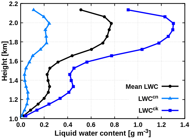
4.1 The lower percentile method

In this method, it is assumed that the LWC distribution in each vertical layer can be approximated with the normal distribution:

$$\begin{array}{}\text{(31)}& p\left(\mathrm{LWC}\right)={\displaystyle \frac{\mathrm{1}}{\sqrt{\mathrm{2}\mathit{\pi }}{\mathit{\sigma }}_{\mathrm{LWC}}}}\exp [-{\displaystyle \frac{(\mathrm{LWC}-\stackrel{\mathrm{‾}}{\mathrm{LWC}}{)}^{\mathrm{2}}}{\mathrm{2}{\mathit{\sigma }}_{\mathrm{LWC}}^{\mathrm{2}}}}],\end{array}$$

where $\stackrel{\mathrm{‾}}{\mathrm{LWC}}$ is layer mean LWC and σ_LWC is its standard deviation. The distribution of LWC is divided into two regions through a given percentile of the distribution, denoted as “split percentile (SP)”. The latter is chosen to be the 50th percentile or the median, which splits the cloud volume into two equal parts (i.e., cloud fraction in each vertical layer is halved). The LWC of the optically thin cloud (LWC^cn) is determined as the value corresponding to the so-called “lower percentile (LP)” of the distribution. This is chosen to be the 16th percentile based on the following considerations. We adjust the two LWC values in a way that the mean LWC in the layer is conserved:

$$\begin{array}{}\text{(32)}& \stackrel{\mathrm{‾}}{\mathrm{LWC}}={\displaystyle \frac{{\mathrm{LWC}}^{\mathrm{ck}}+{\mathrm{LWC}}^{\mathrm{cn}}}{\mathrm{2}}},\end{array}$$

and that they are separated by 2 standard deviations:

$$\begin{array}{}\text{(33)}& {\mathrm{LWC}}^{\mathrm{ck}}-{\mathrm{LWC}}^{\mathrm{cn}}=\mathrm{2}{\mathit{\sigma }}_{\mathrm{LWC}}.\end{array}$$

For a Gaussian distribution, the latter constraint has a desired property that the variability within each of the two cloudy regions (measured by σ_LWC) is the same as that within the entire cloud in the layer. Equations (32) and (33) give the following relationship for LWC^cn:

$$\begin{array}{}\text{(34)}& {\mathrm{LWC}}^{\mathrm{cn}}=\stackrel{\mathrm{‾}}{\mathrm{LWC}}-{\mathit{\sigma }}_{\mathrm{LWC}}.\end{array}$$

The fraction of the distribution with LWC lower than LWC^cn is therefore

$$\begin{array}{}\text{(35)}& f_{\mathrm{cn}}=\underset{-\mathrm{\infty }}{\overset{{\mathrm{LWC}}^{\mathrm{cn}}}{\int }}p\left(\mathrm{LWC}\right)\mathrm{dLWC}=\mathrm{0.159},\end{array}$$

which corresponds to the LP of 16. Finally, the LWC^ck is determined using Eq. (32) to conserve the mean. Figure 9 shows the resulting LWC pair when the LP method is applied on shallow cumulus cloud field.

It should be noted that the choice of the 16th percentile as the LP and the 50th percentile as the SP is based solely on theoretical considerations. In practice, the LP and SP are the two tunable parameters, that can be adjusted according to their performance on real cloud data. Even though the optimal setting varies, SH08 exposed that the combination of LP of 16 and SP of 50 generally serves well in both solar and thermal spectral range for vast ranges of cloud data.

Figure 9 LWC profiles obtained with the LP method.

4.2 Fractional standard deviation method

This method in its initial formulation by Shonk et al. (2010) implicitly assumes that LWC is normally distributed as well. Thereby the cloudiness in each vertical layer is partitioned into two regions of equal size and the pair of LWC (LWC^cn, LWC^ck) is obtained by

$$\begin{array}{}\text{(36)}& {\mathrm{LWC}}^{\mathrm{ck},\mathrm{cn}}=\stackrel{\mathrm{‾}}{\mathrm{LWC}}\pm {\mathit{\sigma }}_{\mathrm{LWC}}=\stackrel{\mathrm{‾}}{\mathrm{LWC}}(\mathrm{1}\pm \mathrm{FSD}),\end{array}$$

where FSD represents the fractional standard deviation of LWC:

$$\begin{array}{}\text{(37)}& \mathrm{FSD}={\displaystyle \frac{{\mathit{\sigma }}_{\mathrm{LWC}}}{\stackrel{\mathrm{‾}}{\mathrm{LWC}}}}.\end{array}$$

Since in practice only $\stackrel{\mathrm{‾}}{\mathrm{LWC}}$ is known within a GCM grid box, the FSD has to be parameterized. A review of numerous studies (Cahalan et al., 1994a; Barker et al., 1996; Pincus et al., 1999; Smith and Del Genio, 2001; Rossow et al., 2002; Hogan and Illingworth, 2003; Oreopoulos and Cahalan, 2005; SH08) carried out by Shonk et al. (2010) gave a globally representative FSD of 0.75±0.18. Figure 10 shows the actual FSD for the present shallow cumulus: although this FSD is strongly dependent on the position within the cloud layer, it predominantly lies within the range of global estimate.

Figure 10 The actual FSD of the shallow cumulus. The grey-shaded area represents the uncertainty of global FSD estimate, centered around its mean value (black line).

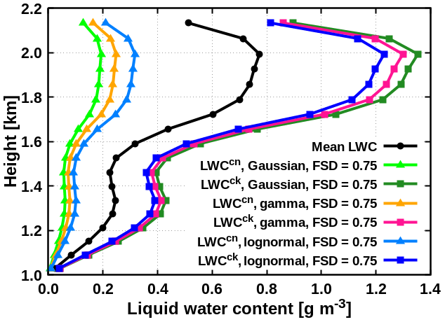
Figure 11 LWC profiles obtained with the FSD method using mean global estimate and altering LWC distribution.

If the cloud condensate is normally distributed, subtracting σ_LWC from the $\stackrel{\mathrm{‾}}{\mathrm{LWC}}$ to obtain the LWC^cn in Eq. (36) corresponds approximately with the 16th percentile. For more realistic lognormal and gamma distributions, the 16th percentile (advocated by SH08) is given by relationships presented in Hogan et al. (2016, 2019), whereby the LWC^ck is again obtained by conserving the layer mean.

In order to test the validity of global FSD estimate, we applied its mean value (0.75) to create the pair of LWC in each vertical layer containing cloud. Further, to test the sensitivity of TC radiative quantities to the assumed form of the subgrid cloud condensate distribution, we employed the FSD method in conjunction with all three distribution assumptions (Gaussian, gamma, lognormal). The resulting LWC profiles are shown in Fig. 11, demonstrating that the LWC pair characterizing the two cloudy regions is clearly sensitive to the distribution assumption, when the mean global FSD estimate is used as a proxy for cloud horizontal inhomogeneity degree.

5 Application

We evaluated the TC radiative solver with both LP and FSD methods. The effective radii characterizing the two cloudy regions were kept the same (averaged R_e). The setup of radiation calculations was as described in Sect. 2.2. The results of the various TC experiments are compared with the conventional GCM, which approximates the cloud condensate distribution with a one-point PDF and can be perceived as an upper bound for the tolerable TC error. In addition, the ICA, which resolves the full subgrid PDF, is shown as well. The atmospheric heating rate is discussed in Sect. 5.1, whereas the net surface flux is investigated in Sect. 5.2.

5.1 Atmospheric heating rate

5.1.1 Tripleclouds with LP method

We assess first the TC radiative solver when the LP method is used to obtain the pair of LWC. The results of this experiment, denoted as “TC(LP)”, are shown in Fig. 12 (middle) and Fig. 13a. It is apparent that the TC(LP) is overall significantly more accurate than the GCM. In the solar spectral range for overhead Sun (Fig. 12, top middle), the maximal bias within the cloud layer is reduced from 2.7 to only 0.7 K d⁻¹. Whereas the largest bias reduction is observed within the cloud layer, the heating rate above and below the cloud layer is considerably improved as well, explained as follows. The non-homogeneous clouds have lower mean shortwave albedo and absorptivity than the corresponding plane-parallel cloudiness with the same mean optical depth (Fig. 2 of Cairns et al., 2000). This implies that the non-homogeneous cloud in the TC configuration reflects less of the incoming solar radiation upward (leading to a reduction of the positive GCM bias above the cloud layer) and simultaneously absorbs less radiation (leading to a reduction of the positive GCM bias in the cloud layer), compared to the homogeneous cloud in the GCM. Consequently, more radiation is transmitted through the cloud layer and absorbed in the region below the cloud layer in the TC experiment compared to that in the GCM, which reduces the negative GCM bias in this region. At an SZA of 30^∘, the behavior is qualitatively similar, with the maximal bias of 2.1 K d⁻¹ within the cloud layer reduced by a factor of 5. At an SZA of 60^∘, the maximal bias of 0.8 K d⁻¹ within the cloud layer becomes of the opposite sign but is still smaller in magnitude (−0.4 K d⁻¹), when the TC(LP) is applied in place of the conventional GCM. In the layer above and especially below the cloud layer, however, the bias is slightly increased. Finally, it should be noted that at low Sun (SZAs of 30 and 60^∘) the TC is generally even more accurate than the ICA, which could be partially due to effective treatment of solar 3-D effects in the TC scheme. It is noteworthy that, at all three SZAs, the 3-D radiation feature at cloud base (increased heating due to surface reflection of radiation) cannot be properly accounted for using the TC solver.

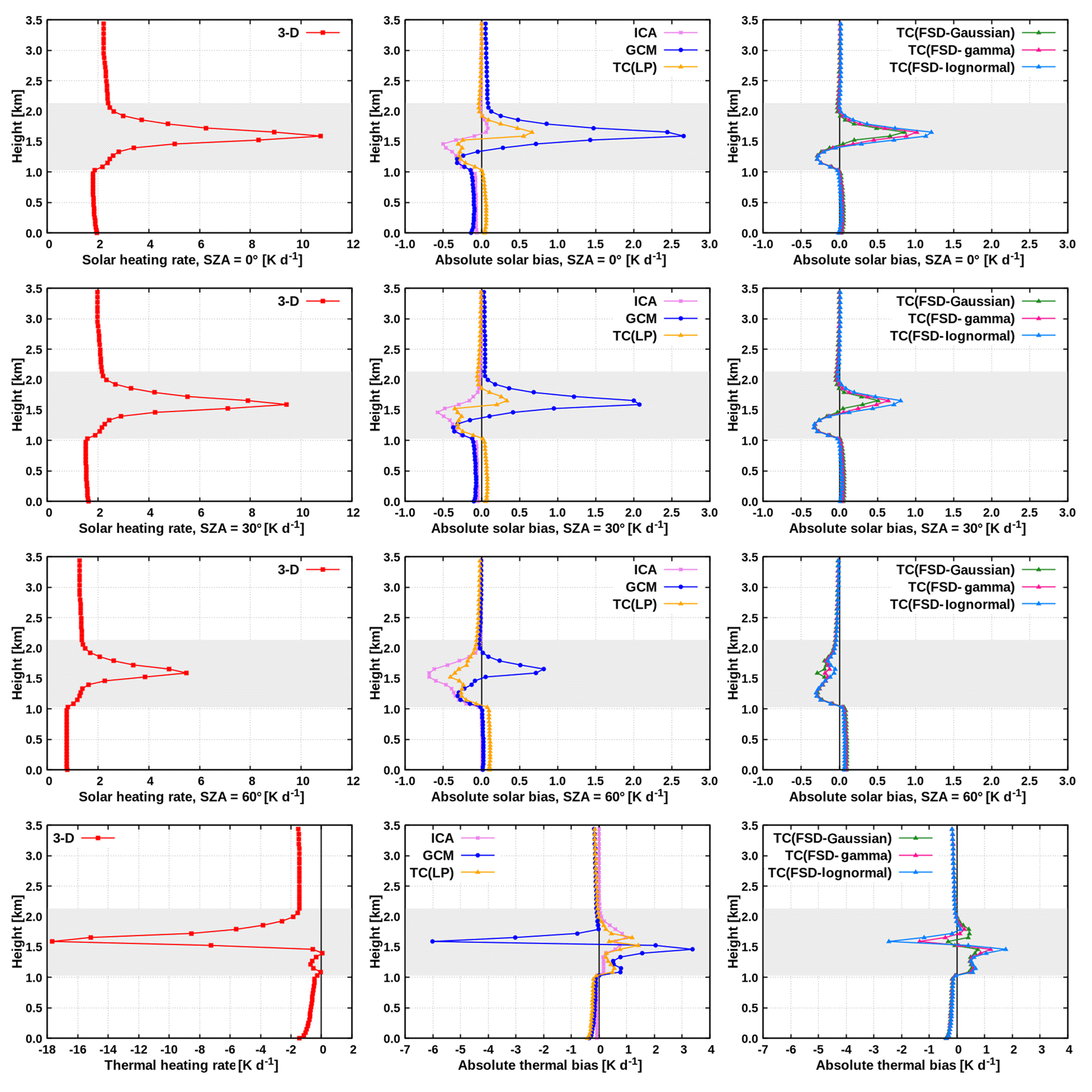
Figure 12 Left: benchmark radiative heating rate. Middle and right: bias for the ICA, GCM and TC experiments.

In the thermal spectral range (Fig. 12, bottom middle), the degree of artificially enhanced destabilization of the cloud layer, arising from the overestimation of cloud-top cooling and cloud base warming in the GCM, is drastically reduced when the TC(LP) is applied, interpreted as follows. The non-homogeneous clouds have lower mean longwave emissivity and absorptivity than the corresponding homogeneous clouds with the same mean optical depth. Thus, the non-homogeneous cloud top in the TC experiment emits less radiation compared to the homogeneous cloud top in the GCM configuration, which reduces the negative GCM bias at cloud top. Similarly, the non-homogeneous cloud base in the TC experiment absorbs less of the radiation stemming from the warmer atmospheric layers underneath the cloud, compared to the homogeneous cloud base in the conventional GCM, which reduces the positive GCM bias at cloud base. As anticipated, in the region above and below the cloud layer, the difference between the TC and the GCM is only marginal. It is noteworthy that the TC performs similarly well to the ICA also in the thermal spectral range, implying that the realistic subgrid cloud variability can be adequately represented by a two-point PDF.

5.1.2 Tripleclouds with FSD method

We investigate now the TC experiments applying the FSD method together with global FSD estimate, shown in Fig. 12 (right) and Fig. 13a. The TC(FSD) experiment assuming the Gaussianity of cloud condensate is examined first – this experiment is considerably more accurate than the conventional GCM as well. As an illustration, the daytime cloud-layer RMSE of 1.7 K d⁻¹ is reduced to 0.3 K d⁻¹ at an SZA of 60^∘ (Fig. 13a). Furthermore, this TC(FSD) experiment is even slightly more accurate than the TC(LP) especially in the thermal spectral range and in the solar spectral range at SZAs of 30 and 60^∘, whereas at an SZA of 0^∘ the situation is reversed (Fig. 12). The largest discrepancy between the two TC experiments is observed in the central part of the cloud layer and is attributed to the fact that the actual layer LWC distribution of the present shallow cumulus deviates from the assumed Gaussian distribution as well as that the actual FSD deviates from the assumed global estimate.

In order to further support these findings, theoretical distributions (see also Appendix C) were fitted to the actual LWC distribution in each vertical cloudy layer (as illustrated in Fig. 14) and the Kolmogorov–Smirnov test (Conover, 1971; Wilks, 1995) was used to assess the goodness of fit. It was found that the actual LWC distribution is best approximated with the gamma distribution (best fit in 55 % of the cloudy layers), followed by the lognormal distribution, whereas the Gaussian distribution always ranked worst. Precisely, the gamma distributional fit performed best throughout the central part of the cloud layer, where cloud–radiative effect is maximized.

Figure 13 (a) RMSE for the ICA, GCM and TC experiments. (b) Comparison of the TC experiments using the FSD method in the baseline setup with global estimate and with the parameterization of Boutle et al. (2014) (denoted as “B”). Note the different scales on the y axis.

When examining the entire set of TC(FSD) experiments with global FSD, it is apparent that the radiative heating rate is considerably more accurate compared to the conventional GCM regardless of the exact assumption for the LWC distribution. Although the Gaussian distribution was ranked worst when fitted to the actual PDF, the Gaussianity assumption with global FSD performed best in practice, contemplated as follows. In the central part of the cloud layer around maximum cloud fraction, the actual FSD of the present shallow cumulus (0.95) is larger than the assumed global estimate. The latter is primarily due to great amount of cloud side area in this region, an essential characteristic of broken cloud field, which generally contributes to increased variability (Boutle et al., 2014; Hill et al., 2012, 2015). Since the assumption of Gaussianity implies the largest difference between the LWC pair characterizing the two cloudy regions (Fig. 11), it partially accounts for the missing variability provided by the global estimate.

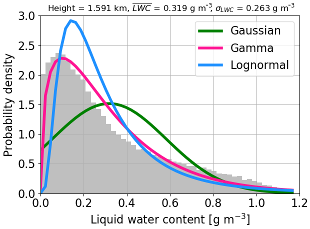
Figure 14 Actual LWC probability density in the central part of the cloud layer and distributional fits.

Based upon these considerations, we additionally evaluated the parameterization of Boutle et al. (2014) for liquid cloud inhomogeneity, which takes into account that variability is cloud fraction dependent. Although solar RMSE slightly reduces when FSD is represented following Boutle et al. (2014), the TC experiment with global FSD constant assuming Gaussian distribution remains the most accurate during both nighttime and daytime (Fig. 13b). To that end, the development of improved parameterizations is highly desired in the future.

Figure 15 (a) benchmark net surface radiative flux. (b, c) bias for the ICA, GCM and TC experiments.

5.2 Net surface flux

Shallow cumulus clouds are a vital part of the planetary boundary layer, where the atmosphere is directly influenced by the presence of the Earth's surface. The net surface radiative flux is the key component of surface energy budget. The radiative biases at the surface, stemming from the inaccurate treatment of clouds, need to be properly understood and possibly best eliminated, as they generally feed back on the biases in the cloudy layers, when the radiation scheme is coupled to a dynamical model.

The behavior of surface biases underneath the present shallow cumulus (Fig. 15b, c) is partially consistent with the findings gained when examining the cloud-layer heating rate error. In the ICA, the daytime net surface flux is underestimated compared to 3-D at all SZAs. This is primarily due to well-acknowledged cloud side escape effect (Várnai and Davies, 1999; Hogan and Shonk, 2013), where the realistic scattering of radiation through cloud side areas increases 3-D downward surface radiation. Even when the Sun is lower in the sky (SZA of 60^∘), this mechanism overcomes the opposing cloud side illumination effect, where an elongated surface shadow reduces the 3-D net surface flux. Similarly, the strength of nocturnal surface cooling is overestimated in the ICA, since realistic cloud side emission is neglected.

The daytime GCM net flux bias at comparatively high Sun (SZAs of 0 and 30^∘) is by a factor of 2 larger than the ICA bias. This is attributed to the fact that the plane-parallel GCM cloudiness leads to an increased solar absorption and hence reduced cloud-layer transmittance. The latter reduces downward flux reaching the surface and profoundly underestimates the net flux. During nighttime, the plane-parallel cloud in the GCM emits a greater amount of radiation towards the surface compared to heterogeneous cloud in the ICA, leading to a reduction of surface net flux bias.

When Tripleclouds is applied – either with the LP or the FSD method utilizing the global estimate – instead of conventional GCM radiation scheme, the daytime net surface flux bias of −55 W m⁻² (or −8 %) is substantially reduced to −5 W m⁻² (or −1 %) at overhead Sun and similarly for an SZA of 30^∘ (assuming Gaussianity of cloud condensate). At an SZA of 60^∘ and especially during nighttime, radiative bias in the various TC experiments increases compared to the GCM bias. Similar findings are obtained if the FSD is parameterized according to Boutle et al. (2014), which does not bring desired improvements (not shown). This indicates that the TC in its current configuration should be taken with caution when applied to surface thermal flux, as its usage can lead to degradation of the nocturnal surface budget compared to simple plane-parallel model.

6 Summary and conclusions

Inspired by the Tripleclouds concept of Shonk and Hogan (2008), we incorporated a second cloudy region in the widely used δ-Eddington two-stream method with maximum-random overlap assumption for partial cloudiness. The resulting radiation scheme thus has one cloud-free and two cloudy regions in each vertical layer and is capable of representing cloud horizontal variability. The inclusion of a second cloudy region into the two-stream framework required an extension of vertical overlap rules. While retaining the maximum-random overlap for the entire layer cloudiness, we additionally assumed the maximum overlap of optically thicker cloudy regions in pairs of adjacent layers. This implicitly places the optically thicker region towards the interior of the cloud in the horizontal plane, while the optically thinner region resides at cloud periphery, which is in line with the core–shell model for convective clouds.

The constructed Tripleclouds radiative solver was evaluated on a shallow cumulus cloud field. The validity of global estimate of fractional standard deviation (a common measure of cloud horizontal variability) as well as of more sophisticated inhomogeneity parameterization was tested along with different assumptions for subgrid cloud condensate distribution (Gaussian, gamma, lognormal), which are frequently applied when representing clouds in weather and climate models. In the vast majority of experiments, Tripleclouds performed better than the conventional plane-parallel GCM scheme. The error of atmospheric heating rate was substantially reduced during daytime and nighttime (up to a 5-fold cloud-layer RMSE reduction). In the event of net surface flux, the daytime bias was generally depleted as well, whereas the nighttime bias was slightly enlarged, suggesting that the computationally more efficient plane-parallel scheme could be retained in this case.

The question that needs to be addressed next is the extent to which our findings for a shallow cumulus case study with intermediate cloud cover apply to a larger set of scenarios comprising a wide range of cloud cover. This question is relevant because horizontal variability might essentially depend on cloud fraction (Boutle et al., 2014; Hill et al., 2012, 2015). Similarly, the degree of cloud horizontal variability depends on the GCM grid resolution (Boutle et al., 2014; Hill et al., 2012, 2015), which has to be investigated in more detail in the future. Furthermore, organizational aspects of shallow convection should be addressed in the context of the present study. Mesoscale shallow convection sometimes occurs in the form of uniformly scattered cumuli but is also frequently organized into cloud streets, clusters or mesoscale arcs (Agee et al., 1973; Atkinson and Zhang, 1996; Wood and Hartmann, 2006; Seifert and Heus, 2013). The classification of rich spatial patterns into various mesoscale cloud morphologies can thereby valuably be performed with deep learning algorithms (e.g., Yuan et al., 2020). The robustness of the present results on the nature of cloud organization should be examined next. Recently, Stevens et al. (2019) proposed four mesoscale cloud patterns frequently observed in trade wind regions, which they labeled “Sugar”, “Flower”, “Fish” and “Gravel”. A follow-up study of Rasp et al. (2019) proved that the four patterns correspond to physically meaningful cloud regimes, each of them being associated with specific large-scale environmental conditions. These climatologically distinct environments should exhibit highly variable cloud water variance. If this proves true and if the internal cloud variability is properly quantified, a regime-dependent fractional standard deviation could be passed into the Tripleclouds radiative solver in the next generation of global models.

An equivalent analysis then needs to be repeated for ice clouds. In order to carry out the analysis for clouds of large vertical growth, such as deep convective clouds, in a strongly sheared environment, the present vertical overlap rules have to be generalized. These topics are currently investigated by the corresponding author of this paper and will be discussed in detail in upcoming studies.

Appendix A: Technical instructions for libRadtran users

The libRadtran radiative package is still under steady, continuous development. The latter goes hand in hand, inter alia, with its plenty satisfied users worldwide. The core of the libRadtran package is the uvspec radiative transfer model, which contains several radiative transfer equation (RTE) solvers. To promote the usage of recently implemented Tripleclouds scheme, which is coded in C programming language, basic guidelines are given below. For a complete description on how to set up the background atmosphere and other input parameters, the reader is referred to the libRadtran user manual, which is included in the software package. The output quantities involve either radiative fluxes (default) (W m⁻²) or heating rates (K d⁻¹). The Tripleclouds radiative solver (termed “twomaxrnd3C”) as described in Sect. 3 of the present work is thus invoked as demonstrated in Fig. A1.

The cloud fraction vertical profile is specified with the standard libRadtran file cf.dat. It is important to note that this file determines the cloud fraction of the entire layer cloudiness (sum of optically thick and thin cloudy regions). The division of the latter into two components is managed via newly introduced parameter twomaxrnd3C_scale_cf, which corresponds to the parameter α in Eqs. (20) and (21). The split of averaged cloud water properties into two components is not yet automated; rather, the user is asked to preprocess both cloud files depending on his/her specific needs. The resulting wck.dat and wcn.dat are 1-D water cloud files, defining properties of optically thick and thin cloudy regions, respectively (note that the option profile_file is solely the generalization of the standard wc_file command). Whereas the provided example illustrates the treatment of water clouds, the solver can be applied to ice clouds in a similar fashion.

Figure A1 An example of invoking the Tripleclouds solver within libRadtran.

Appendix B: Transfer coefficients for the maximum²-random overlap

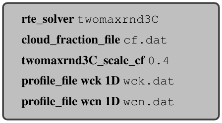
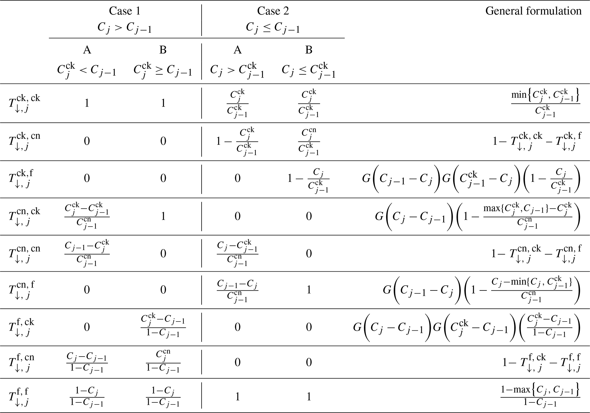
Table B1 contains the transfer (overlap) coefficients for the four cloud geometries depicted in Fig. 8, denoted as case “1-A” (top left panel), “1-B” (bottom left panel), “2-A” (top right panel) and “2-B” (bottom right panel). In order to simplify the handling of various overlap geometries, it is convenient to implement the operator G:

$$G\left(x\right)=\left\{\begin{array}{ll}\mathrm{1},& \text{if }x>\mathrm{0}\\ \mathrm{0},& \text{if }x\le \mathrm{0}.\end{array}\right.$$

Hence, the generalized overlap coefficients can be formulated as exposed in the rightmost column of Table B1.

Table B1 The transfer coefficients $T_{\downarrow }^{a,b}\left(j\right)$ for the four cloud geometric arrangements as well as their general form.

Appendix C: Analytical probability density functions

In the following, we outline the relationship between $\stackrel{\mathrm{‾}}{\mathrm{LWC}}$, the fractional standard deviation of LWC (herein denoted as f_LWC) and the parameters used to describe lognormal and gamma distributions, which were applied to fit the actual LWC distributions.

A lognormal distribution of LWC is defined as

$$\begin{array}{}\text{(C1)}& p\left(\mathrm{LWC}\right)={\displaystyle \frac{\mathrm{1}}{\sqrt{\mathrm{2}\mathit{\pi }}{\mathit{\sigma }}_{\mathrm{0}}\mathrm{LWC}}}\exp [-{\displaystyle \frac{\ln (\mathrm{LWC}/{\mathrm{LWC}}_{\mathrm{0}}{)}^{\mathrm{2}}}{\mathrm{2}{\mathit{\sigma }}_{\mathrm{0}}^{\mathrm{2}}}}].\end{array}$$

The parameters of the lognormal distribution, LWC₀ and σ₀, can be defined in terms of $\stackrel{\mathrm{‾}}{\mathrm{LWC}}$ and f_LWC in the following fashion:

$$\begin{array}{}\text{(C2)}& {\mathrm{LWC}}_{\mathrm{0}}={\displaystyle \frac{\stackrel{\mathrm{‾}}{\mathrm{LWC}}}{\sqrt{f_{\mathrm{LWC}}+\mathrm{1}}}},{\mathit{\sigma }}_{\mathrm{0}}^{\mathrm{2}}=\ln (f_{\mathrm{LWC}}+\mathrm{1}).\end{array}$$

A gamma distribution of LWC is defined as

$$\begin{array}{}\text{(C3)}& p\left(\mathrm{LWC}\right)={\displaystyle \frac{\mathrm{1}}{\mathrm{\Gamma }\left(\mathit{\nu }\right)}}\left({\displaystyle \frac{\mathit{\nu }}{\stackrel{\mathrm{‾}}{\mathrm{LWC}}}}{)}^{\mathit{\nu }}{\mathrm{LWC}}^{\mathit{\nu }-\mathrm{1}}\exp \right[-{\displaystyle \frac{\mathit{\nu }\mathrm{LWC}}{\stackrel{\mathrm{‾}}{\mathrm{LWC}}}}],\end{array}$$

where Γ(ν) denotes the gamma function and the parameter of the distribution ν is related to f_LWC as follows:

$$\begin{array}{}\text{(C4)}& \mathit{\nu }=({\displaystyle \frac{\mathrm{1}}{f_{\mathrm{LWC}}}}{)}^{\mathrm{2}}.\end{array}$$