Measurement report: Statistical modelling of long-term trends of atmospheric inorganic gaseous species within proximity of the pollution hotspot in South Africa

South Africa is considered an important source region of atmospheric pollutants, which is compounded by high population and industrial growth. However, this region is understudied, especially with regard to evaluating long-term trends of atmospheric pollutants. The aim of this study was to perform statistical modelling of SO₂, NO₂ and O₃ long-term trends based on 21-, 19- and 16-year passive sampling datasets available for three South African INDAAF (International Network to study Deposition and Atmospheric Chemistry in Africa) sites located within proximity of the pollution hotspot in the industrialized north-eastern interior in South Africa. The interdependencies between local, regional and global parameters on variances in SO₂, NO₂ and O₃ levels were investigated in the model. Average monthly SO₂ concentrations at Amersfoort (AF), Louis Trichardt (LT) and Skukuza (SK) were 9.91, 1.70 and 2.07 µg m⁻³, respectively, while respective mean monthly NO₂ concentrations at each of these sites were 6.56, 1.46 and 2.54 µg m⁻³. Average monthly O₃ concentrations were 50.77, 58.44 and 43.36 µg m⁻³ at AF, LT and SK, respectively. Long-term temporal trends indicated seasonal and inter-annual variability at all three sites, which could be ascribed to changes in meteorological conditions and/or variances in source contribution. Local, regional and global parameters contributed to SO₂ variability, with total solar irradiation (TSI) being the most significant factor at the regional background site LT. Temperature (T) was the most important factor at SK, located in the Kruger National Park, while population growth (P) made the most substantial contribution at the industrially impacted AF site. Air masses passing over the source region also contributed to SO₂ levels at SK and LT. Local and regional factors made more substantial contributions to modelled NO₂ levels, with P being the most significant factor explaining NO₂ variability at all three sites, while relative humidity (RH) was the most important local and regional meteorological factor. The important contribution of P on modelled SO₂ and NO₂ concentrations was indicative of the impact of increased anthropogenic activities and energy demand in the north-eastern interior of South Africa. Higher SO₂ concentrations, associated with lower temperatures, as well as the negative correlation of NO₂ levels to RH, reflected the influence of pollution build-up and increased household combustion during winter. The El Niño–Southern Oscillation (ENSO) made a significant contribution to modelled O₃ levels at all three sites, while the influence of local and regional meteorological factors was also evident. Trend lines for SO₂ and NO₂ at AF indicated an increase in SO₂ and NO₂ concentrations over the 19-year sampling period, while an upward trend in NO₂ levels at SK signified the influence of growing rural communities. Marginal trends were observed for SO₂ at SK, as well as SO₂ and NO₂ at LT, while O₃ remained relatively constant at all three sites. SO₂ and NO₂ concentrations were higher at AF, while the regional O₃ problem was evident at all three sites.

1 Introduction

Although Africa is regarded as one of the most sensitive continents with regard to air pollution and climate change, it is the least studied (Laakso et al., 2012). South Africa is considered an important source region of atmospheric pollutants within the African continent, which is attributed to its highly industrialized economy with the most significant industrial activities including mining, metallurgical and petrochemical activities, as well as large-scale coal-fired electricity generation (Rorich and Galpin, 1998; Tiitta et al., 2014). Atmospheric pollution associated with South Africa is compounded by high population growth that, in turn, drives further economic and industrial growth leading to an ever-increasing energy demand (Tiitta et al., 2014; World Bank, 2019; International Energy Agency, 2020). The extent of air pollution in South Africa is illustrated by the well-known NO₂ pollution hotspot revealed by satellite data over the Mpumalanga Highveld, where 11 coal-fired power stations are located (Lourens et al., 2011), which was also recently indicated by the newly launched European Space Agency Sentinel-5P satellite (Meth, 2018).

The importance of long-term atmospheric chemical measurements has been indicated by numerous studies on atmosphere–biosphere interactions (Fowler et al., 2009) and air quality (Monks et al., 2009). These long-term assessments are crucial in identifying relevant policy requirements on local and global scales, as well as the most topical atmospheric-chemistry research questions (Vet et al., 2014). In 1990, the International Global Atmospheric Chemistry (IGAC) programme, in collaboration with the Global Atmosphere Watch (GAW) network of the World Meteorological Organization (WMO) initiated the Deposition of Biogeochemically Important Trace Species (DEBITS) project with the aim to conduct long-term assessments of atmospheric biogeochemical species in the tropics – a region for which limited data existed (Lacaux et al., 2003). The programme is currently operated within the framework of the third phase of IGAC and within the context of the International Nitrogen Initiative (INI) programme. The African component of this initiative was historically referred to as IGAC DEBITS Africa (IDAF), which was relabelled in 2015/2016 as the International Network to study Deposition and Atmospheric Chemistry in Africa (INDAAF) programme. The INDAAF long-term network currently consists of 13 monitoring sites, strategically positioned in southern, western and central Africa, which are representative of the most important African ecosystems (http://indaaf.obs-mip.fr, last access: 12 October 2018). Typical measurements at the INDAAF sites include wet-only rain collection, aerosol composition and inorganic gaseous concentrations, determined with passive samplers.

Long-term measurements have been conducted at three dry-savannah southern African INDAAF sites, which include Amersfoort (AF), Louis Trichardt (LT) and Skukuza (SK) located within proximity of the pollution hotspot in the north-eastern interior of South Africa. Measurement of inorganic gaseous pollutant species, i.e. sulfur dioxide (SO₂), nitrogen dioxide (NO₂) and ozone (O₃), has been conducted since 1995 at LT, 1997 at AF and 2000 at SK utilizing passive samplers. These gaseous species are generally associated with the above-mentioned major sources of atmospheric pollutants in South Africa (Connell, 2005). Moreover, a large number of these sources are located within the north-eastern interior of South Africa and include the Mpumalanga Highveld, the Johannesburg–Pretoria conurbation and the Vaal Triangle. Laban et al. (2018), for instance, recently indicated high O₃ levels in this north-eastern interior of South Africa, while it was also indicated that O₃ formation in this region can be considered NO_x-limited due to high NO₂ concentrations. Therefore, the South African INDAAF sites were strategically positioned to be representative of the South African interior, with AF being an industrially influenced site, LT being a rural background site and SK being a background site located in the Kruger National Park, as indicated in Fig. 1.

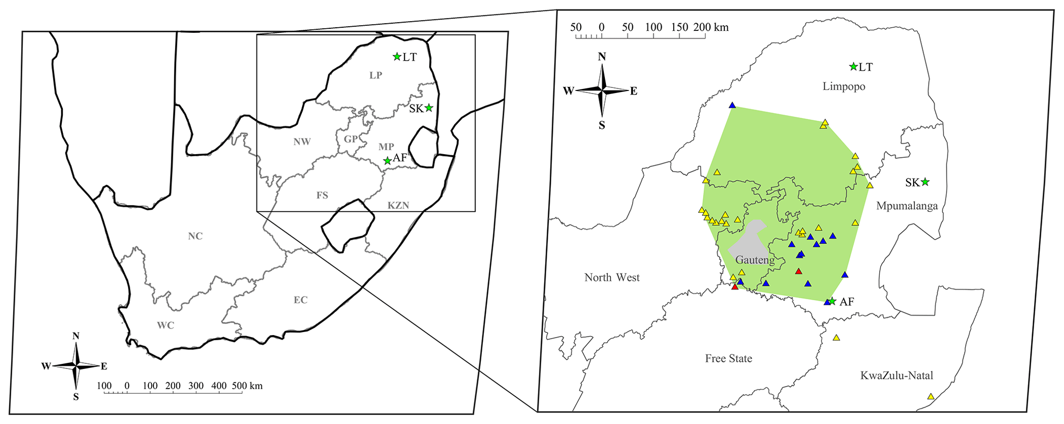
Figure 1 Regional map of South Africa indicating the measurement sites at Amersfoort (AF), Louis Trichardt (LT) and Skukuza (SK) with green stars. A zoomed-in map indicates the defined source region, the Johannesburg–Pretoria conurbation (grey polygon) and large point sources, i.e. power stations (blue triangles), petrochemical plants (red triangles) and pyrometallurgical smelters (yellow triangles).

A number of studies have been reported on measurements conducted within the INDAAF network (Martins et al., 2007; Adon et al., 2010, 2013; Josipovic et al., 2011), presenting inorganic gaseous concentrations at southern, as well as western and central, African sites, respectively. Conradie et al. (2016) recently reported on precipitation chemistry at the South African INDAAF sites, while Maritz et al. (2019) conducted an assessment of particulate organic and elemental carbon at these sites. However, in-depth analysis of long-term trends of atmospheric pollutants at the INDAAF sites has not been conducted due to the non-availability of long-term data. Therefore, the aim of this study was to perform statistical modelling of SO₂, NO₂ and O₃ long-term trends based on 21-, 19- and 16-year datasets available for LT, AF and SK, respectively. The influences of sources together with local, regional and global meteorological patterns on the atmospheric concentrations of SO₂, NO₂ and O₃ were considered in the model.

2 Measurement site and experimental methods

2.1 Site description

Detailed site descriptions have been presented in the literature, e.g. Mphepya et al. (2004, 2006) and Conradie et al. (2016). AF (1628 m above mean sea level, a.m.s.l.) and LT (1300 m a.m.s.l.) are located within the South African Highveld, while SK is situated in the South African Lowveld. As indicated in Fig. 1, AF is in close proximity to the major industrial activities in the Mpumalanga Highveld (∼50 to 100 km north-west) and ∼ 200 km east of the Johannesburg–Pretoria conurbation. LT is located in a rural region mainly associated with agricultural activity, while SK (267 m a.m.s.l) is situated in the Kruger National Park, i.e. natural bushveld in a protected area.

A summary of the regional meteorology of the South African interior, especially relating to the north-eastern part, was presented by Laakso et al. (2012) and Conradie et al. (2016). Meteorology in the South African interior exhibits strong seasonal variability. This region is characterized by anticyclonic air mass circulation, which is especially predominant during winter, resulting in pronounced inversion layers trapping pollutants near the surface (Tyson et al., 1996; Garstang et al., 1996; Gierens et al., 2019). In addition, the north-eastern interior (as most parts of the South African interior) is also characterized by distinct wet and dry seasons, with the wet season occurring typically from mid-spring up to autumn (mid-October to mid-May) (Hewitson and Crane, 2006; Conradie et al., 2016).

In Fig. 2, the air mass history for LT, AF and SK for the entire sampling periods at each site is presented by means of overlaid back trajectories; 96 h back trajectories arriving hourly at each site at a height of 100 m were calculated with the Hybrid Single Particle Lagrangian Integrated Trajectory (HYSPLIT) model (version 4.8), developed by the National Oceanic and Atmospheric Administration (NOAA) Air Resources Laboratory (ARL) (Draxler and Hess, 2014).

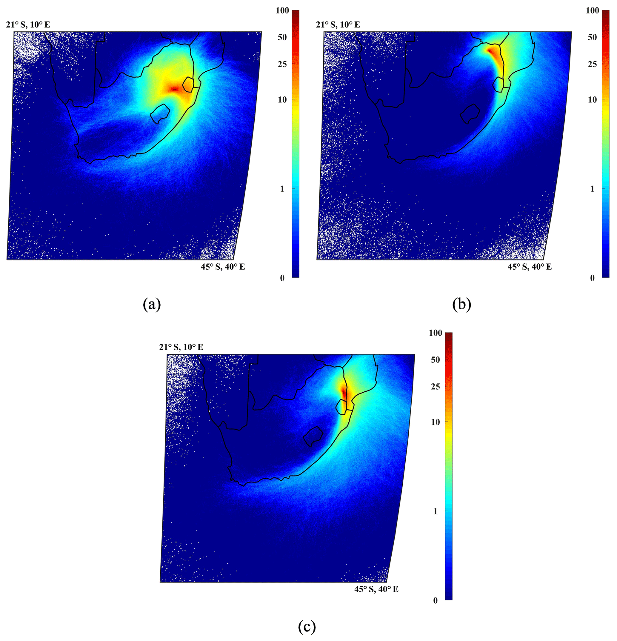
Figure 2 Overlaid hourly arriving 96 h back trajectories for air masses arriving at (a) AF from 1997 to 2015, (b) LT from 1995 to 2015 and (c) SK from 2000 to 2015.

Meteorological data were obtained from the Global Data Assimilation System (GDAS) archive of the National Centers for Environmental Prediction (NCEP) of the United States National Weather Service. Back trajectories were overlaid with fit-for-purpose programming software on a map area divided into grid cells of 0.2^∘ × 0.2^∘. A colour scale presents the frequency of back trajectories passing over each grid cell, with dark blue indicating the lowest and dark red the highest percentage. The predominant anticyclonic air mass circulation over the interior of South Africa is reflected by the overlay back trajectories at each site, while it also indicates that AF is frequently impacted by air masses passing over the major sources in the north-eastern interior. In addition, it is also evident that the rural background sites (LT and SK) are also impacted by the regional circulation of air masses passing over the major sources.

2.2 Sampling, analysis and data quality

Passively derived SO₂, NO₂ and O₃ concentrations were available from 1995 to 2015, 1997 to 2015 and 2000 to 2015 for LT, AF and SK, respectively. Gaseous SO₂, NO₂ and O₃ concentrations were measured utilizing passive samplers manufactured at the North-West University, which are based on the Ferm (1991) passive sampler. Detailed descriptions on the theory and functioning of these passive samplers, which are based on laminar diffusion and chemical reaction of the atmospheric pollutant of interest, have been presented in the literature (Ferm, 1991; Dhammapala, 1996; Martins et al., 2007; Adon et al., 2010). In addition, the passive samplers utilized in this study have been substantiated through a number of inter-comparison studies (Martins et al., 2007; He and Bala, 2008).

Samplers were exposed in duplicate sets for each gaseous species at each measurement site (1.5 m above ground level) for a period of approximately 1 month and returned to the laboratory for analysis. Blank samples were kept sealed in the containers for each set of exposed samplers. Prior to 2008, SO₂ and O₃ passive samples were analysed with a Dionex 100 Ion Chromatograph (IC), while NO₂ samples were analysed with a Cary 50 ultraviolet–visible (UV/Vis) spectrometer up until 2012. SO₂ and O₃ samples collected after 2008, and NO₂ samples collected after 2012, were analysed with a Dionex ICS-3000 system. Data quality of the analytical facilities is ensured through participation in the World Meteorological Organization (WMO) bi-annual Laboratory Intercomparison Study (LIS). The results of the 50th LIS study in 2014 indicated that the recovery of each ion in standard samples was between 95 % and 105 % (Conradie et al., 2016). Analysed data were also subjected to the Q test, with a 95 % confidence threshold to identify, evaluate and reject outliers in the datasets.

2.3 Multiple linear regression model

Similar to the approach employed by Swartz et al. (2020) for the Cape Point GAW station, a multiple linear regression (MLR) model was utilized to statistically evaluate the influence of sources and meteorology on the concentrations of SO₂, NO₂ and O₃ at AF, LT and SK. This model was also utilized by Toihir et al. (2018) and Bencherif et al. (2006) for trend estimates of O₃ and temperature, respectively. MLR analysis models the relationship between two or more independent variables and a dependent variable by fitting a linear equation to the observed data, which can be utilized to calculate values for the dependent variable. In this study, concentrations of inorganic gaseous species (SO₂, NO₂ and O₃) were considered the dependent variable (C(t)), while local, regional and global factors were considered independent variables to yield the following general equation:

$$\begin{array}{}\text{(1)}& C\left(t\right)=\sum _{k=\mathrm{1}}^{p}a\left(k\right)\times f\left(t,k\right)+R^{\prime }\left(t\right),\end{array}$$

where f(t,k) describes the specific factor k at time t; a(k) is the coefficient calculated by the model for the factor k that minimizes the root mean square error (RMSE); and R^′(t) is the residual term that accounts for factors that may have an influence on the model, which are not considered in the MLR model. The RMSE compares the calculated values with the measured values as follows:

$$\begin{array}{}\text{(2)}& {\mathit{\chi }}^{\mathrm{2}}={\left[\sum _{t}C\left(t\right)-\sum _{k}a\left(k\right)\times f(t,k)\right]}^{\mathrm{2}}.\end{array}$$

The trend was parameterized as linear: trend $\left(t\right)={\mathit{\alpha }}_{\mathrm{0}}+{\mathit{\alpha }}_{\mathrm{1}}\cdot t$, where t denotes the time range, α₀ is a constant, α₁ is the slope of the trend (t) line that estimates the trend over the timescale.

The significance of each of the independent variables on the calculated C(t) was evaluated by the relative-importance weight (RIW) approach, which examines the relative contribution that each independent variable makes to the dependent variable and ranks independent variables in order of significance (Nathans et al., 2012; Kleynhans et al., 2017). The RIW approach was applied with IBM^® SPSS^® Statistics version 23, together with programme syntaxes and scripts adapted from Kraha et al. (2012) and Lorenzo-Seva et al. (2010).

2.4 Input data

Global meteorological factors considered in the model included total solar irradiation (TSI), the El Niño–Southern Oscillation (ENSO), the Indian Ocean Dipole (IOD), the quasi-biennial oscillation (QBO) and the Southern Annular Mode (SAM). Data for the ENSO and QBO cycles were obtained from the National Oceanic and Atmospheric Administration (NOAA) (NOAA, 2015a, b), while TSI and IOD data were obtained from the Royal Netherlands Meteorological Institute (Koninklijk Nederlands Meteorologisch Instituut) (KMNI, 2016a, b). SAM data were obtained from the National Environmental Research Council's British Antarctic Survey (Marshall, 2018). The initial input parameters for the model only included the global force factors in order to assess the importance of individual global predictors on measured gaseous concentrations.

Local and regional meteorological parameters included in the model were rain depth (R), relative humidity (RH) and ambient temperature (T), as well as monthly averaged wind direction (W_d) and wind speed (W_s). Since meteorological parameters were not measured at the three sites during the entire sampling period, meteorological data were obtained from the European Centre for Medium-Range Weather Forecasts (ECMWF) reanalysis interim archive (ERA). Although meteorological measurements were conducted by the South African Weather Service within relative proximity of the locations of the three sites, the data coverage for all the meteorological parameters for the entire sampling period was relatively low (<50 %). Planetary boundary layer (PBL) heights were obtained from the global weather forecast model operated by the ECMWF (Korhonen et al., 2014). Population data (P) from three separate national censuses were obtained from local municipalities and were also included in the model.

Daily fire distribution data from 2000 to 2015 were derived from the National Aeronautics and Space Administration's (NASA) Moderate Resolution Imaging Spectrometer (MODIS) satellite retrievals. MODIS is mounted on the polar-orbiting Earth Observation System's (EOS) Terra spacecraft and globally measures, among others, burn scars, fire and smoke distributions. This dataset was retrieved from the NASA Distributed Active Archive Centers (DAACs) (Kaufman et al., 2003). Fire events were separated into the categories of a local fire event (LFE), occurring within a 100 km radius from a respective site, and a regional fire event (DFE), taking place between 100 and 1000 km from each site.

Hourly arriving back trajectories (as discussed above) were also used to calculate the percentage time that air masses spent over a predefined source region (Fig. 1) before arriving at each of the sites for each month, which was also a parameter (source region; SR) included in the statistical model. The source region is a combination of source regions defined in previous studies, e.g. Jaars et al. (2014) and Booyens et al. (2019), which comprised the Mpumalanga Highveld, Vaal Triangle, the Johannesburg–Pretoria conurbation, the western and the eastern Bushveld Igneous Complex (Fig. 1).

Since data were not available for certain local and regional factors considered in the model for the entire sampling periods at AF, LT and SK and in an effort to include the optimum number of local and regional factors available for each site, modelled concentrations could not be calculated for the entire sampling periods when global, regional and local factors were included in the MLR model.

3 Results

Figures A1, A2 and A3 in Appendix A present the time series of monthly average SO₂, NO₂ and O₃ concentrations measured at AF (1997–2015), LT (1995–2015) and SK (2000–2015). Seasonal and inter-annual variability associated with changes in the prevailing meteorology and source contributions will be evaluated and statistically assessed using a multiple linear regression model in subsequent sections.

3.1 Seasonal and inter-annual variability

In Figs. 3, 4 and 5, the monthly SO₂, NO₂ and O₃ concentrations, respectively, at AF, LT and SK, determined for the entire sampling periods, are presented. Monthly variability in concentrations of these species at these three sites is expected. The north-eastern interior of South Africa, where these sites are located, is generally characterized by increased concentrations in pollutant species during the dry winter months (June to September) due to the prevailing meteorological conditions (Conradie et al., 2016). More pronounced inversion layers trap pollutants near the surface, which, in conjunction with increased anticyclonic recirculation and decreased wet deposition, leads to the build-up of pollutant levels (Conradie et al., 2016; Laban et al., 2018). In addition, increased household combustion for space heating during winter also contributes to higher levels of atmospheric pollutants, while open biomass burning (wildfires) is also a significant source of atmospheric species in late winter and spring (August to November). Species typically associated with biomass burning (open or household) include particulate matter (PM), CO and NO₂, while household combustion can also contribute to SO₂ emissions depending on the type of fuel consumed. CO and NO₂ are also important precursors of tropospheric O₃, which also lead to increased surface O₃ concentrations, especially with increased photochemical activity in spring (Laban et al., 2018). From Fig. 3, it is evident that SO₂ concentrations peaked in winter months at LT and SK, while SO₂ levels did not reveal significant monthly variability at AF throughout the year. NO₂ and O₃ concentrations at all three sites are higher during August to November, coinciding with open biomass burning. NO₂ and O₃ levels at AF do not reflect the influence of pollutant build-up in winter, although the whiskers in July do indicate more instances of higher NO₂ concentrations. SK did indicate higher NO₂ and O₃ concentrations during June and July, while LT also had relatively higher O₃ concentrations during July.

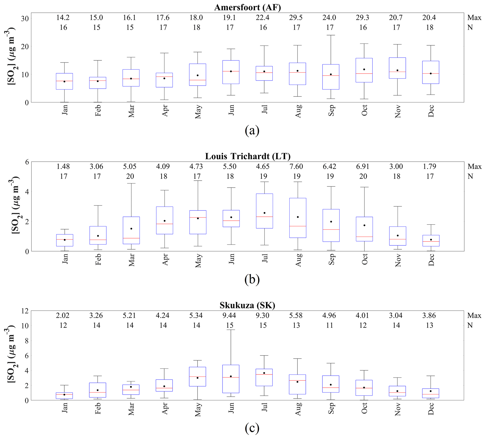
Figure 3 Monthly SO₂ concentrations measured at (a) AF from 1997 to 2015, (b) LT from 1995 to 2015 and (c) SK from 2000 to 2015. The red line of each box represents the median; the top and bottom edges of the box represent the 25th and 75th percentiles, respectively; the whiskers are ±2.7σ (99.3 % coverage if the data have a normal distribution); and the black dots represent the averages. The maximum concentrations and the number of measurements (N) are presented at the top.

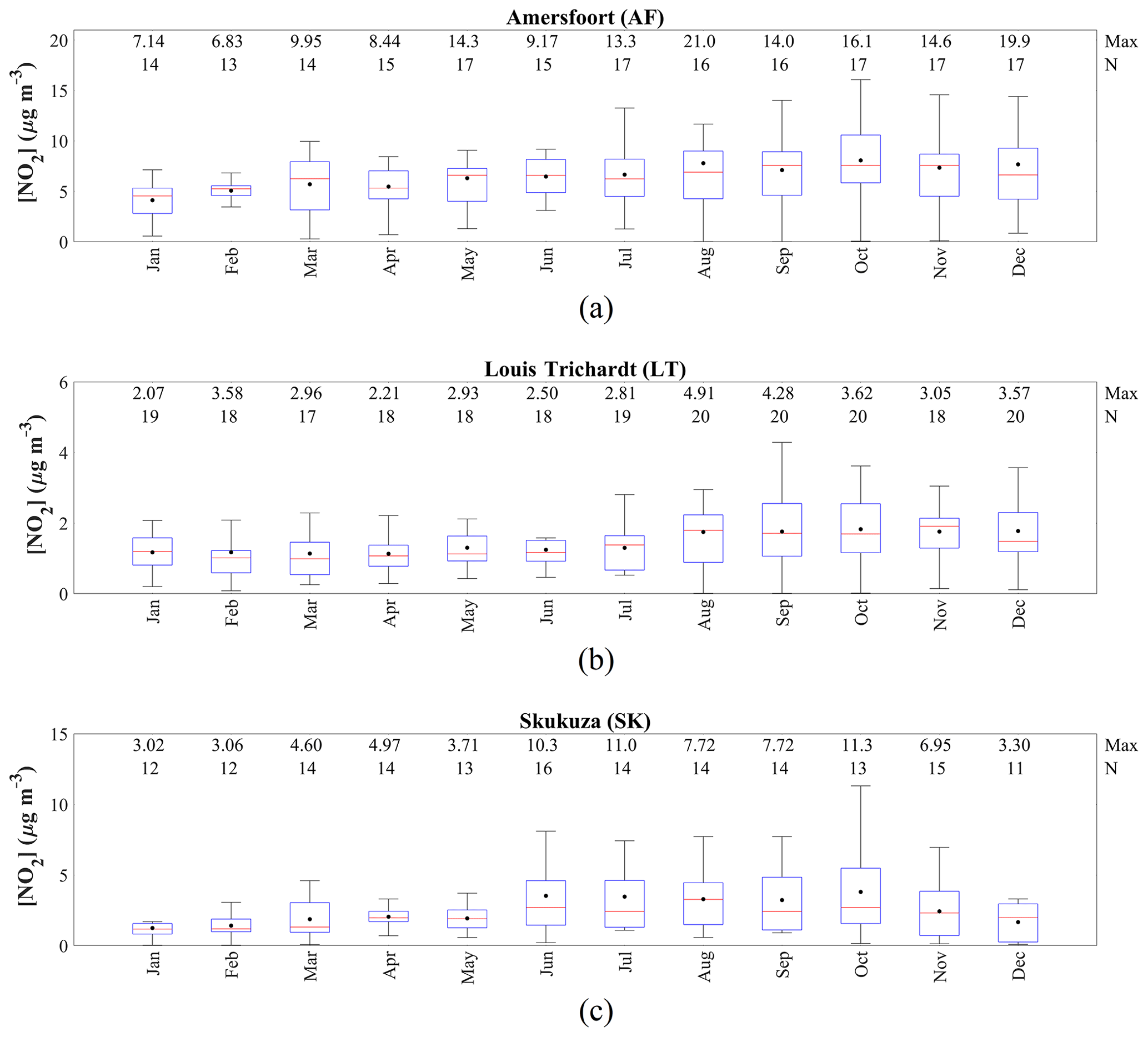
Figure 4 Monthly NO₂ concentrations measured at (a) AF from 1997 to 2015, (b) LT from 1995 to 2015 and at (c) SK from 2000 to 2015. The red line of each box represents the median; the top and bottom edges of the box represent the 25th and 75th percentiles, respectively; the whiskers are ±2.7σ (99.3 % coverage if the data have a normal distribution); and the black dots represent the averages. The maximum concentrations and the number of measurements (N) are presented at the top.

Figure 5 Monthly O₃ concentrations measured at (a) AF from 1997 to 2015, (b) LT from 1995 to 2015 and (c) SK from 2000 to 2015. The red line of each box represents the median; the top and bottom edges of the box represent the 25th and 75th percentiles, respectively; the whiskers are ±2.7σ (99.3 % coverage if the data have a normal distribution); and the black dots represent the averages. The maximum concentrations and the number of measurements (N) are presented at the top.

The inter-annual variability of SO₂, NO₂ and O₃ levels is presented in Figs. 6, 7 and 8, respectively, for AF, LT and SK. Noticeable from the SO₂ and NO₂ inter-annual fluctuations at all three sites is that the annual average SO₂ and NO₂ concentrations decreased up until 2003/2004 and 2002, respectively, which is followed by a period during which levels of SO₂ and NO₂ increased up until 2009 and 2007, respectively. After 2009, annual average SO₂ concentrations remained relatively constant, while NO₂ showed relatively large inter-annual variability, with annual NO₂ concentrations reaching a maximum in 2011 and 2012. These observed periods of decreased and increased SO₂ and NO₂ levels are also indicated by the 3-year moving averages of the annual mean SO₂ and NO₂ concentrations at all three sites. Since these trends are observed at all three sites, located several hundred kilometres apart in the north-eastern interior, these inter-annual trends seem real and not merely like a localized artefact. Furthermore, monthly SO₂ and NO₂ measurements conducted at the Cape Point Global Atmosphere Watch station on the western coast of South Africa also indicate similar periods of increase and decrease in SO₂ and NO₂ levels (Swartz et al., 2020). Although annual O₃ concentrations indicate inter-annual variances, annual average O₃ concentrations remained relatively constant at all three sites, with the exception of a decreasing trend observed from 1995 to 2001 at LT, corresponding to the period during which SO₂ and NO₂ decreased. Similar to seasonal variances, inter-annual fluctuations can also be ascribed to changes in meteorological conditions and/or variances in source contribution. Conradie et al. (2016), for example, indicated that rain samples collected from 2009 to 2014 at these three sites had higher ${\mathrm{SO}}_{\mathrm{4}}^{\mathrm{2}-}$ and ${\mathrm{NO}}_{\mathrm{3}}^{-}$ concentrations compared to rain samples collected in 1986 to 1999 and 1999 to 2002, which is attributed to increased energy demand and a larger vehicular fleet associated with economic and population growth.

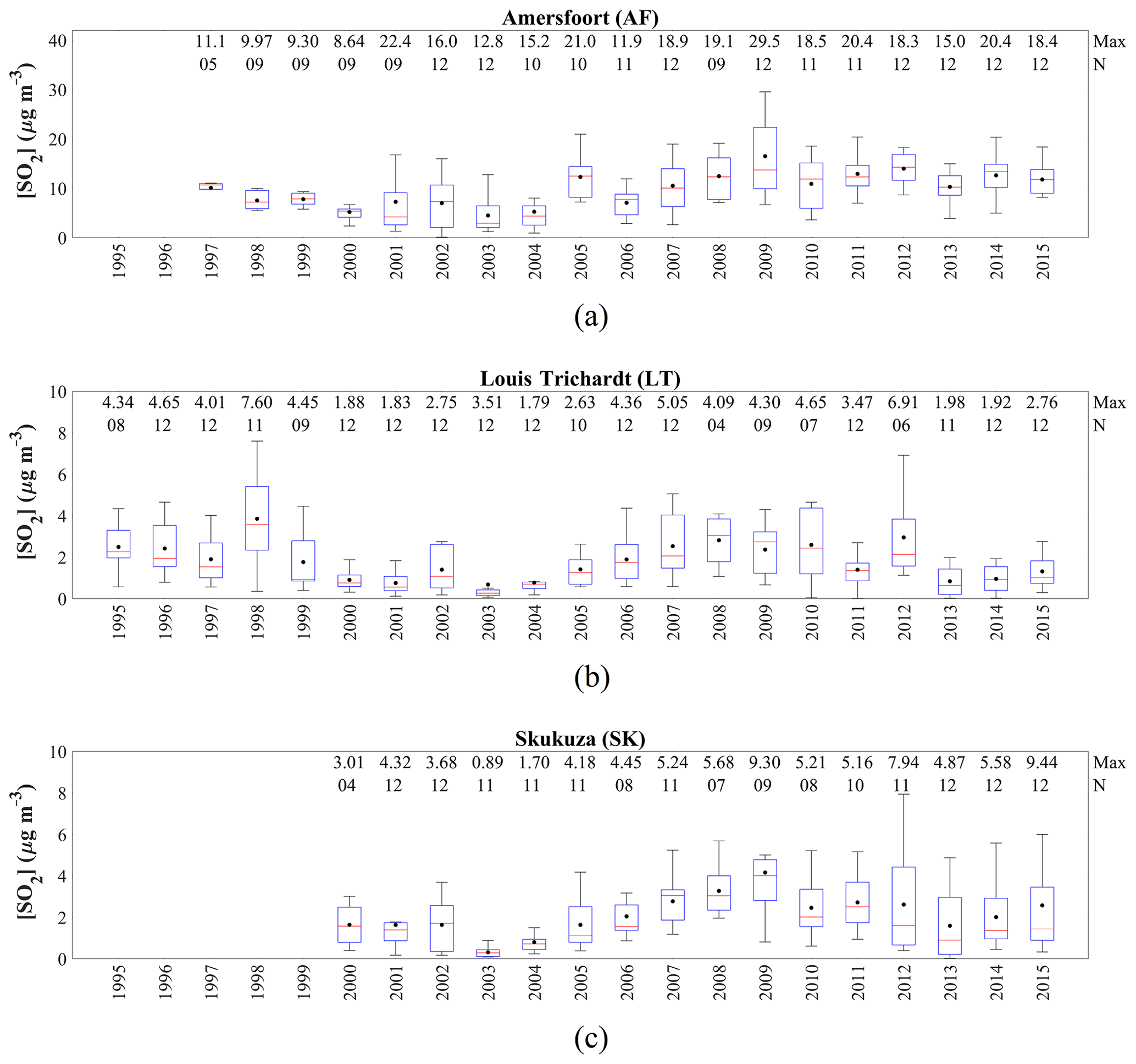
Figure 6 Annual SO₂ concentrations at (a) AF, (b) LT and (c) SK. The red line of each box represents the median; the top and bottom edges of the box represent the 25th and 75th percentiles, respectively; the whiskers are ±2.7σ (99.3 % coverage if the data have a normal distribution); and the black dots represent the averages. The maximum concentrations and the number of measurements (N) are presented at the top.

Figure 7 Annual NO₂ concentrations at (a) AF, (b) LT and (c) SK. The red line of each box represents the median; the top and bottom edges of the box represent the 25th and 75th percentiles, respectively; the whiskers are ±2.7σ (99.3 % coverage if the data have a normal distribution); and the black dots represent the averages. The maximum concentrations and the number of measurements (N) are presented at the top.

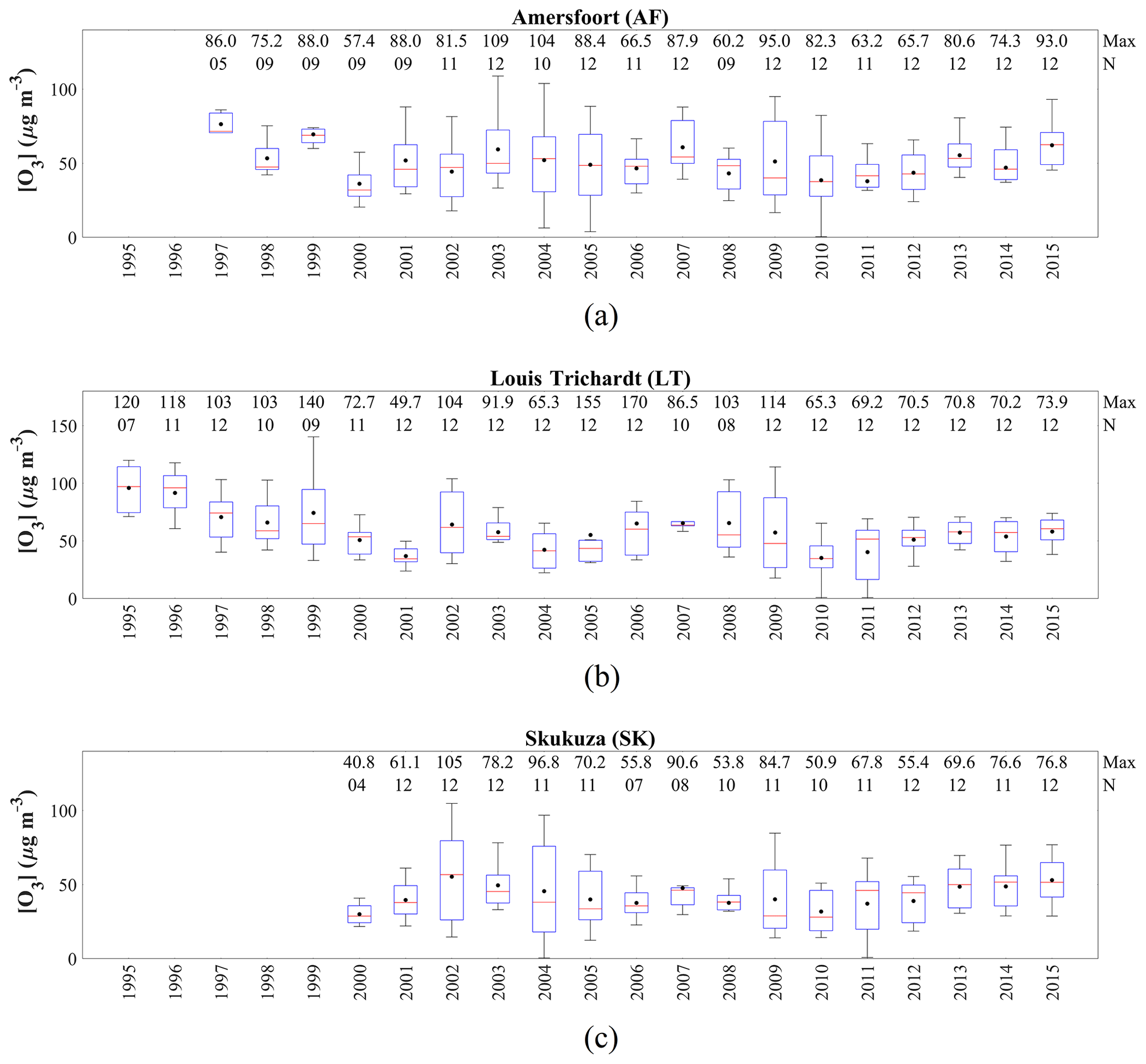
Figure 8 Annual O₃ concentrations at (a) AF, (b) LT and (c) SK. The red line of each box represents the median; the top and bottom edges of the box represent the 25th and 75th percentiles, respectively; the whiskers are ±2.7σ (99.3 % coverage if the data have a normal distribution); and the black dots represent the averages. The maximum concentrations and the number of measurements (N) are presented at the top.

3.2 Statistical modelling of variability

3.2.1 Sulfur dioxide (SO₂)

The SO₂ concentrations calculated with the MLR model are compared to measured SO₂ levels in Fig. 9 for AF (Fig. 9a), LT (Fig. 9b) and SK (Fig. 9c). In each panel, the RMSE differences between measured and modelled SO₂ concentrations are presented as a function of the number of independent variables included in the model (i and ii), while the differences between modelled and measured SO₂ levels for each sample are also indicated (iii). As indicated above, in the initial run of the model, only global factors were included (i and iii), after which all factors (local, regional and global) were incorporated in the model (ii and iii). In Table 1, the coefficients and RIW% of each of the independent variables are included in the optimum MLR equation containing all global factors, as well as in the optimum MLR equation when all local, regional and global factors are included. It is evident from Fig. 9a.iii, b.iii and c.iii that the correlations between measured and modelled SO₂ levels are significantly improved when all factors are considered in the MLR model compared to only including global factors at all three sites. The R² values are improved from 0.122 to 0.330, 0.078 to 0.257 and 0.100 to 0.389 at AF, LT and SK, respectively. Although relatively weak correlations are observed between modelled and measured SO₂ levels, the general trend of the measured SO₂ concentrations is mimicked by the modelled values, even when only global factors are included in the MLR model. In addition, the R² values at AF and SK when all factors are considered (0.330 and 0.389) can be considered moderate correlations (Kleynhans et al., 2017). It also seems that very high and low SO₂ levels are underestimated by the model. Swartz et al. (2020) attributed differences between monthly concentrations of species measured with passive samplers at Cape Point (CPT) GAW and modelled levels to the limitations associated with the use of passive samplers.

Figure 9 (i, ii) RMSE differences between modelled and measured SO₂ concentrations as a function of the number of independent variables included in the model, as well as a comparison between modelled and measured SO₂ levels (iii) for global force factors only (GFF) and for global, regional and local factors (RFF) determined for AF (a), LT (b) and SK (c).

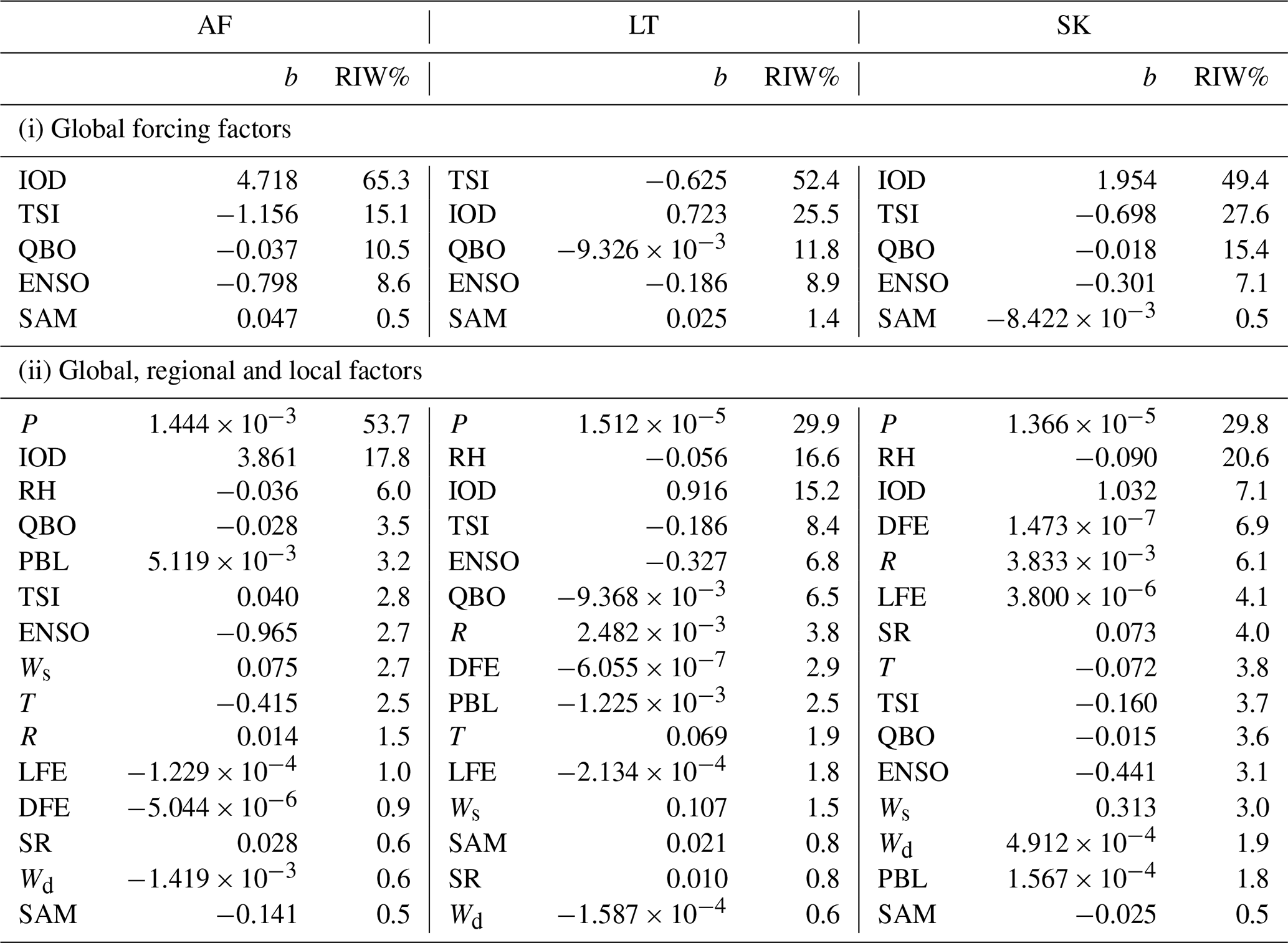
Table 1 Regression coefficients (b) and relative-importance weight percentage (RIW%) of each independent variable included in the MLR model to calculate SO₂ concentrations at AF, LT and SK.

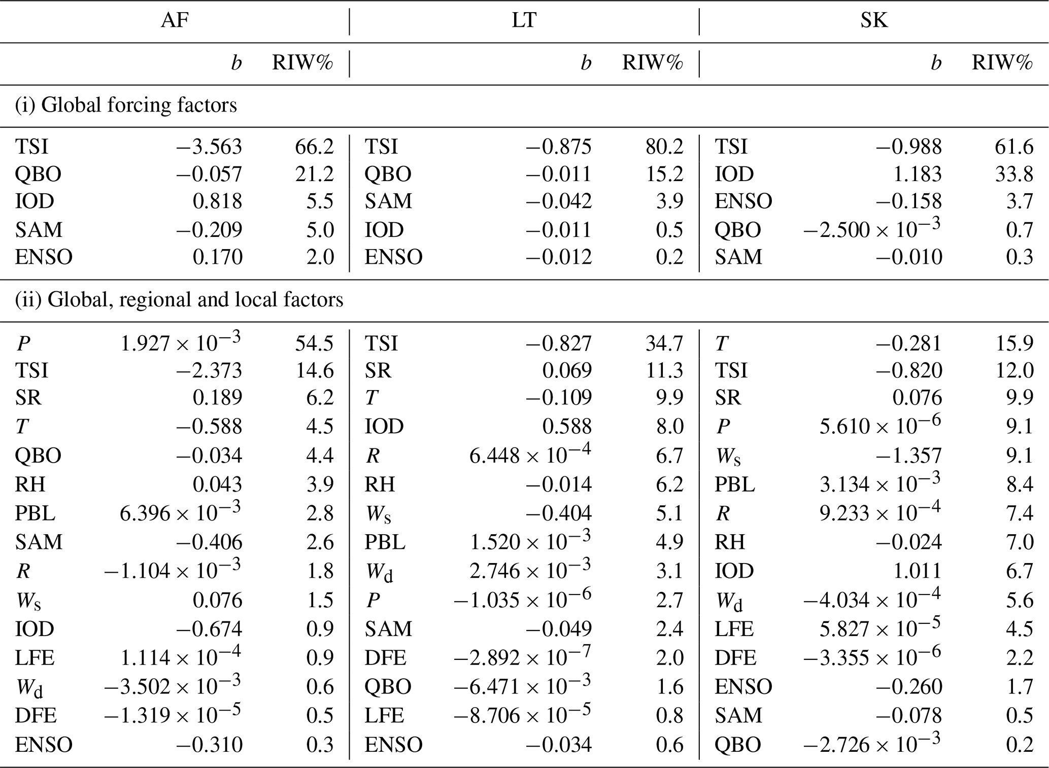
The interdependencies between TSI and QBO at AF and LT, as well as TSI and IOD at SK, yielded the largest decreases in RMSE when only global parameters were considered. The RIW% calculated for these parameters in the optimum MLR equation containing all global factors also indicates that these factors are the most significant. When all factors (local, regional and global) were considered in the model, the combinations between P, TSI, SR and T at AF; TSI, SR, IOD and R at LT; and T, TSI, P and W_s at SK contributed to the most significant decrease in RMSE for each of the sites. According to the RIW% calculated for each parameter in the optimum MLR equation containing all factors P (54.5 %) and TSI (14.6 %) at AF; TSI (34.7 %), SR (11.3 %), T (9.9 %) and IOD (8.0 %) at LT; and T (15.9 %), TSI (12.0 %), SR (9.9 %), P (9.1 %) and W_s (9.1 %) at SK were the most important factors contributing to variances. From the MLR model, it is evident that global meteorological factors contribute to SO₂ variability at each of these sites located in the north-eastern interior of South Africa. The model also indicates that the influence of global factors is more significant at the rural background site LT, where TSI made the largest contribution to the modelled value, while IOD also made a relatively important contribution. Although TSI was the second most significant factor at AF and SK, local and regional parameters were more important to variances in modelled SO₂ levels at these sites.

Population growth had the most substantial contribution to the dependent variable at the industrially influenced AF, which is indicative of the impacts of increased anthropogenic activities and energy demand in this region. Therefore, it is most likely that the observed inter-annual variability observed at AF, i.e. periods of decreased and increased SO₂ levels, can mainly be attributed to changes in source contribution. The decrease in SO₂ concentrations up until 2003/2004 is associated with a period following 1994 (when the new democracy was established), during which many companies obtained environmental accreditation (ISO 14000 series; ISO, 2015) and implemented mitigation technologies in order to comply with international trade requirements, e.g. certain large metallurgical smelters applied desulfurization technologies (e.g. Westcott et al., 2007). The period was characterized by an increased awareness of air pollution and its impacts in South Africa. However, it seems that these improvements made with regard to air pollution were offset from 2003/2004 due to rapid economic growth associated with increased industrial activities, e.g. increased production by pyrometallurgical industries (ICDA, 2012), as well as the increase in population growth accompanied by higher energy demand (Vet et al., 2014). In Fig. A4, the South African population and GDP (gross domestic product) from 1995 to 2015 according to the World Bank (World Bank, 2019) are presented together with the electricity generation (EG) in South Africa during this period as indicated by the International Energy Agency (International Energy Agency, 2020). A continuous growth in population is observed from 1995 to 2015, while the GDP trend reflects economic growth during this period corresponding to the observed periods of decreased and increased SO₂ concentrations. A general increase in electricity production over this period is also evident. Electricity consumption is a good indicator of increased anthropogenic activities, with Inglesi-Lotz and Blignaut (2011) indicating that electricity consumption in South Africa increased by 131 024 GWh from 1993 to 2006. In 2007/2008, the global financial crisis occurred, which forced numerous South African commodity-based producers (e.g. platinum group metal, base metal, ferrochromium, ferromanganese, ferrovanadium and steel smelters) to completely discontinue production. Ferrochromium production in South Africa, for instance, decreased by approximately 35 % from 2007 to 2009 (ICDA, 2013), while energy consumption in the manufacturing sector dropped by approximately 34 % from 2007 to 2008 (Statistics South Africa, 2012). Furthermore, these variances in source contribution associated with anthropogenic activities are also observed at LT and SK, distant from the major sources, due to these sites also being impacted by the regional circulation of air masses passing over major sources, as indicated in Fig. 2. In addition, the RIW% associated with P (9.1 %) in the optimum MLR equation containing all factors at SK is also indicative of not only the influence of population growth within the source region (Fig. 1) but also the increased populations of rural communities on the border of the Kruger National Park. Maritz et al. (2019) attributed higher organic and elemental carbon concentrations measured at SK to increased household biomass burning by these rural communities.

Temperature had the largest contribution to the variances of the modelled SO₂ at SK, while it was also an important parameter at LT. In addition, the source region (SR) factor made significant contributions to the dependent variable at SK and LT, while it also made a relative contribution at AF. These two factors are indicative of the influence of changes in local and regional meteorological conditions on SO₂ concentrations, as well as the important influence of air mass movement over the source region. The contribution of SR at all the sites indicated that months and/or years coinciding with these sites being more frequently impacted by air masses passing over the defined source region (Fig. 1) corresponded to increased SO₂ concentrations, while it also substantiates the aforementioned deduction that increased anthropogenic activities in the source region also influenced LT and SK. As indicated in Sect. 3.1, SK and LT revealed the expected higher SO₂ levels during winter, while AF had a less distinct seasonal pattern. Therefore, the strong negative correlation between temperature and modelled SO₂ concentrations at SK and LT, i.e. higher SO₂ levels associated with lower temperature, reflects the influence of local and regional meteorology on monthly SO₂ variability, i.e. build-up of pollutant concentrations during winter. At SK, the influence of local meteorology is also indicated by the relatively strong negative correlation to W_s, i.e. more stable conditions in winter coinciding with higher SO₂ concentrations. Furthermore, the influence of the rural communities in proximity of SK on SO₂ levels is also signified by T being the most significant factor contributing to modelled SO₂ values at this site. The less distinct seasonal pattern at AF can be attributed to the proximity of AF to the industrial SO₂ sources, with the major point sources consistently emitting the same levels of SO₂ throughout the year. Therefore, the average monthly SO₂ concentrations measured with passive samplers at AF do not reflect the influence of local and regional meteorology on atmospheric SO₂ concentrations.

The slopes of the trend lines of SO₂ values calculated when only global factors were included in the model did not correspond with the trend lines of the measured SO₂ concentrations at all the sites, with the exception of LT that showed slightly better correlations, signifying the stronger influence of global factors at this site (Fig. 9a.iii, b.iii and c.iii). However, the slopes of the linear regression trend lines for the measured SO₂ concentrations and the modelled SO₂ levels when all the factors are included in the model are exactly the same at AF, LT and SK when the same period is considered for both the modelled and measured values. A positive slope for the 19-year trend line for measured SO₂ concentrations is observed at AF (Fig. 9a.iii), indicating an increase in SO₂ levels over the 19-year sampling period, i.e. 0.43 µg m⁻³ yr⁻¹. An increase in SO₂ concentration, i.e. 0.09 µg m⁻³ yr⁻¹, is also determined for the 16-year measurement period at SK (Fig. 9b.iii), which is significantly smaller than the upward trend at AF. In contrast to AF and SK, LT indicates a slight net negative slope with SO₂ decreasing on average by 0.03 µg m⁻³ yr⁻¹ during the 21-year sampling period (Fig. 9c.iii). The 19- and 21-year datasets at AF and LT also allowed for the calculation of decadal trends, which were determined to be 5.24 µg m⁻³ per decade (average SO₂ concentrations from 1997 to 2006 were 7.20 µg m⁻³, and average SO₂ concentrations from 2007 to 2015 were 12.44 µg m⁻³) and 0.18 µg m⁻³ per decade (average SO₂ concentrations from 1995 to 2004 were 1.64 µg m⁻³, and average SO₂ concentrations from 2005 to 2014 were 1.82 µg m⁻³), respectively, for the 2 decades. Trend lines are also presented for the periods characterized by increased (1995, 1997 to 2003) and decreased (2004 to 2008/2009) SO₂ concentrations at LT and AF. The average annual trend between 1997 and 2003 at AF was −0.53 µg m⁻³ yr⁻¹, while the annual trend from 2004 to 2009 was 1.87 µg m⁻³ yr⁻¹. At LT, the average annual SO₂ concentrations decreased by −0.26 µg m⁻³ yr⁻¹ from 1995 to 2002 and increased by 0.37 µg m⁻³ yr⁻¹ from 2003 to 2007.

3.2.2 Nitrogen dioxide (NO₂)

In Fig. 10, the measured NO₂ concentrations are related to the modelled NO₂ levels, while Table 2 presents the coefficients and RIW% of each of the independent variables included in the optimum MLR equation modelling NO₂ concentrations. Similar to SO₂, the relationships between measured and modelled NO₂ are also significantly improved when local, regional and global factors are included in the model at all three sites (Fig. 10a.iii, b.iii and c.iii). However, inclusion of only global factors in the model yielded modelled NO₂ concentrations that mimicked the general measured NO₂ trend. The R² values, when only global factors are included, i.e. 0.171, 0.170 and 0.099 at AF, LT and SK, respectively, are enhanced to 0.498, 0.468 and 0.362 at AF, LT and SK, respectively, when all factors are considered in the MLR model. The R² values, when all factors are included, especially AF and LT, can be considered relatively good correlations (Sheskin, 2003). In general, modelled NO₂ concentrations corresponded well with the observed variances in measured NO₂ levels when all factors are included in the model at all three sites, with the exception of very high NO₂ concentrations.

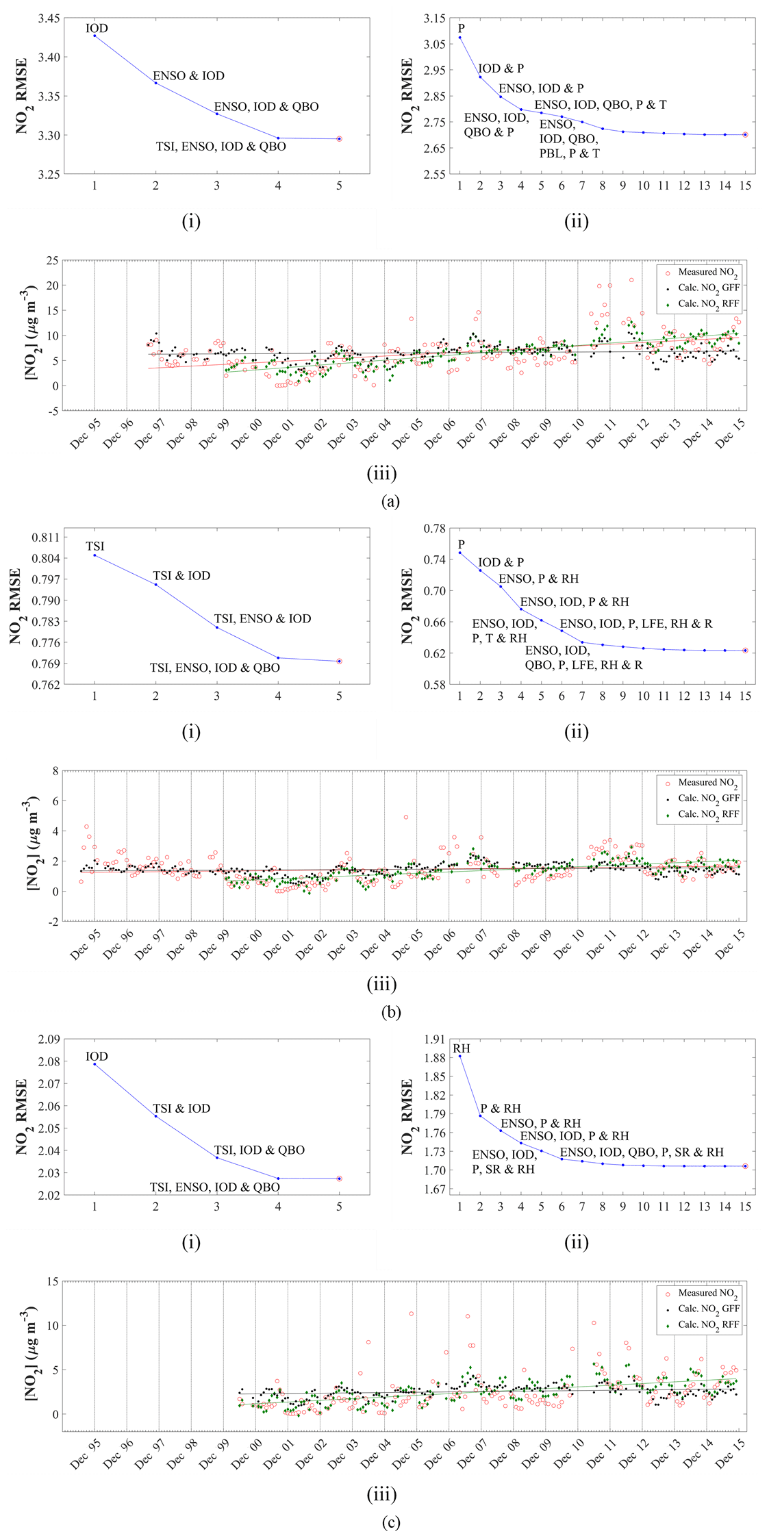
Figure 10 (i, ii) RMSE differences between modelled and measured NO₂ concentrations as a function of the number of independent variables included in the model, as well as a comparison between modelled and measured NO₂ levels (iii) for global force factors only (GFF) and for global, regional and local factors (RFF) determined for AF (a), LT (b) and SK (c).

Table 2 Regression coefficients (b) and relative-importance weight percentage (RIW%) of each independent variable included in the MLR model to calculate NO₂ concentrations at AF, LT and SK.

The annual trend calculated from the slope of the 19-year measured NO₂ dataset at AF indicates an annual increase of 0.33 µg m⁻³ yr⁻¹, while the 16-year measured NO₂ concentrations indicate an upward trend of 0.19 µg m⁻³ yr⁻¹ at SK. The trend line of measured NO₂ concentrations at LT also indicated a marginal increase, i.e. 0.02 µg m⁻³ yr⁻¹ in NO₂ levels over the 21-year sampling period. Decadal trends were determined to be 3.43 µg m⁻³ per decade (average NO₂ concentrations from 1997 to 2006 were 4.86 µg m⁻³, and average NO₂ concentrations from 2007 to 2015 were 8.29 µg m⁻³) and 0.45 µg m⁻³ per decade (average NO₂ concentrations from 1995 to 2004 were 1.23 µg m⁻³, and average NO₂ concentrations from 2005 to 2014 were 1.68 µg m⁻³), respectively, for the 2 decades. Trend lines were also calculated for the periods coinciding with increases and decreases in measured NO₂ concentrations at AF and LT. The average annual trend between 1997 and 2003 at AF was −0.26 µg m⁻³ yr⁻¹, while the annual trend from 2004 to 2009 was 0.37 µg m⁻³ yr⁻¹. At LT, the average annual NO₂ concentrations decreased by −0.29 µg m⁻³ yr⁻¹ from 1995 to 2002 and increased by 0.28 µg m⁻³ yr⁻¹ from 2003 to 2007. Similar to SO₂, the slopes of the linear regression trend lines for the measured NO₂ concentrations and the modelled NO₂ levels when all the factors are included in the model are exactly the same at AF, LT and SK (Fig. 10a.iii, b.iii and c.iii). However, with the exception of LT, the slopes of the trend lines of NO₂ levels calculated including only global factors in the model did not correspond with the trend lines of the measured NO₂ concentrations, indicating the significance of local and regional factors on measured NO₂ concentrations (Fig. 10a.iii, b.iii and c.iii).

The RMSE differences between the modelled and measured NO₂ concentrations (Fig. 10a.i, b.i and c.i) indicated that the linear combination between most of the global force factors, i.e. IOD, TSI, QBO and ENSO, resulted in the largest decrease in RMSE when only global force factors were included. The RIW% listed in Table 2 for the optimum MLR equation, including only global factors, indicates that IOD (65.3 % and 49.4 %, respectively) was the most significant parameter at AF and SK, while TSI (52.4 %) was the most important factor at LT. The inclusion of local, regional and global factors in the MLR model indicated that the interdependencies between P, IOD, QBO, ENSO and T at AF; P, RH, IOD, ENSO and T at LT; and P, RH, IOD and ENSO at SK yielded the largest decrease in RMSE difference. The RIW% determined for each independent variable in the optimum MLR equation containing all parameters indicated the most important factors explaining variances in the dependent variable (i.e. NO₂ levels) were P (53.7 %) and IOD (17.8 %) at AF; P (29.9 %), RH (16.6 %) and IOD (15.5 %) at LT; and P (29.8 %) and RH (20.6 %) at SK. It is evident from these interdependencies of the dependent variable and RIW% of parameters included in the MLR model that local and regional factors were more significant to NO₂ variability at AF, LT and SK, while global meteorological factors also contributed to variances in NO₂ levels.

Population growth made the most significant contribution to modelled NO₂ concentrations at all three sites and not only at AF, as observed for SO₂. Therefore, the influence of increased population growth and associated anthropogenic activities is reflected in ambient NO₂ concentrations modelled for the entire north-eastern interior region. Therefore, the periods coinciding with decreased (up until 2002) and increased (2003 to 2007) NO₂ inter-annual variability can be attributed to similar variances in source contribution, as discussed above for SO₂, with regional circulation of air masses passing over major sources also influencing LT and SK (Fig. 2). However, the significant contribution of population growth to the modelled NO₂ levels at two rural background sites (LT and SK) also points to increased household combustion associated with enlarged populations within rural communities being a major source of NO₂ in this part of South Africa. The influence of increased seasonal household combustion is also indicated by higher NO₂ concentrations determined in June and July at SK (Fig. 4), which also signifies the impacts of the growing rural communities in proximity of SK.

RH made the second most important contribution in explaining variances in modelled NO₂ concentrations at LT and SK, while it was the third most important factor at AF as indicated by RIW%. Therefore, RH can be considered the factor representing the influence of changes in local and regional meteorology at these sites. Although T was indicated as a factor included in the linear combination of parameters yielding the largest decrease in RMSE at AF and SK, its relative importance in explaining modelled variances is not indicated by its RIW% in Table 2. The strong negative correlation with RH is indicative of increased NO₂ corresponding with months (or years) when dry meteorological conditions prevail, i.e. winter and early spring months in the north-eastern interior of South Africa. As indicated in Fig. 4, higher NO₂ concentrations did correspond with dry months (August to November) associated with increased biomass burning. However, the model does not reflect significant contributions of the two parameters included in the model to represent biomass burning, i.e. LFE and DFE to NO₂ variability with relatively higher RIW% observed for DFE (6.9%) and LFE (4.1 %) only at SK. Furthermore, higher annual average NO₂ concentrations observed in 2011 and 2012 (Fig. 7) at all the sites are also not explained by the MLR model.

3.2.3 Ozone (O₃)

Modelled and measured O₃ concentrations at AF, LT and SK are presented in Fig. 11, while Table 3 presents the coefficients and the RIW% of independent variables considered in the optimum MLR equation. When only global factors are considered in the model, the linear combinations between ENSO, TSI, IOD and SAM at AF; ENSO, TSI and SAM at LT; and ENSO and IOD at SK resulted in the largest RMSE differences between measured and modelled O₃ levels. However, according to RIW% values calculated, the most significant global factor contributing to O₃ variability was ENSO at all three sites (84.1 %, 41.8 % and 96.7 % at AF, LT and SK, respectively). The interdependencies between parameters when local, regional and global factors were included in the models, as well as the RIW% contributions of all factors included in the optimum MLR equation, also indicated the significance of ENSO in explaining variances in atmospheric O₃ concentrations at all three sites. Interdependencies between ENSO, IOD, PBL, LFE and R at AF; ENSO, PBL, T, RH and R at LT; and ENSO, PBL, T, RH and R at SK yielded the largest decrease in RMSE differences between measured and modelled O₃ levels, while RIW% indicated that the largest contributions made by factors explaining O₃ variability were ENSO (22.6 %), R (14.6 %) and W_s (10.1 %) at AF; RH (23.1 %), ENSO (16.8 %) and T (10.5 %) at LT; and T (24.6 %), ENSO (19.5 %), RH (11.3 %) and DFE (10.1 %) at SK when local, regional and global factors were included in the model.

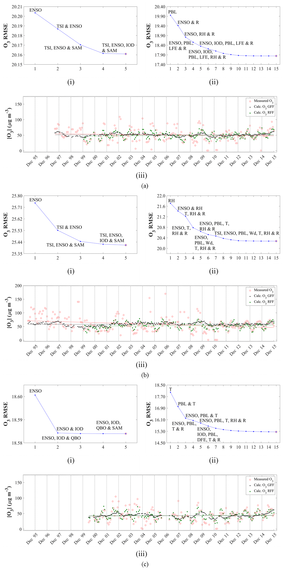
Figure 11 (i, ii) RMSE differences between modelled and measured O₃ concentrations as a function of the number of independent variables included in the model, as well as a comparison between modelled and measured O₃ levels (iii) for global force factors only (GFF) and for global, regional and local factors (RFF) determined for AF (a), LT (b) and SK (c).

Table 3 Regression coefficients (b) and relative-importance weight percentage (RIW%) of each independent variable included in the MLR model to calculate O₃ concentrations at AF, LT and SK.

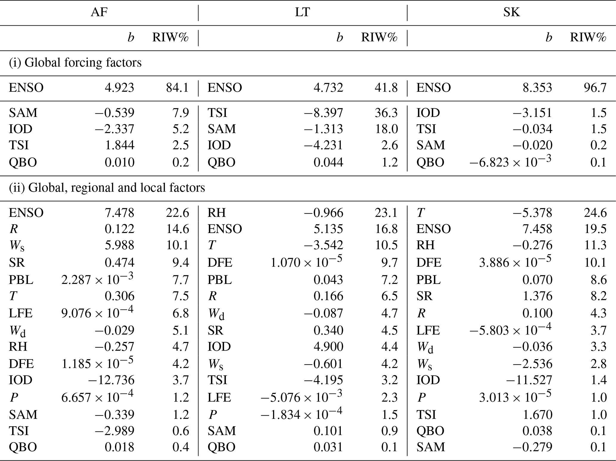
The significant contribution of ENSO on variances of the dependent variable (modelled O₃ concentrations) is evident at all three sites, with RIW% indicating ENSO to be the major factor at AF and the second most important factor at LT and SK when local, regional and meteorological factors are included in the model. Therefore, inter-annual variability in O₃ concentrations can most likely be attributed to ENSO cycles. El Niño periods are associated with drier and warmer conditions in the South African interior, which are conducive to O₃ formation, while cloudy and increased rainfall conditions related to La Niña hinder O₃ production (Balashov et al., 2014). Balashov et al. (2014) indicated that surface O₃ concentrations on the South African Highveld are sensitive to ENSO, with the El Niño period amplifying O₃ formation. The influence of local and regional meteorological conditions is also indicated by the substantial contributions of R and W_s at AF, as well as T and RH at LT and SK on modelled O₃ levels. At LT, RH made the most substantial contribution to the dependent variable, while T made the most significant contribution to modelled O₃ levels. The negative correlation to T and RH at LT and SK is indicative of higher O₃ concentrations corresponding with drier colder months, as indicated in Fig. 5. Laban et al. (2018) indicated the significance of RH to surface O₃ concentrations in the north-eastern part of South Africa through the statistical analysis of in situ O₃ measurements conducted in this region, with RH also negatively correlated to surface O₃ levels. The positive correlation to R and W_s at AF reflects higher O₃ concentrations measured during late spring and summer at AF, i.e. October to January, which is a period associated with increased rainfall and less stable meteorological conditions (Fig. 5). The influence of regional open biomass burning during late winter and spring (August to November) on surface O₃ concentrations in this part of South Africa is indicated by the relatively significant contribution of DFE on modelled O₃ concentrations at LT and SK. A recent paper reporting tropospheric O₃ levels measured at four sites in the north-eastern interior of South Africa indicated that O₃ is a regional problem, with O₃ concentration measured at these four sites being similar to levels thereof measured at AF, LT and SK (Laban et al., 2018). A time series of O₃ levels measured from 2010 to 2015 at one of the sites presented by Laban et al. (2018) also indicated higher O₃ concentration corresponding to drier years associated with the ENSO cycle.

As indicated in Fig. 8, inter-annual O₃ concentrations at LT decreased from 1995 to 2001, which corresponded to the period when SO₂ and NO₂ concentrations decreased, as discussed in Sect. 3.1. This period of inter-annual decrease in O₃ levels is not reflected in the statistical model. Since LT is a rural background site with low NO_x emissions, it can be considered to be located in an NO_x-limited O₃ production regime, where O₃ concentrations correspond with NO_x concentrations, i.e. an increase or decrease with increasing or decreasing NO_x. Therefore, the decrease in O₃ concentrations from 1995 to 2001 can be attributed to decreasing NO₂ concentrations during this period and the factors influencing NO₂ concentrations at LT, i.e. mainly population growth, as discussed above (Sect. 3.2.2).

The comparisons between modelled and measured O₃ concentrations (Fig. 11a.iii, b.iii and c.iii) also indicated, as observed for SO₂ and NO₂, that the correlations are significantly improved when local, regional and global factors are included in the model. The R² values, when only global factors are included, i.e. 0.042, 0.048 and 0.094 at AF, LT and SK, respectively, are improved to 0.259, 0.241 and 0.389 at AF, LT and SK, respectively. These correlations can be considered relatively weak, with the exception of a moderate correlation at SK (Sheskin, 2003). These generally weaker correlations can be attributed to the complexity associated with tropospheric O₃ chemistry. Tropospheric O₃ is a secondary atmospheric pollutant with several factors contributing to its variability. In addition, Laban et al. (2018) indicated the significance of the precursor species CO to surface O₃ concentrations in the north-eastern interior of South Africa, which were not measured at any of the sites and included in the model. Swartz et al. (2020) also compared passively derived O₃ concentrations with active O₃ measurements and illustrated limitations associated with the use of passive samplers to determine O₃ concentrations. However, the general trend of measured O₃ concentrations is mimicked by the modelled O₃ values when local, regional and global factors are included in the model, while the overall trend is weakly followed when only global factors are included. Higher and lower O₃ concentrations are underestimated by the MLR model.

The trend lines for the O₃ concentrations measured during the entire sampling periods indicate slight negative slopes at AF and LT (Fig. 11a.iii and b.iii, respectively) and a small positive slope at SK (Fig. 11c.iii). Annual average decreases in O₃ levels of 0.37 and 1.20 µg m⁻³ yr⁻¹ were calculated at AF and LT, respectively, while an average annual increase of 0.21 µg m⁻³ yr⁻¹ was calculated at SK. However, in general, it seems that O₃ concentrations remained relatively constant at all three sites for the entire 19-, 21- and 16-year sampling periods at AF, LT and SK, respectively. Decadal trends of −3.46 (average O₃ concentrations from 1997 to 2006 were 52.56 µg m⁻³, and average O₃ concentrations from 2007 to 2015 were 49.10 µg m⁻³) and −9.15 µg m⁻³ per decade (average O₃ concentrations from 1995 to 2004 were 63.16 µg m⁻³, and average O₃ concentrations from 2005 to 2014 were 53.01 µg m⁻³) were calculated for AF and LT, respectively, for the 2 decades. Similar to SO₂ and NO₂, the slopes of the linear regression trend lines for the measured and modelled O₃ concentrations when local, regional and global factors are included are exactly the same at AF, LT and SK (Fig. 11a.iii, b.iii and c.iii), which indicates that measured and modelled O₃ trends compare well in spite of low R² values. In addition, relatively good correlations are observed between the slopes of the trend lines of measured O₃ concentrations and modelled O₃ values calculated when only global factors are included at all the sites, signifying the influence of global factors, especially ENSO, as indicated above, on O₃ variability (Fig. 11a.iii, b.iii and c.iii).

3.3 Contextualization

In order to contextualize the long-term SO₂, NO₂ and O₃ concentrations measured with passive samplers at AF, LT and SK located in the north-eastern interior of South Africa, the statistical spread of the concentrations of these species determined during the entire sampling period at each site are compared to average concentrations of these species determined with passive samplers during other studies in South Africa and Africa, as well as regional sites in other parts of the world. SO₂, NO₂ and O₃ concentrations determined in this study are related to levels reported elsewhere in Figs. 12, 13 and 14, respectively.

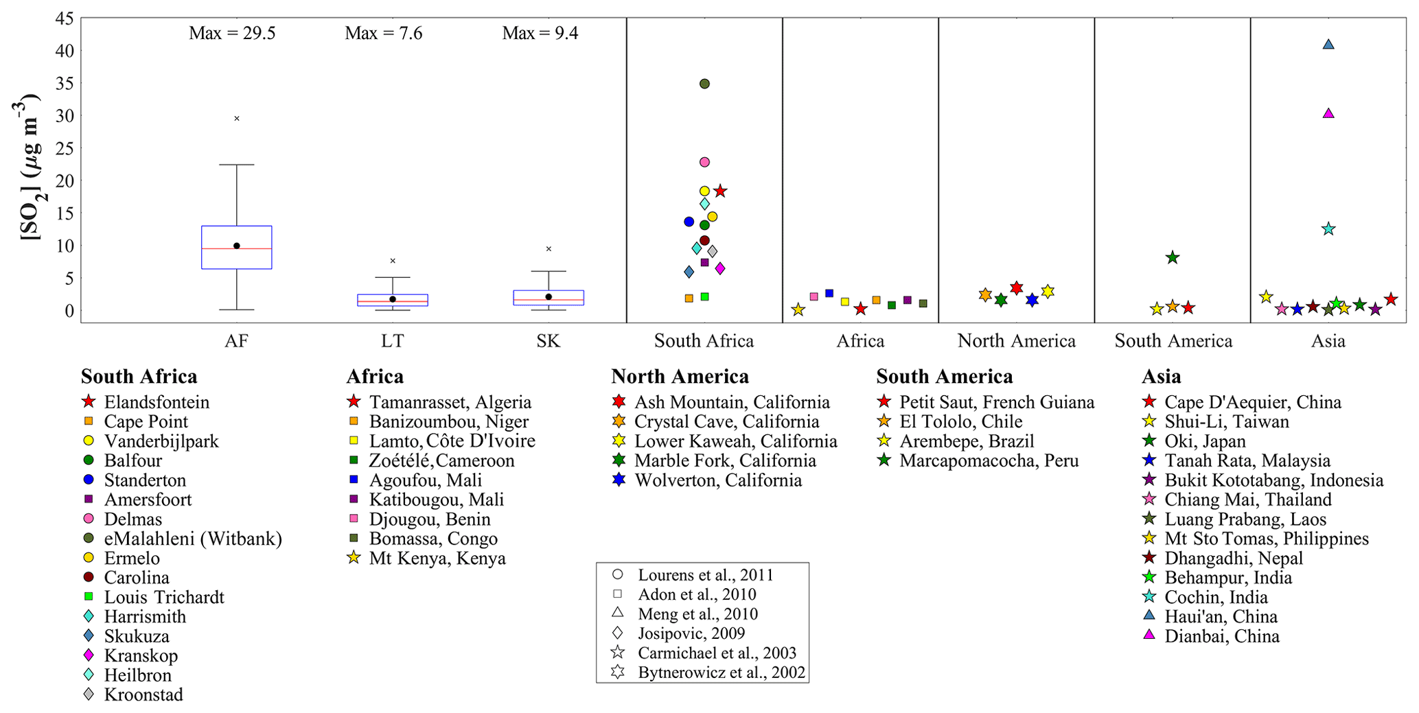
Figure 12 Statistical spread of SO₂ concentrations determined during the entire measuring period at each site compared to mean levels determined with passive samplers elsewhere. The red line of each box represents the median; the top and bottom edges of the box represent the 25th and 75th percentiles, respectively; the whiskers are ±2.7σ (99.3 % coverage if the data have a normal distribution); and the black dots represent the average concentrations.

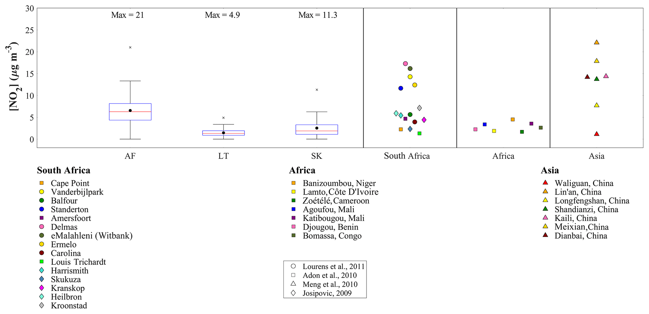
Figure 13 Statistical spread of NO₂ concentrations determined during the entire measuring period at each site compared to mean levels determined with passive samplers elsewhere. The red line of each box represents the median; the top and bottom edges of the box represent the 25th and 75th percentiles, respectively; the whiskers are ±2.7σ (99.3 % coverage if the data have a normal distribution); and the black dots represent the average concentrations.

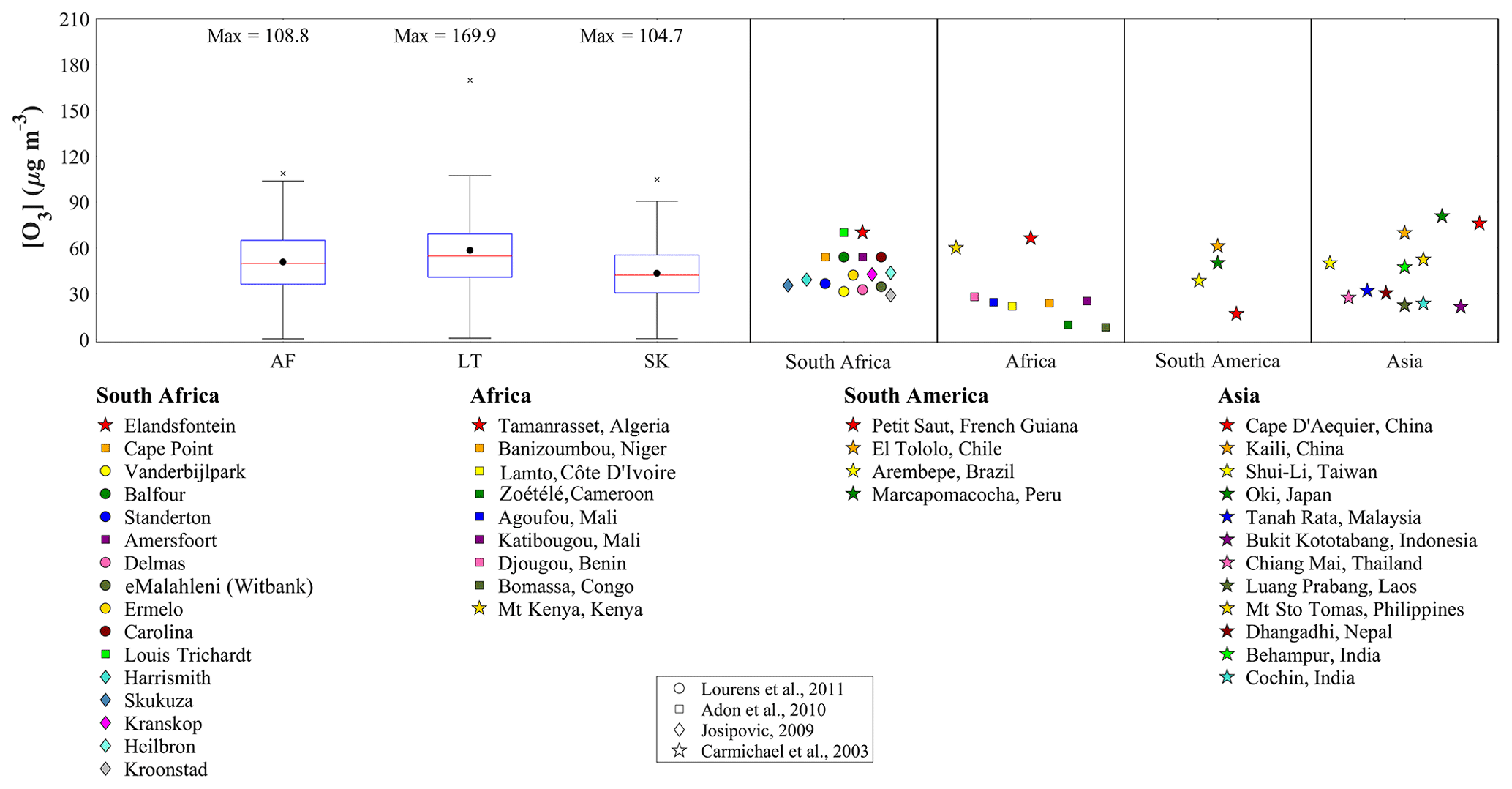
Figure 14 Statistical spread of O₃ concentrations determined during the entire measuring period at each site compared to mean levels determined with passive samplers elsewhere. The red line of each box represents the median; the top and bottom edges of the box represent the 25th and 75th percentiles, respectively; the whiskers are ±2.7σ (99.3 % coverage if the data have a normal distribution); and the black dots represent the average concentrations.

As expected, the average and median SO₂ concentrations determined at the industrially impacted AF (9.91 and 9.48 µg m⁻³, respectively) site were higher compared to average and median SO₂ levels determined at the rural background sites LT (1.70 and 1.35 µg m⁻³, respectively) and SK (2.07 and 1.60 µg m⁻³, respectively) for the entire sampling period at each site. Geospatial maps of SO₂ column amount in the planetary boundary layer and NO₂ tropospheric column density averaged over the period 2005 to 2015 over southern Africa (Figs. A5 and A6,' respectively) indicate higher average SO₂ and NO₂ concentrations being observed over the region where AF is located. Much lower average SO₂ and NO₂ concentrations are observed over the northernmost parts of the country, where LT is located, as well as the western region where SK is situated. Therefore, the influence of coal-fired power stations on SO₂ (and NO₂) levels measured at AF is evident. The average SO₂ levels at AF were similar to average SO₂ concentrations determined at other sites located in the Mpumalanga Highveld, for which the measurement period was from August 2007 to July 2008 (Lourens et al., 2011). However, the average SO₂ level at AF was significantly lower than the mean SO₂ levels at Elandsfontein, Delmas and eMalahleni (formerly Witbank). Elandsfontein and Delmas are situated within closer proximity to major industrial activities in the Mpumalanga Highveld, while eMalahleni (Witbank) is a relatively large urban area with numerous large industrial point sources (Lourens et al., 2011). In addition, the average SO₂ concentrations at Vanderbijlpark – an urban area located within the highly industrialized Vaal Triangle region – were also higher compared to levels thereof at AF. Average SO₂ concentrations determined at regional sites in South America and India, i.e. Marcapomacocha and Cochin, respectively, were also similar to mean SO₂ levels determined at AF (Carmichael et al., 2003). The measurement period of the Carmichael et al. (2003) study was 12 months, starting in September 1999 (Carmichael et al., 2003). SO₂ concentrations reported for two rural sites in China, i.e. Dianbai and Haui'an, were similar to SO₂ levels determined at eMalahleni (Witbank) (Meng et al., 2010). Meng et al. (2010) presented results obtained during a 2-year study that commenced in January 2007. The mean SO₂ concentrations determined at LT and SK were similar to average SO₂ concentrations determined at regional background sites in western and central African sites (Carmichael et al., 2003; Adon et al., 2010), as well as mean SO₂ levels determined at most of the regional sites in North America – measured between May and November 1999, South America and Asia (Bytnerowicz et al., 2002; Carmichael et al., 2003). Adon et al. (2010) presented ambient SO₂, NO₂ and O₃ concentrations measured from 1998 to 2007 at Katibougou in Mali, Banizoumbou in Niger, Lamto in Côte D'Ivoire and Zoétélé in Cameroon. The measurement periods for Agoufou in Mali and Djougou in Benin was from 2005 to 2007, while for Bomassa in Congo measurements were reported between 1998 and 2006 (Adon et al., 2010).

Similar to SO₂, the mean and median NO₂ levels determined for the respective sampling periods at each site were higher at AF (6.56 and 6.29 µg m⁻³, respectively) compared to mean and median levels thereof at LT (1.45 and 1.32 µg m⁻³, respectively) and SK (2.54 and 1.89 µg m⁻³, respectively). Relatively higher NO₂ concentrations were determined at SK compared to LT, which can be attributed to the influence of growing rural communities on the border of the Kruger National Park (Maritz et al., 2019). The mean NO₂ concentrations at AF were lower compared to most of the average NO₂ levels determined at other sites located in the Mpumalanga Highveld within closer proximity to industrial sources, while being similar to mean NO₂ concentrations measured at Balfour and Carolina. In addition, average NO₂ levels at AF were also lower-than-average NO₂ concentrations determined in the Vaal Triangle (Lourens et al., 2011). Average NO₂ concentrations determined at rural and regional sites in China were higher than mean NO₂ levels at AF, with the exception of Longfengshan that had similar NO₂ concentrations to AF (Meng et al., 2010), which reflects the scale of atmospheric pollution in China. The average NO₂ concentrations at LT and SK were also similar to mean NO₂ levels determined at regional sites in western and central African sites (Carmichael et al., 2003; Adon et al., 2010), as well as a remote site (Waliguan) in China (Meng et al., 2010).

The statistical distribution of O₃ concentrations determined at AF, LT and SK indicates similar surface O₃ levels at all three sites with marginally higher O₃ concentrations determined at LT (58.44 and 54.67 µg m⁻³, respectively) compared to AF (50.77 and 49.84 µg m⁻³, respectively) and SK (43.36 and 42.20 µg m⁻³, respectively). Higher O₃ levels are expected at the rural background LT site due to decreased O₃ titration compared to polluted regions, while LT is also impacted by aged air masses passing over the Mpumalanga Highveld source region as previously indicated. However, the regional O₃ problem in the South African interior is reflected by high O₃ concentrations also measured at the industrially influenced AF site, as well as similar O₃ levels determined at other sites in the Mpumalanga Highveld (Lourens et al., 2011). Laban et al. (2018) attributed high regional O₃ concentrations in the north-eastern interior of South Africa to the influence of household combustion and widespread open biomass burning impacting this region. In addition, the influence of rural communities is also reflected by the slightly lower average O₃ levels at SK. O₃ concentrations measured at western and central Africa sites were lower than South African O₃ levels (Adon et al., 2010), with the exception of Mt Kenya and a site in northern Africa that had similar O₃ concentrations (Carmichael et al., 2003). Similar O₃ concentrations were determined at the South American regional sites, except for Petit Saut, which had lower O₃ concentrations (Carmichael et al., 2003). Average O₃ levels determined at some of the regional Asian sites were in the same range as O₃ concentrations over the interior of South Africa, while certain sites in Asia had lower mean O₃ levels (Carmichael et al., 2003).

4 Summary and conclusions

In this study, long-term trends of atmospheric SO₂, NO₂ and O₃ concentrations measured with passive samplers at three sites located in the north-eastern interior of South Africa are presented. This paper illustrates the value of low-cost atmospheric sampling techniques in order to obtain long-term data, especially for regions restricted by logistical accessibility and limited capacity. A 19-year (1997 to 2015), 21-year (1995 to 2015) and 16-year (2000 to 2015) dataset for AF, LT and SK could be evaluated. Long-term temporal trends indicated seasonal and inter-annual variability at all three sites, which could be ascribed to changes in meteorological conditions and/or variances in source contribution. Inter-annual variability indicated periods up until 2003/2004 and 2002 during which SO₂ and NO₂ concentrations, respectively, decreased, followed by periods during which SO₂ and NO₂ levels increased up until 2009 and 2007, respectively. These long-term trends were assessed with an MLR model in order to establish the influence of sources, as well as local, regional and global meteorology on atmospheric SO₂, NO₂ and O₃ concentrations.

Interdependencies between local, regional and global parameters included in the statistical model indicated the influence of global meteorology on SO₂ variability at all three sites, especially at the rural background site LT. However, population growth was the most substantial factor in the statistical model at the industrially impacted AF site, while the significance of local and regional meteorology was also evident with T being the most significant factor at SK. The important contribution of population growth on modelled SO₂ levels at AF was indicative of the impact of increased anthropogenic activities and energy demand in the north-eastern interior of South Africa. Higher SO₂ concentrations associated with lower temperatures reflected the influence of pollution build-up during winter, while the influence of air masses passing over the source region is also evident at SK and LT. Although global parameters contributed to variances in NO₂ concentrations, local and regional factors made more substantial contributions to modelled NO₂ levels. The most significant factor explaining NO₂ variability at all three sites was population growth, while RH was the most important local and regional meteorological factor. Therefore, similar to SO₂, the influence of population growth and associated increases in anthropogenic activities in the north-eastern interior is also reflected in NO₂ levels, while the impacts of increased household combustion associated with growing rural communities are also evident, especially at SK. The negative correlation to RH indicates higher NO₂ levels associated with drier months, i.e. winter, which contribute to seasonal variances. ENSO was shown to make a significant contribution to modelled O₃ levels at all three sites, while the important influence of local and regional meteorological factors was also evident, especially through significant negative correlations with T and RH at SK and LT. Inter-annual O₃ variability in this part of South Africa can therefore most likely be attributed to ENSO cycles, while seasonal patterns are attributed changes in local and regional meteorology.

The decreases in SO₂ and NO₂ concentrations from 1995 were attributed to the implementation of mitigation policies by industries following the establishment of the new democracy in South Africa. However, these improvements were offset from 2002 due to rapid economic growth associated with increased industrial activities, as well as the increase in population growth accompanied by higher energy demand. The 19-year trend lines for SO₂ and NO₂ at AF indicated an increase in SO₂ and NO₂ concentrations over the 19-year sampling period. In addition, an upward trend in NO₂ levels was also evident at SK, signifying the influence of the growing rural communities on the border of the Kruger National Park. Marginal trends were observed for SO₂ at SK, as well as SO₂ and NO₂ at LT. Trend analysis of O₃ at all three sites indicated that O₃ concentrations remained relatively constant at all three sites for the entire 19-, 21- and 16-year sampling periods at AF, LT and SK, respectively.

As expected, SO₂ and NO₂ concentrations were higher at AF compared to levels thereof at the rural background sites LT and SK. SO₂ levels at AF were similar to levels of these species determined with passive samplers at other sites within the Mpumalanga Highveld with the exception of sites closer to the major industrial sources. NO₂ levels at AF were generally lower than NO₂ concentrations determined at sites within the source region, as well as lower than regional sites in China. SO₂ and NO₂ concentrations determined at LT and SK were similar to levels thereof determined with passive samplers at regional and rural sites in Africa and other parts of the world. The regional problem of O₃ in the interior of South Africa was also evident, with similar O₃ levels determined at all three sites.

Appendix A

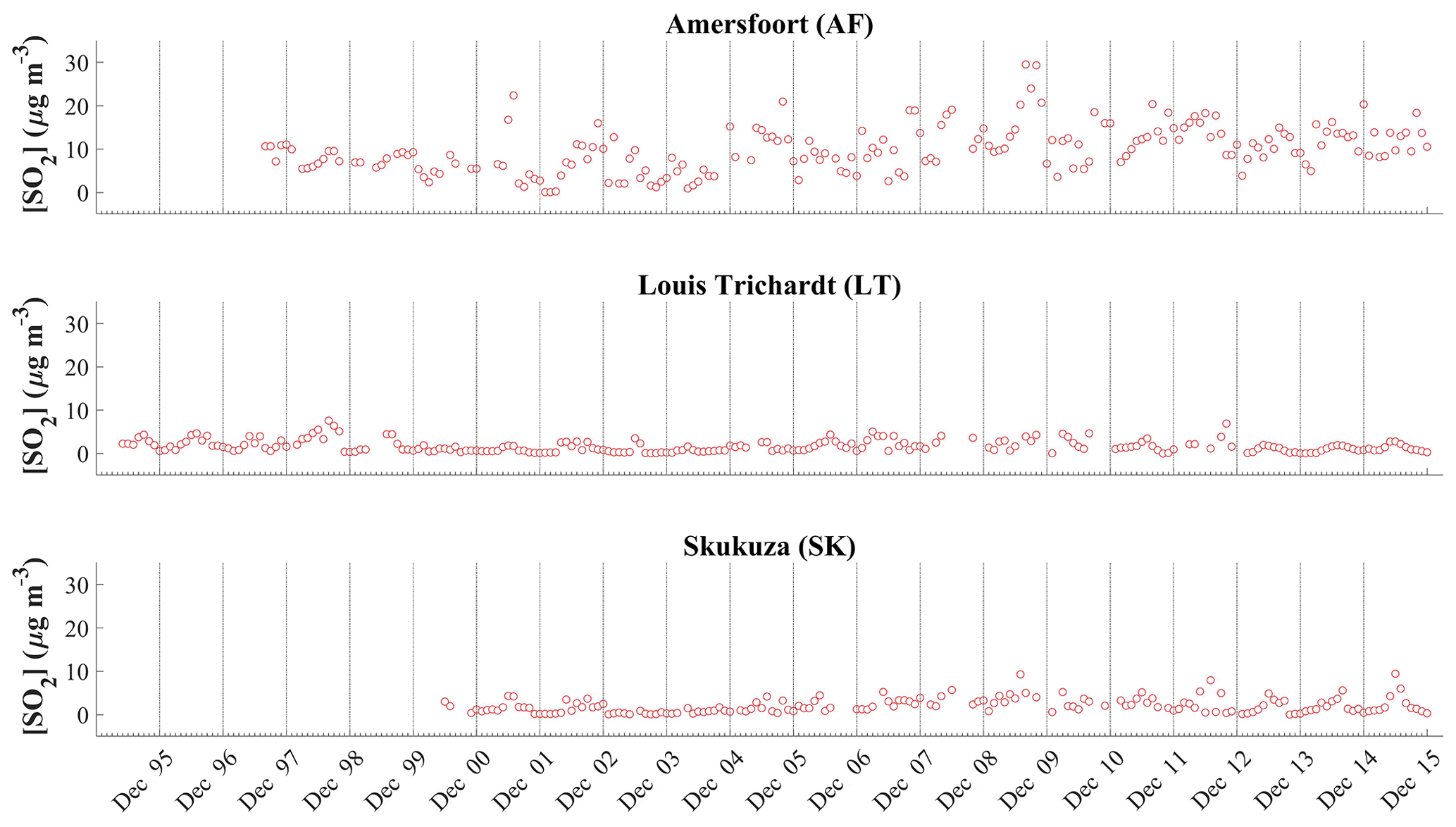
Figure A1 Time series of monthly average SO₂ concentrations measured at Amersfoort (AF), Louis Trichardt (LT) and Skukuza (SK) using passive samplers over the relevant measurement periods.

Figure A2 Time series of monthly average NO₂ concentrations measured at Amersfoort (AF), Louis Trichardt (LT) and Skukuza (SK) using passive samplers over the relevant measurement periods.

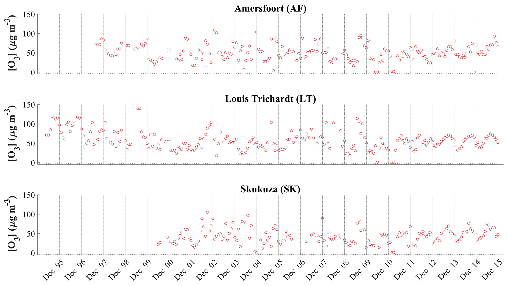
Figure A3 Time series of monthly average O₃ concentrations measured at Amersfoort (AF), Louis Trichardt (LT) and Skukuza (SK) using passive samplers over the relevant measurement periods.

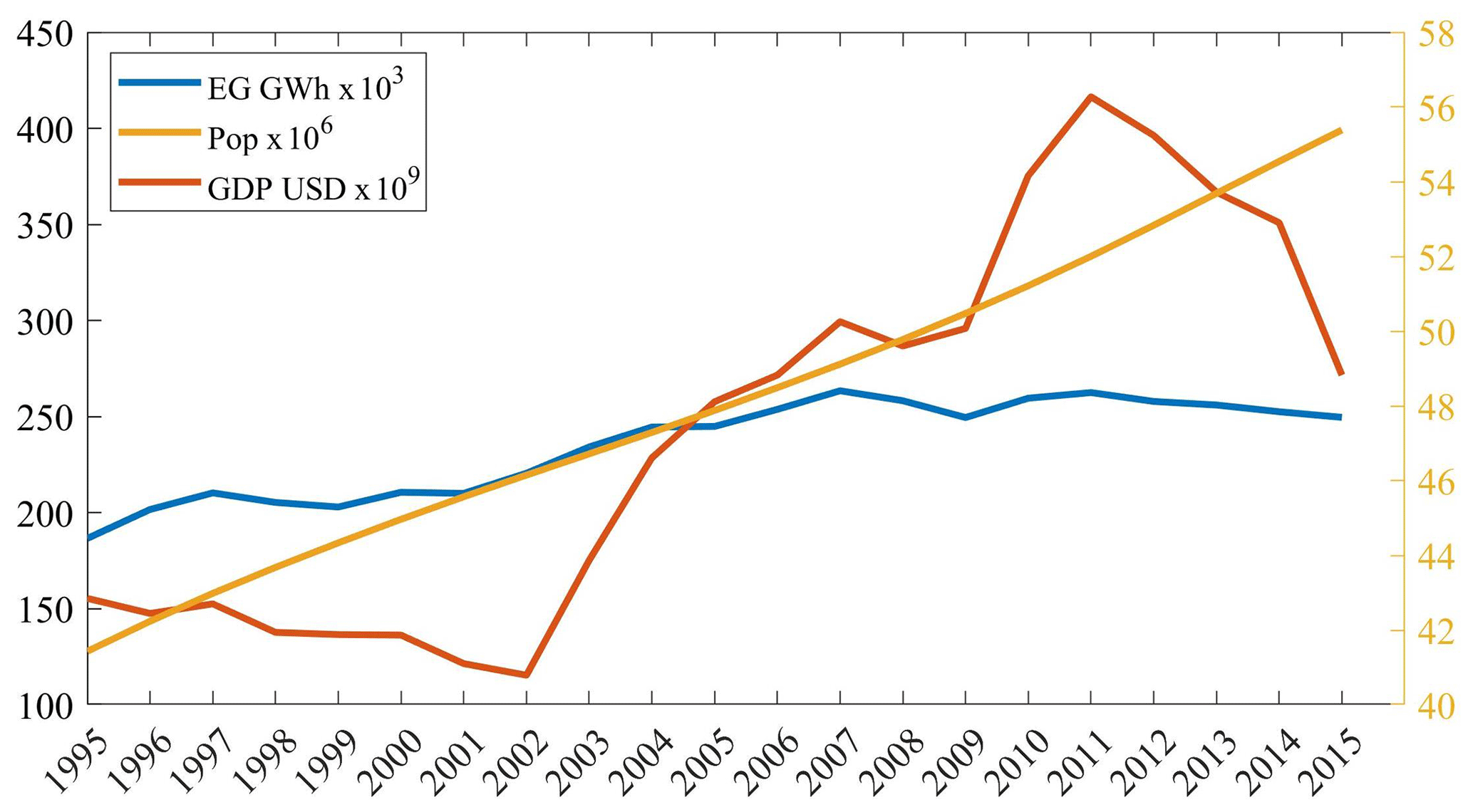
Figure A4 South African population (Pop) and GDP from 1995 to 2015 (World Bank, 2019), as well as electricity generation (EG) during this period (International Energy Agency, 2020).

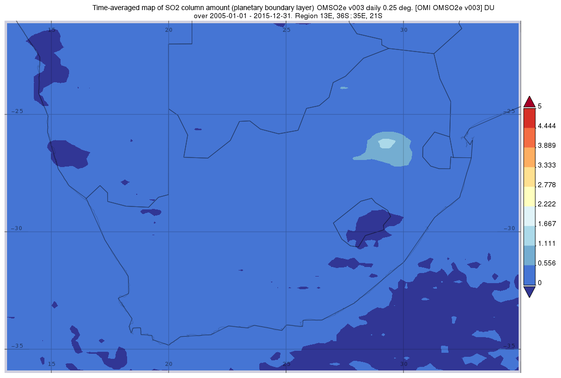
Figure A5 Geospatial map of southern Africa depicting the SO₂ column amount averaged over the period 2005 to 2015 obtained using the data from the NASA Giovanni satellite (https://giovanni.gsfc.nasa.gov/giovanni/, last access: 20 June 2019). OMI: Aura Ozone Monitoring Instrument. OMSO2e v003: OMI Level-3e SO₂ Data Product. DU: Dobson unit.

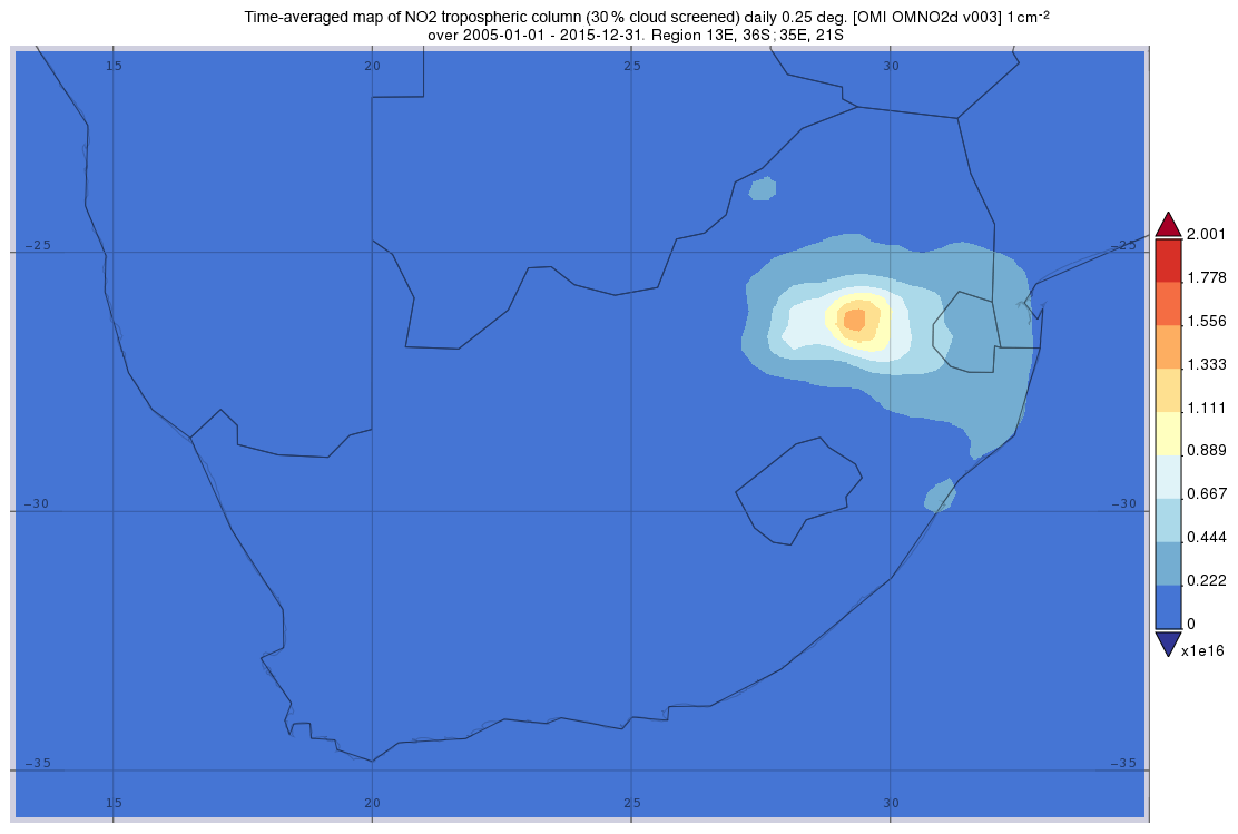
Figure A6 Geospatial map of southern Africa depicting the NO₂ tropospheric column density averaged over the period 2005 to 2015 obtained using the data from the NASA Giovanni satellite (https://giovanni.gsfc.nasa.gov/giovanni/). OMI: Aura Ozone Monitoring Instrument. OMSO2e v003: OMI Level-3e SO₂ Data Product. DU: Dobson unit.