Chlorine partitioning near the polar vortex edge observed with ground-based FTIR and satellites at Syowa Station, Antarctica, in 2007 and 2011

We retrieved lower stratospheric vertical profiles of O₃, HNO₃, and HCl from solar spectra taken with a ground-based Fourier transform infrared spectrometer (FTIR) installed at Syowa Station, Antarctica (69.0^∘ S, 39.6^∘ E), from March to December 2007 and September to November 2011. This was the first continuous measurement of chlorine species throughout the ozone hole period from the ground in Antarctica. We analyzed temporal variation of these species combined with ClO, HCl, and HNO₃ data taken with the Aura MLS (Microwave Limb Sounder) satellite sensor and ClONO₂ data taken with the Envisat MIPAS (the Michelson Interferometer for Passive Atmospheric Sounding) satellite sensor at 18 and 22 km over Syowa Station. An HCl and ClONO₂ decrease occurred from the end of May at both 18 and 22 km, and eventually, in early winter, both HCl and ClONO₂ were almost depleted. When the sun returned to Antarctica in spring, enhancement of ClO and gradual O₃ destruction were observed. During the ClO-enhanced period, a negative correlation between ClO and ClONO₂ was observed in the time series of the data at Syowa Station. This negative correlation was associated with the relative distance between Syowa Station and the edge of the polar vortex. We used MIROC3.2 chemistry–climate model (CCM) results to investigate the behavior of whole chlorine and related species inside the polar vortex and the boundary region in more detail. From CCM model results, the rapid conversion of chlorine reservoir species (HCl and ClONO₂) into Cl₂, gradual conversion of Cl₂ into Cl₂O₂, increase in HOCl in the winter period, increase in ClO when sunlight became available, and conversion of ClO into HCl were successfully reproduced. The HCl decrease in the winter polar vortex core continued to occur due to both transport of ClONO₂ from the subpolar region to higher latitudes, providing a flux of ClONO₂ from more sunlit latitudes into the polar vortex, and the heterogeneous reaction of HCl with HOCl. The temporal variation of chlorine species over Syowa Station was affected by both heterogeneous chemistries related to polar stratospheric cloud (PSC) occurrence inside the polar vortex and transport of a NO_x-rich air mass from the polar vortex boundary region, which can produce additional ClONO₂ by reaction of ClO with NO₂. The deactivation pathways from active chlorine into reservoir species (HCl and/or ClONO₂) were confirmed to be highly dependent on the availability of ambient O₃. At 18 km, where most ozone was depleted, most ClO was converted to HCl. At 22 km where some O₃ was available, an additional increase in ClONO₂ from the prewinter value occurred, similar to the Arctic.

1 Introduction

Discussion of the detection of the recovery of the Antarctic ozone hole as the result of chlorofluorocarbon (CFC) regulations has been attracting attention. The occurrence of the Antarctic ozone hole is predicted to continue at least until the middle of this century. The world's leading chemistry–climate models (CCMs) indicate that the multimodel mean time series of the springtime Antarctic total column ozone will return to 1980 levels shortly after the midcentury (about 2060) (WMO, 2019). In fact, the recovery time predicted by CCMs has a large uncertainty, and the observed ozone hole magnitude also shows year-to-year variability (e.g., see Figs. 4–6 in WMO, 2019). Although Solomon et al. (2016) and de Laat et al. (2017) reported signs of healing in the Antarctic ozone layer only in September, there is no statistically conclusive report on the Antarctic ozone hole recovery (Yang et al., 2008; Kuttippurath et al., 2010; WMO, 2019).

To understand ozone depletion processes in polar regions, understanding the behavior and partitioning of active chlorines (${\mathrm{ClO}}_x=\mathrm{Cl}+{\mathrm{Cl}}_{\mathrm{2}}+\mathrm{ClO}+\mathrm{ClOO}+{\mathrm{Cl}}_{\mathrm{2}}{\mathrm{O}}_{\mathrm{2}}$) and chlorine reservoirs (HCl and ClONO₂) is crucial. Recently, the importance of ClONO₂ was reviewed by von Clarmann and Johansson (2018). The chlorine reservoir is converted to active chlorine that destroys ozone on polar stratospheric clouds (PSCs) and/or cold binary sulfate through heterogeneous reactions:

$$\begin{array}{}\text{(R1)}& {\displaystyle }{\mathrm{ClONO}}_{\mathrm{2}}\left(\mathrm{g}\right)+\mathrm{HCl}(\mathrm{s},\mathrm{l})\to {\mathrm{Cl}}_{\mathrm{2}}\left(\mathrm{g}\right)+{\mathrm{HNO}}_{\mathrm{3}},\text{(R2)}& {\displaystyle }{\mathrm{ClONO}}_{\mathrm{2}}\left(\mathrm{g}\right)+{\mathrm{H}}_{\mathrm{2}}\mathrm{O}(\mathrm{s},\mathrm{l})\to \mathrm{HOCl}\left(\mathrm{g}\right)+{\mathrm{HNO}}_{\mathrm{3}},\end{array}$$

where g, s, and l represent the gas, solid, and liquid phases, respectively (Solomon et al., 1986; Solomon, 1999; Drdla and Müller, 2012; Wegner et al., 2012; Nakajima et al., 2016).

Heterogeneous reactions,

$$\begin{array}{}\text{(R3)}& {\displaystyle }{\mathrm{N}}_{\mathrm{2}}{\mathrm{O}}_{\mathrm{5}}\left(\mathrm{g}\right)+\mathrm{HCl}(\mathrm{s},\mathrm{l})\to {\mathrm{ClNO}}_{\mathrm{2}}\left(\mathrm{g}\right)+{\mathrm{HNO}}_{\mathrm{3}},\text{(R4)}& {\displaystyle }\mathrm{HOCl}\left(\mathrm{g}\right)+\mathrm{HCl}(\mathrm{s},\mathrm{l})\to {\mathrm{Cl}}_{\mathrm{2}}\left(\mathrm{g}\right)+{\mathrm{H}}_{\mathrm{2}}\mathrm{O},\end{array}$$

are responsible for additional chlorine activation. When solar illumination is available, Cl₂, HOCl, and ClNO₂ are photolyzed to produce chlorine atoms by reactions

$$\begin{array}{}\text{(R5)}& {\displaystyle }{\mathrm{Cl}}_{\mathrm{2}}+h\mathit{\nu }\to \mathrm{Cl}+\mathrm{Cl},\text{(R6)}& {\displaystyle }\mathrm{HOCl}+h\mathit{\nu }\to \mathrm{Cl}+\mathrm{OH},\text{(R7)}& {\displaystyle }{\mathrm{ClNO}}_{\mathrm{2}}+h\mathit{\nu }\to \mathrm{Cl}+{\mathrm{NO}}_{\mathrm{2}}.\end{array}$$

The yielded chlorine atoms then start to destroy ozone catalytically through reactions (Canty et al., 2016):

$$\begin{array}{}\text{(R8)}& {\displaystyle }\mathrm{Cl}+{\mathrm{O}}_{\mathrm{3}}\to \mathrm{ClO}+{\mathrm{O}}_{\mathrm{2}},\text{(R9)}& {\displaystyle }\mathrm{ClO}+\mathrm{ClO}+M\to {\mathrm{Cl}}_{\mathrm{2}}{\mathrm{O}}_{\mathrm{2}}+M,\text{(R10)}& {\displaystyle }{\mathrm{Cl}}_{\mathrm{2}}{\mathrm{O}}_{\mathrm{2}}+h\mathit{\nu }\to \mathrm{Cl}+\mathrm{ClOO},\text{(R11)}& {\displaystyle }\mathrm{ClOO}+M\to \mathrm{Cl}+{\mathrm{O}}_{\mathrm{2}}+M.\end{array}$$

There are three types of PSCs, i.e., nitric acid trihydrate (NAT), supercooled ternary solution (STS), and ice PSCs. When the stratospheric temperatures get warmer than NAT saturation temperature (about 195 K at 50 hPa) and no PSCs are present, deactivation of chlorine starts to occur. Reformation of ClONO₂ and HCl mainly occurs through reactions (Santee et al., 2008; Grooß et al., 2011; Müller et al., 2018)

$$\begin{array}{}\text{(R12)}& {\displaystyle }\mathrm{ClO}+{\mathrm{NO}}_{\mathrm{2}}+M\to {\mathrm{ClONO}}_{\mathrm{2}}+M,\text{(R13)}& {\displaystyle }\mathrm{Cl}+{\mathrm{CH}}_{\mathrm{4}}\to \mathrm{HCl}+{\mathrm{CH}}_{\mathrm{3}},\text{(R14)}& {\displaystyle }{\mathrm{CH}}_{\mathrm{2}}\mathrm{O}+\mathrm{Cl}\to \mathrm{HCl}+\mathrm{CHO}.\end{array}$$

The reformation of ClONO₂ by Reaction (R12) from active chlorine is much faster than that of HCl by Reactions (R13) and (R14) if enough NO_x are available (Mellqvist et al., 2002; Dufour et al., 2006). But the formation rates of ClONO₂ and HCl are also related to ozone concentration. Grooß et al. (1997) showed that HCl increases more rapidly in the Antarctic polar vortex than in the Arctic polar vortex due to lower ozone concentrations in the Antarctic polar vortex. Low ozone reduces the rate of Reaction (R8) and then the Cl∕ClO ratio increases. Low ozone also reduces the rate of the following reaction:

$$\begin{array}{}\text{(R15)}& \mathrm{NO}+{\mathrm{O}}_{\mathrm{3}}\to {\mathrm{NO}}_{\mathrm{2}}+{\mathrm{O}}_{\mathrm{2}}.\end{array}$$

This makes the NO∕NO₂ ratio high and increases the Cl∕ClO ratio using the following reaction:

$$\begin{array}{}\text{(R16)}& \mathrm{ClO}+\mathrm{NO}\to \mathrm{Cl}+{\mathrm{NO}}_{\mathrm{2}}.\end{array}$$

A high Cl∕ClO ratio leads to rapid HCl formation by Reactions (R13) and (R14) and reduces the formation ratio of ClONO₂ by Reaction (R12) (Grooß et al., 2011; Müller et al., 2018).

The processes of deactivation of active chlorine are different between typical conditions in the Antarctic and those in the Arctic. In the Antarctic, the temperature cools below the NAT PSC existence threshold (about 195 K at 50 hPa) in the whole area of the polar vortex in all years, and almost complete denitrification and chlorine activation occur (WMO, 2007), followed by severe ozone depletion in spring. In the chlorine reservoir recovery phase, HCl is mainly formed by Reaction (R13) due to the lack of ozone (typically less than 0.5 ppmv) using the mechanism described in the previous paragraph (Grooß et al., 2011).

On the other hand, in the Arctic, typically less PSC formation occurs in the polar vortex due to generally higher stratospheric temperatures (∼ 10–15 K on average) compared with that of Antarctica. Then only partial denitrification and chlorine activation occur in some years (Manney et al., 2011; WMO, 2014). In this case, some ozone and NO₂ are available in the chlorine reservoir recovery phase. Therefore, the ClONO₂ amount becomes higher than that of HCl after PSCs have disappeared due to the rapid Reaction (R12) (Michelsen et al., 1999; Santee et al., 2003), which results in an additional increase in ClONO₂ than the prewinter value at the time of chlorine deactivation in spring (von Clarmann et al., 1993; Müller et al., 1994; Oelhaf et al., 1994). In this way, the partitioning of the chlorine reservoir in springtime is related to temperature, PSC amounts, ozone, and NO₂ concentrations (Santee et al., 2008; Solomon et al., 2015).

In the polar regions, the ozone and related atmospheric trace gas species have been intensively monitored by several measurement techniques since the discovery of the ozone hole. These measurements consist of direct observations by high-altitude aircraft (e.g., Anderson et al., 1989; Ko et al., 1989; Tuck et al., 1995; Jaeglé et al., 1997; Bonne et al., 2000), remote-sensing observations by satellites (e.g., Müller et al., 1996; Michelsen et al., 1999; Höpfner et al., 2004; Dufour et al., 2006; Hayashida et al., 2007), remote-sensing observations of OClO using a UV–visible spectrometer from the ground (Solomon et al., 1987; Kreher et al., 1996), and remote-sensing observations of ClO by a microwave spectrometer from the ground (de Zafra et al., 1989). Within these observations, ground-based measurements have the characteristic of high temporal resolution. In addition, the Fourier transform infrared spectrometer (FTIR) has the capability of measuring several trace gas species at the same time or in a short time interval (Rinsland et al., 1988). In this paper, we show the results of ground-based FTIR observations of O₃ and other trace gas species at Syowa Station in the Antarctic in 2007 and 2011, combined with satellite measurements of trace gas species from the Microwave Limb Sounder on board the Aura satellite (Aura MLS) and Michelson Interferometer for Passive Atmospheric Sounding on board the European Environmental Satellite (Envisat MIPAS), to show the temporal variation and partitioning of active chlorine (ClO_x) and chlorine reservoirs (HCl, ClONO₂) from fall to spring during the ozone hole formation and dissipation period. In order to monitor the appearance of PSCs over Syowa Station, we used the Cloud-Aerosol Lidar with Orthogonal Polarization (CALIOP) data on board the Cloud-Aerosol Lidar and Infrared Pathfinder Satellite Observations (CALIPSO) satellite. The methods of FTIR and satellite measurements are described in Sect. 2. The validation of FTIR measurements is described in Sect. 3. The results of FTIR and satellite measurements and discussion on the behavior of active and inert chlorine species using the MIROC3.2 chemistry–climate model are described in Sect. 4.

2 Measurements

2.1 FTIR measurements

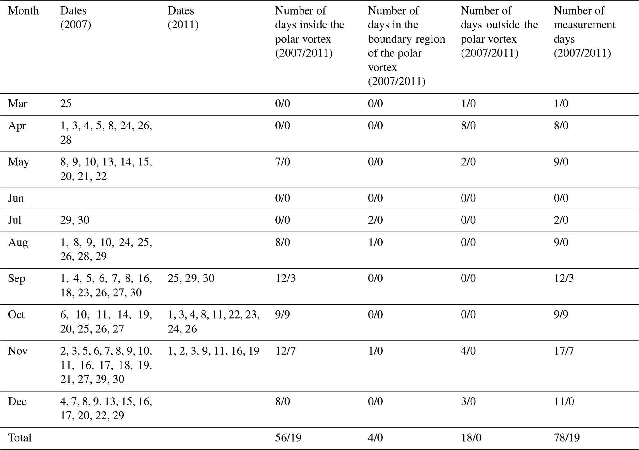
The Japanese Antarctic Syowa Station (69.0^∘ S, 39.6^∘ E) was established in January 1957. Since then, several scientific observations related to meteorology, upper atmospheric physics, glaciology, biology, geology, seismology, etc. have been performed. The ozone hole was first detected by Dobson spectrometer and ozonesonde measurements from Syowa Station in 1982 (Chubachi, 1984) and by Dobson spectrometer measurements at Halley Bay (Farman et al., 1985). We installed a Bruker IFS-120M high-resolution Fourier transform infrared spectrometer (FTIR) in the observation hut at Syowa Station in March 2007. This was the third high-resolution FTIR site in Antarctica in operation after the USA's South Pole Station (90.0^∘ S) (Goldman et al., 1983, 1987; Murcray et al., 1987), the USA's McMurdo Station, and New Zealand's Arrival Heights facility at the Scott Base station (77.8^∘ S, 166.7^∘ E) (Farmer et al., 1987; Murcray et al., 1989; Kreher et al., 1996; Wood et al., 2002, 2004). The IFS-120M FTIR has a wavenumber resolution of 0.0035 cm⁻¹, with two liquid-nitrogen-cooled detectors (with InSb and HgCdTe covering the frequency ranges 2000–5000 and 700–1300 cm⁻¹, respectively) with six optical filters, and is fed by an external solar tracking system. One measurement takes about 10 min. At least six spectra were taken per day, covering each filter region. Since Syowa Station is located at a relatively low latitude (69.0^∘ S) compared with McMurdo or Scott Base stations (77.8^∘ S), there is an advantage of the short (about 1 month) polar night period, when we cannot measure atmospheric species using the sun as a light source. Since FTIR measurements at Syowa Station are possible from early spring (late July), FTIR can measure chemical species during ozone hole development. On the other hand, FTIR observations become possible only after September at McMurdo and Scott Base stations. Another advantage of Syowa Station is that it is sometimes located at the vortex boundary as well as inside and outside of the polar vortex, and this enables us to measure chemical species at different regions of polar chemistry related to the ozone hole. From March to December 2007, we made in total 78 d of FTIR measurements on sunny days. Another 19 d of FTIR measurements were performed from September to November 2011. After a few more measurements were performed in 2016, the FTIR was brought back to Japan in 2017. In Appendix A, Table A1 shows the days when FTIR measurements were made at Syowa Station with the information inside, in the boundary region, and outside of the polar vortex defined by the method described in Appendix B using ERA-Interim reanalysis data. Strahan et al. (2014) showed the year-to-year variation of Cl_y observed in the lower stratosphere of the Antarctic polar vortex. The Cl_y observed in 2007 (2.88 ppbv) was about +4.3 % more and that observed in 2011 (2.53 ppbv) was about −5.2 % less than the projected Cl_y from Newman et al. (2007) (2.76 ppbv for 2007 and 2.67 ppbv for 2011).

The retrieval of the FTIR spectra was done with the SFIT2 version 3.92 program (Rinsland et al., 1998; Hase et al., 2004). SFIT2 retrieves a vertical profile of trace gases using an optimal estimation formulation of Rodgers (2000), implemented with a semiempirical method which was originally developed for microwave measurements (Parrish et al., 1992; Connor et al., 1995). The SFIT2 forward model fully describes the FTIR instrument response, with absorption coefficients calculated using the algorithm of Norton and Rinsland (1991). The atmosphere is constructed with 47 layers from the ground to 100 km, using the FSCATM (Gallery et al., 1983) program for atmospheric ray tracing to account for refractive bending. The retrieval parameters for each gas, typical vertical resolution, and typical mean degrees of freedom for signal (DOFS) are shown in Table 1. Temperature and pressure profiles between 0 and 30 km are taken by the rawinsonde observations flown from Syowa Station on the same day by the Japanese Meteorological Agency (JMA), while values between 30 and 100 km are taken from the COSPAR International Reference Atmosphere 1986 (CIRA-86) standard atmosphere profile (Rees et al., 1990).

Table 1 Retrieval parameters of SFIT2.

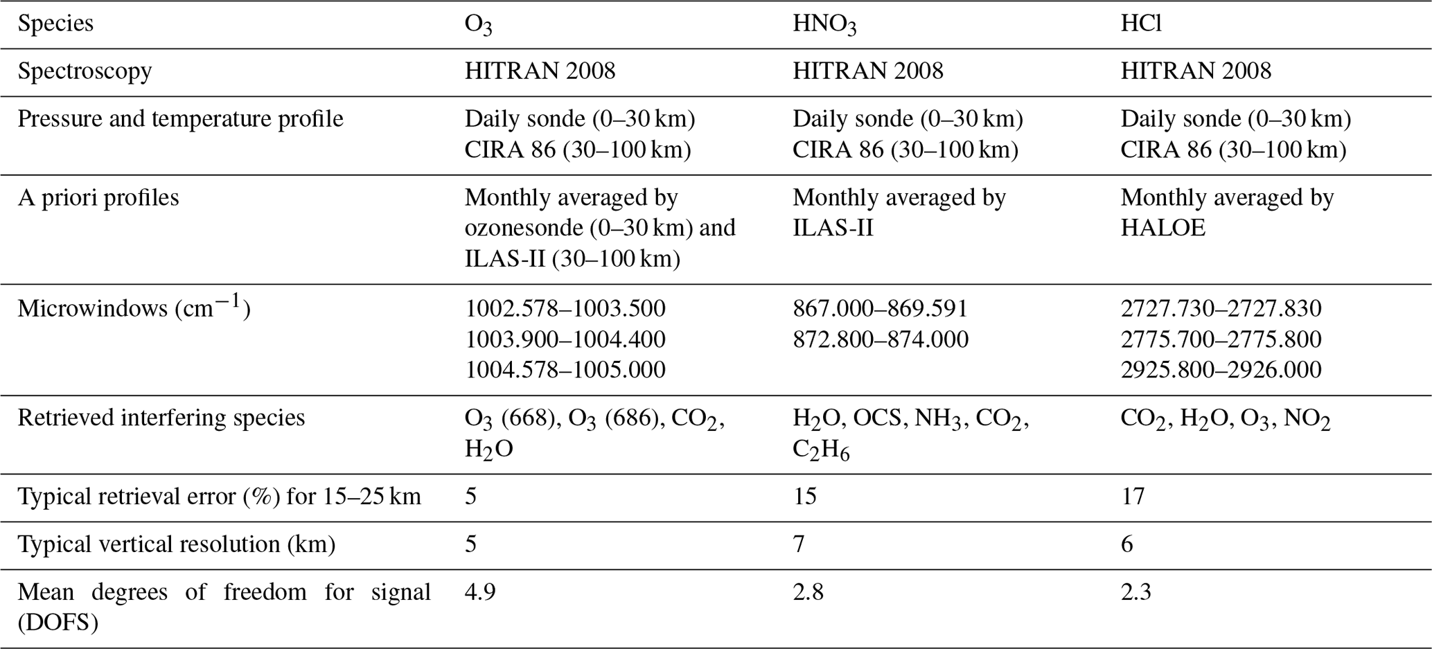
We retrieved vertical profiles of O₃, HCl, and HNO₃ from the solar spectra. We used monthly averaged ozonesondes profiles (0–30 km) and Improved Limb Atmospheric Spectrometer-II (ILAS-II) (Nakajima, 2006; Nakajima et al., 2006; Sugita et al., 2006) profiles (30–100 km) for the a priori profiles of O₃, monthly averaged profiles from ILAS-II for HNO₃, and monthly averaged profiles from HALOE (Anderson et al., 2000) for HCl. We focus on the altitude range of 15–25 km in this study. Typical averaging kernels of the SFIT2 retrievals for O₃, HNO₃, and HCl are shown in Fig. 1a, b, and c, respectively.

Figure 1 Averaging kernel functions of the SFIT2 retrievals for (a) O₃, (b) HNO₃, and (c) HCl.

2.2 Satellite measurements

The Earth Observing System (EOS) MLS on board the Aura satellite was launched on 15 July 2004 to monitor several atmospheric chemical species in the upper troposphere to mesosphere (Waters et al., 2006). The Aura orbit is sun-synchronous at 705 km altitude, with an inclination of 98^∘, 13:45 ascending (north-going) Equator-crossing time, and 98.8 min period. Vertical profiles are measured every ∼165 km along the suborbital track, the horizontal resolution is ∼ 200–600 km along track and ∼ 3–10 km across track, and the vertical resolution is ∼ 3–4 km in the lower-to-middle stratosphere (Froidevaux et al., 2006). ClO, HCl, and HNO₃ profiles used in this study were taken from Aura MLS version 4.2 data (Livesey et al., 2006, 2018; Santee et al., 2011; Ziemke et al., 2011). Only daytime ClO data were used for the analysis. The daily MLS data within 320 km distance between the measurement location and Syowa Station were selected.

MIPAS is a Fourier transform spectrometer sounding the thermal emission of the earth's atmosphere between 685 and 2410 cm⁻¹ (14.6–4.15 µm) in limb geometry (Fischer and Oelhaf, 1996; Fischer et al., 2008). The maximum optical path difference of MIPAS is 20 cm. The field of view of the instrument at the tangent points is about 3 km in the vertical and 30 km in the horizontal. In the standard observation mode in one limb scan, 17 tangent points are observed with nominal altitudes 6, 9, 12, 15, 18, 21, 24, 27, 30, 33, 36, 39, 42, 47, 52, 60, and 68 km. In this mode, about 73 limb scans are recorded per orbit. The measurements of each orbit cover nearly the complete latitude range from about 87^∘ S to 89^∘ N. MIPAS was placed on board Envisat, which was launched on 1 March 2002, and was put into a polar sun-synchronous orbit at an altitude of about 800 km with an inclination of 98.55^∘ (von Clarmann et al., 2003). On its descending node, the satellite crosses the Equator at 10:00 local time. Envisat performs 14.3 orbits per day, which results in a good global coverage. The ClONO₂ profiles which we used in this study were taken from Envisat MIPAS IMK/IAA version V5R_CLONO2_220 and V5R_CLONO2_222 (Höpfner et al., 2007). The daily MIPAS data within 320 km distance between the measurement location and Syowa Station were selected.

The CALIPSO satellite was launched on 28 April 2006. On the CALIPSO satellite, the CALIOP instrument was on board to monitor aerosols, clouds, and PSCs (Pitts et al., 2007). CALIOP is a two-wavelength, polarization-sensitive lidar that provides high-vertical-resolution profiles of the backscatter coefficient at 532 and 1064 nm, as well as two orthogonal (parallel and perpendicular) polarization components at 532 nm (Winker et al., 2007). In order to monitor the appearance of PSCs over Syowa Station, the daily CALIOP PSC data (Pitts et al., 2007, 2009, 2011) within 320 km distance between the measurement location and Syowa Station were selected.

3 Validation of retrieved profiles from FTIR spectra with other measurements

We validated retrieved FTIR profiles of O₃ with ozonesondes and Aura MLS version 3.3 data (Livesey et al., 2013) for 2007 measurements. Also, retrieved FTIR profiles of HNO₃ and HCl were validated with Aura MLS data. We identified the nearest Aura MLS data from the distance between the Aura MLS tangent point and the point for the direction of the sun from Syowa Station at the time of the FTIR measurement at 20 km. The spatial and temporal collocation criteria used were within a 300 km radius and ±6 h. The ozonesonde and Aura MLS profiles were interpolated onto a 1 km grid and then smoothed using a 5 km wide running mean.

Figure 2a–b show absolute and relative differences of O₃ profiles retrieved from FTIR measurements and those from model 1Z ECC-type ozonesonde measurements, respectively, calculated from 14 coincident measurements from 5 September to 17 December 2007. The typical precision and accuracy of the ECC-type ozone sondes are considered to be ± (3–5) % and ± (4–5) %, respectively (Komhyr, 1986). We define the relative percentage difference D as

$$\begin{array}{}\text{(1)}& D\left(\mathit{\%}\right)=\mathrm{100}\cdot (\mathrm{FTIR}-\mathrm{sonde})/\left(\right(\mathrm{FTIR}+\mathrm{sonde})/\mathrm{2}).\end{array}$$

The mean absolute difference between 15 and 25 km was within −0.02 to 0.40 ppmv. The mean relative difference D between 15 and 25 km was within −10.4 % to +24.4 %. The average of the mean relative differences D of O₃ for the altitude of interest in this study (18–22 km) was +6.1 %, with the minimum of −10.4 % and the maximum of +19.2 %. FTIR data agree with validation data within root mean squares of typical errors in FTIR and validation data at the altitude of interest. Note that relatively large D values between 16 and 18 km are due to the small ozone amount in the ozone hole. Our validation results are quite comparable with the validation study at Izaña Observatory by Schneider et al. (2008).

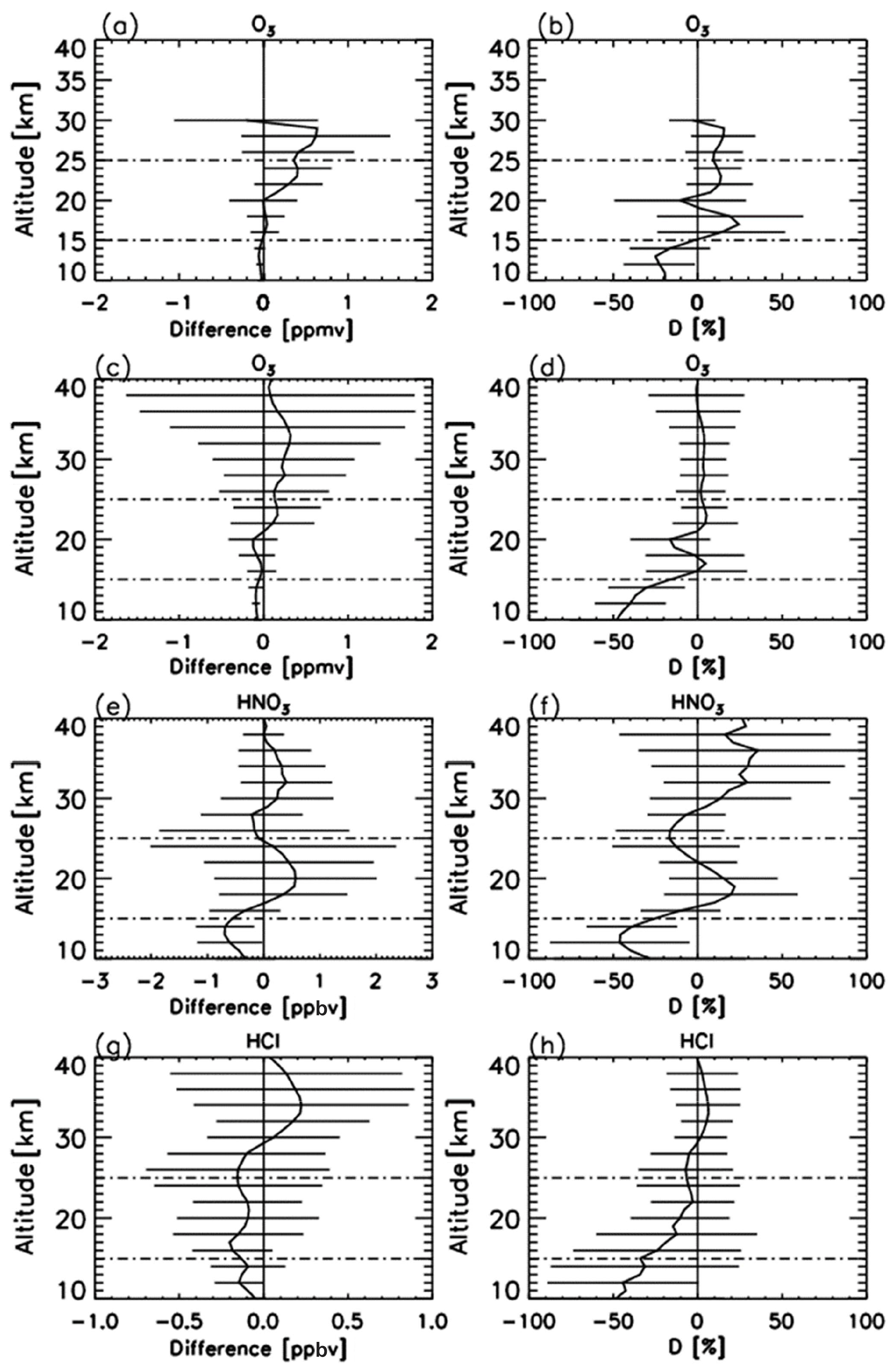
Figure 2 (a) Mean absolute and (b) mean relative differences of O₃ profiles retrieved from FTIR measurements minus those from ozonesonde measurements. (c) Mean absolute and (d) mean relative differences of O₃ profiles retrieved from FTIR measurements minus those from Aura MLS measurements. (e) Mean absolute and (f) mean relative differences of HNO₃ profiles retrieved from FTIR measurements minus those from Aura MLS measurements. (g) Mean absolute and (h) mean relative differences of HCl profiles retrieved from FTIR measurements minus those from Aura MLS measurements. Horizontal bars indicate the root mean squares of differences at each altitude. Horizontal dashed bars indicate the altitude range of our focus (15–25 km).

Figure 2c–d show absolute and relative differences of O₃ profiles retrieved from FTIR measurements and those from Aura MLS measurements, respectively, calculated from 33 coincident measurements from 1 April to 20 December 2007. The accuracy of MLS O₃ data is reported to be 5 %–8 % between 0.5 and 46 hPa (Livesey et al., 2013). The mean absolute difference between 15 and 25 km was within −0.13 to +0.16 ppmv. The mean relative difference D between 15 and 25 km was within −16.2 % to +5.2 %. The average of the mean relative differences D for O₃ for the altitude of interest in this study (18–22 km) was −5.5 %, with the minimum of −16.3 % and the maximum of +4.5%. Froidevaux et al. (2008) showed that Aura MLS is +8 % higher than the Atmospheric Chemistry Experiment Fourier transform spectrometer (ACE-FTS) at 70^∘ S, which may explain the negative bias of FTIR data compared with MLS data.

Figure 2e–f show absolute and relative differences of HNO₃ profiles retrieved by FTIR measurements and those from Aura MLS measurements, respectively, calculated from 47 coincident measurements from 25 March to 20 December 2007. The mean absolute difference between 15 and 25 km was within −0.56 to +0.57 ppbv. The mean relative difference D between 15 and 25 km was within −25.5 % to +21.9 %. The average of the mean relative differences D for HNO₃ for the altitude of interest in this study (18–22 km) was +13.2 %, with the minimum of +0.2 % and the maximum of +21.9 %. This positive bias of FTIR data is still within the error bars of FTIR measurements. Livesey et al. (2013) showed that Aura MLS version 3.3 data have no bias within errors (∼ 0.6–0.7 ppbv (10 %–12 %) at a pressure level of 100–3.2 hPa) compared with other measurements. Livesey et al. (2018) showed no major differences between Aura MLS version 3.3 and version 4.2 data for HNO₃.

Figure 2g–h show absolute and relative differences of HCl profiles retrieved by FTIR measurements and those from Aura MLS measurements, respectively, calculated from 50 coincident measurements from 25 March to 20 December 2007. The mean absolute difference between 15 and 25 km was within −0.20 to −0.09 ppbv. The mean relative difference D between 15 and 25 km was within −34.1 % to −3.0 %. The average of mean relative differences D for HCl for the altitude of interest in this study (18–22 km) is −9.7 %, with a minimum of −14.6 % and a maximum of −3.0 %. This negative bias of FTIR data is still within the error bars of FTIR measurements. Moreover, Livesey et al. (2013) showed that Aura MLS version 3.3 values are systematically greater than HALOE values by 10 %–15 % with a precision of 0.2–0.6 ppbv (10 %–30 %) in the stratosphere, which may partly explain the negative bias of FTIR data compared with MLS data. Livesey et al. (2018) showed no major differences between Aura MLS version 3.3 and version 4.2 data for HCl.

Table 2 summarizes the validation results of FTIR profiles compared with ozonesonde or Aura MLS measurements, as well as possible Aura MLS biases from the literature.

Table 2 Summary of validation results of FTIR profiles compared with ozonesonde and Aura MLS measurements, as well as possible Aura MLS biases from the literature.

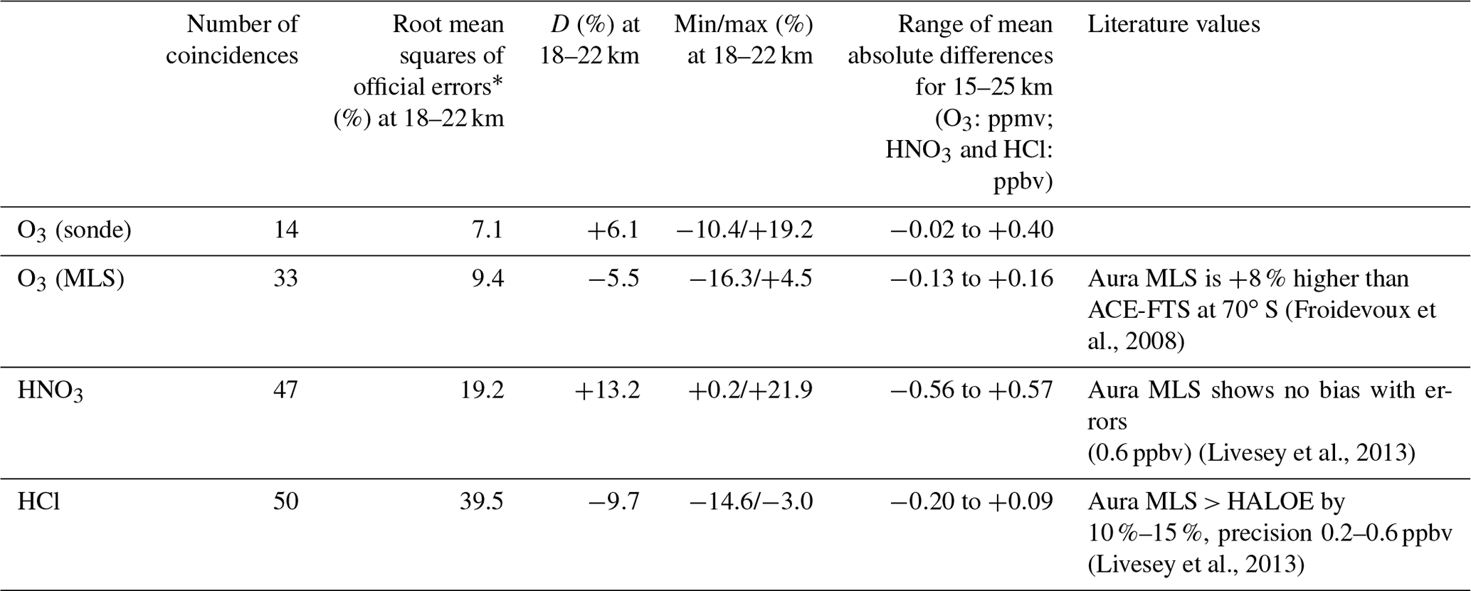
^* Root mean squares of official absolute and relative errors given by each data set.

4 Results and discussion

4.1 Time series of observed species

Figure 3a shows daytime hours at Syowa Station. Polar night ends at Syowa Station on 14 July (day 195). Figure 3b–e show the time series of temperatures at 18 and 22 km over Syowa Station using ERA-Interim data (Dee et al., 2011) for 2007 and 2011. Approximate saturation temperatures for NAT (T_NAT) and ice (T_ICE) calculated by assuming 6 ppbv HNO₃ and 4.5 ppmv H₂O are also shown in the figures. The dates when PSCs were observed at Syowa Station identified by the nearest CALIOP data of that day were indicated by asterisks at the bottom of the figures. Over Syowa Station, PSCs were observed when temperature fell ∼4 K below T_NAT. PSCs were often observed at 15–25 km from the beginning of July (day 183) to late August (day 241) in 2007 and from late June (day 175) to early September (day 251) in 2011.

Figure 3 Time series of (a) daytime hour and temperatures at 18 km in (b) 2007 and (c) 2011 and at 22 km in (d) 2007 and (e) 2011 over Syowa Station using ERA-Interim data. Approximate saturation temperatures for nitric acid trihydrate (T_NAT) and ice (T_ICE) calculated by assuming 6 ppbv HNO₃ and 4.5 ppmv H₂O are also plotted in the figures by dotted lines. Dates when PSCs were observed over Syowa Station are indicated by asterisks on the bottom of the figures.

PSCs were observed only at 18 km after August, due to the sedimentation of PSCs and downwelling of vortex air in late winter as is seen in Fig. 3. Although temperatures above Syowa Station were sometimes below T_NAT-4 K in June and in late September, no PSC was observed during those periods. This may be due to other reasons, such as a different time history of temperature for PSC formation, and/or low HNO₃ (denitrification) and/or H₂O concentration (dehydration), which are needed for PSC formation in the late winter season (Saitoh et al., 2006).

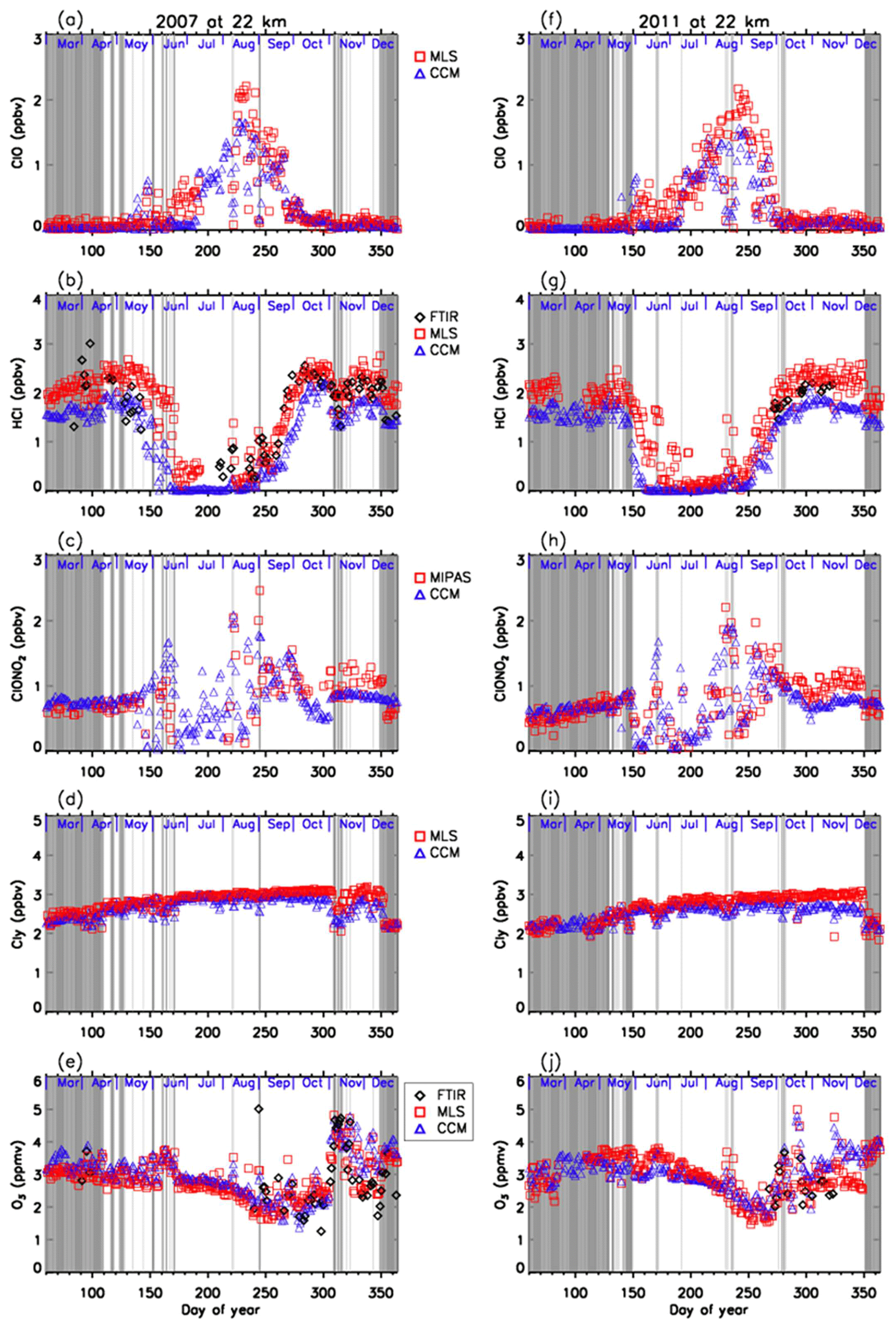
Figures 4–7 show time series of HCl, ClONO₂, ClO, ${\mathrm{Cl}}_y^{*}$, O₃, and HNO₃ over Syowa Station in 2007 and 2011 at altitudes of 18 and 22 km for all ground-based and satellite-based observations used in this study, respectively. O₃ (sonde) is observed with the KC96 ozonesonde for 2007, which is different from the ones that were used for the validation in Sect. 3 and the ECC-1Z ozonesonde for 2011 by JMA (Smit and Straeter, 2004). HCl and HNO₃ observed by Aura MLS and FTIR are plotted by different symbols. Total inorganic chlorine ${\mathrm{Cl}}_y^{*}$ corresponds to the sum of HCl, ClONO₂, and Cl_x, where the active chlorine species Cl_x is defined as the sum of ClO, Cl, and 2⋅Cl₂O₂ (Bonne et al., 2000). It is known that total inorganic chlorine ${\mathrm{Cl}}_y^{*}$ has a compact relationship with N₂O (Bonne et al., 2000; Schauffler et al., 2003; Strahan et al., 2014). Inferred total inorganic chlorine ${\mathrm{Cl}}_y^{*}$ is calculated from the N₂O value (in ppbv) measured by MLS and by using the empirical polynomial equation derived from the correlation analysis of Cl_y and N₂O from the Photochemistry of Ozone Loss in the Arctic Region in Summer (POLARIS) mission which took place from April to September 1997 (Bonne et al., 2000). In order to compensate for the temporal trends of Cl_y and N₂O values (2.90, 2.76, and 2.67 ppbv for Cl_y (Strahan et al., 2014) and 313, 321, and 324 ppbv for N₂O (WMO, 2007, 2011, 2014) for the years 1997, 2007, and 2011, respectively), we used values 8 and 11 for constant A and 140 and 230 for constant B for years 2007 and 2011 in the following equation, respectively:

$$\begin{array}{}\text{(2)}& \begin{array}{rl}{\mathrm{Cl}}_y^{*}\left(\mathrm{pptv}\right)& =\mathrm{4.7070}\times {\mathrm{10}}^{-\mathrm{7}}({\mathrm{N}}_{\mathrm{2}}\mathrm{O}-A{)}^{\mathrm{4}}\\ & -\mathrm{3.2708}\times {\mathrm{10}}^{-\mathrm{4}}({\mathrm{N}}_{\mathrm{2}}\mathrm{O}-A{)}^{\mathrm{3}}\\ & +\mathrm{4.0818}\times {\mathrm{10}}^{-\mathrm{2}}({\mathrm{N}}_{\mathrm{2}}\mathrm{O}-A{)}^{\mathrm{2}}\\ & -\mathrm{4.6856}({\mathrm{N}}_{\mathrm{2}}\mathrm{O}-A)+\mathrm{3225}-B.\end{array}\end{array}$$

A transport barrier of minor constituents at the edge of the polar vortex was reported by Lee et al. (2001) and Tilmes et al. (2006). The distribution of minor constituents is quite different among the inside, in the boundary region, and outside of the polar vortex. In Figs. 4–7, the dark shaded area, the light shaded area, and the white area indicate the days when Syowa Station was located outside, in the boundary region, and inside of the polar vortex, respectively. In the Antarctic winter, there are often double peaks in the isentropic potential vorticity (PV) gradient with respect to equivalent latitude at the 450–600 K level (Tomikawa et al., 2015). The method to determine the three polar regions, i.e., inside the polar vortex, in the boundary region of the polar vortex, and outside the polar vortex, is described in Appendix B. Note that the Syowa Station is often located near the vortex edge, and the temporal variations of chemical species observed over Syowa Station reflect the spatial distributions as well as local chemical evolution. When Syowa Station was located at the boundary region or outside the polar vortex (e.g., day 310–316 in Fig. 4, day 192–195 in Fig. 5, day 309–316 in Fig. 6, and day 276–282 in Fig. 7), chemical species showed different values compared with the ones inside the polar vortex. The lack of data for ClO and HCl (MLS) from day 195 to day 219, 2007, and ClONO₂ from day 170 to day 216, 2007 (Figs. 4a and 6a), is due to unrealistic large error values in Aura MLS or Envisat MIPAS data products during these periods.

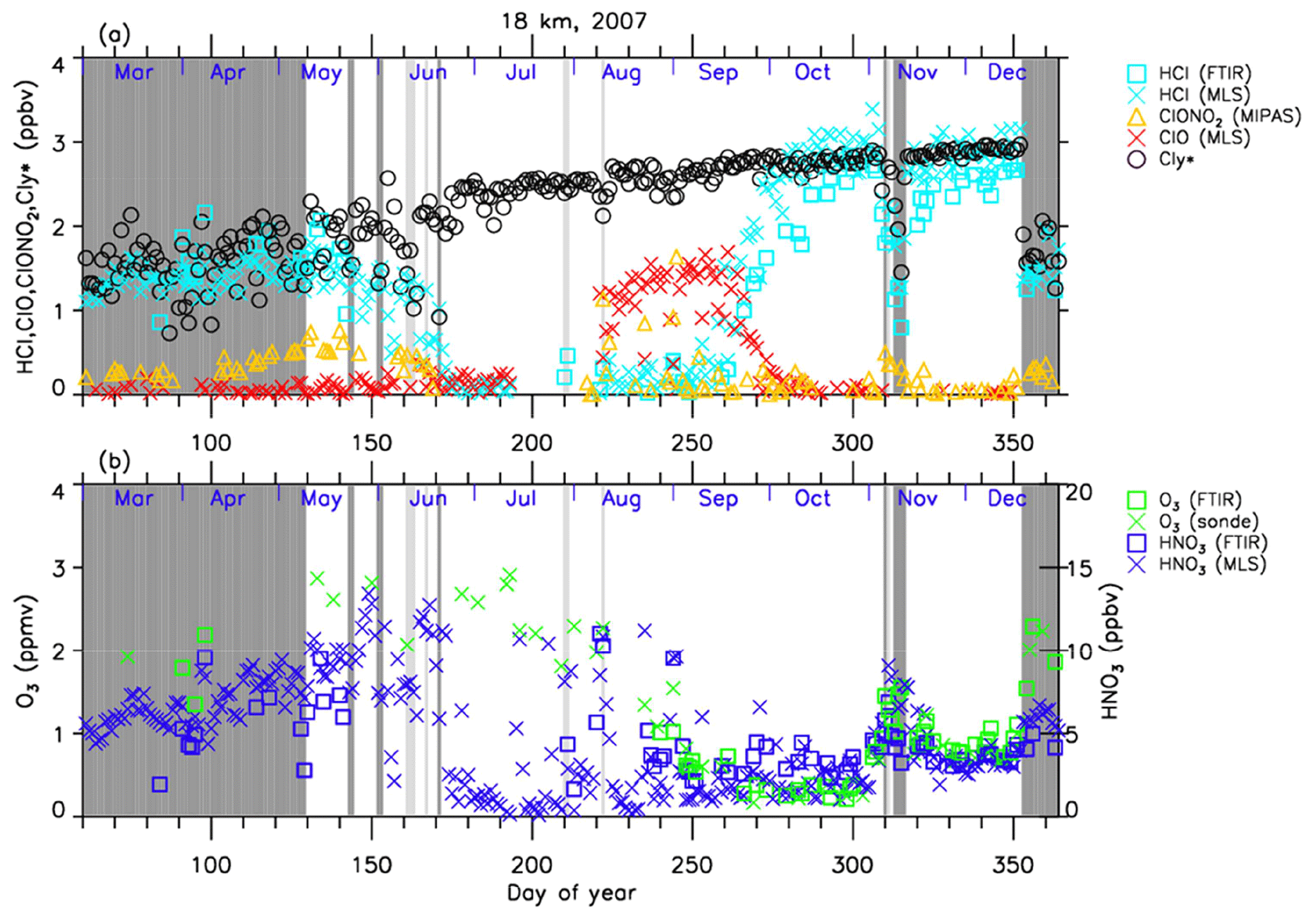
Figure 4 Time series of (a) HCl, ClONO₂, ClO, and ${\mathrm{Cl}}_y^{*}$ as well as (b) O₃ and and HNO₃ mixing ratios at 18 km in 2007 over Syowa Station. O₃(FTIR), HCl(FTIR), and HNO₃(FTIR) were measured by FTIR at Syowa Station, while HCl(MLS), ClO(MLS), and HNO₃(MLS) were measured by Aura MLS. O₃(sonde) was measured by ozonesonde. ClONO₂ was measured by Envisat MIPAS. ${\mathrm{Cl}}_y^{*}$ is calculated from the Aura MLS N₂O value. See text in detail. The unit of O₃ is parts per million by volume (ppmv) and the other gases are parts per billion by volume (ppbv). The dark shaded area, the light shaded area, and the white area indicate the days when Syowa Station was located outside the polar vortex, in the boundary region of the polar vortex, and inside the polar vortex, respectively.

Figure 5 Same as Fig. 4 but in 2011.

Figure 6 Same as Fig. 4 but at 22 km.

Figure 7 Same as Fig. 5 but at 22 km.

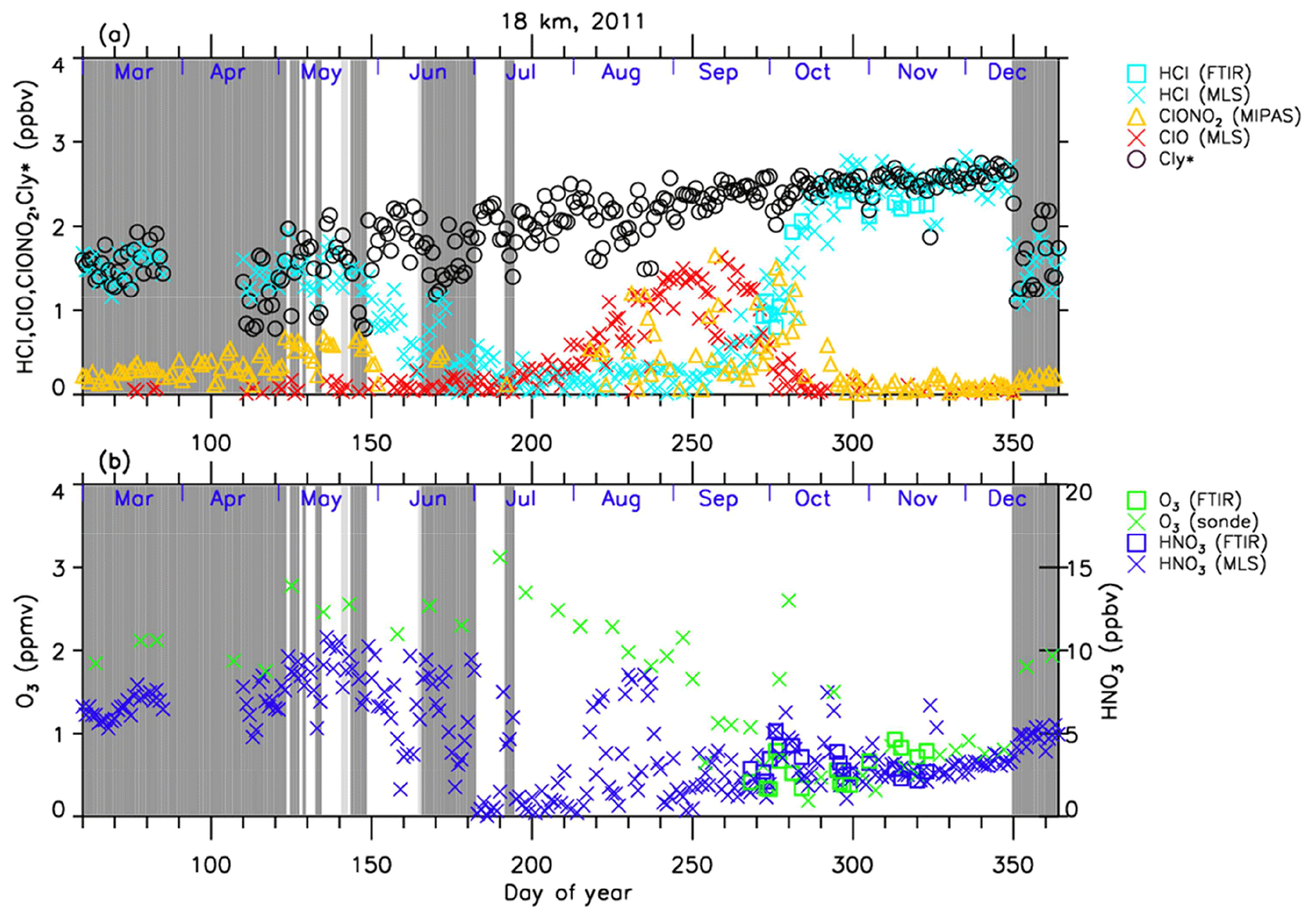
The altitude of 18 km was selected because it was one of the altitudes where nearly complete ozone loss occurred. The altitude of 22 km, where only about half of the ozone was depleted, was selected to show the difference in the behavior of chemical species from that at 18 km.

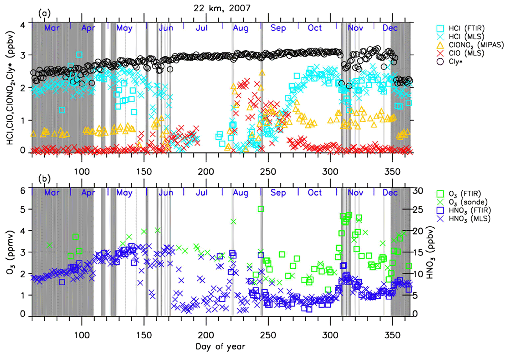
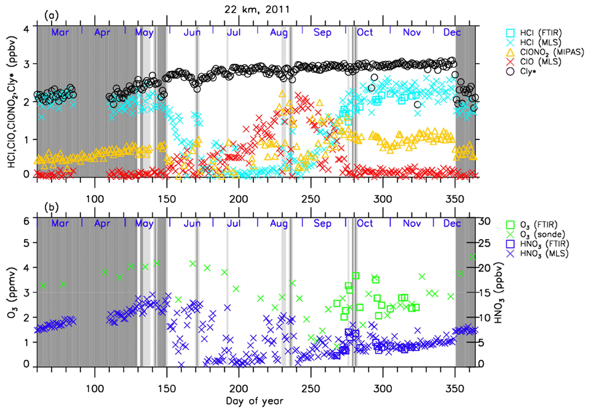
The general features of the chemical species observed inside the polar vortex at 18 and 22 km in 2007 and 2011 are summarized as follows: HCl and ClONO₂ decreased first, and then ClO started to increase in winter, while HCl increases and ClO decreases were synchronized in spring. HCl was almost zero from late June to early September, and the day-to-day variations were small over this period. HCl over Syowa Station indicates relatively larger values when it was located outside the polar vortex: for example, early August and the beginning of September at 22 km, 2007, in Fig. 6. HNO₃ showed large decreases from June to July and then gradually increased in summer. Day-to-day variations of HNO₃ from June to August were large. O₃ decreased from July to late September when ClO concentration was increased. ClO was enhanced in August and September, and the day-to-day variations were large over this period. ${\mathrm{Cl}}_y^{*}$ gradually increased in the polar vortex from late autumn to spring. The ${\mathrm{Cl}}_y^{*}$ value became larger compared with its mixing ratio outside of the polar vortex in spring.

The following characteristics are evident at 18 km (Figs. 4 and 5). O₃ gradually decreased from values of 2.5–3 ppmv before winter to values less than one-fifth, 0.3–0.5 ppmv, in October. The values of HCl from late June to early September were as small as 0–0.3 ppbv. The recovered values of HCl inside the vortex in spring (October–December) were larger than those before winter and those outside the polar vortex during the same period. ClONO₂ inside the vortex kept near zero even after ClO disappeared and did not recover to the level before winter until spring.

At 22 km (Figs. 6 and 7), O₃ gradually decreased from winter to spring, but the magnitude of the decrease was much smaller than that at 18 km. The values of HCl from late June to early September were 0–1 ppbv, which are larger than those at 18 km. The recovered values of HCl in spring were nearly the same as those before winter (around 2.2 ppbv). ClONO₂ recovered to larger values than those before winter after ClO disappeared.

As for the temporal increase in ClONO₂ in spring during the ClO decreasing phase, we can see a peak of 1.5 ppbv at 18 km in 2011 and at 22 km in both 2007 and 2011 around 27 September (day 270), but we see no temporal increase in ClONO₂ at 18 km in 2007.

Figure 7 shows that temporal ClO enhancement and decrease in O₃, ClONO₂, and HNO₃ occurred in early winter (30 May–19 June; day 150–170) at 22 km in 2011. This small ozone depletion event before winter may be due to an air mass movement from the polar night area to a sunlit area at lower latitudes.

4.2 Time series of ratios of chlorine species

In order to discuss the temporal variations of the chlorine partitioning, the ratios of observed HCl, ClONO₂, and ClO with respect to ${\mathrm{Cl}}_y^{*}$ were calculated. Hereafter, we will discuss the ratios of chlorine species only for the cases when Syowa Station was located inside the polar vortex.

Figures 8 and 9 show the time series of the ratios of each chlorine species with respect to ${\mathrm{Cl}}_y^{*}$ in 2007 (a) and in 2011 (b) at 18 and 22 km, respectively. In these plots, HCl data from Aura MLS were used. Note that light blue in these figures shows that either ClONO₂ or ClO data were missing on that day, while dark blue shows that all three data sets were available on that day. For both 2007 and 2011 at 18 km (Fig. 8), $\mathrm{HCl}/{\mathrm{Cl}}_y^{*}$ was 0.6–0.8 and ${\mathrm{ClONO}}_{\mathrm{2}}/{\mathrm{Cl}}_y^{*}$ was 0.2–0.3 before winter (10–20 May; day 130–140). The ratio of HCl to ${\mathrm{Cl}}_y^{*}$ was 3 times larger than that of ClONO₂ at that time. $\mathrm{ClO}/{\mathrm{Cl}}_y^{*}$ increased to ∼0.5 during the ClO-enhanced period (the period when ClO values were more than 80 % of its maximum value: 18 August–17 September; day 230–260). $\mathrm{HCl}/{\mathrm{Cl}}_y^{*}$ was 0–0.2 and ClONO₂/${\mathrm{Cl}}_y^{*}$ was 0-0.6 during this same period. ClONO₂ shows a negative correlation with ClO, while HCl remained low even when ClO was low during this period. This negative correlation is shown in Fig. 10. When ClO was enhanced, the O₃ amount gradually decreased and finally reached <0.5 ppmv (>80 % destruction) in October (7 October; day 280) (see Figs. 4 and 5). The ratios to ${\mathrm{Cl}}_y^{*}$ became 0.9–1.0 for HCl and 0–0.1 for ClONO₂ after the recovery in spring (after 17 October; day 290), indicating that almost all chlorine reservoir species became HCl via Reactions (R13) and/or (R14), due to the lack of O₃ and NO₂ during this period. The sum ratios $(\mathrm{HCl}+{\mathrm{ClONO}}_{\mathrm{2}}+\mathrm{ClO})/{\mathrm{Cl}}_y^{*}$ were around 0.5–0.8 at the time of the ClO-enhanced period. The remaining chlorine is thought to be either Cl₂O₂ or HOCl, which will be shown in model simulation result in Sect. 4.6. The sum ratio $(\mathrm{HCl}+{\mathrm{ClONO}}_{\mathrm{2}})/{\mathrm{Cl}}_y^{*}$ became close to 1 after the recovery period (after 7 October; day 280).

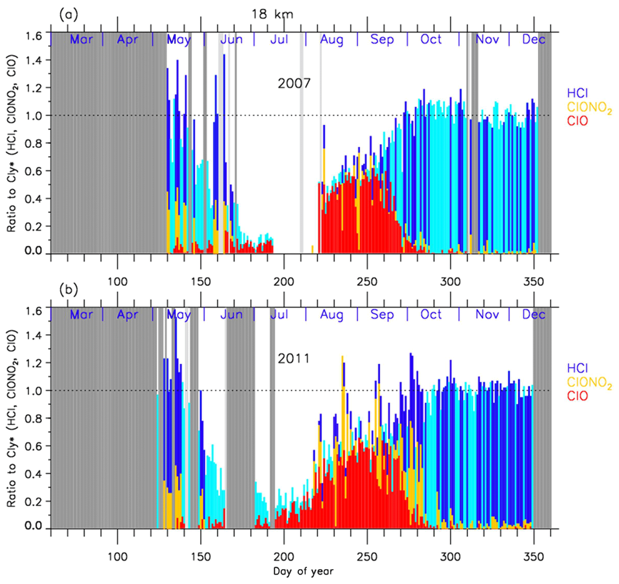
Figure 8 Time series of the ratios of HCl (dark blue or light blue), ClONO₂ (yellow), and ClO (red) to total chlorine (${\mathrm{Cl}}_y^{*}$) over Syowa Station at 18 km in (a) 2007 and in (b) 2011. Light blue shows that either ClONO₂ or ClO data were missing on that day, while dark blue shows that all three data sets were available on that day. Shaded areas are the same as Fig. 4.

Figure 9 Same as Fig. 8 but at 22 km.

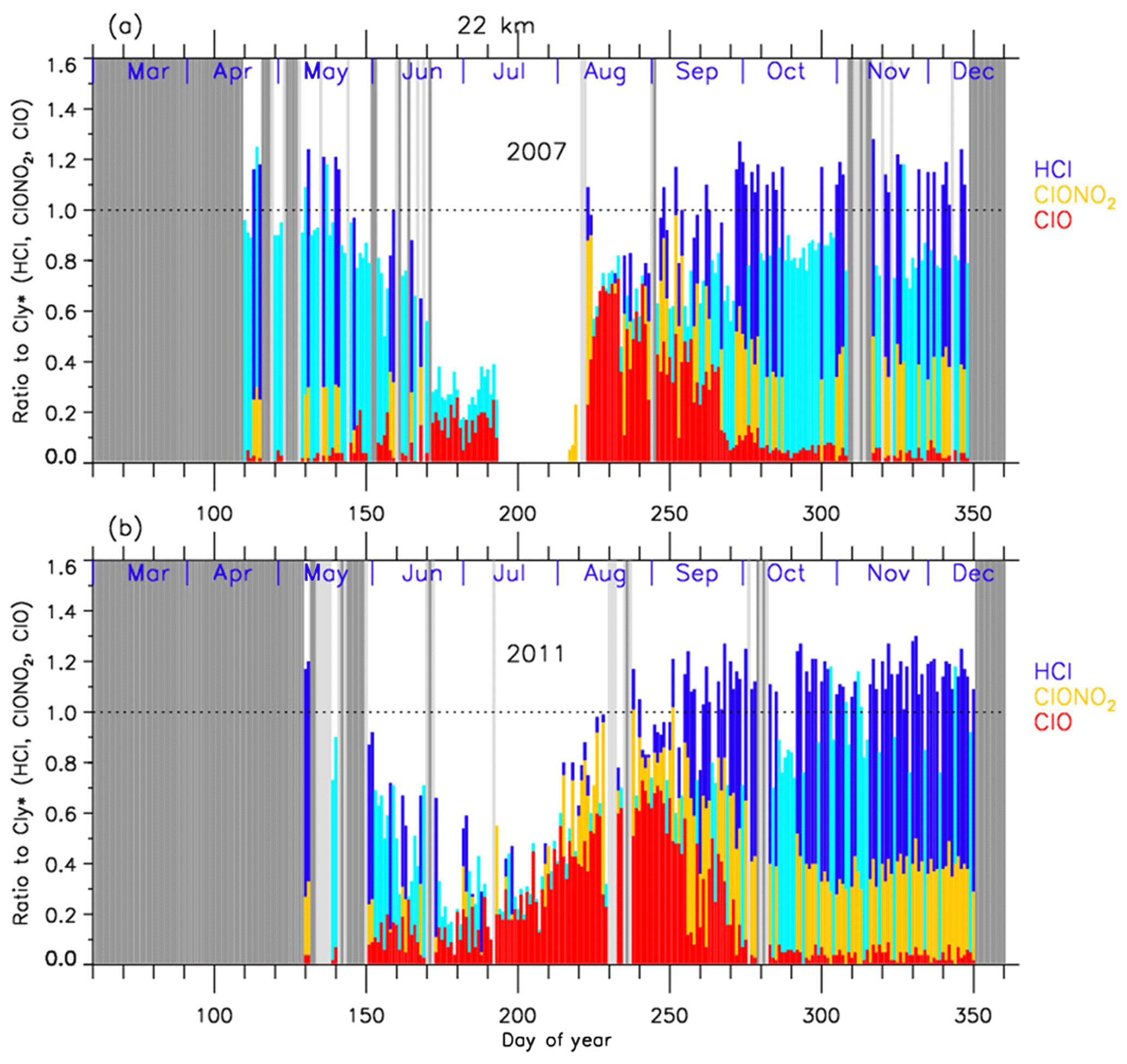
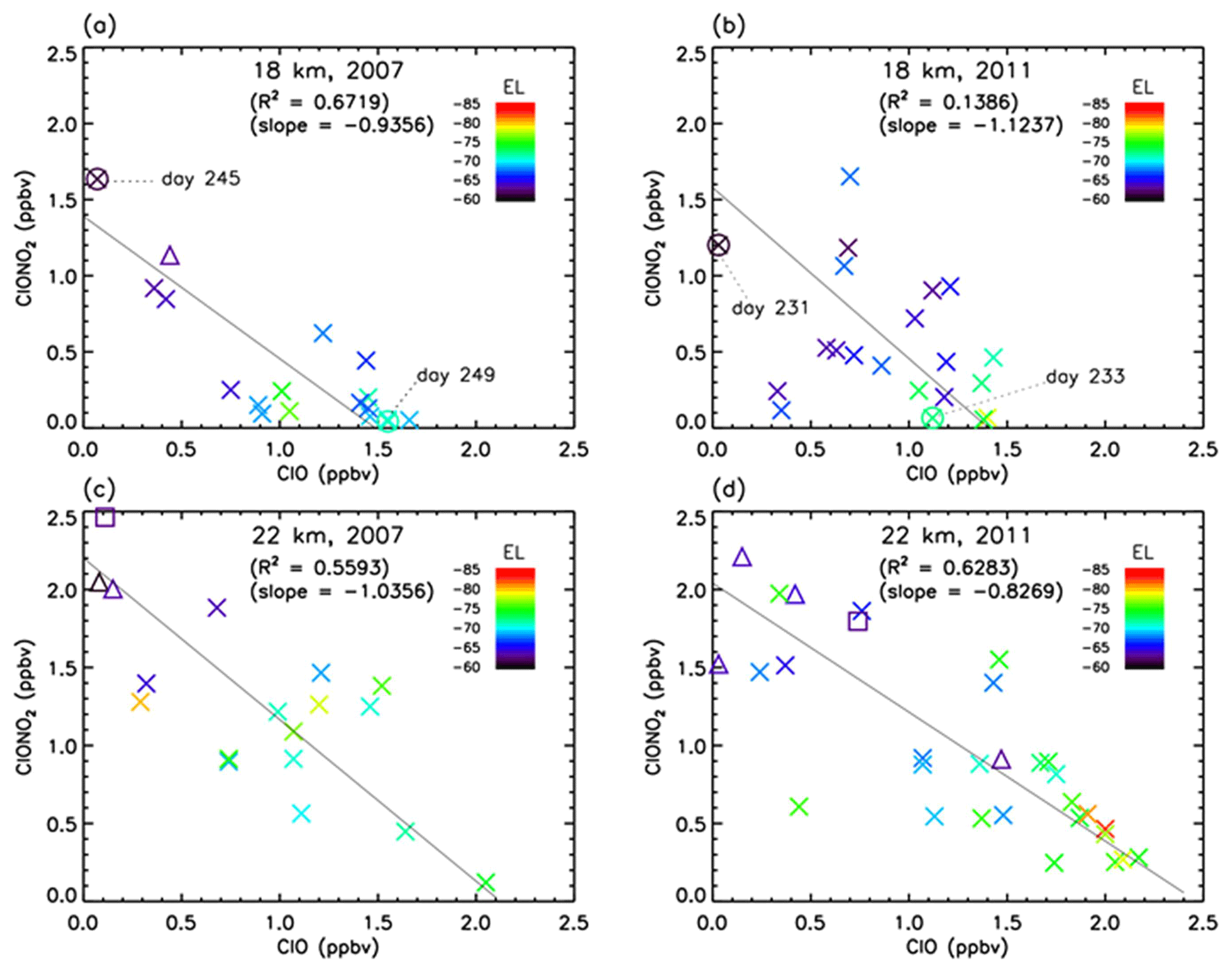
Figure 10 Scatter plot between ClO (Aura MLS) and ClONO₂ (Envisat MIPAS) mixing ratios between 8 August and 17 September (day 220–260) at 18 and 22 km in 2007 and 2011. Crosses, triangles, and squares represent the data when Syowa Station was located inside the polar vortex, in the boundary region of the polar vortex, and outside the polar vortex, respectively. Solid lines are regression lines obtained by reduced major axis (RMA) regression. Color represents the equivalent latitude over Syowa Station on that day. Circles with crosses represent the days which are shown in Figs. 13 and 14.

For both 2007 and 2011 at 22 km (Fig. 9), $\mathrm{HCl}/{\mathrm{Cl}}_y^{*}$ was 0.8–0.9 and ${\mathrm{ClONO}}_{\mathrm{2}}/{\mathrm{Cl}}_y^{*}$ was 0.2–0.3 before winter (20 April–20 May; day 110–140). The ratio of HCl to ${\mathrm{Cl}}_y^{*}$ was 3 to 4 times larger than that of ClONO₂. ClO/${\mathrm{Cl}}_y^{*}$ increased to 0.5–0.7 during the ClO-enhanced period (8–28 August – day 220–240 in 2007; 18 August–7 September – day 230–250 in 2011). $\mathrm{HCl}/{\mathrm{Cl}}_y^{*}$ was 0–0.2 and ${\mathrm{ClONO}}_{\mathrm{2}}/{\mathrm{Cl}}_y^{*}$ was 0–0.6 during this period. ClONO₂ shows a negative correlation with ClO, while HCl remained low even when ClO was low during this period as in the case at 18 km. The O₃ amount gradually decreased during the ClO-enhanced period but the concentration remained at more than 1.5 ppmv (less than half destruction) at this altitude (see Figs. 6 and 7). When the ClO enhancement ended, the increase in both ClONO₂ and HCl occurred simultaneously in early spring (17 September–7 October; day 260–280). Then the ratios to ${\mathrm{Cl}}_y^{*}$ became 0.6–0.7 for HCl and 0.3–0.4 for ClONO₂ in spring (after 7 October; day 280). This phenomenon shows that more chlorine deactivation via Reaction (R12) occurred towards ClONO₂ at 22 km rather than at 18 km. This is attributed to the existence of O₃ and NO₂ during this period at 22 km, which was different from the case at 18 km. The sum ratios $(\mathrm{HCl}+{\mathrm{ClONO}}_{\mathrm{2}}+\mathrm{ClO})/{\mathrm{Cl}}_y^{*}$ were around 0.7–1.2 at the time of the ClO-enhanced period. The remaining chlorine is thought to be either Cl₂O₂ or HOCl. The sum ratio $(\mathrm{HCl}+{\mathrm{ClONO}}_{\mathrm{2}}+\mathrm{ClO})/{\mathrm{Cl}}_y^{*}$ became around 1.2 after the recovery period (after 27 September; day 270). The reason why the observed sum ratio exceeds the calculated ${\mathrm{Cl}}_y^{*}$ value might be because the N₂O–Cl_y correlation from the one in Eq. (2) is not applicable at this altitude.

In 2011 at 18 km (Fig. 8), another temporal increase in ClONO₂ up to a ratio of 0.4 occurred in early spring (around 2–12 October; day 275–285) in accordance with the HCl increase, and then the ClONO₂ amount gradually decreased to nearly zero after late October (after 27 October; day 300). This temporal increase in ClONO₂ could be attributed to the temporal change of the location of Syowa Station with respect to the polar vortex. Although Syowa Station was judged to be inside the polar vortex during 14 July–16 December (day 195–350) by our analysis, the difference between the equivalent latitude over Syowa Station and that at the inner edge became less than 10^∘ on around 7 October (day 280), while it was typically between 15 and 20^∘ on other days. O₃ and HNO₃ showed higher values around 7 October (day 280) (see Fig. 5), indicating that Syowa Station was located close to the boundary region during this period (see Fig. B2 in Appendix B). Therefore, the temporal increase in ClONO₂ in 2011 at 18 km was attributed to spatial variation, not to chemical evolution.

4.3 Correlation between ClO and ClONO₂

Figure 10 shows the correlation between ClO and ClONO₂ during the ClO-enhanced period (8 August–17 September; day 220–260) at 18 km in 2007 (a) and 2011 (b) and at 22 km in 2007 (c) and 2011 (d). In this plot, the location of Syowa Station with respect to the polar vortex (inside, in the boundary region, and outside of the polar vortex) is indicated by different symbols. Note that MLS ClO and MIPAS ClONO₂ data were sampled on the same day at the nearest orbit to Syowa Station for both satellites. The maximum differences between these two satellites' observational times and locations are 9.0 h in time and 587 km in distance. Mean differences are 6.8 h in time and 270 km in distance, respectively. Solid lines show regression lines obtained by reduced major axis (RMA) regression. Negative correlations of slope of about −1.0 between ClO and ClONO₂ are seen in all figures.

The negative correlation between ClO and ClONO₂ at Syowa Station is explained by the difference in the concentration of ClO, NO₂, ClONO₂, and HNO₃ inside, outside, and at the boundary region of the polar vortex around the station. Outside of the polar vortex, the ClO concentration is lower and NO₂ concentration is higher than those inside the polar vortex. Inside the polar vortex, HNO₃ is taken up by PSCs and removed by the sedimentation of PSCs from the lower stratosphere (denitrification process). The NO_x concentration is low because HNO₃ is a reservoir of NO_x through the reactions

$$\begin{array}{}\text{(R17)}& {\displaystyle }{\mathrm{NO}}_{\mathrm{2}}+\mathrm{OH}+M\to {\mathrm{HNO}}_{\mathrm{3}}+M,\text{(R18)}& {\displaystyle }{\mathrm{HNO}}_{\mathrm{3}}+h\mathit{\nu }\to {\mathrm{NO}}_{\mathrm{2}}+\mathrm{OH},\end{array}$$

and

$$\begin{array}{}\text{(R19)}& {\mathrm{HNO}}_{\mathrm{3}}+\mathrm{OH}\to {\mathrm{NO}}_{\mathrm{3}}+{\mathrm{H}}_{\mathrm{2}}\mathrm{O}.\end{array}$$

The NO₂ concentration is low and ClONO₂ concentration is also low due to the consumption of ClONO₂ by the heterogeneous Reaction (R2) inside the polar vortex. In spring, the ClO amount increases due to the activation of chlorine species by Reactions (R1)–(R8) inside the polar vortex. At the boundary region, ClO and NO₂ concentrations indicate the value between the inside and outside of the polar vortex; that is, the ClO concentration is much higher than that outside of the polar vortex and NO₂ concentration is much higher than that inside of the polar vortex. Thus, the ClONO₂ concentration there is elevated in August–September due to Reaction (R12). This causes the negative correlation between ClO and ClONO₂ due to the relative distance between Syowa Station and the edge of the polar vortex. When Syowa Station was located deep inside the polar vortex, there was more ClO and less ClONO₂. On the contrary, when Syowa Station was located near the vortex edge, there was less ClO and more ClONO₂. The equivalent latitude (EL) over Syowa Station was calculated as described in Appendix B for each correlation point. The EL at each correlation point is now shown by the color code in Fig. 10. It generally shows the tendency that warm-colored higher equivalent latitude points are located more towards the bottom right-hand side. This is further confirmed by three-dimensional model simulation as shown later.

4.4 Comparison with model results

Figures 11 and 12 show comparisons of daily time series of simulated mixing ratios of ClO, HCl, ClONO₂, Cl_y, and O₃ by the MIROC3.2 chemistry–climate model (Akiyoshi et al., 2016) with FTIR, Aura MLS, and Envisat MIPAS measurements at 18 and 22 km. For a description of the MIROC3.2 CCM, please see Appendix A. In these figures, Cl_y for Aura MLS in the panels (d) and (i) actually represents the ${\mathrm{Cl}}_y^{*}$ value calculated by Eq. (2) using the N₂O value measured by Aura MLS. Cl_y from the MIROC3.2 CCM is the sum of total reactive chlorines; i.e., ${\mathrm{Cl}}_y=\mathrm{Cl}+\mathrm{2}\cdot {\mathrm{Cl}}_{\mathrm{2}}+\mathrm{ClO}+\mathrm{2}\cdot {\mathrm{Cl}}_{\mathrm{2}}{\mathrm{O}}_{\mathrm{2}}+\mathrm{OClO}+\mathrm{HCl}+\mathrm{HOCl}+{\mathrm{ClONO}}_{\mathrm{2}}+{\mathrm{ClNO}}_{\mathrm{2}}+\mathrm{BrCl}$. Note that we plotted modeled values at 12:00 UTC (∼ 15:00 local time of Syowa Station) calculated by the MIROC3.2 CCM in order to compare the daytime measurements of FTIR and satellites. In Fig. 11b, d, g, and i, modeled HCl and Cl_y are systematically smaller by 20 %–40 % compared with FTIR or MLS measurements. The cause of this discrepancy may be partly due to either smaller downward advection and/or faster horizontal mixing of an air mass across the subtropical barrier in MIROC3.2 CCM (Akiyoshi et al., 2016). Nevertheless, evolutions of measured ClO and ClONO₂ for the period are well simulated by the MIROC3.2 CCM. Modeled O₃ were in very good agreement with FTIR and/or MLS measurements throughout the year in both altitudes for both years. Hereafter, the result of MIROC3.2 CCM at 50 hPa (∼18 km) is discussed.

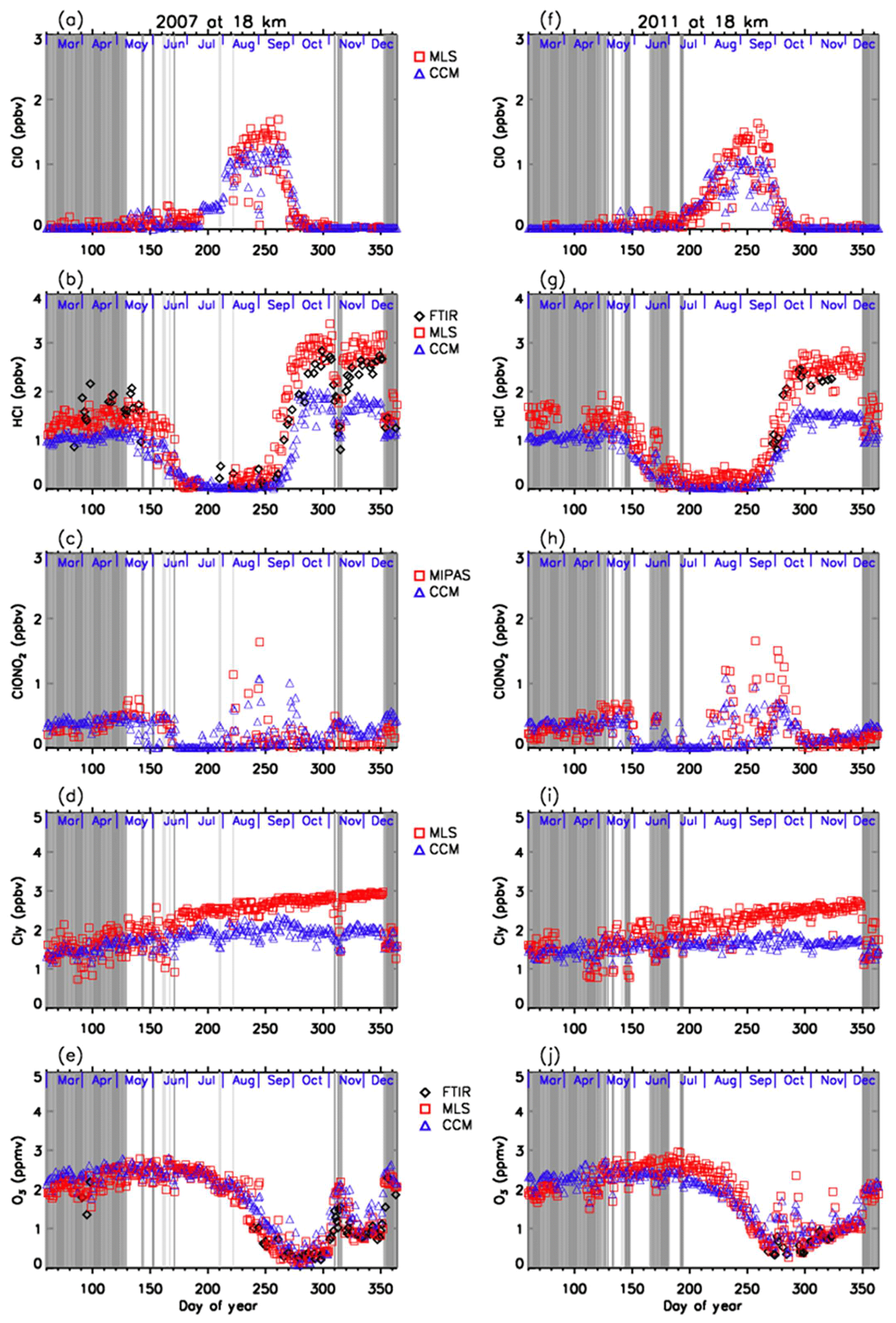
Figure 11 Daily time series of measured and modeled minor species over Syowa Station at 18 km. Black diamonds are data by FTIR, red squares are by Aura MLS and Envisat MIPAS, blue triangles are data by MIROC3.2 CCM. Panel (a) is for ClO, (b) is for HCl, (c) is for ClONO₂, (d) is for Cl_y, and (e) is for O₃ in 2007. (f) is for ClO, (g) is for HCl, (h) is for ClONO₂, (i) is for Cl_y, and (j) is for O₃ in 2011.

Figure 12 Same as Fig. 11 but for 22 km.

4.5 Polar distribution of minor species

Figure 13 shows distributions of temperature from the model nudged toward the ERA-Interim data and simulated mixing ratios of O₃, NO₂, HNO₃, ClO, HCl, and ClONO₂ by the MIROC3.2 CCM at 50 hPa for 24 June (day 175), 2 September (day 245), 6 September (day 249), and 6 October (day 279) in 2007. Polar vortex edges defined by the method described in Appendix B were plotted with white outlines. The location of Syowa Station is shown by a white star in each panel. On 24 June (day 175), stratospheric temperatures over Antarctica were already low enough for the onset of heterogeneous chemistry. Consequently, NO₂ was converted into HNO₃ via Reaction (R17), and HNO₃ in the polar vortex was condensed onto PSCs. Note that the depleted area of NO₂ was greater than that of HNO₃. This is due to the occurrence of Reaction (R12) that converts ClO and NO₂ into ClONO₂ at the edge of the polar vortex, which is shown by the enhanced ClONO₂ area at the vortex edge in Fig. 13. Also, HCl and ClONO₂ are depleted in the polar vortex due to the heterogeneous Reactions (R1), (R2), (R3), and (R4) on the surface of PSCs and aerosols. Some HCl remains near the core of the polar vortex, because the initial amount of the counterpart of the heterogeneous Reaction (R1) (ClONO₂) was less than that of HCl, as was also shown by CLaMS, SD-WACCM, and TOMCAT/SLIMCAT model simulations by Grooß et al. (2018). The O₃ amount was only slightly depleted within the polar vortex on this day.

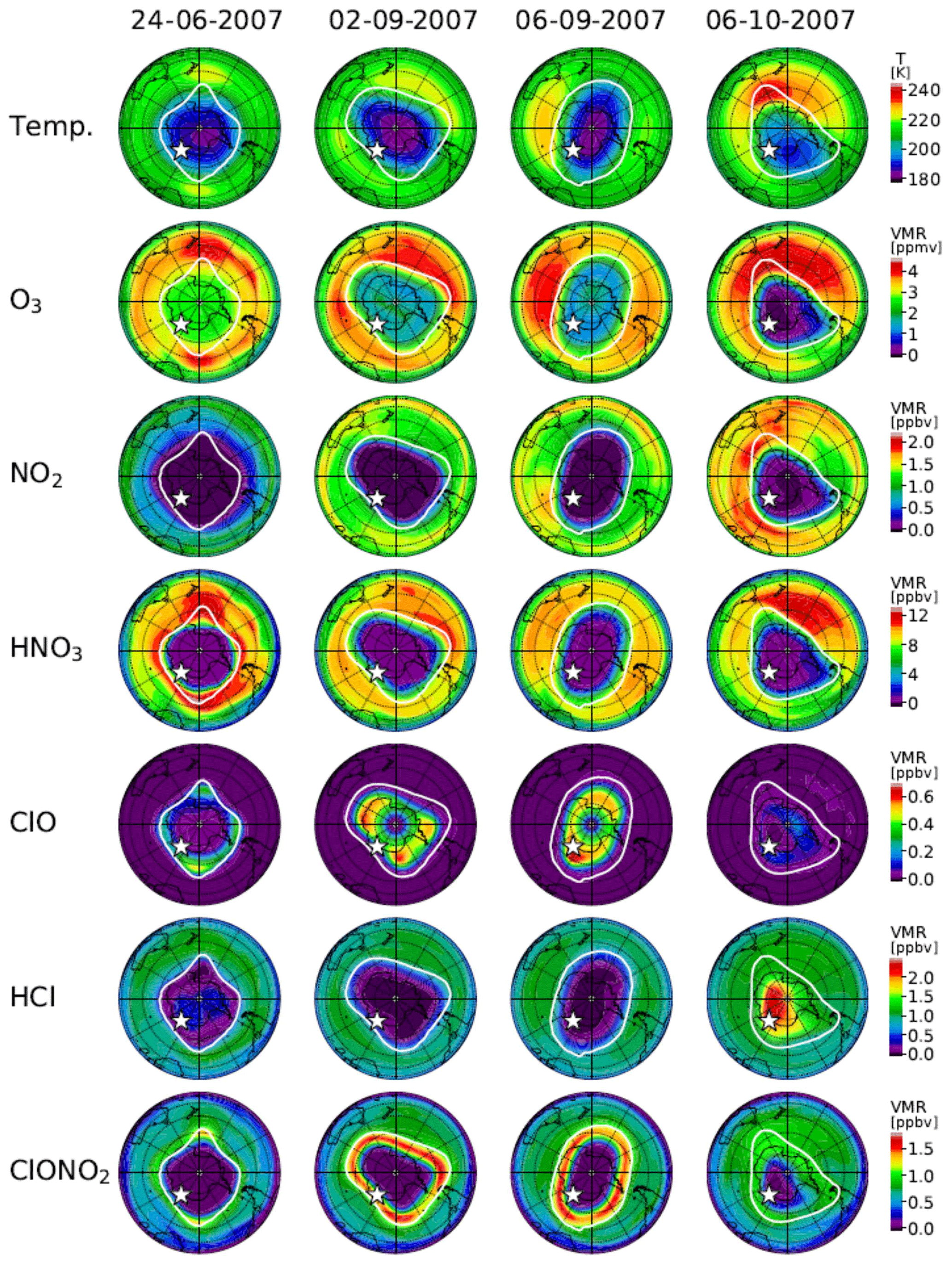
Figure 13 Polar southern hemispheric plots for ERA-Interim temperature and simulated mixing ratios of O₃, NO₂, HNO₃, ClO, HCl, and ClONO₂ by a MIROC3.2 chemistry–climate model (CCM) at 50 hPa for 24 June (day 175), 2 September (day 245), 6 September (day 249), and 6 October (day 279), 2007. The polar vortex (outer) edge defined as the method described in Appendix B at 450 K was plotted by a white outline in each panel. The location of Syowa Station was shown by a white star in each panel.

On 2 September (day 245), amounts of NO₂, HNO₃, HCl, and ClONO₂ all show very depleted values in the polar vortex. The amount of ClO shows some enhanced values inside the polar vortex. The development of ozone depletion was seen in the polar vortex. Note that ClONO₂ shows enhanced values around the boundary region of the polar vortex. This might be due to Reaction (R12) at this location. On this day (day 245), Syowa Station was located inside the polar vortex close to the vortex edge, where ClO was smaller and ClONO₂ was greater than the values deep inside the polar vortex as observed and indicated by the upper-left circle with a cross in Fig. 10a.

On 6 September (day 249), most features were the same as on 2 September, but the shape of the polar vortex was different. Consequently, Syowa Station was located deep inside the polar vortex, where ClO was greater and ClONO₂ was smaller than the values around the boundary region of the polar vortex as observed and indicated by the lower-right circle with a cross in Fig. 10a. Hence, the negative correlation between ClO and ClONO₂ seen in Fig. 10 was due to variation of the relative distance between Syowa Station and the edge of the polar vortex.

As for HCl, it remained near zero not only on this day (6 September) but also on 2 September when Syowa Station was located inside the polar vortex close to the vortex edge. Therefore, observed day-to-day variations of HCl were small and did not show any correlation with ClO (see Figs. 4–7). A possible explanation to keep a near zero HCl value close to the vortex edge is due to so-called “HCl null cycles”, which were started with Reaction (R13), proposed by Müller et al. (2018). This cycle is discussed later.

On 6 October (day 279), ClO enhancement has almost disappeared. Inside the polar vortex, O₃, NO₂, HNO₃, and ClONO₂ showed very low values. Ozone was almost fully destroyed at this altitude in the polar vortex. However, the amount of HCl increased deep inside the polar vortex. This might be due to the recovery of HCl by Reactions (R13) and/or (R14) deep inside the polar vortex, where there was no O₃ or NO₂ left and Reactions (R13) and/or (R14) were favored compared with Reaction (R12). Syowa Station was located deep inside the polar vortex, and the simulated and observed amounts of HCl were both more than 10 times greater than those of ClONO₂ on this day (see Fig. 4).

Figure 14 shows distributions of temperature from the model nudged toward the ERA-Interim data and simulated mixing ratios of O₃, NO₂, HNO₃, ClO, HCl, and ClONO₂ by the MIROC3.2 CCM at 50 hPa for 5 July (day 186), 19 August (day 231), 21 August (day 233), and 9 October (day 282) in 2011. The polar vortex edges and location of Syowa Station were also plotted. On 5 July (day 186), the situation was similar to that of 24 June (day 175) in 2007. Note that the inner edge of the polar vortex was defined on this day. Syowa Station was located deeper inside the polar vortex on 5 July in 2011 than on 24 June in 2007, and the remaining HCl was observed by MLS (see Fig. 5).

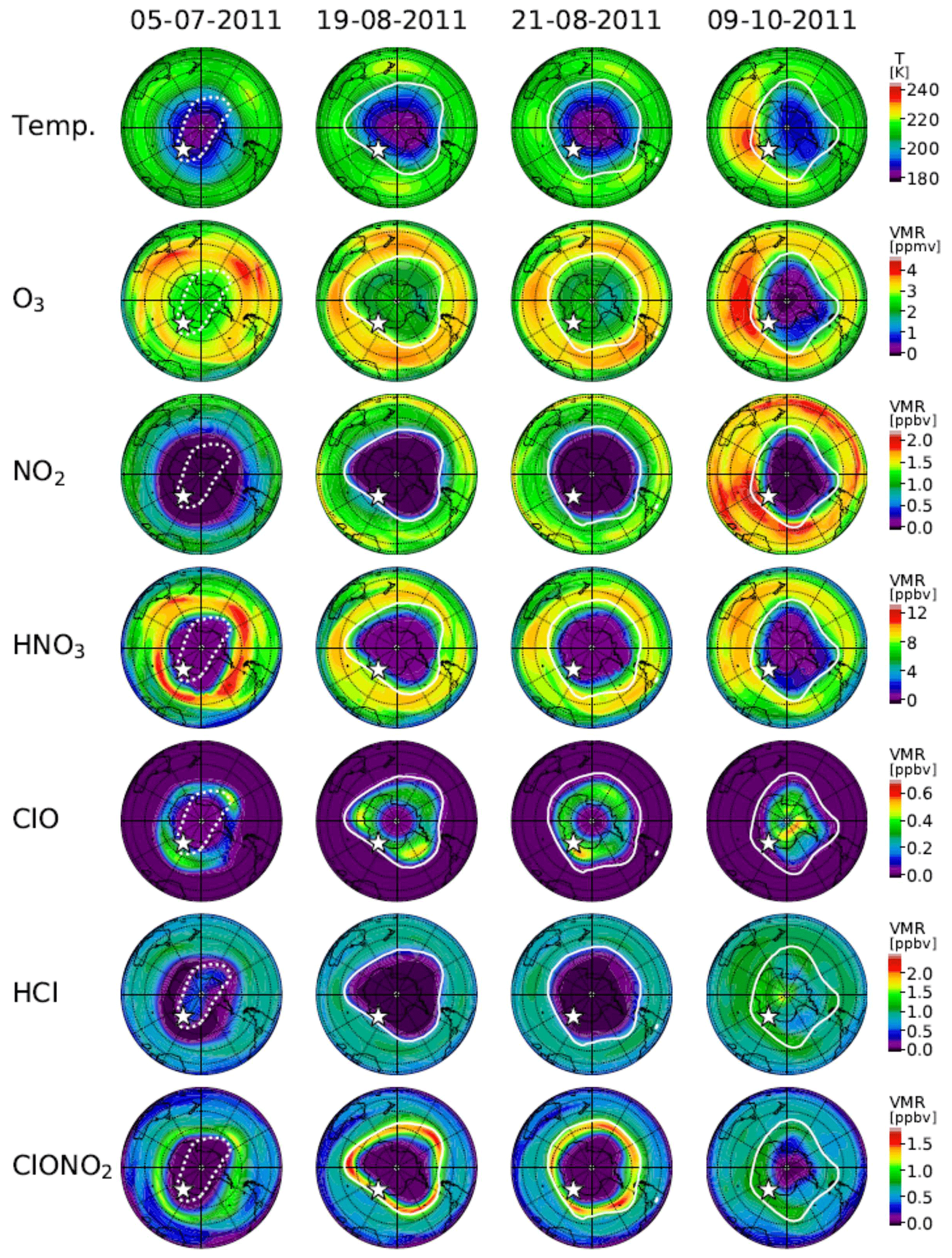
Figure 14 Same as Fig. 13 but for 5 July (day 186), 19 August (day 231), 21 August (day 233), and 9 October (day 282), 2011. The polar vortex edge on 5 July plotted by a dotted while outline indicates that the inner vortex edge was defined on this day.

On 19 August (day 231) and 21 August (day 233), the situations were similar to those of 2 September (day 245) and 6 September (day 249) in 2007, respectively. ClO and ClONO₂ correlations on these days are also indicated by circles with crosses in Fig. 10b.

On 9 October (day 282), the situation was similar to that of 6 October (day 279) in 2007, but Syowa Station was located inside the polar vortex closer to the inner vortex edge than in 2007. The recovery of ClONO₂ by Reaction (R12) was simulated and observed at Syowa Station in addition to the recovery of HCl by Reaction (R13) (see Fig. 8b), because there were some remaining O₃ and NO₂ air masses near the inner vortex edge (see Fig. 5). This shows the phenomena described on the last paragraph in Sect. 4.2.

4.6 Time evolution of chlorine species from CCM and discussion

Three-hourly time series of zonal-mean active chlorine species, Cl₂O₂ (b), Cl₂ (c), ClO (d), and their sum ($\mathrm{ClO}+\mathrm{2}\cdot {\mathrm{Cl}}_{\mathrm{2}}{\mathrm{O}}_{\mathrm{2}}+\mathrm{2}\cdot {\mathrm{Cl}}_{\mathrm{2}}$) (a), HOCl (e), and chlorine reservoir species HCl (f) and ClONO₂ (g) modeled by MIROC3.2 CCM at 68.4, 71.2, 76.7, and 87.9^∘ S in 2007 are plotted in Fig. 15. The dates on which the distribution of each species is shown in Fig. 13 are indicated by vertical dotted lines. In Fig. 15, it is shown that HCl and ClONO₂ rapidly decreased on around 10 May (day 130) at 87.9^∘ S due to the heterogeneous Reaction (R1), when PSCs started to form in the Antarctic polar vortex (Fig. 15f and g). Consequently, Cl₂ was formed (Fig. 15c). Similar chlorine activation was seen at 76.7^∘ S about 5–10 d later than at 87.9^∘ S. The decrease in HCl stopped when the counterpart of the heterogeneous Reaction (R1) (ClONO₂) was missing on around 20 May (day 140). The continuous loss of HCl occurred from June to July (day 160–200). The possible cause of this loss will be discussed later. Gradual conversion from Cl₂ into Cl₂O₂ (ClO dimer) was seen at all latitudes on around 30 May–9 June (day 150–160) (Fig. 15b and c) through Reactions (R5), (R8), and (R9). At 87.9^∘ S, conversion from Cl₂ to Cl₂O₂ was slow, due to the lack of sunlight, which is needed for Reaction (R5). The increase in ClO occurred much later in winter (9 July; day 190 or later), because sunlight is needed to form ClO by Reactions (R5) and (R8) in the polar vortex (Fig. 15d). Nevertheless, there were some enhancements of ClO in early winter, on 24 June (day 175), simulated at the edge of the polar vortex (Fig. 13) where there was some sunlight available due to the distortion of the shape of the polar vortex. The increase in ClO occurred from a lower latitude (68.4^∘ S) on around 14 July (day 195) towards a higher latitude (87.9^∘ S) on around 12 September (day 255) (Fig. 15d). Diurnal variation of ClO was also seen at latitudes between 68.4 and 76.7^∘ S. When the stratospheric temperature increased above NAT saturation temperature on around 27 September (day 270) (Fig. 3b), chlorine activation ended, and ClO was mainly converted into HCl at all latitudes inside the polar vortex (Fig. 15d and f). This is because Reactions (R13) and/or (R14) occur more frequently than Reaction (R12) inside the polar vortex due to the depleted O₃ amount there, as was described in Sect. 1 (Douglass et al., 1995). The increase in HOCl due to the heterogeneous Reaction (R2) on the surface of PSCs occurred gradually from June at lower latitudes (68.4 and 71.2^∘ S) (Fig. 15e). It also occurred at 76.7^∘ S from July and at 87.9^∘ S from August. The cause of the HOCl increase at 87.9^∘ S from August is not clear at the moment. In Fig. 15, the species which decreased at 87.9^∘ S from August was Cl₂ (Fig. 15c). If sunlight was available, Cl₂ was converted into HOCl through Reactions (R5) and (R8) as well as the following reaction:

$$\begin{array}{}\text{(R20)}& \mathrm{ClO}+{\mathrm{HO}}_{\mathrm{2}}\to \mathrm{HOCl}+{\mathrm{O}}_{\mathrm{2}}.\end{array}$$

Here, HO₂ was needed to yield HOCl. One possibility to yield HO₂ in August is either one of the HCl null cycles C₁ or C₂ (see Appendix C) or one of the HCl destruction cycles C₃ or C₄ (see Appendix C), which was described in Müller et al. (2018). If the air mass at 87.9^∘ S was located equatorward due to the obliqueness of the polar vortex a few days earlier, then sunlight may have been available and such reactions could yield HOCl at 87.9^∘ S.

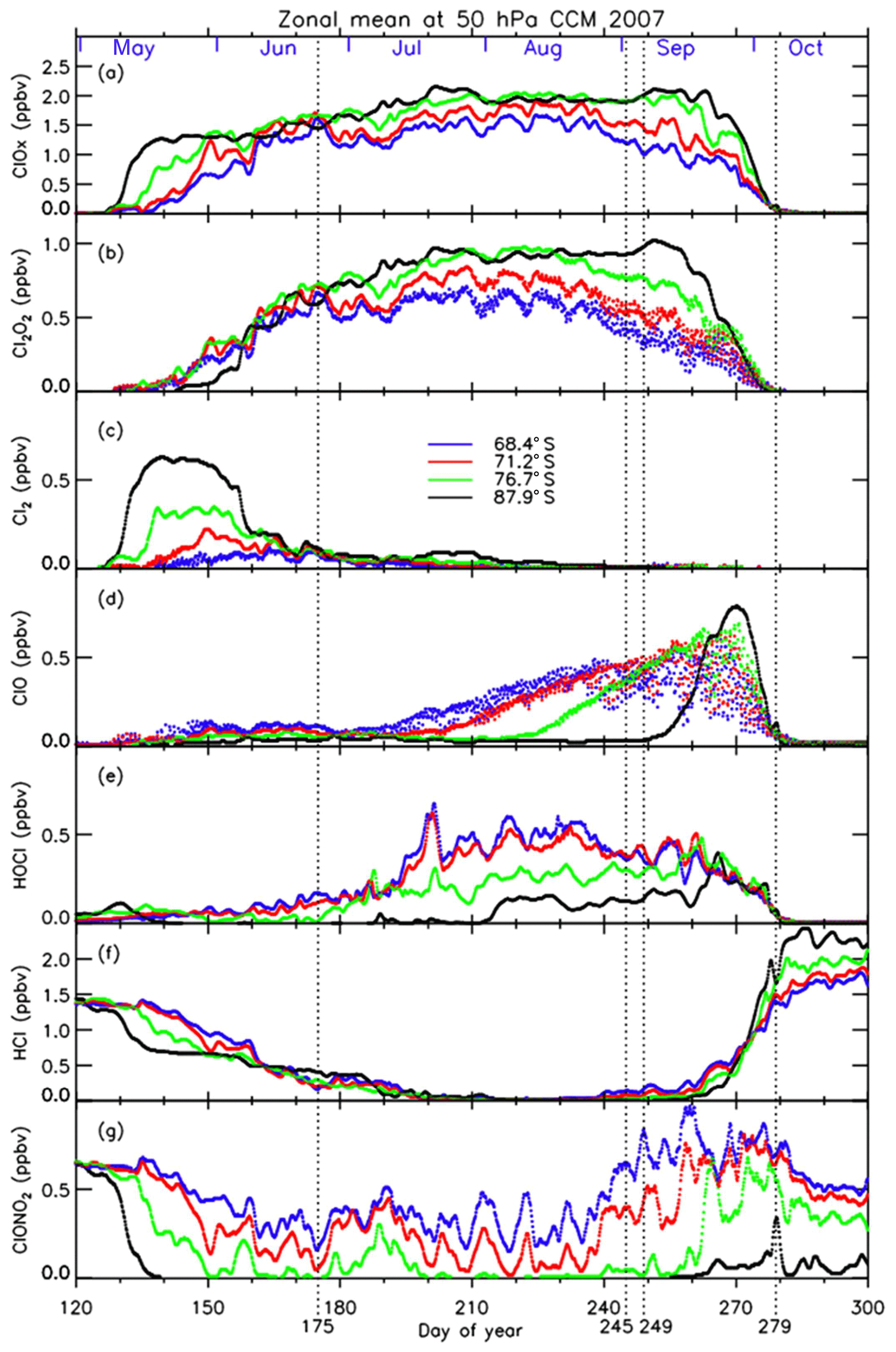
Figure 15 Three-hourly zonal-mean time series of MIROC3.2 CCM outputs for (a) $\mathrm{ClO}+\mathrm{2}\cdot {\mathrm{Cl}}_{\mathrm{2}}{\mathrm{O}}_{\mathrm{2}}+\mathrm{2}\cdot {\mathrm{Cl}}_{\mathrm{2}}$, (b) Cl₂O₂, (c) Cl₂, (d) ClO, (e) HOCl, (f) HCl, and (g) ClONO₂ during day number 120–300 at 50 hPa in 2007.

The continuous loss of HCl was seen at 87.9^∘ S between 9 June (day 160) and 19 July (day 200) even after the disappearance of the counterpart of the heterogeneous Reaction (R1) (Fig. 15f). The cause of this continuous loss was unknown until recently, where a hypothesis was proposed that includes the effect of decomposition of particulate HNO₃ by some processes like ionization of air molecules caused by galactic cosmic rays during the winter polar vortex or photolysis of dissolved HNO₃ in PSC particles (Grooß et al., 2018). However, they concluded that these processes could not explain the HCl discrepancy between their models and observations. We consider that the continuous loss of HCl was caused by the mixing of ClONO₂-containing air with the air at the core of the polar vortex, due to the excursions of air parcels in and out of sunlight during the winter caused by the distortion of the polar vortex, which photochemically resupply ClONO₂ and HOCl. Our result was indicated by some sporadic increase in ClONO₂ on around 7 June (day 158), 28 June (day 179), and 8 July (day 189) at 76.7^∘ S as shown in Fig. 15g. We confirmed that the shapes of the polar vortex were rather distorted on these days. Subsequently, HCl losses were observed at 76.7 and 87.9^∘ S during these episodes in Fig. 15f. Thus, the continuous loss of HCl at the most polar latitude (87.9^∘ S) could be due to the gradual mixing of air within the polar vortex during the winter period, when the polar vortex was still strong.

The ClONO₂ distribution on 24 June 2007 in Fig. 13 shows a peak at around the polar vortex outer edge (equivalent latitude of ∼62^∘ S) where there was no HCl. We confirmed that such a peak continued to exist from the middle of June to the end of July, when sunlight was not available at a geographical latitude higher than 70^∘ S due to polar night. However, a substantial amount of ClONO₂ exists between an equivalent latitude of 62^∘ S (polar vortex outer edge) and 70^∘ S, mainly due to the distortion of the polar vortex and availability of O₃. At 62^∘ S equivalent latitude, the amount of ClONO₂ has a peak around these days, while HCl amounts were low. At around 65–70^∘ S, HCl was almost fully depleted. Therefore, if the air mass which contains some ClONO₂ traveled poleward due to mixing, it could react with HCl by Reaction (R1) and continuously destroy HCl in the core of the polar vortex during the polar night in June and July. Another explanation for the loss of HCl is the heterogeneous Reaction (R4) on the surface of PSCs with HOCl. Spiky increases in HOCl at 76.7 and 87.9^∘ S and a simultaneous decrease in HCl occurred on around 7 July (day 188) and 20 July (day 201) in Fig. 15e and f. The continuous loss of HCl at the core of the polar vortex in August and September was recently proposed by Müller et al. (2018), who proposed that HCl destruction cycles C₃ and C₄ (see Appendix C) are responsible for the decline of HCl in the vortex core. These chemical cycles also require sunlight to occur, which may not be available in June and July at the vortex core. Therefore, the distortion of the polar vortex is also important for that reaction to occur as well. We consider that the reactions of HCl with both ClONO₂ and HOCl contribute the continuous loss of HCl during winter in the vortex core.

Recently, Solomon et al. (2015) discussed the race between chlorine activation and deactivation to maintain enhanced levels of active chlorine during the time period (September and early October) when rapid ozone loss occurs. Müller et al. (2018) proposed so-called HCl null cycles to maintain enhanced chlorine levels. They proposed a mechanism in which the formation of HCl (Reaction R13) is followed by the immediate reactivation of HCl by null cycles C₁ and C₂ (see Appendix C) (Müller et al., 2018). Our MIROC3.2 CCM model results support the mechanism by high ClO and HOCl levels in September as shown in Fig. 15d and e.

5 Conclusions

Lower stratospheric vertical profiles of O₃, HNO₃, and HCl were retrieved using SFIT2 from solar spectra taken with a ground-based FTIR installed at Syowa Station, Antarctica, from March to December 2007 and September to November 2011. This was the first continuous measurement of chlorine species throughout the ozone hole period from the ground in Antarctica. Retrieved profiles were validated with Aura MLS and ozonesonde data. The absolute differences between FTIR and Aura MLS or ozonesonde measurements were within measurement error bars at the altitudes of interest.

To study the temporal variation of chlorine partitioning and ozone destruction from fall to spring in the Antarctic polar vortex, we analyzed temporal variations of measured minor species using FTIR over Syowa Station combined with satellite measurements of ClO, HCl, ClONO₂ and HNO₃. When the stratospheric temperature over Syowa Station fell ∼4 K below NAT saturation temperature, PSCs started to form and the heterogeneous reaction between HCl and ClONO₂ occurred, and eventually, in early winter, both HCl and ClONO₂ were almost completely depleted at both 18 and 22 km. When the sun came back to the Antarctic in spring, enhancement of ClO and gradual O₃ destruction were observed. During the ClO-enhanced period, a negative correlation between ClO and ClONO₂ was observed in the time series of the data at Syowa Station. This negative correlation is associated with the relative distance between Syowa Station and the edge of the polar vortex.

To investigate the behavior of whole chlorine and related species inside the polar vortex and the boundary region in more detail, results of the MIROC3.2 CCM simulation were analyzed. The direct comparison between CCM results and observations shows good day-to-day agreement in general, although some species show systematic differences especially at 18 km. The modeled O₃ is in good agreement with FTIR and satellite observations. Rapid conversion of chlorine reservoir species (HCl and ClONO₂) into Cl₂, gradual conversion of Cl₂ into Cl₂O₂, increase in HOCl in the winter period, increase in ClO when sunlight became available, and conversion of ClO into HCl were successfully reproduced by the CCM. The HCl decrease in the winter polar vortex core continued to occur due to both transport of ClONO₂ from the polar vortex boundary region to higher latitudes, providing a flux of ClONO₂ from more sunlit latitudes into the polar vortex, and the heterogeneous reaction of HCl with HOCl. The temporal variation of chlorine species over Syowa Station was affected by both heterogeneous chemistries related to PSC occurrence inside the polar vortex and transport of a NO_x-rich air mass from the polar vortex boundary region, which can produce additional ClONO₂ via Reaction (R12).

The deactivation pathways from active ClO into reservoir species (HCl and/or ClONO₂) were confirmed to be very dependent on the availability of ambient O₃. At 18 km, where most ozone was depleted, most ClO was converted to HCl. At 22 km, when some O₃ was available, an additional increase in ClONO₂ than the prewinter value occurred, similar to the Arctic, through Reactions (R15) and (R12) (Douglass et al., 1995; Grooß et al., 1997).

Appendix A: MIROC3.2 nudged chemistry–climate model

The chemistry–climate model used in this study was the MIROC3.2 CCM, which was developed on the basis of version 3.2 of the Model for Interdisciplinary Research on Climate (MIROC3.2) general circulation model (GCM). The MIROC3.2 CCM introduces the stratospheric chemistry module of the old version of the CCM that was used for simulations proposed by the chemistry–climate model validation (CCMVal) and the second round of CCMVal (CCMVal2) (WMO, 2007, 2011; SPARC CCMVal, 2010; Akiyoshi et al., 2009, 2010). The MIROC3.2 CCM is a spectral model with a T42 horizontal resolution (2.8^∘ × 2.8^∘) and 34 vertical atmospheric layers above the surface. The top layer is located at approximately 80 km (0.01 hPa). Hybrid sigma–pressure coordinates are used for the vertical coordinate. The horizontal wind velocity and temperature in the CCM were nudged toward the ERA-Interim data (Dee et al., 2011) to simulate global distributions of ozone and other chemical constituents on a daily basis. The transport is calculated by a semi-Lagrangian scheme (Lin and Rood, 1996). The chemical constituents included in this model are O_x, HO_x, NO_x, ClO_x, BrO_x, hydrocarbons for methane oxidation, heterogeneous reactions on the surface for sulfuric acid aerosols, supercooled ternary solutions, nitric acid trihydrate, and ice particles.

Table A1 FTIR observation dates at Syowa Station in 2007 and 2011.

The CCM contains 13 heterogeneous reactions on multiple aerosol types (Akiyoshi, 2007) as well as gas-phase chemical reactions and photolysis reactions. The surface of the particles for the heterogeneous reactions is calculated from the volume of condensation, assuming number density of the particles and the size distributions. Additionally, sedimentation of the particles is considered. The reaction-rate and absorption coefficients are based on JPL-2010 (Sander et al., 2011). The family method is used to calculate gas-phase chemical reactions. The time integrations for the families and heterogeneous reactions are performed explicitly. The time step for the chemistry scheme is 6 min. A scheme of spherical geometry for radiation transfer was developed (Kurokawa et al., 2005) and used for radiation transfer calculation in the CCM. The photolysis rates of chemical constituents are calculated online, using the radiation flux in the CCM with 32 spectral bins. All the 42 photolysis reactions, 140 gas-phase reactions, and 13 heterogeneous reactions are summarized in Table A2. See Akiyoshi et al. (2016) and the Supplement of Morgenstern et al. (2017) for more details.

Table A2 Chemical reactions in the MIROC3.2 chemistry–climate model.

Total: 42 photolysis reactions, 140 gas-phase reactions, and 13 heterogeneous reactions.

Appendix B: Determined polar vortex edges

The inner and outer edges of the polar vortex were determined as follows.

1. Equivalent latitudes (ELs) (McIntyre and Palmer, 1984; Butchart and Remsberg, 1986) were computed based on isentropic potential vorticity at 450 and 560 K isentropic surfaces for 18 and 22 km, respectively, using the ERA-Interim reanalysis data (Dee et al., 2011).

2. Inner and outer edges (at least 5^∘ apart from each other) of the polar vortex were defined by local maxima of the isentropic potential vorticity gradient with respect to equivalent latitude only when a tangential wind speed (i.e., mean horizontal wind speed along the isentropic potential vorticity contour; see Eq. 1 of Tomikawa and Sato, 2003) near the vortex edge exceeds a threshold value (i.e., 20 m s⁻¹; see Nash et al., 1996, and Tomikawa et al., 2015).

3. Then, the polar region was divided into three regions – i.e., inside the polar vortex (inside of inner edge), in the boundary region of the polar vortex (between the inner and outer edges), and outside the polar vortex (outside of outer edge) – when there were two polar vortex edges. When there was only one edge, the polar region was divided into two regions: i.e., inside the polar vortex and outside the polar vortex.

Figures B1 and B2 show time-equivalent latitude sections of modified potential vorticity (MPV) and its gradient with respect to EL at 450 and 560 K isentropic potential temperature (PT) surfaces in 2007 and 2011, respectively. MPV is a scaled PV to remove its exponential increase with height (cf., Lait, 1994). The inner and outer edge(s) are plotted by black dots, while the ELs of Syowa Station on those days are plotted by red dots. It can be seen that inner edges were first formed at an EL of around 70^∘ in April, and outer edges started to form at an EL of around 55^∘ in July–August, forming the boundary region. Then, those two edges converge into one edge at an EL of around 60^∘ in November. Finally, the polar vortex edge disappeared in December. Syowa Station was mostly located inside the polar vortex, but it was sometimes located at the boundary region or outside the polar vortex, depending on different PT levels.

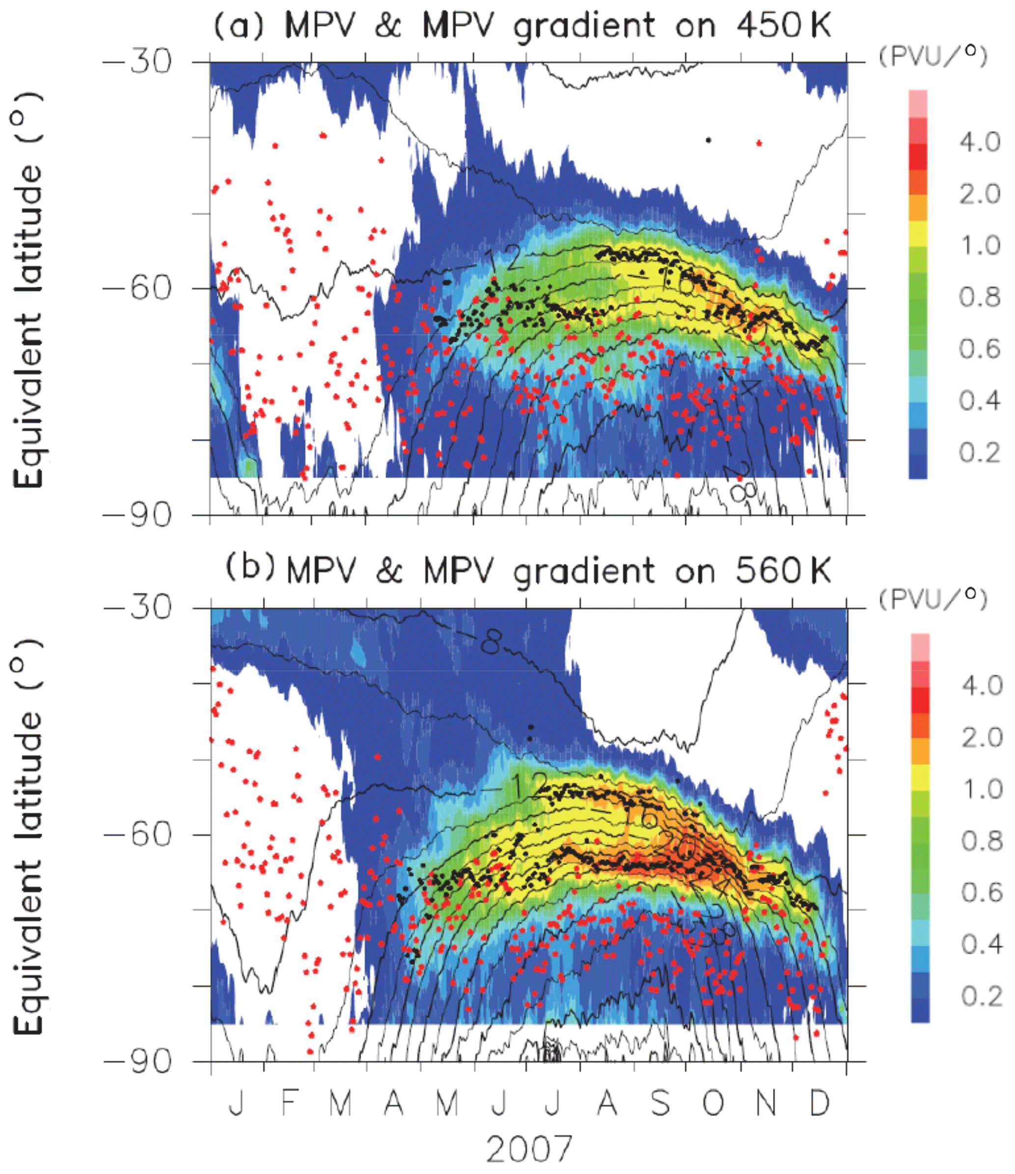
Figure B1 Time-equivalent latitude sections of MPV (contours) and its gradient with respect to EL (colors) at (a) 450 K and (b) 560 K isentropic PT surfaces in 2007. Black dots represent the inner and outer edge(s) of the polar vortex. Red dots represent the EL of Syowa Station on each day.

Figure B2 Same as Fig. B1 but for the year in 2011.

Appendix C: HCl null cycles (C₁ and C₂) and HCl destruction cycles (C₃ and C₄)

In Müller et al. (2018), new chemical cycles C₁ and C₂ were proposed to maintain high levels of active chlorine in the Antarctic spring, referred to as HCl null cycles, as follows:

$$\begin{array}{}\text{(R13)}& {\displaystyle }{\mathrm{CH}}_{\mathrm{4}}+\mathrm{Cl}\to \mathrm{HCl}+{\mathrm{CH}}_{\mathrm{3}},\text{(R21)}& {\displaystyle }{\mathrm{CH}}_{\mathrm{3}}+{\mathrm{O}}_{\mathrm{2}}+M\to {\mathrm{CH}}_{\mathrm{3}}{\mathrm{O}}_{\mathrm{2}}+M,\text{(R22)}& {\displaystyle }{\mathrm{CH}}_{\mathrm{3}}{\mathrm{O}}_{\mathrm{2}}+\mathrm{ClO}\to {\mathrm{CH}}_{\mathrm{3}}\mathrm{O}+\mathrm{Cl}+{\mathrm{O}}_{\mathrm{2}},\text{(R23)}& {\displaystyle }{\mathrm{CH}}_{\mathrm{3}}\mathrm{O}+{\mathrm{O}}_{\mathrm{2}}\to {\mathrm{HO}}_{\mathrm{2}}+{\mathrm{CH}}_{\mathrm{2}}\mathrm{O},\text{(R24)}& {\displaystyle }\mathrm{ClO}+{\mathrm{HO}}_{\mathrm{2}}\to \mathrm{HOCl}+{\mathrm{O}}_{\mathrm{2}},\text{(R4)}& {\displaystyle }\mathrm{HOCl}+\mathrm{HCl}\to {\mathrm{Cl}}_{\mathrm{2}}+{\mathrm{H}}_{\mathrm{2}}\mathrm{O},\text{(R5)}& {\displaystyle }{\mathrm{Cl}}_{\mathrm{2}}+h\mathit{\nu }\to \mathrm{2}\mathrm{Cl},\text{(R8)}& {\displaystyle }\mathrm{Cl}+{\mathrm{O}}_{\mathrm{3}}\to \mathrm{ClO}+{\mathrm{O}}_{\mathrm{2}}(\mathrm{2}\times ),\text{(R25)}& {\displaystyle }\mathrm{Net}\left({\mathrm{C}}_{\mathrm{1}}\right){\mathrm{CH}}_{\mathrm{4}}+\mathrm{2}{\mathrm{O}}_{\mathrm{2}}\to {\mathrm{CH}}_{\mathrm{2}}\mathrm{O}+{\mathrm{H}}_{\mathrm{2}}\mathrm{O}+\mathrm{2}{\mathrm{O}}_{\mathrm{2}},\text{(R26)}& {\displaystyle }{\mathrm{CH}}_{\mathrm{2}}\mathrm{O}+\mathrm{Cl}\to \mathrm{HCl}+\mathrm{CHO},\text{(R27)}& {\displaystyle }\mathrm{CHO}+{\mathrm{O}}_{\mathrm{2}}\to \mathrm{CO}+{\mathrm{HO}}_{\mathrm{2}},\text{(R24)}& {\displaystyle }\mathrm{ClO}+{\mathrm{HO}}_{\mathrm{2}}\to \mathrm{HOCl}+{\mathrm{O}}_{\mathrm{2}},\text{(R4)}& {\displaystyle }\mathrm{HOCl}+\mathrm{HCl}\to {\mathrm{Cl}}_{\mathrm{2}}+{\mathrm{H}}_{\mathrm{2}}\mathrm{O},\text{(R5)}& {\displaystyle }{\mathrm{Cl}}_{\mathrm{2}}+h\mathit{\nu }\to \mathrm{2}\mathrm{Cl},\text{(R8)}& {\displaystyle }\mathrm{Cl}+{\mathrm{O}}_{\mathrm{3}}\to \mathrm{ClO}+{\mathrm{O}}_{\mathrm{2}},\text{(R28)}& {\displaystyle }\mathrm{Net}\left({\mathrm{C}}_{\mathrm{2}}\right){\mathrm{CH}}_{\mathrm{2}}\mathrm{O}+{\mathrm{O}}_{\mathrm{3}}\to \mathrm{CO}+{\mathrm{H}}_{\mathrm{2}}\mathrm{O}+{\mathrm{O}}_{\mathrm{2}},\end{array}$$

Also, other chemical cycles which are responsible for the decline of HCl during Antarctic August and September, referred to as HCl destruction cycles, are also proposed by Müller et al. (2018) as follows:

$$\begin{array}{}\text{(R29)}& {\displaystyle }{\mathrm{CH}}_{\mathrm{2}}\mathrm{O}+h\mathit{\nu }\to \mathrm{CHO}+\mathrm{H},\text{(R30)}& {\displaystyle }\mathrm{H}+{\mathrm{O}}_{\mathrm{2}}+M\to {\mathrm{HO}}_{\mathrm{2}}+M,\text{(R27)}& {\displaystyle }\mathrm{CHO}+{\mathrm{O}}_{\mathrm{2}}\to \mathrm{CO}+{\mathrm{HO}}_{\mathrm{2}},\text{(R24)}& {\displaystyle }\mathrm{ClO}+{\mathrm{HO}}_{\mathrm{2}}\to \mathrm{HOCl}+{\mathrm{O}}_{\mathrm{2}}(\mathrm{2}\times ),\text{(R4)}& {\displaystyle }\mathrm{HOCl}+\mathrm{HCl}\to {\mathrm{Cl}}_{\mathrm{2}}+{\mathrm{H}}_{\mathrm{2}}\mathrm{O}(\mathrm{2}\times ),\text{(R5)}& {\displaystyle }{\mathrm{Cl}}_{\mathrm{2}}+h\mathit{\nu }\to \mathrm{2}\mathrm{Cl}(\mathrm{2}\times ),\text{(R8)}& {\displaystyle }\mathrm{Cl}+{\mathrm{O}}_{\mathrm{3}}\to \mathrm{ClO}+{\mathrm{O}}_{\mathrm{2}}(\mathrm{4}\times ),\text{(R31)}& {\displaystyle }\begin{array}{rl}\mathrm{Net}\left({\mathrm{C}}_{\mathrm{3}}\right)& {\mathrm{CH}}_{\mathrm{2}}\mathrm{O}+\mathrm{2}\mathrm{HCl}+\mathrm{4}{\mathrm{O}}_{\mathrm{3}}\\ & \to \mathrm{CO}+\mathrm{2}\mathrm{ClO}+\mathrm{2}{\mathrm{H}}_{\mathrm{2}}\mathrm{O}+\mathrm{4}{\mathrm{O}}_{\mathrm{2}},\end{array}\text{(R32)}& {\displaystyle }{\mathrm{O}}_{\mathrm{3}}+h\mathit{\nu }\to \mathrm{O}{(}^{\mathrm{1}}\mathrm{D})+{\mathrm{O}}_{\mathrm{2}},\text{(R33)}& {\displaystyle }\mathrm{O}{(}^{\mathrm{1}}\mathrm{D})+{\mathrm{H}}_{\mathrm{2}}\mathrm{O}\to \mathrm{2}\mathrm{OH},\text{(R34)}& {\displaystyle }\mathrm{OH}+{\mathrm{O}}_{\mathrm{3}}\to {\mathrm{HO}}_{\mathrm{2}}+{\mathrm{O}}_{\mathrm{2}}(\mathrm{2}\times ),\text{(R24)}& {\displaystyle }\mathrm{ClO}+{\mathrm{HO}}_{\mathrm{2}}\to \mathrm{HOCl}+{\mathrm{O}}_{\mathrm{2}}(\mathrm{2}\times ),\text{(R4)}& {\displaystyle }\mathrm{HOCl}+\mathrm{HCl}\to {\mathrm{Cl}}_{\mathrm{2}}+{\mathrm{H}}_{\mathrm{2}}\mathrm{O}(\mathrm{2}\times ),\text{(R5)}& {\displaystyle }{\mathrm{Cl}}_{\mathrm{2}}+h\mathit{\nu }\to \mathrm{2}\mathrm{Cl}(\mathrm{2}\times ),\text{(R8)}& {\displaystyle }\mathrm{Cl}+{\mathrm{O}}_{\mathrm{3}}\to \mathrm{ClO}+{\mathrm{O}}_{\mathrm{2}}(\mathrm{4}\times ),\text{(R35)}& {\displaystyle }\mathrm{Net}\left({\mathrm{C}}_{\mathrm{4}}\right)\mathrm{2}\mathrm{HCl}+\mathrm{7}{\mathrm{O}}_{\mathrm{3}}\to \mathrm{2}\mathrm{ClO}+{\mathrm{H}}_{\mathrm{2}}\mathrm{O}+\mathrm{9}{\mathrm{O}}_{\mathrm{2}}.\end{array}$$