the Creative Commons Attribution 4.0 License.
the Creative Commons Attribution 4.0 License.
 | 02 Aug 2019
Variations in the vertical profile of ozone at four high-latitude Arctic sites from 2005 to 2017
Shima Bahramvash Shams
Von P. Walden
Irina Petropavlovskikh
David Tarasick
Rigel Kivi
Samuel Oltmans
Bryan Johnson
Patrick Cullis
Chance W. Sterling
Laura Thölix
Quentin Errera
Understanding variations in atmospheric ozone in the Arctic is difficult because there are only a few long-term records of vertical ozone profiles in this region. We present 12 years of ozone profiles from February 2005 to February 2017 at four sites: Summit Station, Greenland; Ny-Ålesund, Svalbard, Norway; and Alert and Eureka, Nunavut, Canada. These profiles are created by combining ozonesonde measurements with ozone profile retrievals using data from the Microwave Limb Sounder (MLS). This combination creates a high-quality dataset with low uncertainty values by relying on in situ measurements of the maximum altitude of the ozonesondes (∼30 km) and satellite retrievals in the upper atmosphere (up to 60 km). For each station, the total column ozone (TCO) and the partial column ozone (PCO) in four atmospheric layers (troposphere to upper stratosphere) are analyzed. Overall, the seasonal cycles are similar at these sites. However, the TCO over Ny-Ålesund starts to decline 2 months later than at the other sites. In summer, the PCO in the upper stratosphere over Summit Station is slightly higher than at the other sites and exhibits a higher standard deviation. The decrease in PCO in the middle and upper stratosphere during fall is also lower over Summit Station. The maximum value of the lower- and middle-stratospheric PCO is reached earlier in the year over Eureka. Trend analysis over the 12-year period shows significant trends in most of the layers over Summit and Ny-Ålesund during summer and fall. To understand deseasonalized ozone variations, we identify the most important dynamical drivers of Arctic ozone at each level. These drivers are chosen based on mutual selected proxies at the four sites using stepwise multiple regression (SMR) analysis of various dynamical parameters with deseasonalized data. The final regression model is able to explain more than 80 % of the TCO and more than 70 % of the PCO in almost all of the layers. The regression model provides the greatest explanatory value in the middle stratosphere. The important proxies of the deseasonalized ozone time series at the four sites are tropopause pressure (TP) and equivalent latitude (EQL) at 370 K in the troposphere, the quasi-biennial oscillation (QBO) in the troposphere and lower stratosphere, the equivalent latitude at 550 K in the middle and upper stratosphere, and the eddy heat flux (EHF) and volume of polar stratospheric clouds throughout the stratosphere.
- Article
(5193 KB) - Full-text XML
-
Supplement
(7449 KB) - BibTeX
- EndNote


There is great interest in atmospheric ozone globally since the inception of the Montreal Protocol in 1987. Various parameters influence atmospheric ozone concentrations, including dynamical variability (Fusco and Salby, 1999; Holton et al., 1995; Kivi et al., 2007; Rao et al., 2004; Rex, 2004) and photolysis involving photochemical reactions (Yang et al., 2010) and climate variables (Rex, 2004). Studies show that the mean total column ozone (TCO) decreased from 1997 to 2003 globally (e.g., Newchurch, 2003), but some reports show that the rate of ozone depletion has recently decreased due to the ramifications of the Montreal Protocol (Weatherhead and Andersen, 2006; WMO, 2014; Steinbrecht et al., 2017; Weber et al., 2018). However, recent work shows evidence of decreases in lower-stratospheric ozone from 1998 to 2016 over 60∘ N to 60∘ S (Ball et al., 2018). Because of these changes, it is important to monitor ozone variability at many locations globally and to understand the causes of the variability.
During winters with persistent westerly zonal winds over the tropics, planetary-scale Rossby waves modulate stratospheric circulation. Stratospheric circulation is related to the tropical quasi-biennial oscillation (QBO; Ebdon, 1975; Holton and Tan, 1980). The interactions of planetary-scale Rossby waves and the QBO in the stratosphere modulate a meridional mass circulation towards the polar regions called the Brewer–Dobson circulation (Lindzen and Holton, 1968; Holton and Lindzen, 1972; Wallace, 1973; Holton et al., 1995). The location of the zero-wind line (latitude where the zonal wind speed is zero relative to the ground) is an important indicator of the strength of this circulation (Holton and Lindzen, 1972; Holton and Tan, 1980). During the easterly phase of the QBO, the zero-wind line shifts north, facilitating the propagation of planetary waves into the Arctic polar vortex. This creates a weakening of the vortex that increases the transport of relatively warm, ozone-rich air into the Arctic (Holton and Tan, 1982). The warmer temperatures are associated with decreased occurrence of polar stratospheric clouds (PSCs) and consequently fewer heterogeneous reactions involving the PSCs, which lead to less photochemical ozone loss in the stratosphere (Rex, 2004; Shepherd, 2008). Conversely, during the westerly phase of the QBO, the propagation of planetary waves between the tropics and the Arctic decreases, and the polar vortex is strengthened, resulting in lower temperatures and increased probability of photochemical ozone loss. Thus, dynamical processes and the state of the polar vortex are important factors that determine ozone amounts in the Arctic.
Although there is strong observational evidence to support this teleconnection between the tropical and Arctic atmosphere, a complete theoretical explanation has proved difficult (Anstey and Shepherd, 2014). The interaction of the background zonal mean wind and planetary waves is not completely understood, which makes it difficult to ascribe, in detail, how atmospheric dynamics affect the polar vortex. Furthermore, these effects depend on location and can also affect different portions of the atmosphere (Staehelin et al., 2001; Rao, 2003; Rao et al., 2004; Yang et al., 2006; Vigouroux et al., 2008, 2015). Thus, detailed analyses of the vertical structure of ozone are needed at various locations to fully understand the variability in ozone concentrations. This situation is exacerbated by both the lack of high temporal observations at high latitudes as well as the difficulty of making quality measurements during winter; many ground-based and spaceborne remote-sensing instruments for measuring ozone depend on solar radiation (Bowman, 1989; Hasebe, 1980; Vigouroux et al., 2008, 2015). The Microwave Limb Sounder (MLS) is a spaceborne instrument that measures atmospheric emission, which makes it capable of retrieving ozone over the Arctic (Waters et al., 2006). This capability motivates the use of MLS retrievals for analysis of stratospheric ozone in the Arctic (Manney et al., 2011; Kuttippurath et al., 2012; Wohltmann et al., 2013; Livesey et al., 2015; Strahan and Douglass, 2018).
One of the most important and reliable instruments for measuring the vertical profile of ozone is the ozonesonde. These instruments can be launched year-round and can provide valuable information for the validation of remote-sensing instruments aboard satellites. The Global Monitoring Division (GMD) of the National Oceanic and Atmospheric Administration (NOAA), Environment and Climate Change Canada, and the Helmholtz Centre for Polar and Marine Research launch ozonesondes routinely in the Arctic. Ozonesondes have used the data to study trends, patterns, and the vertical distribution of ozone from many locations (Logan, 1994; Steinbrecht et al., 1998; Logan et al., 1999; Solomon et al., 2005; Miller et al., 2006). Ozonesonde profiles from various Arctic stations have been used to study the climatology of the ozone cycle (Rao et al., 2004), the vertical distribution of ozone and its dependence on different proxies (Rao, 2003; Tarasick, 2005; Kivi et al., 2007; Gaudel et al., 2015), trends and annual cycles of ozone (Christiansen et al., 2017), the variability in ozone due to climate change (Rex, 2004), ozone loss and the relation to dynamical parameters (Harris et al., 2010), and the difference of ozone depletion in the Arctic and Antarctic (Solomon et al., 2014) and to validate other sensor measurements (McDonald et al., 1999; Vigouroux et al., 2008; Ancellet et al., 2016).
The sector of the Arctic from 0 to 60∘ W is known to be very sensitive to dynamical processes (see Fig. 2a of Antsey and Shepherd, 2014). In spite of this, the long record of ozonesonde launches (2005–2017) by NOAA GMD has never been used to study the long-term variability in tropospheric and stratospheric ozone over Summit Station, Greenland (72.6∘ N, 38.4∘ W; 3200 m). Summit Station is located in central Greenland atop the Greenland ice sheet (GrIS) and is the drilling site of the Greenland Ice Sheet Project 2 (GISP2) ice core. Ny-Ålesund, Svalbard, Norway, and Alert and Eureka, Nunavut, Canada, are high-latitude stations in this section of the Arctic that also routinely launch ozonesondes.
In this study, we use 12 years of ozonesonde measurements (from 2005 to 2017) to document the vertical structure of ozone at high-latitude sites in the Arctic. In Sect. 2, we describe how ozone profiles over these sites are constructed using data from both ozonesondes and satellite retrievals from the MLS. This section also describes the data screening that was performed on these measurements. Section 3 discusses the methods used in the data analysis, including determination of the seasonal cycle and the stepwise multiple regression (SMR) technique (Appenzeller et al., 2000; Brunner et al., 2006; Kivi et al., 2007; Vigouroux et al., 2015; Steinbrecht et al., 2017). Stepwise multiple regression is used to determine the drivers of ozone variations at each of the sites. Section 4 presents the results of this study, including the seasonal cycles, trends, and variations in total column ozone (TCO) and partial column ozone (PCO) in four atmospheric layers: the troposphere and the lower, middle, and upper stratosphere. This section also determines the important drivers of the deseasonalized ozone data (based on various proxies using stepwise multiple regression) that are common to all of the four sites. These drivers are then used to create final models of ozone variations. Section 5 presents the conclusions of this research study.
Summit Station, Greenland (72∘ N, 39∘ W); Ny-Ålesund, Svalbard, Norway (79∘ N, 12∘ E); Alert, Canada (82∘ N, 62∘ W; and Eureka, Canada (70∘ N, 86∘ W), are chosen as the study sites for this research because there is a long history of ozonesonde observations at these locations. Figure 1 shows the locations of these stations in the Arctic.
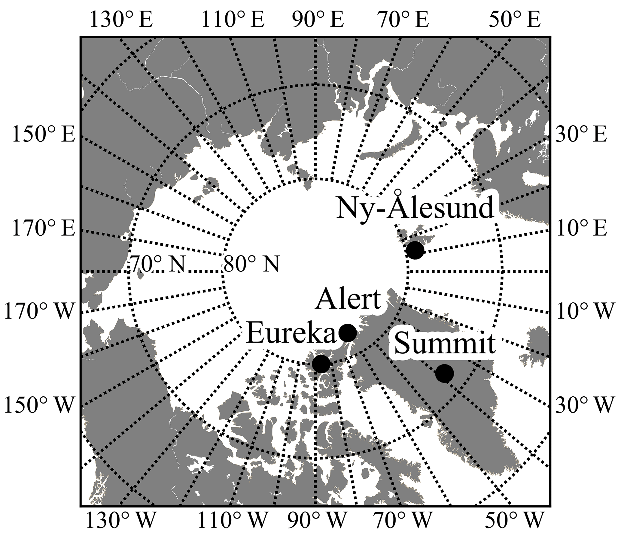
Figure 1Map showing the locations of study sites used: Summit Station, Greenland; Ny-Ålesund, Svalbard, Norway; Alert, Nunavut, Canada; and Eureka, Nunavut, Canada.
Summit Station ozone measurements were started in February 2005 and continued until the summer of 2017. The other stations have longer datasets, but in this study, 12 annual cycles from February 2005 through February 2017 are studied to have a consistent dataset at all stations. The time period is also constrained by the availability of MLS data, which have been available since 2004. The ozonesonde profiles from Summit Station are available from NOAA's Earth System Research Laboratory, while the profiles from the Canadian stations and Ny-Ålesund can be found at the World Ozone and Ultraviolet Radiation Data Centre (WOUDC). The ozonesondes used here utilize electrochemical concentration cells (ECCs; Komhyr, 1969), manufactured by either Science Pump for Ny-Ålesund or Environmental Science (EN-SCI) for Summit, Alert, and Eureka. The ozonesondes at Ny-Ålesund, Alert, and Eureka used a sensing solution of neutral buffered 1 % potassium iodide, while the ozonesondes at Summit used a reduced (one-tenth) buffer concentration. The data records of the Canadian sites have recently been re-evaluated (Tarasick et al., 2016), as has the Summit record (Sterling et al., 2018). Based on the ozone sensor response time of 25–40 s (Smit and Kley, 1998), and assuming a typical balloon ascent rate of 4–5 m s−1, the ozonesondes have a vertical resolution of about 100–200 m. The measurement precision is ±3 %–5 %, and the overall uncertainty in ozone concentration in parts per million volume is from about ±10 % up to 30 km (Komhyr, 1986; Komhyr et al., 1989; Kerr et al., 1994; Johnson et al., 2002; Smit et al., 2007; Deshler et al., 2008, 2017).
We use retrievals from the MLS (version 4.2) above the maximum height of each ozonesonde up to 60 km. The MLS is an instrument on the Aura spacecraft that uses microwave emission to measure atmospheric composition, temperature, and cloud properties (Waters et al., 2006). Ozone retrievals from the MLS have been available continuously since 2004 over the Arctic, with overpasses over these sites every few days. The standard MLS ozone product, which is retrieved from spectra with frequency 240 GHz, is used in this study. The column value uncertainty (σ) is 2 % to 3 % (Livesey et al., 2018). The vertical resolution of the MLS profiles is from 100 to 22 hPa is 2.5 km and increases to 3 km in both the lower and upper stratosphere (Livesey et al., 2017). The MLS ozone products have previously been used in ozone analyses, e.g., for polar ozone loss (Manney et al., 2011; Kuttippurath et al., 2012; Wohltmann et al., 2013; Livesey et al., 2015; Strahan and Douglass, 2018).
Data screening was performed on each ozonesonde used in this study. Figure 2 shows a histogram of the maximum height of the ozonesondes for the entire 12-year period at all study locations. Most of the ozone profiles have maximum heights of 25 km or greater, but there is a significant fraction with maximum heights below 25 km. A bi-modal distribution is apparent at all stations except Ny-Ålesund and is caused partly by the fact that the burst altitude of the balloons depends on season; lower maximum altitudes are achieved in the extreme cold experienced during winter. The MLS has high uncertainty in the lower atmosphere. Thus, to minimize the uncertainty in the calculation of TCO, ozonesondes that reached a maximum height of greater than 12 km were used in this study; profiles with maximum heights below 12 km were eliminated from further analysis. The fraction of TCO below 12 km (∼200 hPa) at these sites is about 13 %–17 %.
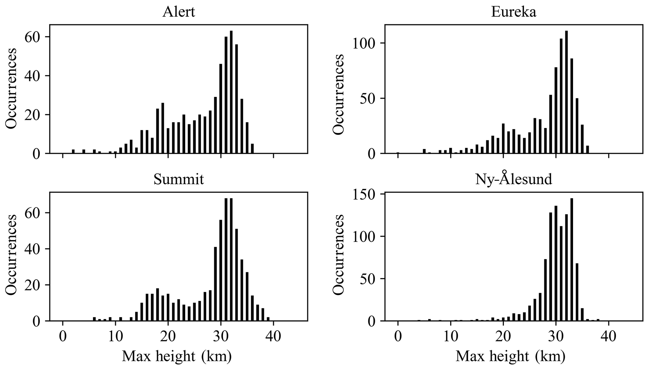
Figure 2Maximum height reached by ozonesondes launched at Alert, Nunavut, Canada; Eureka, Nunavut, Canada; Summit Station, Greenland; and Ny-Ålesund, Svalbard, Norway, between February 2005 and February 2017.
Another data-screening issue is related to missing data in the ozonesonde profiles. Most of the missing values occur at high altitudes because the ozonesonde ceased to report valid measurements. There were also some missing data between valid ozone measurements. In this study, profiles that have a percentage of missing data greater than 40 % are eliminated from further analysis. In the remaining profiles, if missing values occurred between valid ozone measurements, the profile was linearly interpolated to fill the missing data. After applying the data screening, more than 25 ozonesondes are retained for analysis in each month for the 12-year period, which satisfies the requirement for calculating a meaningful monthly mean profile (Logan et al., 1999).
Ozone profiles in this study are constructed by merging the ozonesondes up to the burst altitude (Fig. 2) and then using the MLS profiles up to 60 km. The merged profiles are generated only if an MLS ozone profile is within a 2∘×2∘ latitude–longitude grid cell around each station and within 4 d of the ozonesonde launch. The majority of the merged profiles are generated using MLS data on the day of the launch or within 1 d of the launch. Figure 3 shows the difference of TCO from the merged ozone profile versus TCO from the MLS only at all stations. This shows that the MLS mostly overestimates the ozone in the lower atmosphere at all stations. Thus, the merged profile dataset minimizes the uncertainty in ozone at these sites by using the more accurate ozonesonde data for as much of the lower atmosphere as possible.
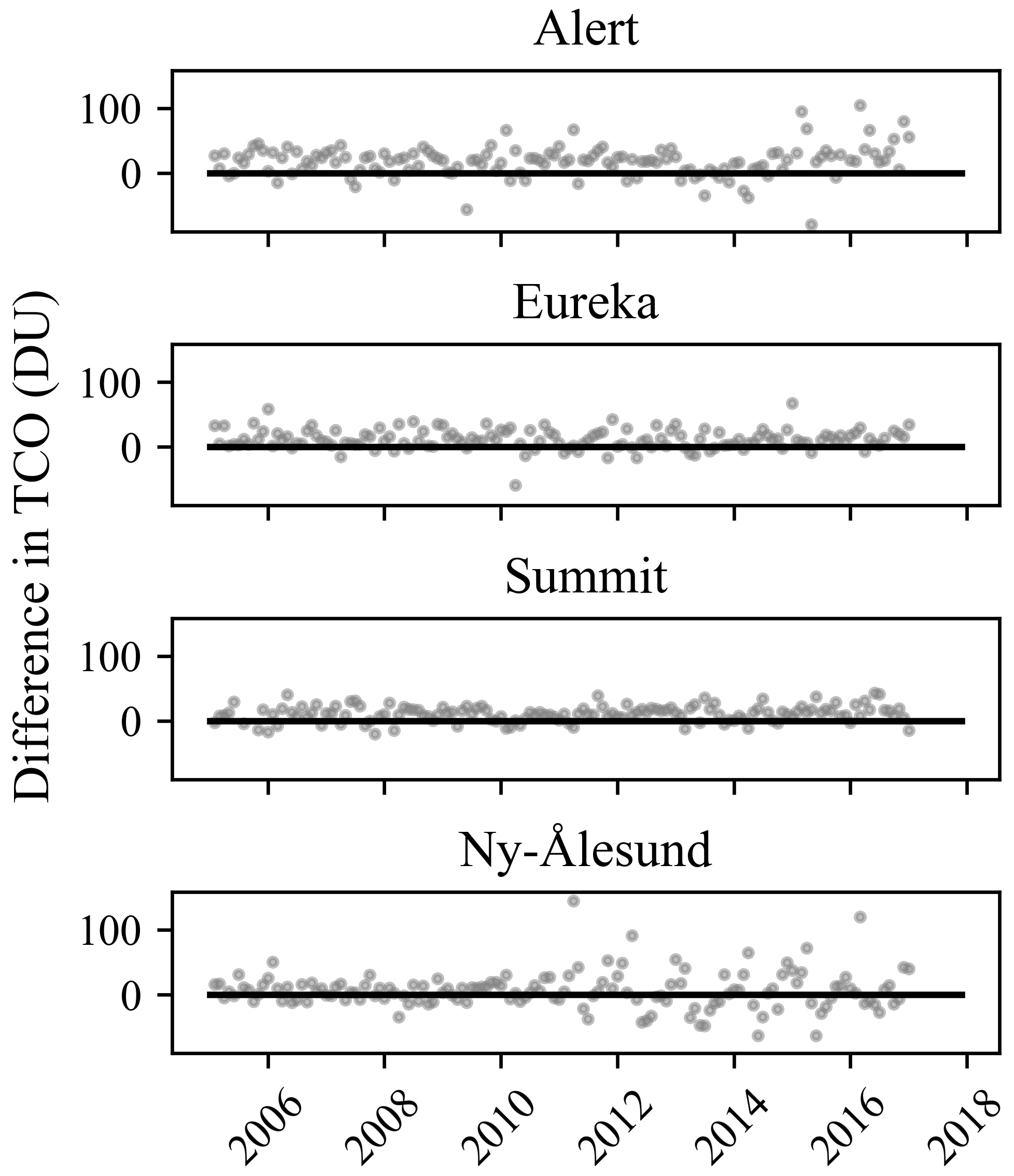
Figure 3The difference in total column ozone (TCO) calculated using profiles from the Microwave Limb Sounder (MLS) only versus profiles using ozonesonde in the lower atmosphere and MLS in the upper atmosphere. The differences are calculated as MLS only minus the ozonesonde and MLS for Alert, Eureka, Summit, and Ny-Ålesund.
The total amount of ozone in the vertical profile is a useful parameter for understanding ozone variations in the atmosphere. The ozone column density is traditionally defined by the Dobson unit (DU), which is the thickness of a compressed gas in the atmospheric profile in units of 10 µm at standard temperature and pressure; 1 DU is equivalent to 1 milli-atmosphere centimeter or 2.69×10¹⁶ molecules cm−2. Merged ozonesondes up to 60 km provide an appropriate dataset to integrate over all layers of the atmosphere that contain appreciable ozone. In this study, the PCO amounts are calculated for the following altitude regions: surface to 10, 10 to 18, 18 to 27, and 27 to 60 km. For the purpose of this study, the layers represent the troposphere, lower stratosphere, middle stratosphere, and upper stratosphere, respectively. Note that the tropopause is low in the Arctic, so the layer from the ground to 10 km represents primarily values in the troposphere but also contains some ozone from the lowest portion of the stratosphere. However, we refer to this layer here as the “troposphere” for convenience.
SMR has been widely used in the past (e.g., Appenzeller et al., 2000; Brunner et al., 2006; Kivi et al., 2007; Mäder et al., 2007; Vigouroux et al., 2015) for selecting important variables that affect ozone concentrations. Wohltmann et al. (2007) explain some of the issues with using multiple regression to determine atmospheric ozone variations. However, this technique can be inaccurate if there is spurious correlation between the different variables and the deseasonalized ozone time series (Wohltmann et al., 2007). In this study, we use a combination of SMR and the “process-based” approach of Wohltmann et al. (2007) to determine the important drivers of ozone variations at the Arctic sites. In particular, SMR is used to determine a set of physical parameters that are important at three or more of the sites and are, therefore, common drivers of ozone variations in the Arctic. These variables are then used to derive final models for PCO in each of the four atmospheric layers and for TCO at each site. This procedure then reduces the effect of spurious correlations between variables and deseasonalized ozone time series that is experienced when using SMR only.
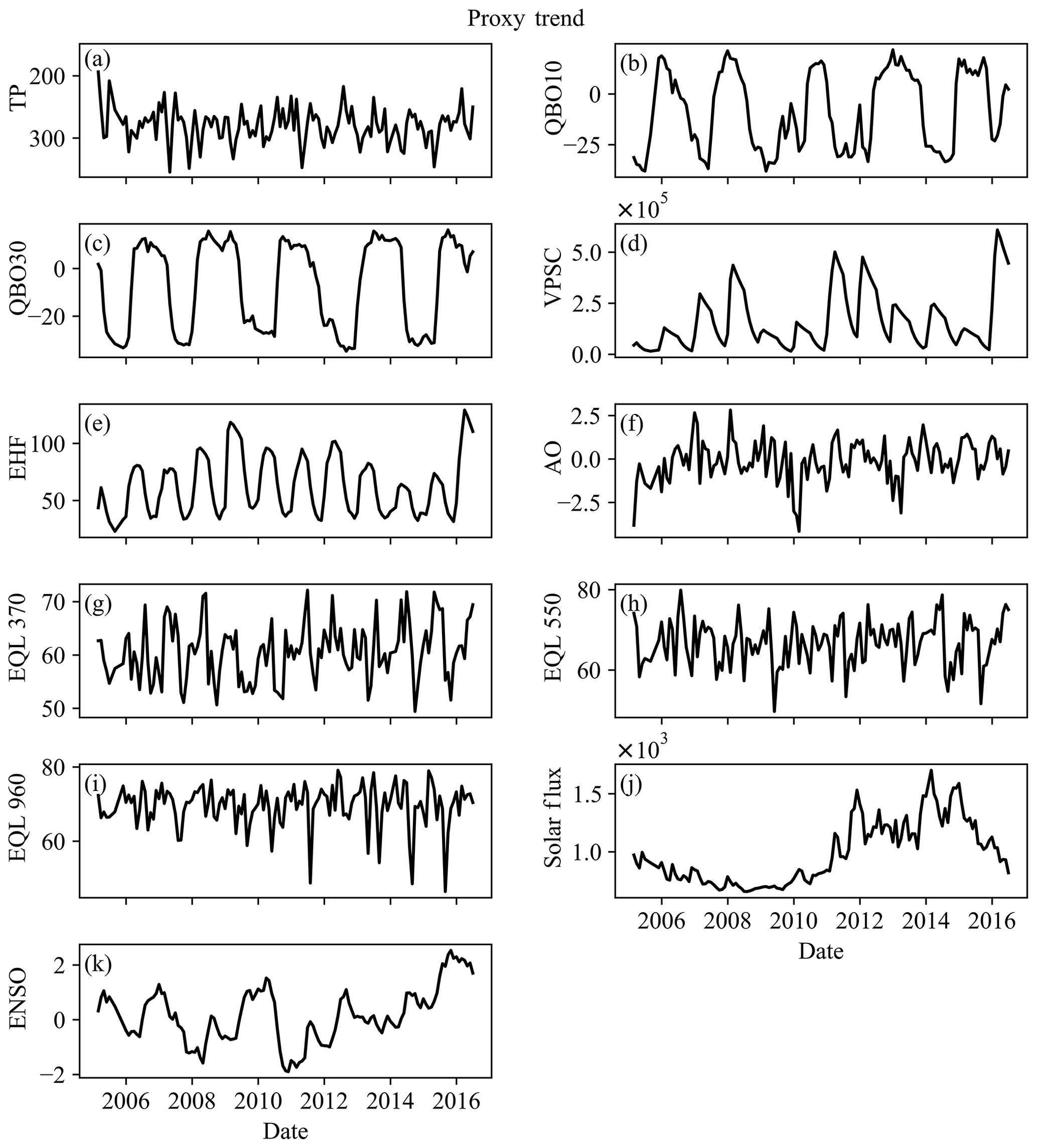
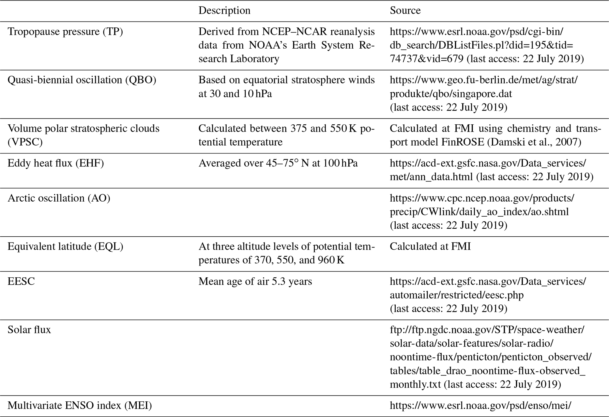
Figure 4Time series of the proxies used in this study to analyze ozone variations over Summit Station, Greenland. The sources of the proxies are listed in Table 1. The units of the proxies are unitless for ENSO and AO; meters per second for QBO10 and QBO30 (positive values are westerly zonal winds, and negative values are easterlies), watts per square meter for solar flux and eddy heat flux (EHF), hectopascals for tropopause pressure (TP), 106 km3 for volume of polar stratospheric clouds (VPSC), and degrees for equivalent latitude (EQL) at potential temperatures of 370, 550, and 960 K. The proxy for VPSC is actually the cumulative volume of polar stratospheric clouds times the effective equivalent stratospheric chlorine (EESC), and cumulative EHF is named EHF (Brunner et al., 2006), as explained in the text. The proxies for TP and EQL are for Summit Station.
The general approach is briefly explained here, while the analysis and results are discussed below in Sect. 4. First, the SMR uses various proxies that have been previously identified as important indicators of ozone concentrations in the troposphere and stratosphere. Figure 4 shows time series of the proxies: tropopause pressure (TP); the QBO at both 10 and 30 hPa (QBO10; QBO30); the volume of polar stratospheric clouds (VPSC); eddy heat flux (EHF); Arctic oscillation (AO); equivalent latitude (EQL) at three potential temperature levels, 370, 550, and 960 K; solar flux (SF); and the El Niño–Southern Oscillation index (ENSO). The monthly averaged values for TP and AO are calculated using data for the same dates as the ozonesonde launches for each station. EQL, TP, and AO are estimated at each station. In Fig. 4, EQL, TP, and AO at Summit Station are shown as examples. Table 1 lists the data sources and weblinks of these proxies. This list is similar to that used by previous studies (Brunner et al., 2006; Vigouroux et al., 2015). Following Vigouroux et al. (2015), the stepwise multiple regression model is given by
where Y(t) is the final regression model, t is the month (1 to 12), A0–A4 are coefficients related to the seasonal cycle, Ak (for k≥5) is the coefficients related to the proxy time series X(t)k, and ε is the residual ozone that is not explained by the combination of the seasonal cycle and the proxies. Any linear trend in the data is considered to be one of the proxies using Xk(t)=t. The model is implemented using the following procedure. First, the seasonal cycle for the 12-year period is determined by finding the coefficients A0–A4. These terms are then subtracted from the original TCO time series to yield deseasonalized time series. Using the technique described in Sect. 7.4.2 of Wilks (2011), stepwise regression (with forward selection) is then performed on the deseasonalized time series using the different proxies. To accomplish this, each proxy is regressed with the deseasonalized TCO and PCO time series, and the proxy that has the highest explained variance (R2) and a p value lower than 0.05 is selected. This proxy (e.g., A5X5(t)) is then included in a new fit to the time series using multiple linear regression to create a new time series. This process is repeated until none of the remaining proxies increase the R2 by more than 1 %. The final set of drivers of Arctic ozone in each layer, as well as the TCO, are defined as those that are common among three or more sites, based on the SMR analysis. These proxies are then used to create a final model for PCO and TCO, as described in Sect. 4.4.
Table 1Proxies used in the stepwise multiple regression performed in this study to explain variance in the total column ozone amount.
In this section, the 12-year records of ozonesonde profiles over the four Arctic stations are discussed. First, the seasonal cycles of ozone at the four sites are compared. The trends of ozone in various vertical sections of the atmosphere are also discussed. Finally, we describe the results of the SMR analysis and the final ozone models, which yield insight into the primary drivers of ozone variability over four Arctic stations.
4.1 Seasonal cycle
To examine the seasonal cycle at each station, the monthly averaged TCO and PCO are calculated. The TCO (and the PCO amounts) depends on both temperature and pressure, so differences in the profiles of these variables over the different sites will affect the column ozone. Figure 5 shows the multi-year monthly averages (left column) and the associated standard deviations (right column) of TCO (top row) and the PCO amounts for the four atmospheric layers. The total column ozone reaches its peak value in April for all stations. The minimum value of TCO at all sites occurs in September or October. The ozone values in the upper stratosphere fluctuate between 40 and 80 DU for all stations. The largest values of PCO occur in the layers of the middle (120–160 DU) and lower stratosphere (75–150 DU). The PCO in the troposphere ranges from about 20 to 35 DU at Summit Station and from 35 to 50 DU at the other stations. These values are lower at Summit Station due to its high surface elevation of about 3200 m.
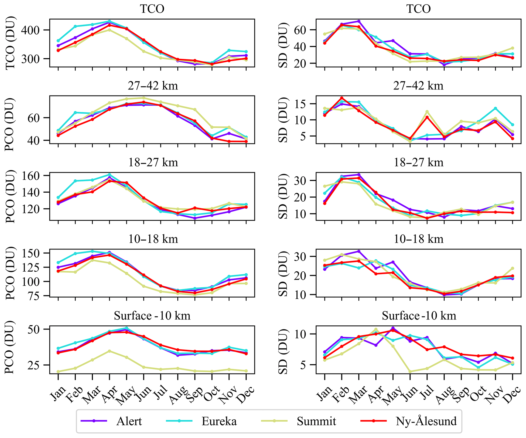
Figure 5Monthly mean (left panels) and standard deviations (right panels) of total column ozone (TCO) and partial column ozone (PCO) for 2005–2017 for different atmospheric layers from merged ozonesonde and MLS for Alert, Eureka, Summit, and Ny-Ålesund. The layers represent the troposphere (surface–10 km), the lower stratosphere (10–18 km), the middle stratosphere (18–27 km), and the upper stratosphere (27–42 km). The TCO is calculated from the surface to 60 km.
The seasonal cycles of TCO show significant differences at the four sites. The cycles at Alert and Eureka are similar, but Eureka exhibits slightly larger values than Alert from November to March. The differences between these two sites are somewhat surprising given the close proximity of the two stations. The TCO values at Ny-Ålesund are larger than any other site from May to August but then exhibit the lowest TCO in winter (November–January). The TCO values at Summit are the lowest of any of the sites in May, June, and July. The seasonal cycle of the standard deviations in the TCO are similar at all the sites, with maximum values in late winter and early spring and minimum values in fall.
The seasonal cycles are also quite different in the various atmospheric layers. The timing of the peak ozone at different altitudes is due to different physical processes that affect ozone concentrations. In the upper stratosphere (27–42 km), the values are about 30 to 40 DU higher in spring than the minimum in the fall due to increased sunlight in spring, when photolysis equilibrium is reached (Crutzen, 1971). For all stations, the PCO values in this layer peak later in the year than the TCO, with values of about 75–80 DU in May, June, and July. The PCO is slightly higher in most months at Summit Station compared to the other stations. The standard deviations in the upper stratosphere are similar at all stations, except for Summit and Ny-Ålesund, which have larger variability than Alert and Eureka in June.
The PCO in the middle stratosphere peaks earlier in spring than in the upper stratosphere, peaking in April at Alert, Eureka, and Summit and in May at Ny-Ålesund. Similar to the TCO, the PCO values at Ny-Ålesund remain elevated (relative to the other sites) through most of the summer until August. This springtime maximum is due to accumulation of transported ozone from lower latitudes during wintertime caused by the Brewer–Dobson circulation (Staehelin et al., 2001). The PCO is largest at Eureka from November to April. All stations show similar standard deviations in this layer, with the largest fluctuations in winter and spring.
The PCO in the lower stratosphere peaks in March at Summit Station and Eureka and in April at Ny-Ålesund and Alert. This pattern represents the well-known springtime maximum in the Arctic, which is caused by winter ozone accumulation that occurs before ozone is transported to the troposphere (Rao, 2003; Rao et al., 2004; Staehelin et al., 2001). Summit Station has lower PCO values in this layer from April to September. The springtime decline in ozone over Summit appears to start earlier (in March), and then the ozone remains low until October. The PCO at Ny-Ålesund has a large range, with minimum values similar to Summit Station in fall but maximum values due to wintertime accumulation that are similar to Alert and Eureka.
Eureka and Alert have very similar seasonal cycles of tropospheric ozone, reaching a maximum in May and minimum in August. On the other hand, the PCOs at Summit Station and Ny-Ålesund peak in April and June. As expected, the ozone fluctuations in this layer are small. In general, the standard deviations in tropospheric PCO are smallest at Summit Station, likely due to the lower PCO values. The peak in the tropospheric PCO in spring is caused primarily by relatively large ozone concentrations between 6 and 10 km. The peak in the upper troposphere is likely caused by intrusion of ozone-rich air from the stratosphere. The subsequent intrusion of ozone into the troposphere later in the spring is likely the result of tropospheric folds that occur in mid-spring to late spring (Holton et al., 1995; Walker et al., 2012; Tarasick et al., 2019).
4.2 Trends
The temporal trends in the TCO and PCO at all four stations are now considered. Linear regression is performed on the time series to determine the temporal trends. For a trend to be significant, the slope of the regression line must be greater than the standard error in the slope by 0.1 DU yr−1. The details of the trend analysis can be found in Figs. S1–S5 and Table S1 in the Supplement.
The trends were calculated for the 12-year period using annual, spring (MAM), summer (JJA), fall (SON), and winter (DJF) values. There is no significant trend in the annual values of the TCO or any of the PCO values at any of the stations. Ny-Ålesund and Summit Station are the only sites that have significant seasonal trends. In spring, Ny-Ålesund has a negative trend in both the troposphere ( DU yr−1) and the upper stratosphere ( DU yr−1). In summer, Summit has a negative trend in the upper stratosphere ( DU yr−1), and Ny-Ålesund has relatively large positive trends in the troposphere ( DU yr−1), lower stratosphere ( DU yr−1), middle stratosphere ( DU yr−1), and in the total column ( DU yr−1). In fall, Ny-Ålesund has significant trends in all the stratospheric layers, but the trend is positive in the upper stratosphere ( DU yr−1) and negative in the middle stratosphere ( DU yr−1) and the lower stratosphere ( DU yr−1). In fall, Summit exhibits negative trends in both the TCO ( DU yr−1) the middle stratosphere ( DU yr−1).
In summary, Alert and Eureka have no significant trends in ozone. There are a few significant trends at Summit Station in summer and fall that are all negative. Ny-Ålesund has trends in spring, summer, and fall, with the large positive trends in summer and mostly small negative trends in spring and fall.
4.3 Drivers of ozone variation over Greenland
To identify the drivers of ozone variations, the SMR technique described in Sect. 3 is used. We refer back to Fig. 4, which describes the proxies used for SMR. The most dominant source of ozone variation is the seasonal cycle, so the first step in the analysis is to remove this cycle. To remove the seasonal cycle, we first fit the TCO and PCO time series using the first five terms in Eq. (1) (using coefficients A0–A4). The derived seasonal cycle is then subtracted from the original time series to create a deseasonalized time series. Figure 6 shows the values of total column ozone (top panels) and the partial ozone column values for each of the four altitude regions (bottom four panels) for each station. The seasonal cycles are also shown in Fig. 6 as the green curves. The values of the correlation of determination (R2) are shown above each panel and represent the variance in the original time series that is explained by the seasonal cycle. These values are also shown in Table 2 for comparison. The seasonal cycle explains over 50 % of the variance in both the total and partial column ozone values at all stations except the middle stratosphere at Summit Station (47 %) and Ny-Ålesund (38 %). The R2 value for TCO is highest at Eureka (0.80) and lowest at Ny-Ålesund (0.65). Because the seasonal cycle explains a high percentage of the ozone fluctuations over Eureka, this site may be less susceptible to dynamical and chemical perturbations compared to the other sites. By comparing the R2 values in the different atmospheric layers, we see that the middle stratosphere has the lowest R2 at all the stations except Eureka. This shows that the ozone in the middle stratosphere at these Arctic sites is more susceptible to perturbations than other layers.
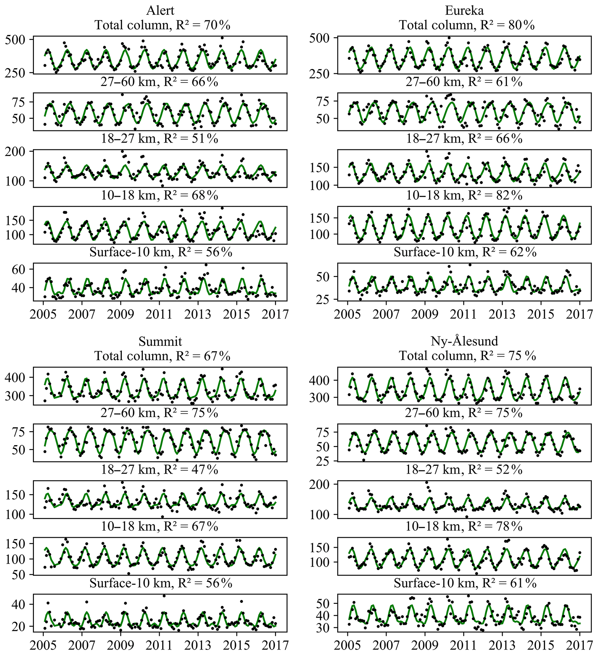
Figure 6Time series of the total column ozone (top panels) and the partial column ozone (black dots) in four atmospheric layers (four bottom panels) from Alert, Eureka, Summit, and Ny-Ålesund. The fitted seasonal cycle is shown as the green curves. The coefficient of determination (R2) for each seasonal fit is shown in the title for each panel.
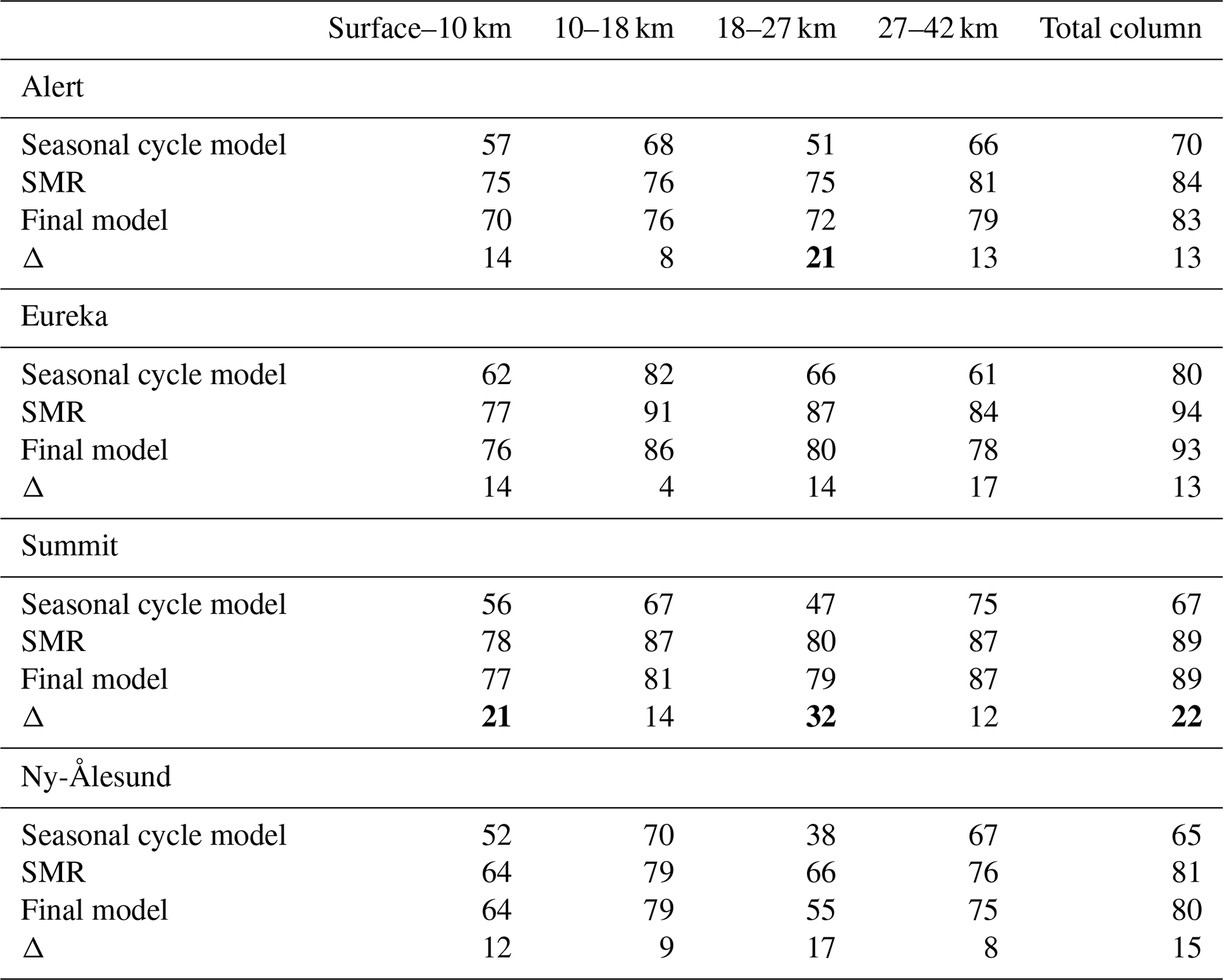
Table 2Correlation of determination (R2 in %) for the seasonal cycle, stepwise regression model (SMR), and the final model of ozone variations (February 2005–February 2017). The improvement in the correlation of determination between the seasonal cycle and final models is shown as Δ for each station. The text is in bold when the improvement is higher than 20 %.
By examining the difference between the original time series (black dots) and the seasonal cycles (green lines) in Fig. 6, we can see that there is additional variance that remains unexplained. This is motivation to conduct the SMR analysis to identify the most important drivers that are common at the four Arctic sites. To accomplish this, the SMR analysis is performed on the deseasonalized time series. Before the results of the SMR analysis are discussed, it is important to note that the removal of the seasonal cycle likely decreases the influence of proxies that have seasonal variations. Figure 4 shows that this is mostly true for the eddy heat flux and, to a lesser degree, the volume of polar stratospheric clouds.
The SMR analysis is initiated by calculating the coefficient of determination (R2) for each proxy. The best proxy at each step in the analysis is the one with the largest R2 value, which is at least 1 % higher than the R2 of the previous step. These fits must also have a p value of less than 0.05 to be considered in the analysis. Table 3 summarizes the results for each time series. (More detailed information, such as the regression slopes and standard errors of the slope, can be found in Tables S2–S5 of the Supplement.) The lists of proxies are in descending order of contribution to the correlation of determination. We also list the sign of the slope of the regression fit of each proxy in Table 3 to the left of the R2 value (except for the QBO because this proxy involves multiple terms); the sign of the slope indicates positive or negative correlation between the proxy and the deseasonalized time series. The bottom row of Table 3 lists the cumulative R2 value of all selected proxies. The time trends were included in the regression analysis by using Ak=1 in Eq. (1).
Table 3The correlation of determination (R2 in %) obtained in the stepwise multiple regression analysis. The regression is performed on the deseasonalized ozone time series. The R2 values are listed in order of improvement in the descending order. Proxies that improve the R2 by at least 1 % and that have a p value equal or less than 0.05 are added to model. The sign next to the R2 value is the sign of the slope of the regression. The R2 of the final residual model for each atmospheric layer is shown in the bottom row. The sign of the QBO is not shown because its contribution comes from several different terms, and a single slope sign is thus not applicable for this proxy. Extended tables for each station can be found in the Supplement.
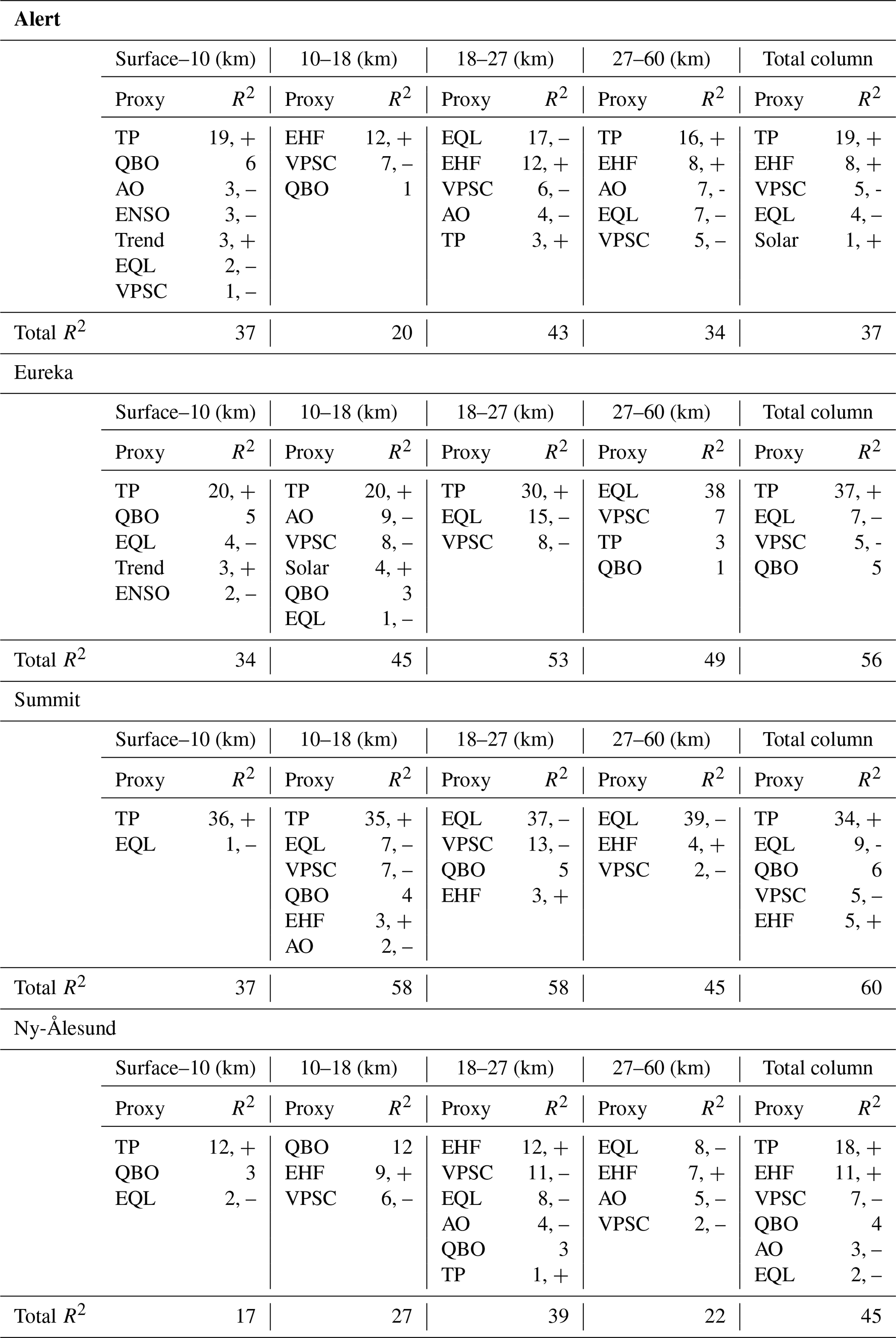
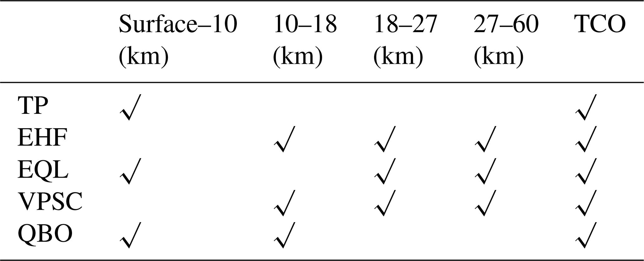
To identify the most important proxies that affect Arctic ozone (to be used in our final model), we use proxies that are selected at three or more of the four sites. Table 4 shows that tropopause pressure (TP) is the most important proxy for TCO and tropospheric PCO at all of the stations. The seasonal cycle in TP is difficult to detect in Fig. 4a, but the largest values of TP generally occur in winter and spring; note that the y axis in Fig. 4a decreases upward, so large pressure values indicate lower height levels in the atmosphere. TP has been shown to correlate well with total column ozone (Appenzeller et al., 2000; Steinbrecht et al., 1998). Lower TP (higher tropopause height) leads to lower values of ozone (Steinbrecht et al., 1998). Tropopause height can also be increased due to lower stratosphere temperatures (Forster and Shine, 1997), which can result in ozone depletion (Rex, 2004). The transport of ozone to higher levels in the atmosphere can increase ozone destruction because photochemical reactions increase (when sunlight is available; Steinbrecht et al., 1998).
Table 4The important drivers of ozone variations for each atmospheric layer and for total column ozone (TCO). The drivers are tropopause pressure (TP), eddy heat flux (EHF), equivalent latitude (EQL), volume of polar stratospheric clouds (VPSC), and the quasi-biennial oscillation (QBO). The EQL at 370 K is used for surface to 10 km, and the EQL at 550 K is used for the middle and upper stratosphere.
Potential vorticity (PV) also affects the ozone concentration. Equivalent latitude (EQL) is an index estimated based on PV that is indicative of ozone (air parcel) transportation on an isentropic level of potential temperature (Danielsen, 1968; Butchart and Remsberg, 1986; Allen and Nakamura, 2003). Adiabatic vertical movement of air parcels, caused by stratosphere–troposphere transport, changes the volume of an air parcel. The mixing ratio is conserved in adiabatic movement; thus this transportation changes the density of ozone (Wohltmann et al., 2005). Moreover, horizontal advection on isentropic levels can affect the ozone concentration when there is an ozone gradient (Allen and Nakamura, 2003, Wohltmann et al., 2005). We use equivalent latitude at three potential temperature levels of 370, 550, and 960 K. Monthly fluctuations of these levels are shown in Fig. 4g, h, and i. The EQL at 550 K significantly influences Arctic ozone variations in the middle and upper stratosphere, while the EQL at 370 K is found to have an important influence on tropospheric ozone at these sites.
The Brewer–Dobson circulation is one of the most important processes of ozone transport from the tropics to the Arctic (Staehelin et al., 2001). The seasonal cycle of ozone in the extratropics is caused by this circulation (Fusco and Salby, 1999). The vertical component of the Eliassen–Palm (EP) flux and the EHF are proportional to each other and are both good indicators of the Brewer–Dobson circulation (Brunner et al., 2006; Eichelberger, 2005; Fusco and Salby, 1999). In this study, the spatially averaged EHF at 100 hPa over 45–75∘ N is used. The variation in EHF is shown in Fig. 4e. As mentioned above, the seasonal variation in EHF is similar to that of ozone over Summit Station, with maximum values in winter. Large values of EHF indicate higher wave forcing of stratospheric circulation, which weakens the polar vortex and leads to higher ozone (Fusco and Salby, 1999); therefore, Table 3 shows that the correlation between EHF and ozone is positive. EHF is an important proxy of ozone in the Arctic stratosphere (Tables 3 and 4).
Heterogeneous reactions on the surfaces of the polar stratospheric clouds contribute to ozone depletion (Rex et al., 2004; Brunner et al., 2006). In this study, the volume of polar stratospheric clouds is multiplied by effective equivalent stratospheric chlorine (EESC) to account for the modulation of VPSC by EESC (Brunner et al., 2006). The cumulative effect of VPSC has been shown to have a semi-linear relationship to ozone loss (Rex et al., 2004). To account for the cumulative effect on ozone, we use Eq. (4) from Brunner et al. (2006). For simplicity, we use the term VPSC here to refer to the collective effect that includes EESC and accumulation. This proxy is shown in Fig. 4d. VPSC is an important proxy in the stratosphere at all sites. Lower stratospheric temperatures result in more polar stratospheric clouds; thus, large VPSC is an indicator of low stratospheric temperatures and a strong polar vortex (Rex, 2004). The dependency of VPSC on temperature connects this parameter to the strength of the polar vortex and the Brewer–Dobson circulation. The reduction in potential temperature is associated with ozone loss (Rex, 2004), and higher values of VPSC are then negatively correlated with the total column ozone, which is confirmed by the negative slope of this proxy (Table 3). The PCO in all three stratospheric layers is influenced by VPSC at these Arctic sites (Tables 3 and 4).
The QBO is another important proxy in troposphere and stratosphere at most of sites. The QBO has been shown to be important for transport of ozone from the tropics to higher latitudes (Hasebe, 1980; Bowman, 1989; Thompson et al., 2002; Brunner et al., 2006; Nair et al., 2013; Anstey and Shepherd, 2014; Li and Tung, 2014; Steinbrecht et al., 2017). Here two proxies of the QBO are used (Fig. 4b, c): the zonal wind (in m s−1) in Singapore at 10 hPa (QBO10) and 30 hPa (QBO30; Brunner et al., 2006; Anstey and Shepherd, 2014; Vigouroux et al., 2015). Choosing to characterize the QBO using winds at two pressure levels is supported by the review of Anstey and Shepard (2014), which states that there is currently no consensus as to the pressure level in the tropics that has the greatest influence at high latitudes. To accommodate the approximate 28-month cycle of the QBO and the lag time of its effect, five coefficients (including sinusoidal terms) are used to model the combined effect of the QBO10 and QBO30 (Vigouroux et al., 2015). As mentioned in the Introduction, the QBO modulates planetary-scale Rossby waves and consequently the poleward transport of ozone from the tropics by shifting the zero-wind line. A close evaluation of the residual ozone and the QBO time series shows that the largest ozone values occur when the QBO is in the easterly phase. Under these conditions, the stratospheric circulation leads to increases in Arctic ozone by both weakening the polar vortex and warming it up (Holton and Tan, 1980). In general, higher stratospheric temperatures in the Arctic lead to fewer PSCs, which result in less photochemical loss of ozone (Rex, 2004; Shepherd, 2008). On the other hand, the westerly phase of the QBO strengthens the polar vortex, which decreases stratospheric temperatures over the Arctic and leads to ozone loss. The QBO significantly impacts ozone in the troposphere and lower stratosphere at these Arctic sites (Tables 3 and 4).
The other proxies, the AO (Fig. 4f), solar flux (Fig. 4j), and the ENSO (Fig. 4k), do not have a significant contribution to ozone variations at these Arctic sites. The AO proxy has been tied to changes in the polar vortex and the Brewer–Dobson circulation (Appenzeller et al., 2000). The AO has negative regression slope because a positive AO is linked to a stronger polar vortex, which could have an inverse effect on ozone concentration. The solar flux and its 11-year cycle are known to influence stratospheric ozone concentrations (Newchurch, 2003; Brunner et al., 2006), but Fig. 4g shows that the solar flux completes only one solar cycle during the relatively short time period of this study. However, the solar flux has been found to be a significant proxy in other regions of the Arctic with longer datasets (Vigouroux et al., 2015). The ENSO is also an important proxy of ozone variations in many locations (Doherty et al., 2006; Randel et al., 2009). The time series of the multivariate ENSO index (MEI) is shown in Fig. 4h. To investigate the effect of ENSO variations in ozone over Summit Station, the MEI was used with time lags between 0 and 4 months in a manner similar to Randel et al. (2009) and Vigouroux et al. (2015). If selected the time-lagged MEI proxies with the highest correlation are used in the final model. The physical mechanism between warm ENSO conditions and polar stratospheric warming is not fully understood yet; however, observations show that unusual convergence of EP flux follows a warm ENSO, which promotes warming in the polar regions (Taguchi and Hartmann, 2006; Garfinkel and Hartmann, 2008). However, it is shown that the easterly phase of the QBO reduces the effect of a warm ENSO on the polar stratosphere (Garfinkel and Hartmann, 2007). This might be the reason that this sector of the Arctic is not affected significantly by the ENSO effect via its modulation of the Arctic polar vortex; see Figs. 6 and 8 in Garfinkel and Hartmann (2008). In fact, the ENSO only exhibits a contribution in the troposphere at Alert and Eureka. In summary, the AO, solar flux, and the ENSO are not included in the final models of ozone variations at the four Arctic sites because their influence across this sector of the Arctic is not significant.
To investigate how the proxies are correlated with each other (Appenzeller et al., 2000; Vigouroux et al., 2015), we calculated the covariance matrix for all combinations of the proxies used in the SMR model and found that most covariances are less than 0.30. However, two correlations were large: EHF-VPSC = 0.66, EQL_370K-EQL_550K = 0.58. In our final regression model, EQL at 370 K is used for the troposphere and lower stratosphere, while EQL at 550 K is used for the middle and upper stratosphere. Both EHF and VPSC contributed in many layers, and excluding one for the analysis did not significantly improve the contribution of the other. EHF and VPSC exhibit different physical characteristics and both influence stratospheric ozone significantly, so this justifies keeping both proxies in final regression models because both were selected for their importance (Brunner et al., 2006; Wohltmann et al., 2007).

Figure 7The results of the final model of ozone variations (red curve) for time series of the total column ozone and the partial column ozone (black dots) in four atmospheric layers from Alert, Eureka, Summit, and Ny-Ålesund. The fitted seasonal cycle is shown as the green curve. The coefficient of determination(R2) for each seasonal fit and for the final model are shown in the title for each panel.
Figure 7 shows the results of the final regression model (red curves). The final models are calculated using Eq. (1) but now include the terms for the seasonal cycle and the important drivers identified in the SMR analysis and shown in Table 4. The final values of R2 for each layer at each station are shown in Table 2 along with the R2 values for the seasonal cycles and the SMR analysis. The improvement in the final R2 values is shown as Δ (and is simply the difference between the R2 values of the final model and the seasonal cycle model). Values of Δ that show improvement in R2 of greater than or equal to 20 % are shown as bold values in Table 2.
By comparing the values in Table 2 from the SMR and the final model, we can see that a majority of the final models are within 1 % to 2 % of the SMR. This is similar to the conclusion of Wohltmann et al. (2007), who compared their process-based model to the SMR analysis performed by Mäder et al. (2007). From this, we conclude that our choices of the important drivers of the PCO and TCO values at these Arctic sites indeed capture a significant amount of the variability in ozone. Furthermore, the elimination of certain variables from the final model seems justified. For instance, at Eureka the SMR found significant correlation between TP and middle stratospheric ozone and the EQL at 370 K and upper stratospheric ozone, which is not seen at the other stations. Nevertheless, the final model explains about 80 % of the variance.
The final models provide significant improvement over the seasonal cycle model in all cases. In 80 % of the cases, the R2 is improved by 10 % or more, and 20 % of the cases are improved by more than 20 %. The final models at each site for TCO explain between 80 % and 93 % of the variance. The PCO values in the different altitude ranges are improved the most at Summit, with the largest improvements in the troposphere (21 %) and the middle stratosphere (32 %). In general, the largest improvement at all the sites was in the middle stratosphere. The final models for TCO at Alert, Eureka, and Ny-Ålesund show comparable improvement between 13 % and 15 %, with the largest improvements in the troposphere and middle stratosphere at all sites.
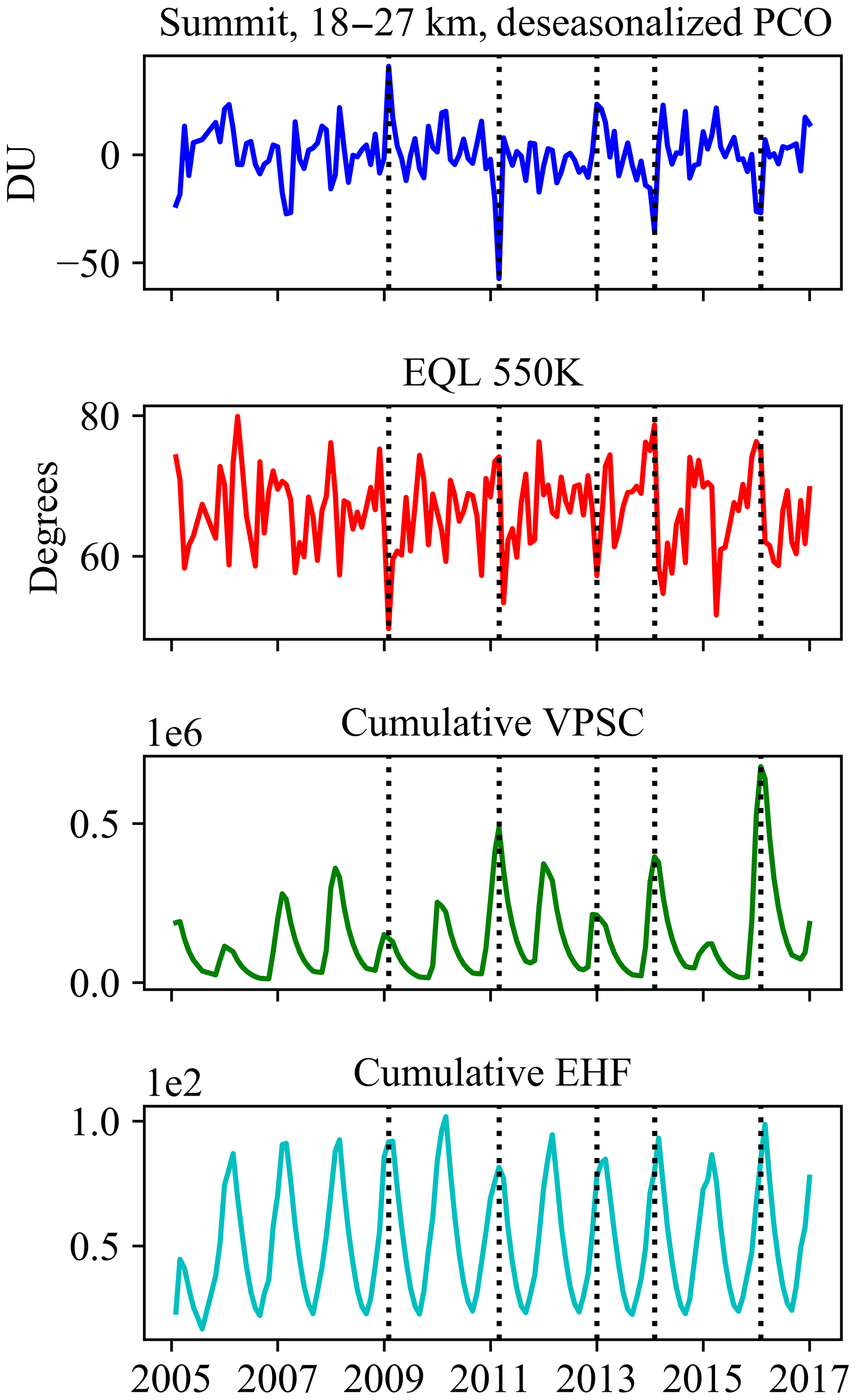
Figure 8Coincidence of extreme events in deseasonalized ozone over Summit Station (18–27 km; middle stratosphere) with the important proxies from Table 4. The vertical black dashed line shows the time of the extreme values of the deseasonalized ozone.
From the results in Table 2, we conclude that we have identified the important physical drivers of ozone variations at these four Arctic sites and within this sector of the Arctic. As an example of this analysis, Fig. 8 shows the time series of deseasonalized ozone and the selected proxies in middle stratosphere over Summit Station. The vertical dashed lines show the extreme values of ozone variations and how they coincide with extreme values in the different proxies. This provides confidence that our approach and the development of final models identify important physical processes that affect the ozone variations at these sites. Table 4 shows that TP, EHF, EQL, VPSC, and the QBO are all important drivers of ozone variations at these sites and that all of these proxies are necessary for a complete understanding of the variations in total column ozone.
There is continuing debate on what controls Arctic ozone and on the relative contributions of dynamics and photochemistry (Antsey and Shepard, 2014). Understanding what causes variations in Arctic ozone is particularly difficult because there are few long-term records of the vertical profile of ozone in this region. We present 12 years of vertical profiles of ozone over Summit Station, Greenland; Ny-Ålesund, Svalbard, Norway; and Alert and Eureka, Nunavut, Canada, from February 2005 to February 2017. Ozone profiles are created by merging ozonesonde profiles with ozone retrievals from the Microwave Limb Sounder, creating profiles from the surface to 60 km. The merged profile is of high quality because in situ measurements of ozone are used in the lower atmosphere, which accounts for an overestimation of ozone in this region by MLS. On the other hand, the MLS ozone profiles are quite accurate (2 %–3 %) in the stratosphere (above the maximum altitude reached by the ozonesondes; Livesey et al., 2017).
The analysis of the seasonal cycles at the different sites shows that they are, in general, similar but that significant differences exist from site to site. The TCO exhibits maxima in spring and minima in fall at all the sites. The PCO in the upper stratosphere peaks in summer at all the sites, with slightly larger values at Summit for most months. In the middle stratosphere, the seasonal cycle at Ny-Ålesund is shifted later by about 1 month, giving a delayed buildup of ozone in spring and decay in summer. The lower stratosphere shows the most significant differences in the seasonal cycle at the four sites, with Summit Station exhibiting an earlier decay in ozone from March to July and Ny-Ålesund showing a delay in ozone decay in summer. The seasonal cycle of tropospheric ozone variations peaks around May for Alert, Eureka, and Ny-Ålesund and in March at Summit; Summit also has significantly less ozone in the troposphere due to its high elevation. There are no significant trends in the multi-year annual TCO values at any of the sites. The most significant seasonal trends are seen at Ny-Ålesund, with positive trends in the summer and negative trends in the spring and fall; negative trends are also seen at Summit in summer and fall. However, we acknowledge the large uncertainty associated with these trends due to the short period of study. The seasonal cycles at each site explain the majority of ozone fluctuations in the TCO and the PCO in most of the atmospheric layers. However, the seasonal model explained fewer variations in the middle stratosphere than other atmospheric layers, except over Eureka.
We use a two-step approach to first determine the important drivers of ozone variations at the four high-latitude Arctic sites, and then we use these to develop models that explain the ozone variations. Stepwise multiple regression analysis is performed to determine significant proxies that affect ozone variations over the four sites. If a proxy is chosen at three or more of the four sites, then it is considered to be an important contributor in this sector of the Arctic. A final regression model is then fit to each time series. The final model is successful in identifying proxies that explain a significant portion of the ozone variance in the deseasonalized time series, with 90 % of the models with R2≥70 % and 40 % with R2≥80 %. The tropopause pressure, equivalent latitude at 370 K, and the QBO are important drivers between the surface and 10 km. The QBO, eddy heat flux, and the volume of polar stratospheric clouds are important in the lower stratosphere, while the equivalent latitude at 550 K, eddy heat flux, and the volume of polar stratospheric clouds strongly influence the middle and upper stratospheric ozone. The final regression model explains over 80 % of the variance in the time series of total column ozone at the four sites. The contribution from the important drivers is greatest at Summit Station, Greenland, in the troposphere (21 %) and middle stratosphere (32 %). In general, the important drivers explain the greatest variance at all the sites in the middle stratosphere, which is the region of the atmosphere that has the least variance explained by the seasonal cycle. Interestingly, the Arctic oscillation, solar flux. and El Niño–Southern Oscillation are not important for ozone variations in this sector of the Arctic.
Ozonesonde data for Summit Station, Greenland can be found at https://www.esrl.noaa.gov/gmd/dv/data/index.php?parameter_name=Ozone&site=SUM&type=Insitu (last access: 22 July 2019). Ozonesonde data for Alert, Eureka, and Ny-Ålesund can be found at https://woudc.org/data/explore.php?dataset=ozonesonde (last access: 22 July 2019). Data for the Microwave Limb Sounder (MLS) (Livesey and Read, 2015) can be found at https://acdisc.gesdisc.eosdis.nasa.gov/data/Aura_MLS_Level2/ML2O3.004/ (last access: 22 July 2019).
The supplement related to this article is available online at: https://doi.org/10.5194/acp-19-9733-2019-supplement.
SBS performed the data processing and analysis and drafted and edited the paper. VPW conceived the project, provided advice on the data analysis, and aided in drafting and editing the paper. IP, SO, BJ, PC, and CWS provided ozonesonde profiles from Summit. IP also edited the paper. DT provided ozonesonde data from Alert and Eureka and edited the paper. RK calculated the eddy heat flux dataset and edited the paper. LT calculated the dataset for the volume of polar stratospheric clouds. QE calculated the equivalent latitude dataset. All of the authors except SO discussed the scientific findings and contributed to the paper.
The authors declare that they have no conflict of interest.
We acknowledge useful discussions with Corinne Vigouroux from the Belgian Institute for Space Aeronomy, which helped formulate the analysis for this study. We thank Detlev Helmig (University of Colorado – Institute of Arctic and Alpine Research) for helpful discussions regarding the operation and response time of ECC ozonesondes. We are grateful to Timothy Ginn (Washington State University) for his useful suggestions regarding stepwise multiple regression modeling. We acknowledge the Ozone and Water Vapor Group at the Earth System Research Laboratory of the National Oceanic and Atmospheric Administration for use of the ozonesonde data and the science technicians at Summit Station, Greenland, for launching the ozonesondes. We acknowledge the World Ozone and Ultraviolet Radiation Data Centre (WOUDC) for providing Canadian and Norwegian ozonesondes. We acknowledge the National Aeronautics and Space Administration for the use of Microwave Limb Sounder data.
This research has been supported by the National Science Foundation, Division of Polar Programs (grant nos. PLR-1420932 and PLR-1414314).
This paper was edited by Andreas Engel and reviewed by two anonymous referees.
Allen, D. R. and Nakamura, N.: Tracer Equivalent Latitude: A Diagnostic Tool for Isentropic Transport Studies. J. Atmos. Sci., 60, 287–304, https://doi.org/10.1175/1520-0469(2003)060<0287:teladt>2.0.co;2, 2003.
Ancellet, G., Daskalakis, N., Raut, J. C., Tarasick, D., Hair, J., Quennehen, B., Ravetta, F., Schlager, H., Weinheimer, A. J., Thompson, A. M., Johnson, B., Thomas, J. L., and Law, K. S.: Analysis of the latitudinal variability of tropospheric ozone in the Arctic using the large number of aircraft and ozonesonde observations in early summer 2008, Atmos. Chem. Phys., 16, 13341–13358, https://doi.org/10.5194/acp-16-13341-2016, 2016.
Anstey, J. A. and Shepherd, T. G.: High-latitude influence of the quasi-biennial oscillation, Q. J. Roy. Meteorol. Soc., 140, 1–21, https://doi.org/10.1002/qj.2132, 2014.
Appenzeller, C., Weiss, A. K., and Staehelin, J.: North Atlantic Oscillation modulates total ozone winter trends, Geophys. Res. Lett., 27, 1131–1134, https://doi.org/10.1029/1999GL010854, 2000.
Ball, W. T., Alsing, J., Mortlock, D. J., Staehelin, J., Haigh, J. D., Peter, T., Tummon, F., Stübi, R., Stenke, A., Anderson, J., Bourassa, A., Davis, S. M., Degenstein, D., Frith, S., Froidevaux, L., Roth, C., Sofieva, V., Wang, R., Wild, J., Yu, P., Ziemke, J. R., and Rozanov, E. V.: Evidence for a continuous decline in lower stratospheric ozone offsetting ozone layer recovery, Atmos. Chem. Phys., 18, 1379–1394, https://doi.org/10.5194/acp-18-1379-2018, 2018.
Bowman, K. P.: Global Patterns of the Quasi-biennial Oscillation in Total Ozone, J. Atmos. Sci., 46, 3328–3343, https://doi.org/10.1175/1520-0469(1989)046<3328:gpotqb>2.0.co;2, 1989.
Brunner, D., Staehelin, J., Maeder, J. A., Wohltmann, I., and Bodeker, G. E.: Variability and trends in total and vertically resolved stratospheric ozone based on the CATO ozone data set, Atmos. Chem. Phys., 6, 4985–5008, https://doi.org/10.5194/acp-6-4985-2006, 2006.
Butchart, N. and Remsberg, E. E.: The Area of the Stratospheric Polar Vortex as a Diagnostic for Tracer Transport on an Isentropic Surface, J. Atmos. Sci., 43, 1319–1339, https://doi.org/10.1175/1520-0469(1986)043<1319:taotsp>2.0.co;2, 1986.
Christiansen, B., Jepsen, N., Kivi, R., Hansen, G., Larsen, N., and Korsholm, U. S.: Trends and annual cycles in soundings of Arctic tropospheric ozone, Atmos. Chem. Phys., 17, 9347–9364, https://doi.org/10.5194/acp-17-9347-2017, 2017.
Crutzen, P. J.: Ozone production rates in an oxygen-hydrogen-nitrogen oxide atmosphere, J. Geophys. Res., 76, 7311–7327, https://doi.org/10.1029/JC076i030p07311, 1971.
Damski, J., Thölix, L., Backman, L., Taalas, P., and Kulmala, M.: FinROSE – middle atmospheric chemistry and transport model, Boreal Environ. Res., 12, 535–550, 2007.
Danielsen, E. F.: Stratospheric-Tropospheric Exchange Based on Radioactivity, Ozone and Potential Vorticity, J. Atmos. Sci., 25, 502–518, https://doi.org/10.1175/1520-0469(1968)025<0502:stebor>2.0.co;2, 1968.
Deshler, T., Mercer, J., Smit, H., Stubi, R., Levrat, G., Johnson, B., Oltmans, S., Kivi, R., Thompson, A., Witte, J., Davies, J., Schmidlin, F., Brothers, G., and Sasaki, T.: Atmospheric comparison of electrochemical cell ozonesondes from different manufacturers, and with different cathode solution strengths: The Balloon Experiment on Standards for Ozonesondes, J. Geophys. Res., 113, D04307, https://doi.org/10.1029/2007JD008975, 2008.
Deshler, T., Stübi, R., Schmidlin, F. J., Mercer, J. L., Smit, H. G. J., Johnson, B. J., Kivi, R., and Nardi, B.: Methods to homogenize electrochemical concentration cell (ECC) ozonesonde measurements across changes in sensing solution concentration or ozonesonde manufacturer, Atmos. Meas. Tech., 10, 2021–2043, https://doi.org/10.5194/amt-10-2021-2017, 2017.
Doherty, R. M., Stevenson, D. S., Johnson, C. E., Collins, W. J., and Sanderson, M. G.: Tropospheric ozone and El Niño–Southern Oscillation: Influence of atmospheric dynamics, biomass burning emissions, and future climate change, J. Geophys. Res., 111, 3867, https://doi.org/10.1029/2005JD006849, 2006.
Ebdon, R. A.: The quasi-biennial oscillation and its association with tropospheric circulation pattern, Meteorol. Mag., 104, 282–297, 1975.
Eichelberger, S. J.: Changes in the strength of the Brewer-Dobson circulation in a simple AGCM, Geophys. Res. Lett., 32, 1990–1995, https://doi.org/10.1029/2005GL022924, 2005.
Forster, P. M. and Shine, K. P.: Radiative forcing and temperature trends from stratospheric ozone changes, J. Geophys. Res., 102, 10841–10855, https://doi.org/10.1029/96JD03510, 1997.
Fusco, A. C. and Salby, M. L.: Interannual Variations of Total Ozone and Their Relationship to Variations of Planetary Wave Activity, J. Climate, 12, 1619–1629, https://doi.org/10.1175/1520-0442(1999)012<1619:ivotoa>2.0.co;2, 1999.
Garfinkel, C. I. and Hartmann, D. L.: Effects of the El Niño–Southern Oscillation and the Quasi-Biennial Oscillation on polar temperatures in the stratosphere, J. Geophys. Res., 112, 3343–3413, https://doi.org/10.1029/2007JD008481, 2007.
Garfinkel, C. I. and Hartmann, D. L.: Different ENSO teleconnections and their effects on the stratospheric polar vortex, J. Geophys. Res., 113, D18114, https://doi.org/10.1029/2008JD009920, 2008.
Gaudel, A., Ancellet, G., and Godin-Beekmann, S.: Analysis of 20 years of tropospheric ozone vertical profiles by lidar and ECC at Observatoire de Haute Provence (OHP) at 44∘ N, 6.7∘ E, Atmos. Environ., 113, 78–89, https://doi.org/10.1016/j.atmosenv.2015.04.028, 2015.
Harris, N. R. P., Lehmann, R., Rex, M., and von der Gathen, P.: A closer look at Arctic ozone loss and polar stratospheric clouds, Atmos. Chem. Phys., 10, 8499–8510, https://doi.org/10.5194/acp-10-8499-2010, 2010.
Hasebe, F.: A Global Analysis of the Fluctuation of Total Ozone, J. Meteor. Soc. Japan. Ser. II, 58, 104–117, https://doi.org/10.2151/jmsj1965.58.2_104, 1980.
Holton, J. R. and Lindzen, R. S.: An Updated Theory for the Quasi-Biennial Cycle of the Tropical Stratosphere, J. Atmos. Sci., 29, 1076–1080, https://doi.org/10.1175/1520-0469(1972)029<1076:autftq>2.0.co;2, 1972.
Holton, J. R. and Tan, H.-C.: The Influence of the Equatorial Quasi-Biennial Oscillation on the Global Circulation at 50 mb, J. Atmos. Sci., 37, 2200–2208, https://doi.org/10.1175/1520-0469(1980)037<2200:tioteq>2.0.co;2, 1980.
Holton, J. R. and Tan, H.-C.: The Quasi-Biennial Oscillation in the Northern Hemisphere Lower Stratosphere, J. Meteor. Soc. Japan. Ser. II, 60, 140–148, https://doi.org/10.2151/jmsj1965.60.1_140, 1982.
Holton, J. R., Haynes, P. H., McIntyre, M. E., Douglass, A. R., Rood, R. B., and Pfister, L.: Stratosphere-troposphere exchange, Rev. Geophys., 33, 403–439, https://doi.org/10.1029/95RG02097, 1995.
Johnson, B. J., Oltmans, S. J., Vömel, H., Smit, H. G. J., Deshler, T., and Kröger, C.: Electrochemical concentration cell (ECC) ozonesonde pump efficiency measurements and tests on the sensitivity to ozone of buffered and unbuffered ECC sensor cathode solutions, J. Geophys. Res., 107, 7881, https://doi.org/10.1029/2001JD000557, 2002.
Kerr, J. B., Fast, H., McElroy, C. T., Oltmans, S. J., Lathrop, J. A., Kyro, E., Paukkunen, A., Claude, H., Köhler, U., Sreedharan, C. R., Takao, T., and Tsukagoshi, Y.: The 1991 WMO international ozonesonde intercomparison at Vanscoy, Canada, Atmos.-Ocean, 32, 685–716, 1994.
Kivi, R., Kyrö, E., Turunen, T., Harris, N. R. P., von der Gathen, P., Rex, M., Andersen, S. B., and Wohltmann, I.: Ozonesonde observations in the Arctic during 1989–2003: Ozone variability and trends in the lower stratosphere and free troposphere, J. Geophys. Res., 112, 2013–2017, https://doi.org/10.1029/2006JD007271, 2007.
Komhyr, W. D.: Electrochemical concentration cells for gas analysis, Ann. Geoph., 25, 203–210, 1969.
Komhyr, W. D.: Operations handbook-ozone measurements to 40-km altitude with model 4A electrochemical concentration cell (ECC) ozonesondes (used with 1680-MHz radiosondes), in Technical memorandum ERL ARL-149, NOAA, Boulder, Colorado, 49 pp., 1986.
Komhyr, W. D., Grass, R. D., and Leonard, R. K.: Dobson spectrophotometer 83: A standard for total ozone measurements, 1962–1987, J. Geophys. Res., 94, 9847–9861, https://doi.org/10.1029/JD094iD07p09847, 1989.
Kuttippurath, J., Godin-Beekmann, S., Lefèvre, F., Nikulin, G., Santee, M. L., and Froidevaux, L.: Record-breaking ozone loss in the Arctic winter 2010/2011: comparison with 1996/1997, Atmos. Chem. Phys., 12, 7073–7085, https://doi.org/10.5194/acp-12-7073-2012, 2012.
Li, K. F. and Tung, K. K.: Quasi-biennial oscillation and solar cycle influences on winter Arctic total ozone, J. Geophys. Res., 119, 5823–5835, https://doi.org/10.1002/2013JD021065, 2014.
Lindzen, R. S. and Holton, J. R.: A Theory of the Quasi-Biennial Oscillation, J. Atmos. Sci., 25, 1095–1107, https://doi.org/10.1175/1520-0469(1968)025<1095:atotqb>2.0.co;2, 1968.
Livesey, N. and Read, W.: MLS/Aura Level 2 Diagnostics, Geophysical Parameter Grid V004, Greenbelt, MD, USA, Goddard Earth Sciences Data and Information Services Center (GES DISC), https://doi.org/10.5067/Aura/MLS/DATA2006, 2015.
Livesey, N. J., Santee, M. L., and Manney, G. L.: A Match-based approach to the estimation of polar stratospheric ozone loss using Aura Microwave Limb Sounder observations, Atmos. Chem. Phys., 15, 9945–9963, https://doi.org/10.5194/acp-15-9945-2015, 2015.
Livesey, N. J., Read, W. G., Wagner, P. A., Froidevaux, L., Lambert, A., Manney, G. L., Millán Valle, L. F., Pumphrey, H. C., Santee, M. L., Schwartz, M. J., Wang, S., Fuller, R. A., Jarnot, R. F., Knosp, B. W., Martinez, E., and Lay, R. R.: Earth Observing System (EOS) Aura Microwave Limb Sounder (MLS) Version 4.2x× level 2 data quality and description document, 1–169, 2018.
Logan, J. A.: Trends in the vertical distribution of ozone: An analysis of ozonesonde data, J. Geophys. Res., 99, 25553–25585, https://doi.org/10.1029/94JD02333, 1994.
Logan, J. A., Megretskaia, I. A., Miller, A. J., Tiao, G. C., Choi, D., Zhang, L., Stolarski, R. S., Labow, G. J., Hollandsworth, S. M., Bodeker, G. E., Claude, H., de Muer, D., Kerr, J. B., Tarasick, D. W., Oltmans, S. J., Johnson, B., Schmidlin, F., Staehelin, J., Viatte, P., and Uchino, O.: Trends in the vertical distribution of ozone: A comparison of two analyses of ozonesonde data, J. Geophys. Res., 104, 26373–26399, https://doi.org/10.1029/1999JD900300, 1999.
Mäder, J. A., Staehelin, J., Brunner, D., Stahel, W. A., Wohltmann, I., and Peter, T.: Statistical modeling of total ozone: Selection of appropriate explanatory variables. J. Geophys. Res., 112, D11108, https://doi.org/10.1029/2006JD007694, 2007.
Manney, G. L., Santee, M. L., Rex, M., Livesey, N. J., Pitts, M. C., Veefkind, P., Nash, E. R., Wohltmann, I., Lehmann, R., Froidevaux, L., Poole, L. R., Schoeberl, M. R., Haffner, D. P., Davies, J., Dorokhov, V., Gernandt, H., Johnson, B., Kivi, R., Kyrö, E., Larsen, N., Levelt, P. F., Makshtas, A., McElroy, C. T., Nakajima, H., Parrondo, M. C., Tarasick, D. W., von der Gathen, P., Walker, K. A., and Zinoviev, N. S.: Unprecedented Arctic ozone loss in 2011, Nature, 478, 469–475, https://doi.org/10.1038/nature10556, 2011.
McDonald, M. K., Turnbull, D. N., and Donovan, D. P.: Steller Brewer, ozonesonde, and DIAL measurements of Arctic O3 column over Eureka, N.W.T. during 1996 winter/spring, Geophys. Res. Lett., 26, 2383–2386, https://doi.org/10.1029/1999GL900506, 1999.
Miller, A. J., Cai, A., Tiao, G., Wuebbles, D. J., Flynn, L. E., Yang, S.-K., Weatherhead, E. C., Fioletov, V., Petropavlovskikh, I., Meng, X.-L., Guillas, S., Nagatani, R. M., and Reinsel, G. C.: Examination of ozonesonde data for trends and trend changes incorporating solar and Arctic oscillation signals, J. Geophys. Res., 111, D13305, https://doi.org/10.1029/2005JD006684, 2006.
Nair, P. J., Godin-Beekmann, S., Kuttippurath, J., Ancellet, G., Goutail, F., Pazmiño, A., Froidevaux, L., Zawodny, J. M., Evans, R. D., Wang, H. J., Anderson, J., and Pastel, M.: Ozone trends derived from the total column and vertical profiles at a northern mid-latitude station, Atmos. Chem. Phys., 13, 10373–10384, https://doi.org/10.5194/acp-13-10373-2013, 2013.
Newchurch, M. J.: Evidence for slowdown in stratospheric ozone loss: First stage of ozone recovery, J. Geophys. Res., 108, 23079–23113, https://doi.org/10.1029/2003JD003471, 2003.
Randel, W. J., Garcia, R. R., Calvo, N., and Marsh, D.: ENSO influence on zonal mean temperature and ozone in the tropical lower stratosphere, Geophys. Res. Lett., 36, L15822, https://doi.org/10.1029/2009GL039343, 2009.
Rao, T. N.: Climatology of UTLS ozone and the ratio of ozone and potential vorticity over northern Europe, J. Geophys. Res., 108, 3451–3510, https://doi.org/10.1029/2003JD003860, 2003.
Rao, T. N., Arvelius, J., Kirkwood, S., and von der Gathen, P.: Climatology of ozone in the troposphere and lower stratosphere over the European Arctic, Adv. Space Res., 34, 754–758, https://doi.org/10.1016/j.asr.2003.05.055, 2004.
Rex, M., Salawitch, R. J., von der Gathen, P., Harris, N. R. P., Chipperfield, M. P., and Naujokat, B.: Arctic ozone loss and climate change, Geophys. Res. Lett., 31, L04116, https://doi.org/10.1029/2003GL018844, 2004.
Shepherd, T. G.: Dynamics, stratospheric ozone, and climate change, Atmos.-Ocean, 46, 117–138, https://doi.org/10.3137/ao.460106, 2008.
Smit, H. G. J. and Kley, D.: JOSIE.: The 1996 WMO International intercomparison of ozonesondes under quasi flight conditions in the environmental simulation chamber at Jülich, WMO Global Atmosphere Watch report series, No. 130 (Technical Document No. 926), World Meteorological Organization, Geneva, 1998.
Smit, H. G. J., Straeter, W., Johnson, B. J., Oltmans, S. J., Davies, J., Tarasick, D. W., Hoegger, B., Stubi, R., Schmidlin, F. J., Northam, T., Thompson, A. M., Witte, J. C., Boyd, I., and Posny, F.: Assessment of the performance of ECC-ozonesondes under quasi-flight conditions in the environmental simulation chamber: Insights from the Juelich Ozone Sonde Intercomparison Experiment (JOSIE), J. Geophys. Res., 112, 563–618, https://doi.org/10.1029/2006JD007308, 2007.
Solomon, S., Portmann, R. W., Sasaki, T., Hofmann, D. J., and Thompson, D. W. J.: Four decades of ozonesonde measurements over Antarctica, J. Geophys. Res., 110, 25877–25915, https://doi.org/10.1029/2005JD005917, 2005.
Staehelin, J., Harris, N. R. P., Appenzeller, C., and Eberhard, J.: Ozone trends: A review, Rev. Geophys., 39, 231–290, https://doi.org/10.1029/1999RG000059, 2001.
Steinbrecht, W., Claude, H., KöHler, U., and Hoinka, K. P.: Correlations between tropopause height and total ozone: Implications for long-term changes, J. Geophys. Res., 103, 19183–19192, https://doi.org/10.1029/98JD01929, 1998.
Steinbrecht, W., Froidevaux, L., Fuller, R., Wang, R., Anderson, J., Roth, C., Bourassa, A., Degenstein, D., Damadeo, R., Zawodny, J., Frith, S., McPeters, R., Bhartia, P., Wild, J., Long, C., Davis, S., Rosenlof, K., Sofieva, V., Walker, K., Rahpoe, N., Rozanov, A., Weber, M., Laeng, A., von Clarmann, T., Stiller, G., Kramarova, N., Godin-Beekmann, S., Leblanc, T., Querel, R., Swart, D., Boyd, I., Hocke, K., Kämpfer, N., Maillard Barras, E., Moreira, L., Nedoluha, G., Vigouroux, C., Blumenstock, T., Schneider, M., García, O., Jones, N., Mahieu, E., Smale, D., Kotkamp, M., Robinson, J., Petropavlovskikh, I., Harris, N., Hassler, B., Hubert, D., and Tummon, F.: An update on ozone profile trends for the period 2000 to 2016, Atmos. Chem. Phys., 17, 10675–10690, https://doi.org/10.5194/acp-17-10675-2017, 2017.
Sterling, C. W., Johnson, B. J., Oltmans, S. J., Smit, H. G. J., Jordan, A. F., Cullis, P. D., Hall, E. G., Thompson, A. M., and Witte, J. C.: Homogenizing and estimating the uncertainty in NOAA's long-term vertical ozone profile records measured with the electrochemical concentration cell ozonesonde, Atmos. Meas. Tech., 11, 3661–3687, https://doi.org/10.5194/amt-11-3661-2018, 2018.
Strahan, S. E. and Douglass, A. R.: Decline in Antarctic Ozone Depletion and Lower Stratospheric Chlorine Determined From Aura Microwave Limb Sounder Observations, Geophys. Res. Lett., 45, 382–390, https://doi.org/10.1002/2017GL074830, 2018.
Taguchi, M. and Hartmann, D. L.: Increased Occurrence of Stratospheric Sudden Warmings during El Niño as Simulated by WACCM, J. Climate, 19, 324–332, https://doi.org/10.1175/jcli3655.1, 2006.
Tarasick, D. W.: Changes in the vertical distribution of ozone over Canada from ozonesondes: 1980–2001, J. Geophys. Res., 110, 1131, https://doi.org/10.1029/2004JD004643, 2005.
Tarasick, D. W., Davies, J., Smit, H. G. J., and Oltmans, S. J.: A re-evaluated Canadian ozonesonde record: measurements of the vertical distribution of ozone over Canada from 1966 to 2013, Atmos. Meas. Tech., 9, 195–214, https://doi.org/10.5194/amt-9-195-2016, 2016.
Tarasick, D. W., Carey-Smith, T. K., Hocking, W. K., Moeini, O., He, H., Liu, J., Osman, M., Thompson, A. M., Johnson, B., Oltmans, S. J., and Merrill, J. T.: Quantifying stratosphere-troposphere transport of ozone using balloon-borne ozonesondes, radar windprofilers and trajectory models, Atmos. Environ., 198, 496–509, https://doi.org/10.1016/j.atmosenv.2018.10.040, 2019.
Thompson, D. W. J., Baldwin, M. P., and Wallace, J. M.: Stratospheric Connection to Northern Hemisphere Wintertime Weather: Implications for Prediction, J. Climate, 15, 1421–1428, https://doi.org/10.1175/1520-0442(2002)015<1421:SCTNHW>2.0.CO;2, 2002.
Vigouroux, C., De Mazière, M., Demoulin, P., Servais, C., Hase, F., Blumenstock, T., Kramer, I., Schneider, M., Mellqvist, J., Strandberg, A., Velazco, V., Notholt, J., Sussmann, R., Stremme, W., Rockmann, A., Gardiner, T., Coleman, M., and Woods, P.: Evaluation of tropospheric and stratospheric ozone trends over Western Europe from ground-based FTIR network observations, Atmos. Chem. Phys., 8, 6865–6886, https://doi.org/10.5194/acp-8-6865-2008, 2008.
Vigouroux, C., Blumenstock, T., Coffey, M., Errera, Q., García, O., Jones, N. B., Hannigan, J. W., Hase, F., Liley, B., Mahieu, E., Mellqvist, J., Notholt, J., Palm, M., Persson, G., Schneider, M., Servais, C., Smale, D., Thölix, L., and De Mazière, M.: Trends of ozone total columns and vertical distribution from FTIR observations at eight NDACC stations around the globe, Atmos. Chem. Phys., 15, 2915–2933, https://doi.org/10.5194/acp-15-2915-2015, 2015.
Walker T. W., Jones, D. B. A., Parrington, M., Henze, D. K., Murray, L. T., Bottenheim, J. W., Anlauf, K., Worden, J. R., Bowman, K. W., Shim, C., Singh, K., Kopacz, M., Tarasick, D. W., Davies, J., von der Gathen, P., Thompson, A. M. and Carouge, C. C.: Impacts of midlatitude precursor emissions and local photochemistry on ozone abundances in the Arctic, J. Geophys. Res., 117, D01305, https://doi.org/10.1029/2011JD016370, 2012.
Wallace, J. M.: General circulation of the tropical lower stratosphere, Rev. Geophys., 11, 191–222, https://doi.org/10.1029/RG011i002p00191, 1973.
Waters, J. W., Froidevaux, L., Harwood, R. S., Jarnot, R. F., Pickett, H. M., Read, W. G., Siegel, P. H., Cofield, R. E., Filipiak, M. J., Flower, D. A., Holden, J. R., Lau, G. K., Livesey, N. J., Manney, G. L., Pumphrey, H. C., Santee, M. L., Wu, D. L., Cuddy, D. T., Lay, R. R., Loo, M. S., Perun, V. S., Schwartz, M. J., Stek, P. C., Thurstans, R. P., Boyles, M. A., Chandra, K. M., Chavez, M. C., Gun-Shing Chen, Chudasama, B. V., Dodge, R., Fuller, R. A., Girard, M. A., Jiang, J. H., Yibo Jiang, Knosp, B. W., LaBelle, R. C., Lam, J. C., Lee, K. A., Miller, D., Oswald, J. E., Patel, N. C., Pukala, D. M., Quintero, O., Scaff, D. M., Van Snyder, W., Tope, M. C., Wagner, P. A. and Walch, M. J.: The Earth observing system microwave limb sounder (EOS MLS) on the aura Satellite, IEEE T. Geosci. Remote, 44, 1075–1092, https://doi.org/10.1109/TGRS.2006.873771, 2006.
Weatherhead, E. C. and Andersen, S. B.: The search for signs of recovery of the ozone layer, Nature, 441, 39–45, https://doi.org/10.1038/nature04746, 2006.
Weber, M., Coldewey-Egbers, M., Fioletov, V. E., Frith, S. M., Wild, J. D., Burrows, J. P., Long, C. S., and Loyola, D.: Total ozone trends from 1979 to 2016 derived from five merged observational datasets – the emergence into ozone recovery, Atmos. Chem. Phys., 18, 2097–2117, https://doi.org/10.5194/acp-18-2097-2018, 2018.
Wilks, D. S.: Statistical Methods in the Atmospheric sciences, 3 edn., Elsevier, Oxford, 676 pp., 2011.
WMO: Scientific assessment of ozone depletion: 2006, WMO Rep. 50, Global Ozone Research and Monitoring Project, 572, available at: http://www.wmo.int/pages/prog/arep/gaw/ozone_2006/ozone_asst_report.html (last access: 22 July 2019), 2007.
WMO: Assessment for Decision-Makers Scientiic Assessment of Ozone Depletion: 2014, WMO Rep. 55, 413, available at: http://www.wmo.int/pages/prog/arep/gaw/ozone_2014/documents/Full_report_2014_Ozone_Assessment.pdf (last access: 22 July 2019), 2014.
Wohltmann, I., Rex, M., Brunner, D., and Mäder, J.: Integrated equivalent latitude as a proxy for dynamical changes in ozone column, Geophys. Res. Lett., 32, L09811, https://doi.org/10.1029/2005GL022497, 2005.
Wohltmann, I., Lehmann, R., Rex, M., Brunner, D., and Mäder, J. A. A.: process-oriented regression model for column ozone, J. Geophys. Res.-Atmos., 112, 811–918, https://doi.org/10.1029/2006JD007573, 2007.
Wohltmann, I., Wegner, T., Müller, R., Lehmann, R., Rex, M., Manney, G. L., Santee, M. L., Bernath, P., Sumińska-Ebersoldt, O., Stroh, F., von Hobe, M., Volk, C. M., Hösen, E., Ravegnani, F., Ulanovsky, A., and Yushkov, V.: Uncertainties in modelling heterogeneous chemistry and Arctic ozone depletion in the winter 2009/2010, Atmos. Chem. Phys., 13, 3909–3929, https://doi.org/10.5194/acp-13-3909-2013, 2013.
Yang, E.-S., Cunnold, D. M., Salawitch, R. J., McCormick, M. P., Russell, J., III, Zawodny, J. M., Oltmans, S., and Newchurch, M. J.: Attribution of recovery in lower-stratospheric ozone, J. Geophys. Res., 111, 8399, https://doi.org/10.1029/2005JD006371, 2006.
Yang, X., Pyle, J. A., Cox, R. A., Theys, N., and Van Roozendael, M.: Snow-sourced bromine and its implications for polar tropospheric ozone, Atmos. Chem. Phys., 10, 7763–7773, https://doi.org/10.5194/acp-10-7763-2010, 2010.