the Creative Commons Attribution 4.0 License.
the Creative Commons Attribution 4.0 License.
 | 24 Jul 2019
A study on harmonizing total ozone assimilation with multiple sensors
Yves J. Rochon
Michael Sitwell
Young-Min Cho
Bias estimations and corrections of total column measurements are applied and evaluated with ozone data from satellite instruments providing near-real-time products during summer 2014 and 2015 and winter 2015. The developed standalone bias-correction system can be applied in near-real-time chemical data assimilation and long-term reanalysis. The instruments to which these bias corrections were applied include the Global Ozone Monitoring Experiment-2 instruments on the MetOp-A and MetOp-B satellites (GOME-2A and GOME-2B), the total column ozone mapping instrument of the Ozone Mapping Profiler Suite (OMPS-NM) on the Suomi National Polar-orbiting Partnership (S-NPP) satellite, and the Ozone Monitoring Instrument (OMI) instrument on the Aura research satellite. The OMI data set based on the TOMS version 8.5 retrieval algorithm was chosen as the reference used in the bias correction of the other satellite-based total column ozone data sets. OMI data were chosen for this purpose instead of ground-based observations due to OMI's significantly better spatial and temporal coverage, as well as interest in near-real-time assimilation. Ground-based Brewer and Dobson spectrophotometers, and filter ozonometers, as well as the Solar Backscatter Ultraviolet satellite instrument (SBUV/2), served as independent validation sources of total column ozone data. Regional and global mean differences of the OMI-TOMS data with measurements from the three ground-based instrument types for the three evaluated 2-month periods were found to be within 1 %, except for the polar regions, where the largest differences from the comparatively small data set in Antarctica exceeded 3 %. Values from SBUV/2 summed partial columns were typically larger than OMI-TOMS on average by 0.6 % to 1.2 %, with smaller differences than with ground-based observations over Antarctica. Bias corrections as a function of latitude and solar zenith angle were performed for GOME-2A/B and OMPS-NM using colocation with OMI-TOMS and three variants of differences with short-term model forecasts. These approaches were shown to yield residual biases of less than 1 %, with the rare exceptions associated with bins with less data. These results were compared to a time-independent bias-correction estimation that used colocations as a function of ozone effective temperature and solar zenith angle which, for the time period examined, resulted in larger residual biases for bins whose bias varies more in time.
The impact of assimilating total column ozone data from single and multiple satellite data sources with and without bias correction was examined with a version of the Environment and Climate Change Canada variational assimilation and forecasting system. Assimilation experiments for July–August 2014 show a reduction of global mean biases for short-term forecasts relative to ground-based Brewer and Dobson observations from a maximum of about 2.3 % in the absence of bias correction to less than 0.3 % in size when bias correction is included. Both temporally averaged and time-varying mean differences of forecasts with OMI-TOMS were reduced to within 1 % for nearly all cases when bias-corrected observations are assimilated for the latitudes where satellite data are present.
- Article
(3181 KB) - Full-text XML
-
Supplement
(877 KB) - BibTeX
- EndNote


The works published in this journal are distributed under the Creative Commons Attribution 4.0 License. This license does not affect the Crown copyright work, which is re-usable under the Open Government Licence (OGL). The Creative Commons Attribution 4.0 License and the OGL are interoperable and do not conflict with, reduce or limit each other.
© Crown copyright 2019
Total column ozone biases from satellite measurements are typically within a few percent. Changes of a few percent over time or between instruments are significant in affecting the correct identification of long-term trends. Near-global reductions in column ozone were −1.8 % per decade from 1980 to the mid-1990s, while increases over the past 2 decades are at only 0.4 % to 0.6 % per decade (Steinbrecht et al., 2018). A requirement on the long-term stability of corrected total column ozone observations of 1 %–3 % per decade was specified by the Ozone-cci project of the European Space Agencies' Climate Change Initiative programme in Table 5 of van Weele (2016). This table also indicates accuracy requirements on total column ozone measurements of 2 % for facilitating research on the evolution of the ozone layer from radiative forcing and 3 % for studies on short-term, seasonal, and interannual variability. As an example, for an accuracy requirement of 2 % and measurement precisions between 1.0 % and 1.7 %, biases need to be no larger than about 1.7 % to 1.0 %, respectively. The comparison of column ozone data from different instruments allows for the identification of the level of agreement between data sets, potentially under various conditions, and can highlight cases and conditions with small to large relative biases. As such, sources that provide accurate and stable long-term data sets can potentially be used to provide corrections for other sources.
The validation of satellite remote sounding products usually includes a comparison to ground-based measurements, which provide a long-term reference record. For satellite instruments measuring column ozone, this typically consists of comparisons to Brewer and Dobson spectrophotometers, and potentially filter ozonometers. The main advantage of ground-based versus satellite total column ozone measurements is that they can view the Sun directly as opposed to relying on the backscatter of solar radiation, reducing the complexity and error sources of the retrievals. The final resulting systematic errors of the calibrated ground-based total column ozone daily averages for well-calibrated and maintained Brewer and Dobson instruments are no larger than ∼1.5 %–2 %, excluding sites with outlier characteristics (considering Fioletov et al., 1999, 2008). Much of the ground-based total column ozone data may be available soon after the measurements, with the original calibration usually being sufficient. For exceptional cases where the original calibration may have been faulty, a final calibration for the ground-based total column ozone may lag by 1 to 2 years from near real time. Previous studies have examined the dependence of the differences between satellite-based and ground-based total column ozone measurements on latitude, solar zenith angle, viewing zenith angle (i.e., cross-track differences), seasonal dependence, cloud cover, reflectivity, and the ozone effective temperature, as well as other factors. These dependencies have been studied for instruments such as the Ozone Monitoring Instrument (OMI; Balis et al., 2007a; Viatte et al., 2011; Koukouli et al., 2012; Bai et al., 2016), the Global Ozone Monitoring Experiment-2 (GOME-2; Balis et al., 2007b; Antón et al., 2009a, 2011; Loyola et al., 2011; Koukouli et al., 2012, 2015; Lerot et al., 2014; Hao et al., 2014; Garane et al., 2018), and the Ozone Mapping Profiler Suite (OMPS; Bai et al., 2016; Flynn et al., 2014). This includes examining the long-term stability of differences as done by van der A et al. (2010, 2015). In this paper, an observation data set that serves as a reference in a bias estimation is referred to as the anchor. Reanalysis studies covering many years, such as van der A et al. (2010, 2015), have directly used ground-based data as the anchor. A limitation in the use of ground-based observations as an anchor in bias estimation is that these observations are only available for certain locations, leaving many areas uncovered, especially in the Southern Hemisphere and over oceans. For the Southern Hemisphere, the applied bias parameterization may not necessarily capture as much of the spatial or instrument-to-instrument variations of the bias as compared to using observations from a satellite-borne instrument that covers a larger domain. If a satellite-based anchor is employed, it should ideally be in good agreement with ground-based measurements. Considering the limited projected lifetimes and possible deteriorations or failures of satellite-based instruments, transitions to new references would also be required in an operational setting.
Total column ozone bias estimation for observations can be performed in different ways and depend on different factors, such as the solar zenith angle (SZA), latitude, and season. Seasonal and related latitudinal changes in biases may result from limitations in retrieval algorithms. For example, the retrieval algorithm might not adequately account for the temperature dependence of the ozone absorption coefficients. Differences and limitations in accounting for clouds and surface albedos may also contribute to errors in total column ozone (e.g., Antón et al., 2009b). Bias parameterizations may range from being spatially and temporally global to more local.
The harmonization of different data sets through bias correction can be applied for standalone analyses, for reanalyses, and in near-real-time data assimilation. The assimilation process consists of introducing information from observations into model forecasts through the generation of analyses, the statistical blend of earlier forecast and observations, which serve as the initial conditions for subsequent forecasts. The assimilation of column and stratospheric ozone measurements for ozone-layer forecasting has been conducted mostly as of about 25 years ago, ultimately culminating in operational ozone-layer and UV-index forecasts (e.g., Lahoz and Errera, 2010; Inness et al., 2013). This typically involves the utilization of measurements from single to multiple satellite remote sounding instruments with the use of ground-based and other remote sounding data for independent verifications and, occasionally, bias correction.
Traditionally, the assimilation process assumes that both the model forecasts and observations are statistically unbiased following an initial spin-up time (unless biases are estimated within the analysis step). Unremoved biases or systematic errors in the observations or forecasting model can potentially impact the quality of the analyses and forecasts (e.g., Dee, 2005; Dragani and Dee, 2008). This is important for total column ozone when it comes to monitoring for multi-decadal trends, as referenced in van der A et al. (2010), for both trends inferred from just the observations alone or from their use within a data assimilation system. Generally, while the effectiveness of bias-correction schemes in removing biases is constrained by limited knowledge of the truth, their impact in reducing relative biases between different assimilated observations and/or correlated fields can potentially be just as significant for improved forecasting. An example of the latter is in multivariate assimilation, where ozone and meteorological assimilation can be coupled (e.g., Dee, 2008; Dee et al., 2011).
Ideally, the anchor used within a bias-correction scheme should be accurate, have a wide range of coverage in both space and time, and for near-real-time applications be available within a few hours or less after measurements are taken. The summed partial columns from SBUV/2 satellite instruments have been recommended as an anchor for long-term studies (Labow et al., 2013). This is due to the long-term coverage provided by the series of SBUV/2 instruments, combined with the low variations in time of the differences between these instruments and ground-based data (usually within ±1 %, but reduced for recent years). Labow et al. (2013) also showed differences over time of SBUV/2 with OMI data having remained within about 1 % and 2 % for the Northern Hemisphere (based on the Total Ozone Mapping Spectrometer (TOMS) version 8.5 total column retrieval algorithm, an enhancement of the version 8 algorithm described by Bhartia and Wellemeyer, 2002). McPeters et al. (2015), showing similar magnitudes and stability of differences in time, concluded that OMI-TOMS data could be used in trend studies. The merging of OMI with SBUV/2 and earlier TOMS instrument data for this purpose was performed by Chehade et al. (2014).
The focus of this study is bias estimation and correction of column ozone for multiple satellite sensors, towards eventual use in near-real-time data assimilation. The bias-estimation and bias-correction methods developed in this study may be integrated into an assimilation scheme that could be applied in near real time and can be utilized for other constituents. In this paper, we evaluate several different bias-estimation schemes used to correct observations of column ozone from satellite-borne instruments. Most of these methods utilize colocated observation sets for bias estimation. From this consideration, OMI-TOMS was chosen as the anchor for bias estimation and correction, as its dense spatial coverage allows for more colocations with measurements from other instruments. As part of this work, the OMI-TOMS column ozone data were evaluated using ground-based Brewer, Dobson, and filter ozonometer observations, as well as compared to SBUV/2 column ozone, for the limited time periods in this study. For these data sets, a target maximum residual bias of 1 % following bias corrections was selected. This satisfies the column ozone 2 % accuracy requirement from the European Space Agencies' Climate Change Initiate programme (van Weele, 2016) for random error levels of up to 1.7 %.
In this paper, we examine several bias-correction methods that use a discrete binning in latitude and solar zenith angle that, unlike a functional parameterization, allows for arbitrary nonlinear dependencies. In addition, an alternative estimation method involving the dependency on the ozone effective temperature (the mean temperature weighted by the ozone profile), as employed in van der A et al. (2010, 2015), was explored. As discussed later in the paper, dependencies on factors such as changes in cloud cover and viewing zenith angle were not examined.
Following bias estimation, data assimilations of column ozone observations from individual and multiple satellite instruments were conducted with and without bias correction. The impacts on the resulting 6 h forecasts were then assessed. The assimilations were conducted with the Environment and Climate Change Canada (ECCC) meteorological assimilation system adapted for constituent assimilation. These assimilations were univariate ozone assimilations and utilized operational ECCC meteorological analyses. The data sources assimilated in this study and correspondingly involved in the bias-estimation analysis are the GOME-2 instruments on the European MetOp-A and MetOp-B satellites (Munro et al., 2016; Hassinen et al., 2016), the total column measuring instruments of OMPS (Dittman et al., 2002a, b; Flynn et al., 2006) on the Suomi National Polar-orbiting Partnership (S-NPP) satellite, and OMI aboard the Aura research satellite (Levelt et al., 2018).
This paper is organized as follows: Sect. 2 describes the utilized ozone observations covering July–August 2014 and 2015 and January–February 2015. Following a general quality assessment of the OMI data based on the available literature, Sect. 3 evaluates the OMI-TOMS column ozone data for these periods against ground-based measurements. Having assessed the quality of the OMI-TOMS data for these specific periods, Sect. 4 describes and applies three different bias-estimation approaches with the column ozone measurements of different satellite instruments relative to OMI. Following a description of the assimilation system, the impact of column ozone assimilation on 6 h forecasts for individual and multiple sensors with and without bias corrections is examined in Sect. 5 for July–August 2014 using comparisons to both OMI-TOMS and ground-based data. Conclusions are provided in Sect. 6. The Supplement for this paper provides additional figures and tables supporting and complementing the discussed and presented results.
In this section, we give a brief description of the column ozone observations involved in the implementation and evaluation of bias correction, in data assimilation, and in the validation of short-term forecasts. Observational data sets were obtained for the periods of July–August of 2014 and 2015, and January–February 2015. The main data sources of interest are those specifically intended to provide satellite-based column ozone allowing near-real-time (NRT) assimilation. These consist of OMI, GOME-2, and OMPS-NM (total column Nadir Mapper) instruments that rely on optical solar backscatter of ultraviolet radiation in the nadir or near-nadir and provide data only during daytime. Ground-based Brewer, Dobson, and ozonometer filter instruments and additional satellite-based data from OMPS-NP (partial column Nadir Profiler) and SBUV/2 are included for evaluation and validation purposes.
2.1 OMI
The Ozone Monitoring Instrument (OMI) aboard the Aura research satellite has been in operation since August 2004. The instrument stems from a collaboration between the Netherlands Agency for Aerospace Programmes (NIVR), now called the Netherlands Space Office (NSO), and the Finnish Meteorological Institute (FMI). The OMI instrument provides a cross-track width of about 2600 km on the ground and total column ozone mapping at a spatial resolution of 13 km along, and 24 km across, the orbit ground track at nadir (e.g., Bhartia and Wellemeyer, 2002; OMI Data User's Guide, 2012). Some strips of the OMI measurement tracks were removed due to the row anomaly of the OMI instrument, which for the time period under consideration affects 23 of the 60 rows (see http://projects.knmi.nl/omi/research/product/rowanomaly-background.php (last access: 15 July 2019) for more information and updates regarding the OMI row anomaly).
This study employs the OMS-TOMS V8.5 standard science column ozone data produced by NASA based on the Total Ozone Mapping Spectrometer (TOMS) total column retrieval algorithm. The OMI-TOMS algorithm (Bhartia and Wellemeyer, 2002) principally utilizes only two different wavelengths, one with strong and one with weak ozone absorption, to estimate the total column ozone and surface reflectivity. The OMI-TOMS column ozone has estimated root-mean-squared errors of 1 %–2 % (OMI Data User's Guide, 2012). The OMS-TOMS V8.5 standard science product is close to, but can differ slightly from, the OMI-TOMS NRT data (OMI NRT Data User's Guide, 2010; Durbin et al., 2010). The OMI NRT Data User's Guide (2010) and Durbin et al. (2010) indicate a daily maximum percentage difference of 2.6 % between the standard science and NRT products, with a weekly average maximum difference of 1.4 %. Further comparisons by the authors show mean differences generally between 0.02 % and 0.04% in July–August 2016 and January–February 2017. While not used here, the other common OMI total column ozone retrieval products are based on the Differential Optical Absorption Spectroscopy (DOAS) algorithm (Veefkind and de Haan, 2002; Veefkind et al., 2006; Kroon et al., 2008) from the Royal Netherlands Meteorological Institute (KNMI).
2.2 GOME-2
Global Ozone Monitoring Experiment-2 (GOME-2) instruments are on the MetOp-A (GOME-2A) and MetOp-B (GOME-2B) polar-orbiting satellites, launched in October 2006 and September 2012, respectively, and are operated by the European Organization for the Exploitation of Meteorological Satellites (EUMETSAT). As of 15 July 2013, GOME-2A has been operating with a swath width of 960 km and a 40 km × 40 km spatial resolution, while GOME-2B has a larger swath width of 1920 km and a 40 km × 80 km spatial resolution (e.g., GOME-2 ATBD, 2015; ATBD stands for the Algorithm Theoretical Basis Document).
The GOME-2 NRT products used here, as well as those for OMPS and SBUV/2, were acquired from the National Environmental Satellite, Data, and Information Service (NESDIS/NOAA) and stem from the TOMS approach. More specifically, the GOME-2 retrieved data products are from the TOMS V8 algorithm (Zhang and Kasheta, 2012). Alternatively, EUMETSAT provides GOME-2 total column ozone data based on the DOAS retrieval approach (Loyola et al., 2011; GOME User Manual, 2012; GOME-2 ATBD, 2015).
2.3 OMPS
The Ozone Mapping Profiler Suite (OMPS) on the Suomi National Polar-orbiting Partnership (S-NPP) satellite, launched in October 2011, consists of a combined nadir mapper (OMPS-NM) and nadir profiler (OMPS-NP) and a separate limb profiler (OMPS-LP), which provide total column, partial column profile, and limb profile products, respectively. A second suite was placed onboard the Joint Polar Satellite System JPSS-1 satellite (Zhou et al., 2016), renamed NOAA-20 and launched in November 2017. The retrieved data used in this study are from the OMPS S-NPP nadir measurements and are considered to be at a provisional product maturity level. They do not include improvements from the various corrections, calibration adjustments, and retrieval algorithm updates performed since the original near-real-time acquisition for the July–August 2014 period (Lawrence E. Flynn, NOAA, personal communication, 2016). The OMPS-NM and OMPS-NP ozone retrievals from the SBUV V8.6 retrieval algorithms (Bhartia et al., 2013; as referred to by Bai et al., 2016) became available after the completion of the assimilation experiments conducted for this work.
The OMPS-NM retrievals, summarized by Flynn et al. (2014), were made at the NOAA Interface Data Processing Segment using the ratio of the measured Earth radiances to solar irradiances at multiple triplets of wavelengths. The nadir mapper has a cross-track width of about 2800 km and a 50 km × 50 km resolution at nadir. Flynn et al. (2014) provide total column ozone accuracy and precision requirements of ∼3.5 %–4 % and ∼2 %, respectively, for SZA up to 80∘, and found average biases of −2 % to −4 % with respect to the OMI-TOMS and the Solar Backscatter Ultraviolet SBUV/2 satellite instrument products.
OMPS-NP profiles, each with a 250 km × 250 km field of view on the ground, were provided from an implementation of the Version 6 SBUV/2 instrument algorithm (Bhartia et al., 1996) with the a priori profiles derived from OMPS-NM. This version of the OMPS-NP data provides profiles of 12 layers. See Flynn et al. (2104) for a description of the accuracy and precision of the OMPS-NP V6 products. While only the nadir mapper data were assimilated in Sect. 5, both the nadir mapper and the summed partial columns of the nadir profiler were evaluated during bias correction.
2.4 Independent verification sources
Both ground-based and satellite-based column ozone data serve as independent verifications of the OMI-TOMS measurements, with the former also used for validation of the forecasts resulting from data assimilation. These data are described below.
2.4.1 Ground-based data
The ground-based data consist of Brewer, Dobson, and filter ozonometer total column ozone measurements (Fioletov et al., 1999, 2008; Staehelin et al., 2003) from the World Ozone and Ultraviolet Radiation Data Center (WOUDC) and of Brewer and Dobson measurements from the Global Monitoring Division of the NOAA Earth System Research Laboratory (see Coldewey-Egbers et al., 2015, for various references on the validation of column ozone satellite data with ground-based Brewers and Dobsons). Only direct-Sun, clear-sky daily daytime averages from these instruments were used. The error standard deviations for Brewer and Dobson direct-Sun data are no larger than ∼1.5 % to 2.0 % for well-calibrated and well-maintained instruments and about 1.5 to 2 times larger for filter ozonometers (Fioletov et al., 1999, and references therein; Fioletov et al., 2008). Consistent with the above, an overall precision of 4.6 DU has been obtained by van der A et al. (2010) for Brewer and Dobson direct-Sun daily averages, excluding outlier data. As in van der A et al. (2010) and Koukouli et al. (2016), the Dobson ozone values were adjusted following the correction of Komhyr et al. (1993; see also van Roozendael et al., 1998) as a function of ozone effective temperature (−0.13 % K−1 about 227 K). This correction is not applied to Brewer data in this study following van der A et al. (2010) based on the results presented in Kerr (2002).
2.4.2 SBUV/2
Data from the Solar Backscatter Ultraviolet instrument (SBUV/2) were used for verification purposes. The ozone data from SBUV/2 for the period of interest are from the NOAA 19 satellite (Flynn, 2007; Bhartia et al., 2013; McPeters et al., 2013). Two versions of the total column ozone data are used here. The first is from the SBUV V8.6 profile retrieval using wavelengths in the range of 250 to 310 nm (Bhartia et al., 2013; summarized by McPeters et al., 2013; see also Flynn, 2007) for which the total column ozone is the sum of the partial column layers, and the second is from the SBUV V8 total column retrieval using two wavelengths between 310 and 331 nm (Flynn, 2007; Flynn et al., 2009). The ozone measurements cover 170 km × 170 km field of views at the ground and have separations along the satellite orbit tracks of about 170 km. Labow et al. (2013) found the agreement between total column ozone data of SBUV instruments from the summed partial columns and the Northern Hemisphere ground-based data to be better than 1 %. Bhartia et al. (2013) have indicated that the total column ozone values resulting from the V8.6 algorithm can be used for solar zenith angles of up to 88∘.
Differences between OMI-TOMS and ground-based Brewer and Dobson data have shown long-term stability and relatively little solar zenith angle and latitude dependence (Balis et al., 2007a; Koukouli et al., 2012; Labow et al., 2013; McPeters et al., 2008, 2015). Comparisons of OMI-TOMS V8.5 total column ozone with Northern Hemisphere ground-based data by Labow et al. (2013) and McPeters et al. (2015) based on multiple years indicate an average underestimation of OMI-TOMS of about 1.5 %. Figure 2 of McPeters et al. (2015) shows variations of weekly mean differences about the long-term average underestimation mostly within about ±1 %. With OMI-TOMS V8, McPeters et al. (2008) found positive average differences with Northern Hemisphere Brewers and Dobsons covering 2005 and 2006 of 0.4 %, with a station-to-station standard deviation of 0.6 %. Also, OMI-TOMS total column ozone data show little to no dependency on cloud fraction, reflectivity, or cloud top pressure (< 1 %, but up to ∼2 % for cloud top pressure) (Balis et al., 2007b; Antón et al., 2009b; Antón and Loyola, 2011; Koukouli et al., 2012; Bak et al., 2015; Bai et al., 2015). van der A et al. (2010, 2015) indicate negligible variation with viewing zenith angle. For these reasons, and the near-global daily spatial coverage of its measurements, the OMI-TOMS total column ozone product was selected as the anchor in the bias-correction schemes described in Sect. 4.
To further examine the acceptability of using OMI-TOMS as a reference for bias correction, a mean differences comparison of OMI-TOMS V8.5 with near-colocated ground-based data at available sites over the periods of study was conducted. The colocation requirements are the same as those specified in Sect. 4.1 for the inter-comparison of satellite sensors. Summary results are shown in Table 1 and Fig. 1 (see also Tables S1 to S3). Bimonthly mean differences over regions, globally, and for the individual stations, were produced for the three periods of Table 1 based on totals of 53 Brewer, 40 Dobson, and 20 filter ozonometer stations. Figure 1 shows the station locations and mean differences for the July–August 2014 period. The sizes of the global mean differences over the different periods are in the approximate ranges of 0.0 % to −0.1 % for Brewer, −0.2 % to 0.4 % for Dobson, and −0.8 % to −0.7 % for filter ozonometer instruments. These global and regional averages exclude stations with mean differences larger than 2 standard deviations of the initial mean differences, corresponding to between 3 % and 4 %; this outlier removal process was also applied to each station in determining the mean differences at the stations. The total number of outlier stations per time period ranges from 0 to 5 (Tables S1 to S3), some of which are stations at high elevation or in Antarctica. While excluded from contributing to the global averages of Table 1, the outlier station mean differences in Antarctica were included as part of the regional mean differences for 60–90∘ S in Table 1, with a related discussion later in this section. The global mean differences, and most regional values, are typically smaller than earlier studies mentioned in the first paragraph. Possible contributors to this might be differences in time periods, region specifications, ground-based observation sets, or colocation conditions.
Table 1Regional and global relative mean differences (%) of total column ozone between OMI-TOMS and the specified ground-based instrument types over July–August 2014/2015 and January–February 2015. The averaging excludes stations having outlier station mean differences for each period (see Supplement tables S1 to S3 and the text of Sect. 3), except for the two rows for the latitude region 60–90∘ S as described in the text. The standard deviations (SDs) are for the inter-station variation of the mean differences about the regional or global mean differences. Unavailable SD values for available mean differences imply the presence of only one station. The Dobson total column ozone measurements for the two July–August periods were adjusted as a function of the ozone effective temperature (see Sect. 2.4); those for the January–February period were not adjusted in the absence of the ozone effective temperature for the period. The impacts of the Dobson July–August period corrections on the global mean differences were reductions between 0.0 % and 0.4 %.
a Outlier mean difference from the Marambio station. b includes the Amundsen–Scott, Marambio and outlier Zhongshan stations. c includes Marambio and Syowa stations. d Outlier Syowa station only. e Amundsen–Scott, Marambio and Syowa stations.

Figure 1Mean total column ozone differences (%) between OMI-TOMS and Brewer, Dobson, and filter ozonometer measurements over July–August 2014. The colours blue to purple denote negative differences and the colours yellow to red refer to positive differences.
The regional mean differences are within 1 %, with the exceptions being Antarctica for both the Brewer and Dobson instruments and the region of the North Pole for Dobson and filter ozonometer instruments. The mean differences for both polar regions are all negative, indicating an underestimation of OMI-TOMS column ozone in these regions for these periods relative to ground-based data, which is likely related to high SZAs. The mean differences for Dobsons and filters are similar to each other but slightly larger than for Brewers, despite error levels for the filter instruments being about 1.5 to 2 times larger (Sect. 2.4.1) and the small data sets.
More severe underestimations of OMI-TOMS relative to ground-based observations of 3 %–6 % occur during July–August in Antarctica, which is associated with SZAs close to or greater than 80∘ and possibly a strong latitudinal gradient associated with the winter South Pole polar vortex. While the small size of the data set of one to three stations in this region restricts the statistical significance of these results, the level of consistency between the instruments and sites suggests that it is worthwhile considering these data, and so they were retained in Table 1 for the rows of the 60–90∘ S region.
While not done here, a correction specifically for high SZAs could be envisaged, as done by van der A et al. (2015). While the OMI-TOMS data could be underestimating the total column ozone in the polar regions for these periods, there may be some uncertainty as to the actual OMI-TOMS bias. Factors that could affect the reliability of the comparison with the ground-based data at high solar zenith angles for Antarctica, beyond the low number of ground-based observations, include retrieval assumptions about the ozone layer (e.g., Bernhard et al., 2005), stray light sensitivity (especially for Dobsons; e.g., Moeini et al., 2019; Evans et al., 2009), and spatial gradients in the vicinity of the polar vortex.
Excluding the uncertainty in quantifying corrections in the region of the South Pole, the low mean differences of the OMI-TOMS V8.5 data with the ground-based data for most regions support not having to adjust the OMI-TOMS data before serving as an anchor in the bias estimation for the limited period covered in this study.
Observation biases can be examined as a function of various factors. In this study, the bias correction applied in the assimilation experiments used bias estimates for discrete SZA/latitude bins as a function of time. Different bias-estimation methods based on observation colocations and observation differences with forecasts will be examined. Solar zenith angle dependence is specifically included considering the varying sensitivities between the different instruments as shown in Koukouli et al. (2012). Latitude and time dependencies were introduced to capture other data processing biases as well as instrumental changes over time. The alternative method of using the dependence on the ozone effective temperature instead of latitude and time (e.g., van der A et al., 2010) was also explored. Any bias impact due to differences in spatial resolutions of the instruments or model forecasts would be part of the residual biases and associated representativeness errors. The effect of different resolutions between instruments in bias estimation would in part be mitigated by use of local averages of differences in space. While the dependency on other factors such as cloud cover and viewing zenith angle can vary with the instrument and retrieval algorithm, they are not included here as predictors. Their impact would then be reflected in the estimated standard deviations derived for observations. The bias-correction target is to reduce residual biases as a function of SZA and latitude relative to OMI-TOMS to within 1 %.
Both July–August and January–February periods are considered for a comparison of bias estimates between seasons within a yearly cycle. The two sets of SBUV/2 total column ozone values obtained from the two-wavelength retrieval (SBUV/2-TC) and the sum of the retrieved partial column profiles (SBUV/2-NP) are included in the comparisons to OMI-TOMS. These have been added to extend the evaluation of the OMI-TOMS data conducted in Sect. 3.
4.1 Colocation approach
This method estimates the bias as the mean differences of colocated observations with OMI-TOMS. Separate bias estimations are conducted for each distinct instrument platform. Here, the criteria for observations to be considered colocated are for the points to be within 200 km and ±12 h, and to have solar zenith angle differences smaller than 5∘ for SZA under 70∘ and smaller than 2∘ for SZA between 70 and 90∘. The latitude and solar zenith angle bins each have a size of 5∘ for the total column ozone products and 10∘ for summed partial column ozone profiles, except for solar zenith angles above 70∘, where bin sizes are reduced to 2∘. In any case, only data with SZA under 84∘ are used in assimilation considering the larger uncertainties at higher SZA. The smaller bins at high SZA were chosen since stronger gradients in the differences between instruments arise for these values. The larger bin sizes for summed partial column ozone profiles are in consideration of the smaller density of profile measurements. The resultant bias corrections are assigned to the midpoint of each bin and a two-dimensional piecewise linear interpolation is applied for intermediate SZA and latitude values; data that would require corrections from extrapolation are instead discarded.
Mean differences for each latitude/SZA bin are generated for individual 6 h intervals with, as a precaution, the removal of outliers beyond 2 standard deviations about the initial mean when there are at least 100 points per bin. Instead of monthly mean bias estimation, a moving window using the previous 2 weeks of data was applied to better capture variations in time. The 6 h mean differences over the 2-week moving window were weighted in time with a Gaussian weighting function with a half width at half maximum of 4.7 d. The 6 h mean differences were generated starting 2 weeks prior to the start of assimilations to provide data over the full window at the start of the assimilation. Another 2 standard deviation outlier removal was applied, this time according to the variability of the 6 h mean differences over the 2-week period. A minimum of 25 total contributing differences originating from at least four 6 h intervals is imposed for valid bias estimates for each bin.
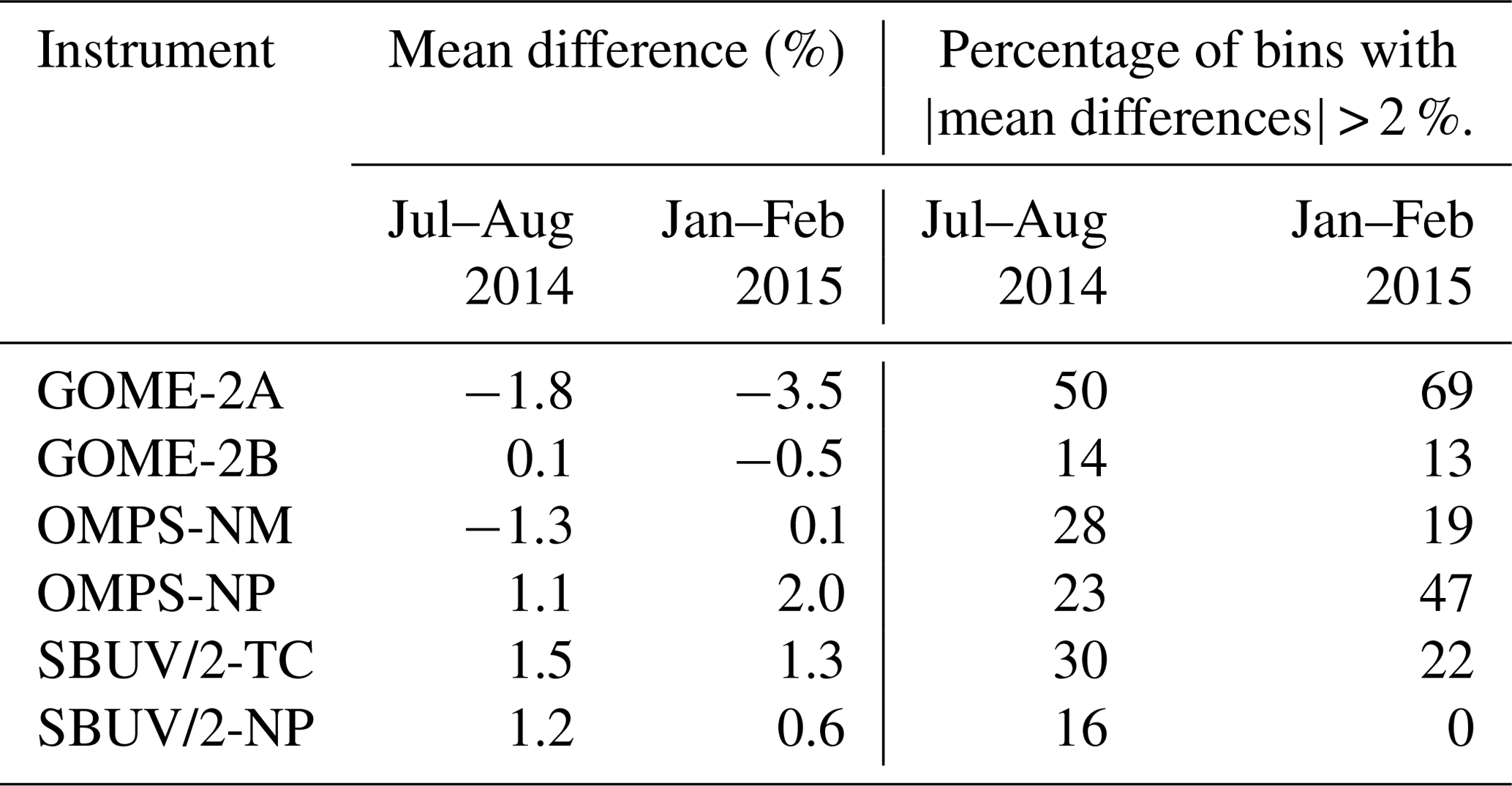
Table 2Global diagnostics of differences in total column ozone between satellite instruments and OMI-TOMS for July–August 2014 and January–February 2015. The diagnostics consists of global mean differences and percentages of non-empty SZA/latitude bins with mean differences exceeding 2 % in magnitude.
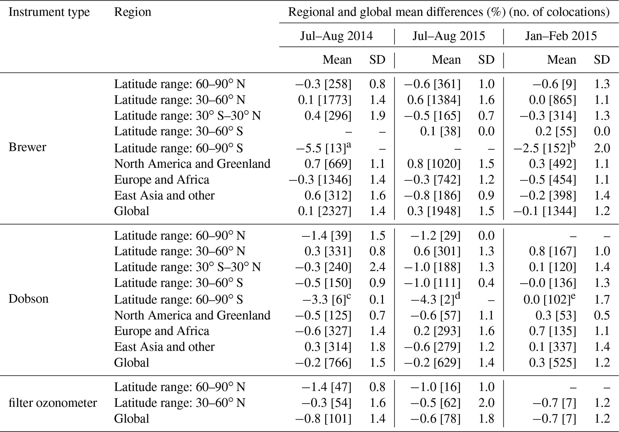
The time mean differences with OMI-TOMS for July–August 2014 and January–February 2015 are shown in Figs. 2 and 3, respectively. The figures indicate global averaged biases in the range of −3.5 % to 2 % (Table 2). The maximum time mean biases per bin reach sizes of ∼5 %–9 % for some data sets. These mean differences are in general larger than the mean differences of OMI-TOMS with ground-based data. The mean differences typically vary by roughly 3 % over the ranges of bins for SZA values lower than 70∘, while larger variations of up to ∼7 % can be seen at higher SZA values. The mean differences from SBUV/2 typically vary less between bins as compared to the other instruments. GOME-2A and GOME-2B give the largest and smallest mean differences globally, respectively. The standard errors of the mean differences shown in Figs. 2 and 3 are below 0.1 % for most bins, except for some bins at high solar zenith angles (above 70∘), due to the smaller number of colocations, where the maximum standard error found over all the data sets is 0.6 %.
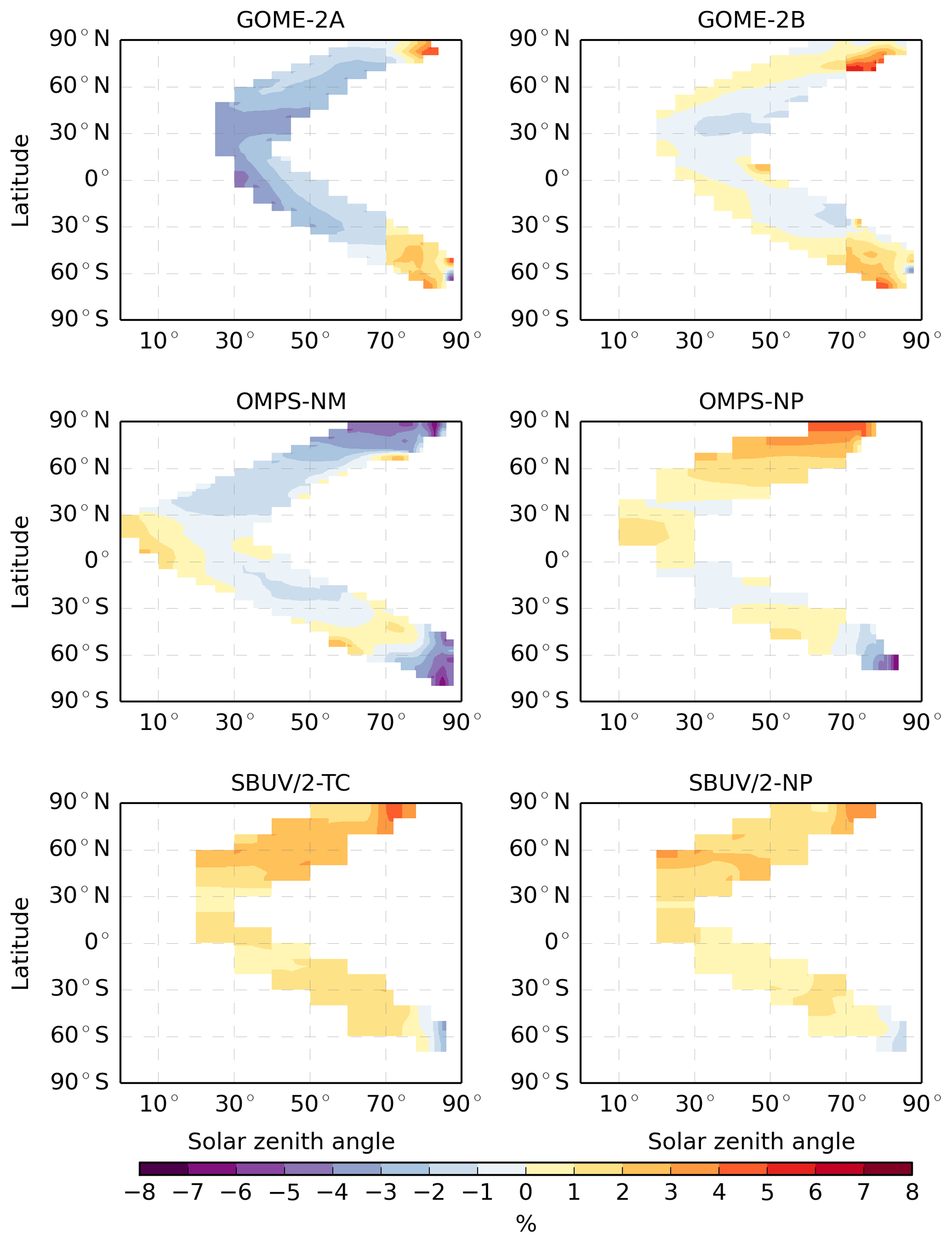
Figure 2Mean total column ozone differences (%) between GOME-2A/B, OMPS-NM/NP, SBUV/2-TC/NP and colocated OMI-TOMS data for the period of July–August 2014. The SBUV/2-TC total column ozone values stem from the two-wavelength retrieval, while those for SBUV/2-NP are the sums of the retrieved 21-layer partial columns. The colours blue to purple denote negative differences and the colours yellow to red refer to positive differences.
The discontinuity appearing at 70∘ in SZA for both GOME-2 instruments, as seen in Figs. 2 and 3, may be associated with the switch in the wavelength used to estimate reflectivity in the retrieval between lower and higher SZA from 331.3 to 360.1 nm (Table 1.13 from Zhand and Kasheta, 2009). As such, when bias corrections were applied for GOME-2, no interpolation was applied over the SZA value of 70∘.
The pattern about the Equator in Fig. 3 (January–February) appears inverted as compared to Fig. 2 (July–August) for SBUV/2 and OMPS-NP (which can also be seen in Table 3). This suggests the possibility of some seasonally dependent differences with OMI-TOMS for these instruments that may be related to changes or differences in retrieval conditions as a function of season or spectral channels as a function of solar zenith angle.
The results for the differences of the provisional OMPS-NM data with OMI-TOMS in Tables 2 and 3, considering the differences of OMI-TOMS with the ground-based data, are roughly in the same magnitude range as the differences provided in Bai et al. (2015, 2016) for the more recent OMPS-NM total column ozone products based on the SBUV V8 and V8.6 retrieval algorithms. Bai et al. (2016) provide a distribution of OMPS-NM minus OMI-TOMS values with a mean of 7.6 DU (∼2.5 % for a total column of 300 DU) and a standard deviation of 5.8 DU at the Tsukuba station (36.1∘ N, 140.1∘ E) covering the period of 2012 to early 2015. Bai et al. (2015) indicate global mean differences of OMPS-NM with ground-based data of 0.59 % for Brewer measurements and 1.09 % for Dobson measurements, with standard deviations close to 3 %. Repeating the bias-estimation exercise in this paper with the more recent products would be required for a more equitable comparison.
Table 3Mean differences of the total column ozone (%) between satellite instruments and OMI-TOMS for July–August 2014 and January–February 2015 for the Northern Hemisphere and Southern Hemisphere, for solar zenith angles below and above 70∘.
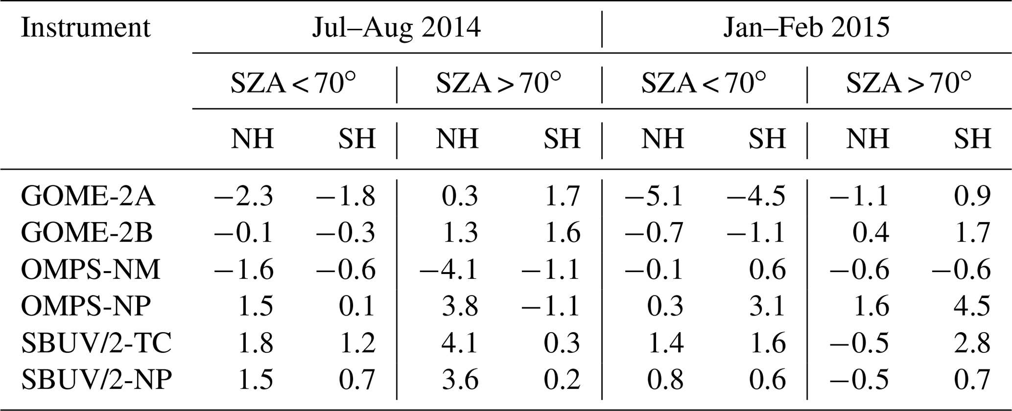
The SBUV/2-NP data set could have been an alternative candidate, as the anchor considering the temporal stability of the data quality and its level of agreement with ground-based data indicated in earlier studies. The comparisons of the SBUV/2 products with OMI-TOMS in Figs. 2 and 3 and Tables 2 and 3 suggest that OMI-TOMS may be generally closer to the ground-based data for these two periods (Table 1). OMI-TOMS also appears to be in better agreement with SBUV/2 in the Antarctic region than with the ground-based data. The agreement between OMI-TOMS and SBUV/2-NP was usually found to be slightly better than the agreement between OMI-TOMS and SBUV-TC.
The variations in time of the bias corrections for a selected single bin are shown in Fig. 4 for the July–August 2014 period. The time variations for many bins are most often within ±1 % from the time mean, but some bins can vary by ∼3 % in time. The variations in time for different instruments can differ not only in size, but also in tendency within the short 1–2-month periods.
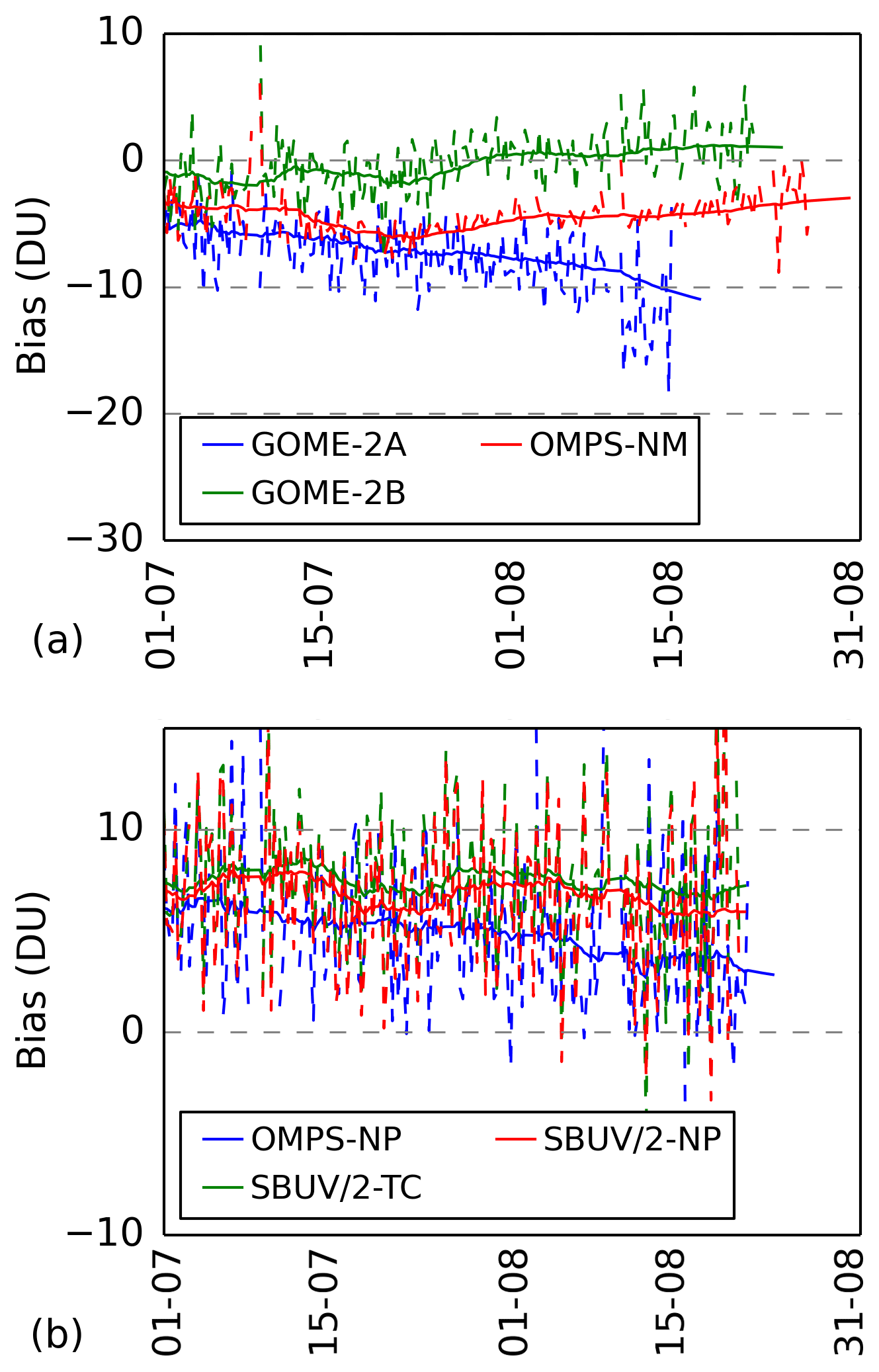
Figure 4Time series of total column ozone bias corrections (DU) for July and August 2014 for GOME-2A/B, OMPS-NM/NP, and SBUV/2-TC/NP as derived from the colocation method described in Sect. 4.1. Dashed vertical lines show individual 6 h mean differences with OMI-TOMS, while the solid curves of the same colour show the 2-week moving average bias corrections. The particular (latitude, solar zenith angle) bins plotted are 5∘ wide bins centred on (52.5∘ N, 37.5∘) for GOME-2A/B and OMPS-NM and a 10∘ wide bin centred on (55∘ N, 35∘) for OMPS-NP and SBUV/2-TC/NP. Time coverage for individual bins does not necessarily cover complete months.
4.2 Bias estimation involving differences with forecasts
An alternative bias-estimation approach utilizes the differences of the original retrieved observation data with short-term model forecasts, with the same binning in latitude and solar zenith angle averaged over a 2-week moving window. This would be applicable for near-real-time or reanalysis data assimilations. These bias estimates can be constructed by considering observation (O) differences with forecasts (F). Bias estimates can be obtained by taking the O−F differences (innovations in an assimilation context) between an instrument and a reference, which may be done with or without colocation requirements; here O denotes retrieved observations prior to bias correction. We identify three different options for this case:
- a.
with the same colocation requirements as Sect. 4.1,
- b.
without the above colocation requirements, or
- c.
〈O−F〉,
where the angular brackets denote averages and the subscript “ref” denotes differences for observations of the anchor set (OMI-TOMS for our case). Option (a) provides the potential benefit of accounting for spatial differences between paired colocation points, while options (b) and (c) bring the potential advantage of bias correction in the absence of sufficiently close colocation pairs. If previous observations of the reference or other bias-corrected instruments were assimilated into the system that produces the short-term forecasts F, then option (c) provides a bias-correction method for times or locations where the reference is not available. In this work, options (b) and (c) become successive fallback approaches to (a) in the absence of colocated anchor measurements for a bin, with option (b) automatically reducing to option (c) in the absence of the anchor data. For option (c), innovations would be of more benefit when the forecasts more strongly reflect the influence of the anchor data from previous analyses than that of the model and initial condition errors. In addition, a cutoff criterion for the use of option (c) can be imposed by requiring reference data to have been assimilated within a certain past time period to ensure that these data sets have adequate influence over the forecasts. The same binning and time averaging as done in Sect. 4.1 are used in this section.
All three of the above options for total column ozone bias estimation were performed and compared to the estimates from Sect. 4.1. Mean differences with forecasts would normally be determined and applied for bias estimation during the assimilation and forecasting cycle. For convenience, here we instead used the differences with 6 h forecasts from a separate assimilation and forecasting run (the “OMI” assimilation run summarized in Table 5), which is described in more detail in Sect. 5. In practice, the forecasts used for this approach, if applied in a near-real-time setting, would come from runs that assimilate the bias-corrected observations using the correction method considered in this section. In this section, all observational data sets used for bias estimation are thinned to 1∘, except for OMI-TOMS.
Bias estimates using options (a) to (c) above for July–August 2014 are shown in Fig. 5, which also shows the colocations-only method of Sect. 4.1 for comparison, and are summarized in Table 4. Differences between the biases resulting from options (a) to (c) and colocation alone are within 1 % over the 2-month period except for a few bins, which are mostly at high SZA, and for GOME-2A in the Southern Hemisphere also at high SZA. The standard errors of the mean differences for all cases are mostly less than 0.1 %, but can be as high as 1 % for the option (a) to (c) cases at very high SZA for bins with little data. The time evolution of these bias estimates from the 2-week moving window for two different bins is shown in Fig. 6. All bias estimates (both those that do and do not use forecast differences) follow the same general evolution in time, varying within 1 % of one another. Figure 6a, b show examples of bins that have larger and smaller evolutions in time, respectively, where for these bins the bias estimates change by ∼10 DU and ∼2–3 DU (∼3 % and ∼1 % for a total column of 300 DU), respectively.
Table 4Mean differences in total column ozone (%) between satellite instruments and OMI-TOMS for July–August 2014 using the options (a), (b), and (c) from Sect. 4.2, for the Northern Hemisphere and Southern Hemisphere and solar zenith angles below and above 70∘.
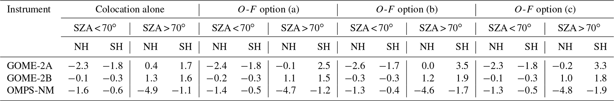
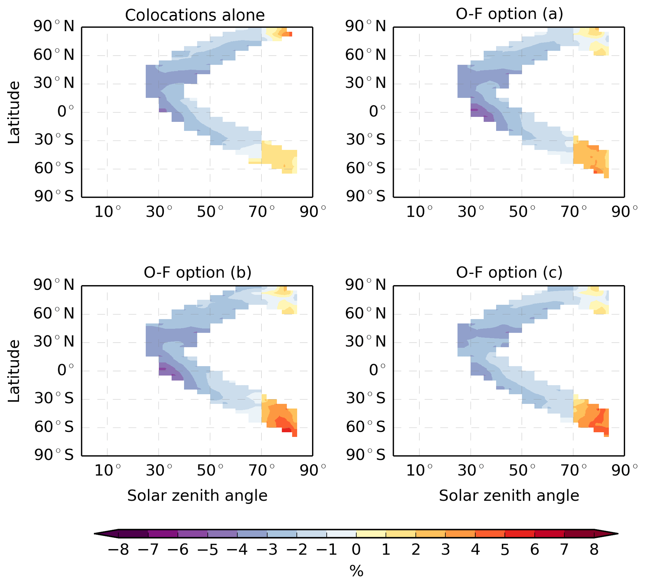
Figure 5Time mean total column ozone biases (%) between GOME-2A and OMI-TOMS for July–August 2014 from colocation alone and for the options (a), (b), and (c) of Sect. 4.2 that use observation-minus-forecast differences. For options (a), (b), and (c), the forecasts were taken from the “OMI” assimilation run (see Table 5). The bias in the “colocations alone” panel was computed using the thinned observation data set (as opposed to Figs. 2 and 3 that used the unthinned data set) to compare to the other cases that use thinned observations. The colours blue to purple denote negative differences and the colours yellow to red refer to positive differences.
The bias estimates that use differences with forecasts are largely consistent with estimates that use colocation alone. The estimates that utilize differences with forecasts can provide additional benefits over using colocations alone if the forecasts well represent the spatial variation in total column ozone for options (a) and (b) or if the forecasts have been sufficiently de-biased for option (c).

Figure 6Time series of total column ozone bias corrections (DU) for two latitude/SZA bins covering July–August 2014 for GOME-2A using different bias-correction methods. All cases that include colocation methods use thinned observation sets. The “O-F” curves additionally use the differences of forecasts described in Sect. 4.2 following the assimilation of OMI-TOMS. The “colocations alone” and “O-F” curves were calculated using the Gaussian 2-week moving average with a half width at half maximum of 4.7 d. The “Teff∕ SZA” curves, described in Sect. 4.3, result from mapping each observation that falls within the latitude/SZA bin onto the ozone effective temperature/SZA bias estimate for July–August 2014 (shown in Fig. 7), followed by taking the average of these bias estimate values for each time.
4.3 Variation with ozone effective temperature
An alternative parameterization for the bias estimation consists of using ozone effective temperature and solar zenith angle, as done in van der A et al. (2010). A motivation for a dependency on ozone effective temperature is to compensate for any unaccounted temperature sensitivity of the ozone absorption coefficients used in retrievals. In this case, bias estimation is implicitly dependent on time through temporal changes in the ozone effective temperature (and solar zenith angle). This captures at least the seasonal variations of biases associated with changes in temperature in addition to constant offsets. In this section, we briefly consider such a parameterization. For these estimates, we return to the method of Sect. 4.1, in which mean differences with OMI-TOMS are computed using only colocated observations (i.e., no use of forecasts).
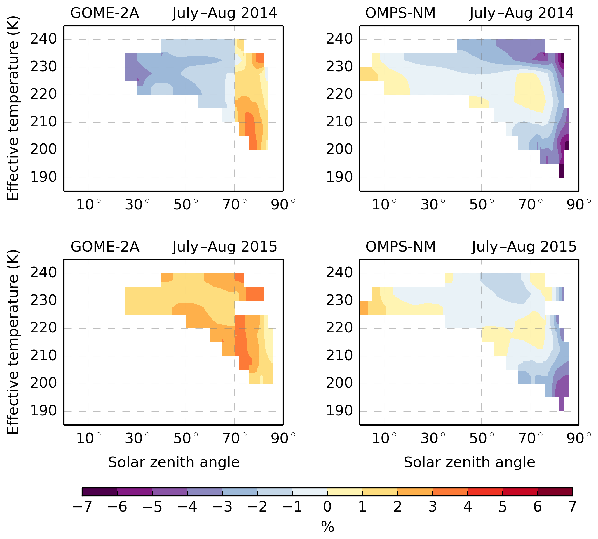
Figure 7Mean total column ozone differences (%) between GOME-2A, OMPS-NM and colocated OMI-TOMS data as a function of ozone effective temperature (Kelvin) and solar zenith angle (degrees) for the periods of July–August 2014 and July–August 2015. The colours blue to purple denote negative differences and the colours yellow to red refer to positive differences.
Ozone effective temperatures were calculated from ECCC's Global Environmental Multiscale (GEM) meteorological model, with short-term ozone forecasts driven by the linearized ozone model LINOZ. These forecasts were launched from ozone analyses that assimilated total column ozone data. Both the GEM model and ozone analyses are described in more detail in Sect. 5.
Bias estimates for GOME-2A and OMPS-NM for July–August 2014 and 2015 using an effective temperature parameterization can be seen in Fig. 7. By comparing the bias estimates for the same months from different years, we see that these bias estimates can differ notably for different time periods. With this parameterization, the bias estimate for GOME-2A differs by roughly 3 %–4 % between 2014 and 2015 for SZAs less than 70∘. These differences are larger than the long-term trends of about −2.2 DU, or roughly −0.6 % to −0.8 %, per year estimated by van der A et al. (2010) for GOME-2A (DOAS), although we note that all GOME-2 data used in this study were retrieved using the TOMS method. Differences in retrieval methods and time periods might be factors in explaining these differences. For both time periods shown in Fig. 7, applying their respective corrections results in time-averaged residual biases as a function of latitude and solar zenith angle typically within 1 %, with only a few bins over 2 % (Fig. S3).
Table 5List of assimilation experiments and their corresponding shorthand identifiers. In the second column, an asterisk (*) next to an instrument denotes that the bias-corrected observations (using the colocation method of Sect. 4.1) were assimilated.
* denotes bias-corrected observations.
An equivalent time evolution of a latitude/SZA bin can be made from the time-averaged effective temperature/SZA bias estimate shown in Fig. 7. First, the ozone effective temperature of each observation falling within a selected latitude/SZA bin is used to map that observation onto the ozone effective temperature/SZA bias estimate (Fig. 7). Then the bias estimate at each observed ozone effective temperature/SZA point is averaged for each 6 h time period. The resulting curves are shown in Fig. 6 for the selected latitude/SZA bins. The small temporal evolutions of these curves (typically well within 1 %) reflect the slight changes in the ozone effective temperature–latitude relationship in time. The greater the variation in time of the bias estimates based on the time-varying latitude/SZA parameterization, the larger the differences with the estimates based on the temperature and SZA parameterization alone (an example of which is illustrated by comparing panels (a) and (b) of Fig. 6). Overall, this supports the use of an ozone effective temperature parameterization as an alternative to latitude (and time) parameterization, with the stipulation that one accounts for any remaining notable temporal changes in some fashion when necessary.
In this section, we examine the effects of bias correction on global ozone assimilation and compare the 6 h forecasts launched from these analyses to ground-based observations and to OMI-TOMS. Corrections of observation biases were updated every 6 h using a 2-week moving window from colocations with OMI-TOMS. Assimilation experiments were conducted for July–August 2014, with a start date of 28 June 2014, 18:00 UTC, with and without bias correction. All bias-corrected observations applied in assimilation used the colocation approach without use of forecast differences (Sect. 4.1) to obtain bias estimates.
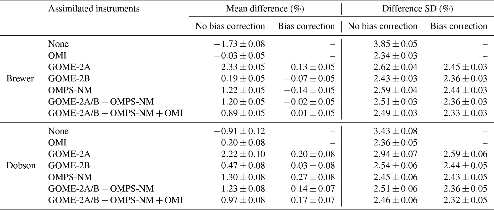
Table 6Global mean differences (%) between Brewer and Dobson total column ozone measurements and short-term forecasts for July–August 2014. For bias-corrected observations, the colocated observation bias-correction scheme (Sect. 4.1) was used. The Dobson measurements used were adjusted as a function of the ozone effective temperature (see Sect. 2.4). The uncertainties denote the standard error of the mean differences or standard deviations (SDs) of the differences. The data from the two Antarctic stations have been included here even though their mean differences with OMI are outliers relative to most mean differences (Tables S1 and S2 in the Supplement).
The forecasting model used was ECCC's GEM numerical weather prediction model (Côté et al., 1998a, b; Charron et al., 2012; Zadra et al., 2014a, b; Girard et al., 2014) coupled to the linearized ozone model LINOZ (McLinden et al., 2000; de Grandpré et al., 2016). The LINOZ model uses pre-computed coefficients generated as monthly mean climatologies to calculate the ozone production and sink contributions throughout the stratosphere and upper troposphere down to 400 hPa. A relaxation towards the climatology of Fortuin and Kelder (1998) was imposed between the surface and 400 hPa to constrain deviations away from the climatology, with a relaxation timescale of 2 days. The GEM model was executed with a 7.5 min time step with a uniform 1024×800 longitude–latitude grid and a Charney–Phillips vertically staggered grid (Charney and Phillips, 1953; Girard et al., 2014) with 80 thermodynamic levels extending from the surface to 0.1 hPa. The horizontal grid corresponds to a resolution of ∼0.23∘ in latitude and ∼0.37∘ in longitude, representing a 25 km resolution at latitude 49∘. In assimilation, inconsistencies stemming from the differences in resolutions between the model forecasts and the observations would usually be reflected by some corresponding increase in applied observation error variances. This is not explicitly done here. The vertical resolution in the upper-troposphere/lower-stratosphere (UTLS) region is in the range of 0.3 to 0.6 km, with the resolution gradually changing to ∼1.6 km at 10 hPa and 3 km at 1 hPa.
Assimilation was done using an incremental three-dimensional variational (3D-Var) approach with first guess at appropriate time (FGAT; Fisher and Andersson, 2001). This assimilation system uses components of the ECCC ensemble-variational data assimilation system (Buehner et al., 2013, 2015) adapted by the authors and Ping Du (ECCC) for constituent assimilation and was run without ensembles. The ozone background error covariances applied with this system are described in the Supplement, which has a minimum error standard deviation equivalent to ∼3 % in the mid-stratosphere. The applied observation error standard deviations assigned to all total column measurements of all sources for the conducted assimilations were set to a constant of 2 %. All assimilated total column ozone data sets, except that for OMI-TOMS, were thinned to 1∘.
The initial ozone field was an analysis from an earlier assimilation. Successive 3 h to 9 h forecasts were generated from analyses provided for 00:00, 06:00, 12:00, and 18:00 UTC synoptic times. The analyses are a composite of already available ECCC operational meteorological analyses and the ozone analyses generated from this assimilation study. Assimilation runs were compared to runs without ozone assimilation that used the same meteorological analyses as employed by the ozone assimilation runs.
Both individual and combined observation data sets were assimilated. Assimilating column ozone data from two or more sources ensures that data are continually available in the event of occasional to permanent interruption of data availability from specific instruments. For near-real-time assimilation, the interruption of the availability of the anchor data set implies the need for contingency planning for transitions of bias-correction references. One might opt to assimilate data from some sensors and monitor the data from others through comparisons with the assimilation analyses. While not necessarily negating the need for bias correction, one could always select to assimilate data from sensors with retrieval products having the smallest initial biases as compared to other products. The effects of bias correction on assimilation when separately assimilating individual and multiple sensors will be examined.
The applied evaluation metrics consist of mean differences, standard deviations, and anomaly correlation coefficients (ACCs), i.e.,
where Oi, Fi, and Ci denote the observation, forecast, and climatological values, respectively, for observation i. The ACC (see, e.g., WMO, 1992) provides a measure of the spatio-temporal correlation between the deviations of forecasts and a verifying data set (observations or analyses) from a reference (often a climatological field). For this study, the mean forecast values for the no-assimilation case over July–August 2014 were used as the reference C instead of a climatology. It was verified that substituting the 2-D ozone climatology of Fortuin and Kelder (1998) as the reference in the ACC does not significantly change the results. As anomaly correlation coefficients in assimilation typically compare forecasts with analyses instead of observations, OMI data in this case, it was also verified that both give similar results. The legends in the figures referred to in this section (Figs. 8 and 9) use the shorthand labels that denote the different assimilation runs that are described in Table 5.
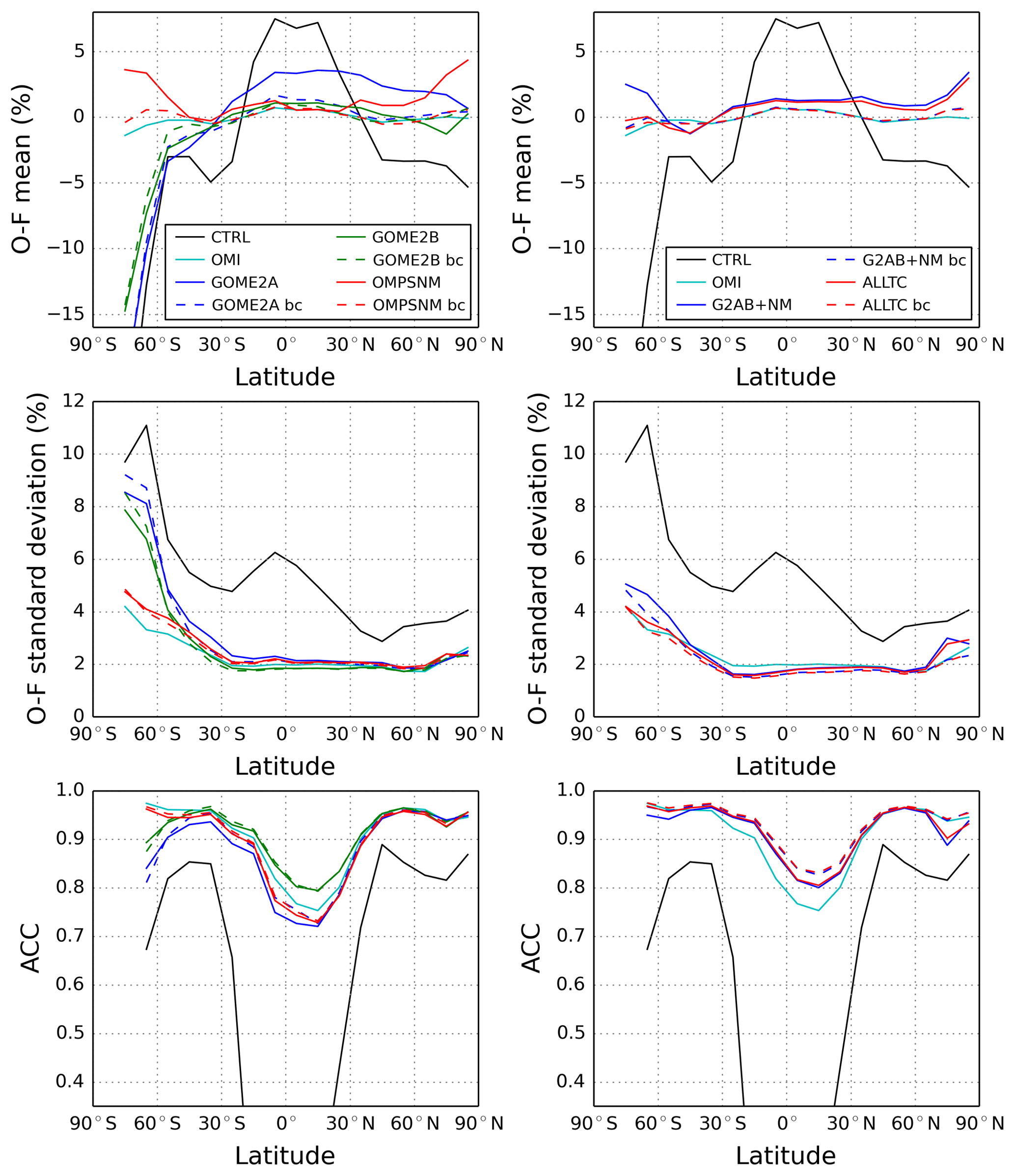
Figure 8Zonal mean total column ozone statistics of mean differences (%), standard deviations (%), and anomaly correlation coefficients (ACC; unitless) as a function of latitude (degrees) for the comparison between OMI-TOMS measurements and short-term forecasts for July–August 2014. The legends in the top plots indicate the assimilation run (see Table 5 for description) and apply to all plots in the same column.
We first examine the global differences of Brewer and Dobson total column ozone measurements with 6 h forecasts following assimilation with and without bias correction. These differences are located mostly in the northern midlatitude and tropical regions (see Fig. 1). The mean and standard deviations of these differences are shown in Table 6. Assimilating GOME-2A observations alone without bias correction actually increases the absolute size of the global mean differences relative to the no-assimilation case to over 2 %. Runs assimilating GOME-2A and OMPS-NM alone, as well as GOME-2A/B and OMPS-NM, have the global mean biases from both Brewer and Dobson reduced from above to well below 1 % when bias correction is introduced. Bias correction reduced the global mean differences to less than 0.3 % in size for all cases. Introducing ozone assimilation with and without bias correction, as compared to the no-assimilation case, reduced the standard deviations in the range of 0.5 % to 1.5 %. Introducing bias corrections results in only a small reduction of the standard deviation of differences. The remaining contributors to the standard deviation of differences include the variation of inter-station ground-based instrument calibration errors, the effect of residual bias features of the assimilated data such as from cross-track variations, and/or representativeness errors associated with the model resolution, in addition to forecast errors and random errors from the ground-based instruments.
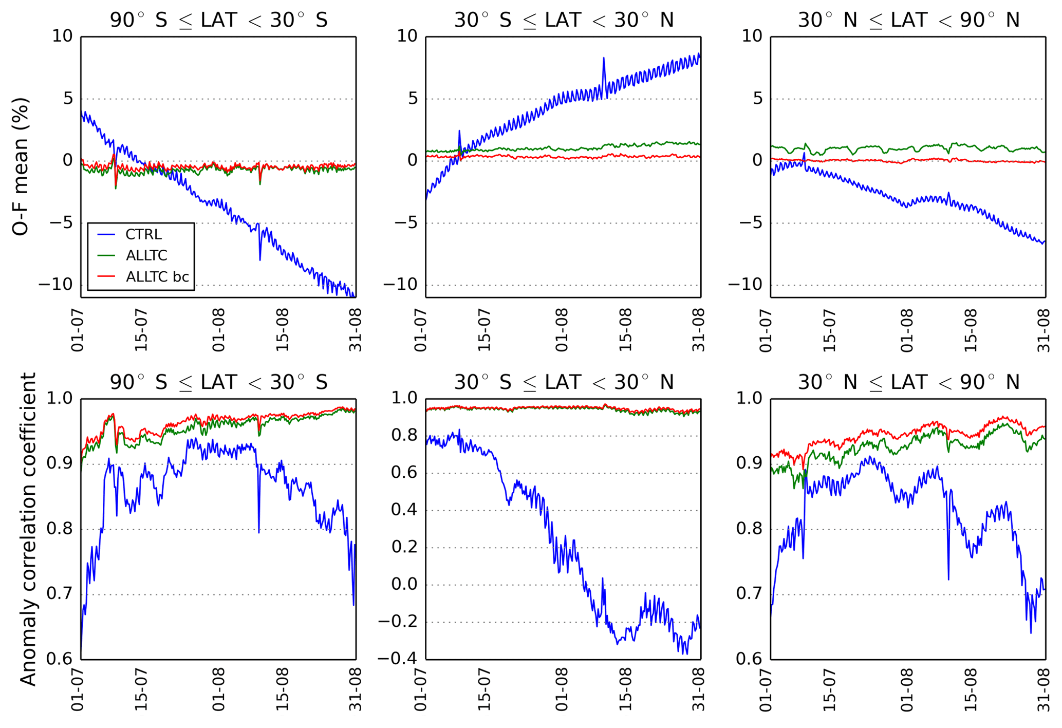
Figure 9Zonal mean differences (%) and anomaly correlation coefficients (unitless) for total column ozone between OMI-TOMS observations and short-term forecasts as a function of time (date). Results are shown for the case without assimilation as well as with the assimilation of OMI, GOME-2A/B, and OMPS-NM (both with and without bias correction). The legend indicates the assimilation run (see Table 5 for description). Each value plotted was calculated using a 24 h time window.
Comparisons of OMI-TOMS measurements with forecasts for the various experiments with and without bias correction and without any assimilation are shown in Figs. 8 and 9 for the July–August 2014 period. The GOME-2A and OMPS-NM data sets show the largest reductions in mean differences from bias correction, as would be expected from Fig. 2. The upper-left mean difference panel of Fig. 8 indicates that introducing bias correction to GOME-2A significantly increases the benefit of the GOME-2A assimilation in the tropics and northern extra-tropics. Also, the inclusion of bias correction in the assimilation of the provisional OMPS-NM data reduced the mean differences from as much as ∼4 %–5 % to within ∼1 %–2 % for the polar regions. However, assimilation over other regions and instruments mostly shows that first-order improvements stem from assimilation in general, while bias corrections result in second-order changes. Both the temporally averaged and time-varying mean differences of Figs. 8 and 9, respectively, were reduced to within 1 % over the latitude ranges where satellite data are assimilated for nearly all cases with bias correction. The exception to this is GOME-2A, which has values slightly exceeding 1 % in some places. The assimilation of bias-corrected observations from multiple sensors (labelled as “ALLTC bc”) does not notably reduce the mean differences as compared to the assimilation of individual bias-corrected sensors. Considering the earlier comparisons of forecasts with ground-based data and these results, the reduction of biases to the 1 % target appears to be achieved for the short-term forecasts in most regions where data have been assimilated.
Assimilation of total column observations improves the standard deviations of differences between the 6 h forecasts and OMI-TOMS across all latitudes, as seen in Fig. 8. Larger regional impacts in reducing standard deviations are found in the tropics and Southern Hemisphere, while there is relatively little impact from the GOME-2A/B assimilations in the southern extra-tropics, where relatively few observations are available. The large mean differences and standard deviations for GOME-2A/B assimilations below 60∘ S stem from these data sets not reaching much further south during this period. This reflects the importance of observations near the winter poles in the absence of heterogeneous chemistry in LINOZ. The impact of bias correction on the standard deviations of forecasts is not very significant.
The drift of the mean biases in time in the absence of assimilation, as seen in Fig. 9, is due to the tendency of the forecast to move toward the ozone model equilibrium state. For the GEM-LINOZ model, this results in a long spin-up period in which the ozone field moves from its initial state, based on an earlier assimilation, toward the ozone model equilibrium state. Beginning with an initial ozone field at the model equilibrium state would have increased the mean observation-minus-forecast differences and would likely not have improved the ACC of the control case, as implied by Fig. 9. Also from Fig. 9, we can see that the error of the total column ozone forecast increases by less than 5 % over the course of 15 days, reflecting the high predictability of ozone medium-range forecasts. This limited deterioration would not deter, for example, in properly forecasting the movement of low total column ozone regions during these periods.
For the ACC, forecasts from the assimilation of GOME-2B in the tropics appear better than from the assimilation of OMI-TOMS when compared to the OMI-TOMS observations. This occurs even though the OMI-TOMS data set is larger by factors of about 6 to 12 than the individual thinned data sets of the other sources. On the other hand, the GOME-2B data set, which has low biases in the tropics, provides a slightly extended longitudinal coverage over 6 h intervals, largely due to the missing strips of the OMI data set (Sect. 2.1). The ACC also demonstrates a more marked improvement in multiple sensor assimilation in the tropical region as compared to OMI-TOMS assimilation alone, which is not well seen in the mean differences. Multiple sensor assimilation with bias correction even further increases the ACC and thus the quality of the pattern and variation of the forecast fields.
Bias correction of total column ozone data from satellite instruments was performed using three different approaches. Two of the methods parameterized the bias estimation as a function of latitude, solar zenith angle, and time, while the other method used the ozone effective temperature in place of latitude and time. These approaches consisted of using observation colocation between satellite-borne instruments and a reference, referred to in this paper as the anchor. One approach also involved differences between observations and short-term forecasts. The bias estimates from the methods using the latitude/solar zenith angle parameterization were generally within 1 % of each other. The 2-month time-averaged bias estimates from the ozone effective temperature parameterization were similar to those from the other approaches. However, the lack of an explicit time dependence prevented it from capturing changes in time which, depending on the observation set and the location, could occasionally reach ∼2 %–3 % over the period of a couple of months.
The anchor used in the bias-estimation schemes was chosen as the OMI-TOMS data product, due to its wide coverage in both time and space and its good agreement with ground-based instruments. For the time periods examined in the study, OMI-TOMS was found to have global and regional mean differences with ground-based Brewer and Dobson spectrophotometers, and filter ozonometers within 1 %, except in the polar regions. Similar to larger mean differences were found between OMI-TOMS and SBUV/2 data, with OMI-TOMS generally being in better agreement with the ground-based data.
For the July–August 2014 and January–February 2015 periods, the observations based on the TOMS algorithm for the GOME-2A instrument were found to have the largest mean differences with OMI-TOMS, which could be as high as 8 % in some regions of the parameter space for solar zenith angles below 70∘. The GOME-2B instrument showed much better agreement with OMI-TOMS, with mean differences generally confined to ∼1 %–2 %, excluding at very high solar zenith angles. The provisional OMPS ozone column products, both the total column and summed partial column profile, typically had mean differences somewhere between the two GOME-2 instruments, with mean differences generally confined to ∼3 %–4 % (again excluding high solar zenith angle regions). As the quality of the different versions of OMPS-retrieved data may differ, one might expect a reduction in bias of more recent versions of the OMPS products based on the SBUV V8.6 retrieval algorithms.
It was demonstrated that the assimilation of total column ozone observations that include bias corrections as derived in this study can improve the agreement between short-term forecasts and ground-based measurements. Using a three-dimensional variational assimilation system, the assimilation of GOME-2A without bias correction gives global and time mean differences between ground-based observations and short-term ozone forecasts of ∼2.3 %. The assimilation of uncorrected OMPS-NM measurements reduced these mean differences to ∼1.3 %. Assimilating instead the bias-corrected observations brought these mean differences to well within 1 %. As a minimal global bias was found for GOME-2B, the assimilation of both corrected and uncorrected GOME-2B observations yielded mean differences within 1 %. The benefit of including total column satellite data, even without bias correction, was most notable in the tropics, in addition to the polar vortex region.
The aforementioned results indicate that the reduction of biases to within the 1 % target was achieved for most regions and cases, an exception being for conditions with high solar zenith angles. For the assimilation of two or more satellite sensors, while it is possible that the cancellation of errors from different instruments could reduce forecast biases, harmonizing the different data sets through bias correction better ensures that target reductions in residual biases are achieved. The assimilation of bias-corrected observations from multiple sensors does not notably reduce the mean differences as compared to the assimilation of individual bias-corrected sensors. However, a notable improvement in multiple sensor assimilation was seen in the tropical region as compared to OMI-TOMS assimilation alone in the anomaly correlation coefficient metric. This improvement implies an increase in the quality of the pattern and variation of the forecast fields.
The bias-estimation and bias-correction software with related shell scripts can be provided with the understanding that users will need to adapt the code to their preferred input/output data file formats. The observations can be obtained from the different centres identified in the text and the acknowledgements section below. The assimilation and forecasting system relies on ECCC computing environment tools and file conventions. Also, the computing hardware used for these assimilation cycles has since been replaced at ECCC with accompanying changes to the cycling package. References of the system components are provided in this paper. The large sets of model analyses and forecasts, and the observation-minus-forecast data sets, are saved with an in-house binary file format. Subsets could potentially be made available by the authors upon request. In addition to also containing a few complementary figures, the Supplement provides tables of station-by-station mean differences of OMI-TOMS with ground-based data related to Table 1 and Fig. 1.
The supplement related to this article is available online at: https://doi.org/10.5194/acp-19-9431-2019-supplement.
YJR directed and supervised this study, conducted some of the assimilation experiments and most of the final analyses, and is responsible for most of the manuscript text. MS significantly contributed to the manuscript text, wrote the colocation and bias-estimation and bias-correction software, conducted many of the assimilation experiments and produced the figures and the data for the tables other than for Sect. 3. Both MS and YJR contributed to the observation acquisition and preparation, and the setup of the assimilation experiments. YMC contributed to the comparison of OMI-TOMS with the ground-based data by generating the content of Tables S1–S3 and Table 1 accompanying Fig. 1. All the authors contributed to reviewing and revising the manuscript.
The authors declare that they have no conflict of interest.
The authors wish to thank Lawrence E. Flynn (NOAA) and Vitali Fioletov (ECCC) for information and advice regarding use of the different satellite data sets and the Brewer ground-based data, respectively, Jean de Grandpré and Irena Ivanova (ECCC) for the availability and assistance in use of the version of GEM with LINOZ, Ping Du and Mark Buehner (ECCC) for contributions in extending the variational assimilation code for use with constituents, Jose Garcia (ECCC) and Vaishali Kapoor (NOAA), among others associated with NOAA, for contributions in facilitating data acquisition and the various instrument teams having generated the different observation sets. Also, we are very appreciative of the contributions by the two referees toward improving the quality of this paper. We also gratefully acknowledge the following centres for access to the observations used in this paper: the National Environmental Satellite, Data, and Information Service of the National Oceanic and Atmospheric Administration (NESDIS/NOAA), the Earth Observing System Data and Information System of the National Aeronautics and Space Administration (EOSDIS/NASA), the World Ozone and Ultraviolet Radiation Data Center (WOUDC), and the Global Monitoring Division of the NOAA Earth System Research Laboratory.
This paper was edited by Ken Carslaw and reviewed by Maria-Elissavet Koukouli and one anonymous referee.
Antón, M. and Loyola, D.: Influence of cloud properties on satellite total ozone observations, J. Geophys. Res., 116, D03208, https://doi.org/10.1029/2010JD014780, 2011.
Antón, M., Loyola, D., López, M., Vilaplana, J. M., Bañón, M., Zimmer, W., and Serrano, A.: Comparison of GOME-2/MetOp total ozone data with Brewer spectroradiometer data over the Iberian Peninsula, Ann. Geophys., 27, 1377–1386, https://doi.org/10.5194/angeo-27-1377-2009, 2009a.
Antón, M., López, M., Vilaplana, J. M., Kroon, M., McPeters, R., Bañón, M., and Serrano, A.: Validation of OMI-TOMS and OMI-DOAS total ozone column using five Brewer spectroradiometers at the Iberian peninsula, J. Geophys. Res., 117, D14307, https://doi.org/10.1029/2009JD012003, 2009b.
Antón, M., Loyola, D., Clerbaux, C., López, M., Vilaplana, J. M., Bañón, M., Hadji-Lazaro, J., Valks, P., Hao, N., Zimmer, W., Coheur, P. F., Hurtmans, D., and Alados-Arboledas, L.: Validation of the Metop-A total ozone data from GOME-2 and IASI using reference ground-based measurements at the Iberian Peninsula, Remote Sens. Environ., 115, 1380–1386, https://doi.org/10.1016/j.rse.2011.01.018, 2011.
Bai, K., Liu, C., Shi, R., and Gao, W.: Comparison of Suomi-NPP OMPS total column ozone with Brewer and Dobson spectrophotometers measurements, Front. Earth Sci., 9, 369–380, https://doi.org/10.1007/s11707-014-0480-5, 2015.
Bai, K., Chang, N. B., Yu, H., and Gao, W.: Statistical bias correction for creating coherent total ozone record from OMI and OMPS observations, Remote Sens. Environ., 182, 150–168, https://doi.org/10.1016/j.rse.2016.05.007, 2016.
Bak, J., Liu, X., Kim, J. H., Chance, K., and Haffner, D. P.: Validation of OMI total ozone retrievals from the SAO ozone profile algorithm and three operational algorithms with Brewer measurements, Atmos. Chem. Phys., 15, 667–683, https://doi.org/10.5194/acp-15-667-2015, 2015.
Balis, D., Kroon, M., Koukouli, M. E., Brinksma, E. J., Labow, G., Veefkind, J. P., and McPeters, R. D.: Validation of Ozone Monitoring Instrument total ozone column measurements using Brewer and Dobson spectrophotometer ground-based observations, J. Geophys. Res., 112, D24S46, https://doi.org/10.1029/2007JD008796, 2007a.
Balis, D., Lambert, J.-C., van Roozendael, M., Spurr, R., Loyola, D., Livschitz, Y., Valks, P., Amiridis, V., Gerard, P., Granville, J., and Zehner, C.: Ten years of GOME/ERS2 total ozone data – The new GOME data processor (GDP) version 4: 2. Ground-based validation and comparisons with TOMS V7/V8, J. Geophys. Res., 112, D07307, https://doi.org/10.1029/2005JD006376, 2007b.
Bernhard, G., Evans, R. D., Labow, G. J., and Oltmans, S. J.: Bias in Dobson total ozone measurements at high latitudes due to approximations in calculations of ozone absorption coefficients and air mass, J. Geophys. Res., 110, D10305, https://doi.org/10.1029/2004JD005559, 2005.
Bhartia, P. K. and Wellemeyer, C. W.: TOMS-V8 total O3 Algorithm, Chapter 2 in: OMI Algorithm Theoretical Basis Document, Volume2, OMI Ozone Products, edited by: Bhartia, P. K., available at: http://projects.knmi.nl/omi/documents/data/OMI_ATBD_Volume_2_V2.pdf (last access: 15 July 2019), 15–31, 2002.
Bhartia, P. K., McPeters, D., Mateer, C. L., Flynn, L. E., and Wellemeyer, C.: Algorithm for the estimation of vertical ozone profiles from the backscattered ultraviolet technique, J. Geophys. Res., 101, 18793–18806, https://doi.org/10.1029/96JD01165, 1996.
Bhartia, P. K., McPeters, R. D., Flynn, L. E., Taylor, S., Kramarova, N. A., Frith, S., Fisher, B., and DeLand, M.: Solar Backscatter UV (SBUV) total ozone and profile algorithm, Atmos. Meas. Tech., 6, 2533–2548, https://doi.org/10.5194/amt-6-2533-2013, 2013.
Buehner, M., Morneau, J., and Charette, C.: Four-dimensional ensemble-variational data assimilation for global deterministic weather prediction, Nonlin. Processes Geophys., 20, 669–682, https://doi.org/10.5194/npg-20-669-2013, 2013.
Buehner, M., McTaggart-Cowan, R., Beaulne, A., Charette, C., Garand, L., Heilliette, S., Lapalme, E., Laroche, S., Macpherson, S. R., Morneau, J., and Zadra, A.: Implementation of Deterministic Weather Forecasting Systems based on Ensemble-Variational Data Assimilation at Environment Canada, Part I: The Global System, Mon. Weather Rev., 143, 2532–2559, https://doi.org/10.1175/MWR-D-14-00354.1, 2015.
Charney, J. C. and Phillips, N. A.: Numerical integration of the quasi-geostrophic equations for barotropic and simple baroclinic flows, J. Meteor., 10, 17–29, https://doi.org/10.1175/1520-0469(1953)010<0071:NIOTQG>2.0.CO;2, 1953.
Charron, M., Polavarapu, S., Buehner, M., Vaillancourt, P. A., Charette, C., Roch, M., Morneau, J., Garand, L., Aparacio, J. M., MacPherson, S., Pellerin, S., St-James, J., and Heilliette, S.: The stratospheric extension of the Canadian Global Deterministic Medium-Range Weather Forecasting System and its impact on tropospheric forecasts, Mon. Weather Rev., 140, 1924–1944, https://doi.org/10.1175/MWR-D-11-00097.1, 2012.
Chehade, W., Weber, M., and Burrows, J. P.: Total ozone trends and variability during 1979–2012 from merged data sets of various satellites, Atmos. Chem. Phys., 14, 7059–7074, https://doi.org/10.5194/acp-14-7059-2014, 2014.
Coldewey-Egbers, M., Loyola, D. G., Koukouli, M., Balis, D., Lambert, J.-C., Verhoelst, T., Granville, J., van Roozendael, M., Lerot, C., Spurr, R., Frith, S. M., and Zehner, C.: The GOME-type Total Ozone Essential Climate Variable (GTO-ECV) data record from the ESA Climate Change Initiative, Atmos. Meas. Tech., 8, 3923–3940, https://doi.org/10.5194/amt-8-3923-2015, 2015.
Côté, J., Gravel, S., Méthot, A., Patoine, A., Roch, M., and Staniforth, A.: The operational CMC–MRB Global Environmental Multiscale (GEM) model, Part I: Design considerations and formulation, Mon. Weather Rev., 126, 1373–1395, https://doi.org/10.1175/1520-0493(1998)126<1373:TOCMGE>2.0.CO;2, 1998a.
Côté, J., Desmarais, J.-G., Gravel, S., Méthot, A., Patoine, A., Roch, M., and Staniforth, A.: The operational CMC–MRB Global Environmental Multiscale (GEM) model, Part II: Results, Mon. Weather Rev., 126, 1397–1418, https://doi.org/10.1175/1520-0493(1998)126<1397:TOCMGE>2.0.CO;2, 1998b.
de Grandpré, J., Tanguay, M., Qaddouri, A., Zerroukat, M., and McLinden, C. A.: Semi-Lagrangian Advection of Stratospheric Ozone on a Yin-Yang Grid System, Mon. Weather Rev., 144, 1035–1050, https://doi.org/10.1175/MWR-D-15-0142.1, 2016.
Dee, D. P.: Bias and data assimilation, Q. J. Roy. Meteorol. Soc., 131, 3323–3343, https://doi.org/10.1256/qj.05.137, 2005.
Dee, D. P.: Importance of satellites for stratospheric data assimilation, in: Proceedings of the ECMWF Seminar on Recent developments in the use of satellite observations in numerical weather prediction, 3–7 September, ECMWF: Reading, UK, 2008.
Dee, D. P., Uppala, S. M., Simmons, A. J., Berrisford, P., Poli, P., Kobayashi, S., Andrae, U., Balmaseda, M. A., Balsamo, G., Bauer, P., Bechtold, P., Beljaars, A. C. M., van de Berg, L., Bidlot, J., Bormann, N., Delsol, C., Dragani, R., Fuentes, M., Geer, A. J., Haimberger, L., Healy, S.B., Hersbach, H., Hòlm, E. V., Isaksen, L., Kållberg, P., Köhler, M., Matricardi, M., McNally, A. P., Monge-Sanz, B. M., Morcrette, J.-J., Park, B.-K., Peubey, C., de Rosnay, P., Tavolato, C., Thépaut, J.-N., and Vitart, F.: The ERA-Interim reanalysis: configuration and performance of the data assimilation system, Q. J. Roy. Meteorol. Soc., 137, 553–597, https://doi.org/10.1002/qj.828, 2011.
Dittman, M. G., Ramberg, E., Chrisp, M., Rodriguez, J. V., Sparks, A. L., Zaun, N. H., Hendershot, P., Dixon, T., Philbrick, R. H., and Wasinger, D.: Nadir ultraviolet imaging spectrometer for the NPOESS Ozone Mapping and Profiler Suite (OMPS), Proc. SPIE 4814, Earth Observing Systems VII, 25 September 2002, Seattle, WA, edited by: Barnes, W. L., 111–119, https://doi.org/10.1117/12.453748, 2002a.
Dittman, M. G., Leitch, J., Chrisp, M., Rodriguez, J. V., Sparks, A., McComas, B., Zaun, N., Frazier, D., Dixon, T., Philbrick, R., and Wasinger, D.: Limb broad-band imaging spectrometer for the NPOESS Ozone Mapping and Profiler Suite (OMPS), Proc. SPIE 4814, Earth Observing Systems VII; 25 September 2002, Seattle, WA, edited by: Barnes, W. L., 120–130, https://doi.org/10.1117/12.453751, 2002b.
Dragani, R. and Dee, D. P.: Progress in ozone monitoring and assimilation, ECMWF Newsletter, 116, 35–42, 2008.
Durbin, P., Tilmes, C., Duggan, B., and Das, B.: OMI near real time data processing, 2010 IEEE Intern. Geoscience and Remote Sensing Symp., Honolulu, Hawaii, USA, 586–588, 25–30 July, https://doi.org/10.1109/IGARSS.2010.5651380, 2010.
Evans, R., McConville, G., Oltmans, S., Petropavlovskikh, I., and Quincy, D.: Measurement of internal stray light within 30 Dobson ozone spectrophotometers, Int. J. Remote Sens., 30, 4247–4258, https://doi.org/10.1080/01431160902825057, 2009.
Fioletov, V. E., Kerr, J. B., Hare, E. W., Labow, G. J., and McPeters, R. D.: An assessment of the world ground-based total ozone network performance from the comparison with satellite data, J. Geophys. Res., 104, 1737–1747, https://doi.org/10.1029/1998JD100046, 1999.
Fioletov, V. E., Labow, G., Evans, R., Hare, E. W., Köhler, U., McElroy, C. T., Miyagawa, K., Redondas, A., Savastiouk, V., Shalamyansky, A. M., Staehelin, J., Vanicek, K., and Weber, M.: Performance of the ground-based total ozone network assessed using satellite data, J. Geophys, Res., 113, D14313, https://doi.org/10.1029/2008JD009809, 2008.
Fisher, M. and Andersson, E.: Developments in 4-D-Var and Kalman filtering, in: Technical Memorandum Research Department, ECMWF, Reading, UK, 347 pp., 2001.
Flynn, L. (Ed.): Solar Backscatter Ultraviolet Instrument (SBUV/2) Version 8 Ozone Retrieval Algorithm Theoretical Basis Document (V8 ATBD), 45 pp., available at: https://ozoneaq.gsfc.nasa.gov/media/docs/SBUV2_V8_ATBD_020207.pdf (last access: 16 July 2019), 2 February 2007.
Flynn, L., Seftor, C., Larsen, J., and Xu, P.: Introduction to the Ozone Mapping and Profiler Suite (OMPS), in: Earth Science Satellite Remote Sensing Vol.1: Science and Instruments, edited by: Qu, J. J. et al., Springer, Berlin, 2006.
Flynn, L., Long, C., Wu, X., Evans, R., Beck, C. T., Petropavlovskikh, I., McConville, G., Yu, W., Zhang, Z., Niu, J., Beach, E., Hao, Y., Pan, C., Sen, B., Novicki, M., Zhou, S., and Sefton, C.: Performance of the ozone mapping and profiler suite (OMPS) products, J. Geophys. Res., 119, 6181–6195, https://doi.org/10.1002/2013JD020467, 2014.
Flynn, L. E., McNamara, D., Beck, C. T., Petropavlovskikh, I., Beach, E., Pachepsky, Y., Li, Y. P., Deland, M., Huang, L.-K., Long, C. S., Tiruchirapalli, R., and Taylor, S.: Measurements and products from the Solar Backscatter Ultraviolet (SBUV/2) and Ozone Mapping and Profiler Suite (OMPS) instruments, Int. J. Remote Sens., 30, 4259–4272, https://doi.org/10.1080/01431160902825040, 2009.
Fortuin, J. P. and Kelder, H.: An ozone climatology based on ozonsonde and satellite measurements, J. Geophys. Res., 103, 31709–31734, https://doi.org/10.1029/1998JD200008, 1998.
Garane, K., Lerot, C., Coldewey-Egbers, M., Verhoelst, T., Koukouli, M. E., Zyrichidou, I., Balis, D. S., Danckaert, T., Goutail, F., Granville, J., Hubert, D., Keppens, A., Lambert, J.-C., Loyola, D., Pommereau, J.-P., van Roozendael, M., and Zehner, C.: Quality assessment of the Ozone-cci Climate Research Data Package (release 2017) – Part 1: Ground-based validation of total ozone column data products, Atmos. Meas. Tech., 11, 1385–1402, https://doi.org/10.5194/amt-11-1385-2018, 2018.
Girard, C., Plante, A., Desgagné, M., McTaggart-Cowan, R., Côté, J., Charron, M., Gravel, S., Lee, V., Patoine, A., Qaddouri, A., Roch, M., Spacek, L., Tanguay, M., Vaillancourt, P., and Zadra, A.: Staggered vertical discretization of the Canadian Environmental Multiscale (GEM), Model using a coordinate of the log-hydrostatic-pressure type, Mon. Weather Rev., 142, 1183–1196, https://doi.org/10.1175/MWR-D-13-00255.1, 2014.
GOME User Manual: Product User Manual for GOME Total Columns of Ozone, NO2, tropospheric NO2, BrO, SO2, H2O, HCHO, OClO, and Cloud Properties (O3M-SAF OTO and NTO), Doc. No. DLR/GOME/PUM/01, Issue 2/E, Deutsches Zentrum für Luft und Raumfahrt e.V. – DLR, Oberpfaffenhofen, Germany, 47 pp., available at: https://earth.esa.int/c/document_library/get_file?uuid=1bca1fc9-0525-4e67-b211-b23141ce83b7&groupId=10174 (last access: 15 July 2019), 8 August 2012.
GOME-2 ATBD: Algorithm Theoretical Basis Document for GOME-2 Total Column Products of Ozone, NO2, BrO, HCHO, SO2, H2O and Cloud Properties (GDP 4.8 for O3M-SAF OTO and NTO), Doc. No. DLR/GOME-2/ATBD/01, Issue 3/A, Deutsches Zentrum für Luft und Raumfahrt e.V. – DLR, Oberpfaffenhofen, Germany, 58 pp., available at: https://wdc.dlr.de/sensors/gome2/DLR_GOME-2_ATBD_2A.pdf (last access: 15 July 2019), 30 March 2015.
Hao, N., Koukouli, M. E., Inness, A., Valks, P., Loyola, D. G., Zimmer, W., Balis, D. S., Zyrichidou, I., van Roozendael, M., Lerot, C., and Spurr, R. J. D.: GOME-2 total ozone columns from MetOp-A/MetOp-B and assimilation in the MACC system, Atmos. Meas. Tech., 7, 2937–2951, https://doi.org/10.5194/amt-7-2937-2014, 2014.
Hassinen, S., Balis, D., Bauer, H., Begoin, M., Delcloo, A., Eleftheratos, K., Gimeno Garcia, S., Granville, J., Grossi, M., Hao, N., Hedelt, P., Hendrick, F., Hess, M., Heue, K.-P., Hovila, J., Jønch-Sørensen, H., Kalakoski, N., Kauppi, A., Kiemle, S., Kins, L., Koukouli, M. E., Kujanpää, J., Lambert, J.-C., Lang, R., Lerot, C., Loyola, D., Pedergnana, M., Pinardi, G., Romahn, F., van Roozendael, M., Lutz, R., De Smedt, I., Stammes, P., Steinbrecht, W., Tamminen, J., Theys, N., Tilstra, L. G., Tuinder, O. N. E., Valks, P., Zerefos, C., Zimmer, W., and Zyrichidou, I.: Overview of the O3M SAF GOME-2 operational atmospheric composition and UV radiation data products and data availability, Atmos. Meas. Tech., 9, 383–407, https://doi.org/10.5194/amt-9-383-2016, 2016.
Inness, A., Baier, F., Benedetti, A., Bouarar, I., Chabrillat, S., Clark, H., Clerbaux, C., Coheur, P., Engelen, R. J., Errera, Q., Flemming, J., George, M., Granier, C., Hadji-Lazaro, J., Huijnen, V., Hurtmans, D., Jones, L., Kaiser, J. W., Kapsomenakis, J., Lefever, K., Leitão, J., Razinger, M., Richter, A., Schultz, M. G., Simmons, A. J., Suttie, M., Stein, O., Thépaut, J.-N., Thouret, V., Vrekoussis, M., Zerefos, C., and the MACC team: The MACC reanalysis: an 8 yr data set of atmospheric composition, Atmos. Chem. Phys., 13, 4073–4109, https://doi.org/10.5194/acp-13-4073-2013, 2013.
Kerr, J. B.: New methodology for deriving total ozone and other atmospheric variables from Brewer spectrophotometer direct sun spectra, J. Geophys. Res., 107, 4731–4747, https://doi.org/10.1029/2001JD001227, 2002.
Komhyr, W. D., Mateer, C. L., and Hudson, R. D.: Effective Bass-Paur 1985 ozone absorption coefficients for use with Dobson ozone spectrophotometers, J. Geophys. Res., 98, 20451–20465, https://doi.org/10.1029/93JD00602, 1993.
Koukouli, M. E., Balis, D. S., Loyola, D., Valks, P., Zimmer, W., Hao, N., Lambert, J.-C., van Roozendael, M., Lerot, C., and Spurr, R. J. D.: Geophysical validation and long-term consistency between GOME-2/MetOp-A total ozone column and measurements from the sensors GOME/ERS-2, SCIAMACHY/ENVISAT and OMI/Aura, Atmos. Meas. Tech., 5, 2169–2181, https://doi.org/10.5194/amt-5-2169-2012, 2012.
Koukouli, M. E., Lerot, C., Granville, J., Goutail, F., Lambert, J.-C., Pommereau, J.-P., Balis, D., Zyrichidou, I., van Roozendael, M., Coldewey-Egbers, M., Loyola, D., Labow, G., Frith, S., Spurr, R., and Zehner, C.: Evaluating a new homogeneous total ozone climate data record from GOME/ERS-2, SCIAMACHY/Envisat, and GOME-2/MetOp-A, J. Geophys. Res.-Atmos., 120, 12296–12312, https://doi.org/10.1002/2015JD023699, 2015.
Koukouli, M. E., Zara, M., Lerot, C., Fragkos, K., Balis, D., van Roozendael, M., Allart, M. A. F., and van der A, R. J.: The impact of the ozone effective temperature on satellite validation using the Dobson spectrophotometer network, Atmos. Meas. Tech., 9, 2055–2065, https://doi.org/10.5194/amt-9-2055-2016, 2016.
Kroon, M., Veefkind, J. P., Sneep, M., McPeters, R. D., Bhartia, P. K., and Levelt, P. F.: Comparing OMI-TOMS and OMI-DOAS total ozone column data, J. Geophys. Res., 113, D16S28, https://doi.org/10.1029/2007JD008798, 2008.
Labow, G. J., McPeters, R. D., Bhartia, P. K., and Kramarova, N.: A comparison of 40 years of SBUV measurements of column ozone with data from the Dobson/Brewer network, J. Geophys. Res., 118, 7370–7378, https://doi.org/10.1002/jgrd.50503, 2013.
Lahoz, W. and Errera, Q.: Constituent Assimilation, in: Data Assimilation: Making Sense of Observations, edited by: Lahoz, W., Khattatov, B. and Ménard, R., Springer-Verlag, Berlin Heidelberg, 449–490, https://doi.org/10.1007/978-3-540-74703-1_18, 2010.
Lerot, C., van Roozendael, M., Spurr, R., Loyola, D, Coldewey-Egbers, M., Kochenova, S., van Gent, J., Koukouli, M., Balis, D., Lambert, J.-C., Granville, J., and Zehner, C.: Homogenized total ozone data records from the European sensors GOME/ERS-2, SCIAMACHY/Envisat, and GOME-2/MetOp-A, J. Geophys. Res.-Atmos., 119, 1639–1662, https://doi.org/10.1002/2013JD020831, 2014.
Levelt, P. F., Joiner, J., Tamminen, J., Veefkin, J. P., Bhartia, P. K., Stein Zweers, D. C., Duncan, B. N., Streets, D. G., Eskes, H., van der A, R., McLinden, C., Fioletov, V., Carn, S., de Latt, J. DeLand, M., Marchenko, S., McPeters, R., Ziemke, J., Fu, D., Liu, X., Pickering, K., Apituley, A., González Abad, G., Arola, A., Boersma, S., Chan Miller, C., Chance, K., de Graaf, M., Hakkarainen, J., Hassinen, S., Ialongo, I., Kelipool, Q., Krotkov, N., Li, C., Lamsal, L., Newman, P., Nowlan, C., Suleiman, R., Gijsbert Tilstra, L., Torres, O., Wang., H., and Wargan, K.: The Ozone Monitoring Instrument: overview of 14 years in space, Atmos. Meas. Phys., 18, 5699–5745, https://doi.org/10.5194/acp-18-5699-2018, 2018.
Loyola, D. G., Koukouli, M. E., Valks, P., Balis, D. S., Hao, N., van Roozendael, M., Spurr, R. J. D., Zimmer, W., Kiemle, S., Lerot, C., and Lambert, J.-C.: The GOME-2 total column ozone product: Retrieval algorithm and ground-based validation, J. Geophys. Res., 116, D07302, https://doi.org/10.1029/2010JD014675, 2011.
McLinden, C. A., Olson, S. C., Hannegan, B., Wild, O., Prather, M. J., and Sundet, J.: Stratospheric ozone in 3-D models: A simple chemistry and the cross-tropopause flux, J. Geophys. Res., 105, 14653–14665, https://doi.org/10.1029/2000JD900124, 2000.
McPeters, R., Kroon, M., Labow, G., Brinksma, E., Balis, D., Petropavlovskikh, I., Veefkind, J. P., Bhartia, P. K., and Levelt, P. F.: Validation of the AURA Ozone Monitoring Instrument total column ozone product, J. Geophys. Res., 113, D15S14, https://doi.org/10.1029/2007JD008802, 2008.
McPeters, R. D., Bhartia, P. K., Haffner, D., Labow, G. J., and Flynn, L.: The version 8.6 SBUV ozone data record: An overview, J. Geophys. Res., 118, 8032–8039, https://doi.org/10.1002/jgrd.50597, 2013.
McPeters, R. D., Frith, S., and Labow, G. J.: OMI total column ozone: extending the long-term data record, Atmos. Meas. Tech., 8, 4845–4850, https://doi.org/10.5194/amt-8-4845-2015, 2015.
Moeini, O., Vaziri Zanjani, Z., McElroy, C. T., Tarasick, D. W., Evans, R. D., Petropavlovskikh, I., and Feng, K.-H.: The effect of instrumental stray light on Brewer and Dobson total ozone measurements, Atmos. Meas. Tech., 12, 327–343, https://doi.org/10.5194/amt-12-327-2019, 2019.
Munro, R., Lang, R., Klaes, D., Poli, G., Retscher, C., Lindstrot, R., Huckle, R., Lacan, A., Grzegorski, M., Holdak, A., Kokhanovsky, A., Livschitz, J., and Eisinger, M.: The GOME-2 instrument on the Metop series of satellites: instrument design, calibration, and level 1 data processing – an overview, Atmos. Meas. Tech., 9, 1279–1301, https://doi.org/10.5194/amt-9-1279-2016, 2016.
Ozone Monitoring Instrument (OMI) Near Real Time Data User's Guide, available at: https://ozoneaq.gsfc.nasa.gov/media/docs/OMI-NRT-DUG.pdf (last access: 15 July 2019), 2010.
Ozone Monitoring Instrument (OMI) Data User's Guide, produced by the OMI Team, available at: https://acdisc.gesdisc.eosdis.nasa.gov/data/s4pa/Aura_OMI_Level2G/OMTO3G.003/doc/README.OMI_DUG.pdf (last access: 15 July 2019), 62 pp., 5 January 2012.
Staehelin, J., Kerr, J., Evans R., and Vanicek, K.: Comparison of total measurements of Dobson and Brewer spectrometers and recommended transfer functions, Report No. 149, Meteorol. Org., Global Atmosphere Watch, Geneva, 2003.
Steinbrecht, W., Hegglin, M. I., Harris, N., and Weber, M.: Is global ozone recovering?, C. R. Geoscience, 350, 368–375, https://doi.org/10.1016/j.crte.2018.07.012, 2018.
van der A, R. J., Allaart, M. A. F., and Eskes, H. J.: Multi sensor reanalysis of total ozone, Atmos. Chem. Phys., 10, 11277–11294, https://doi.org/10.5194/acp-10-11277-2010, 2010.
van der A, R. J., Allaart, M. A. F., and Eskes, H. J.: Extended and refined multi sensor reanalysis of total ozone for the period 1970–2012, Atmos. Meas. Tech., 8, 3021–3035, https://doi.org/10.5194/amt-8-3021-2015, 2015.
van Roozendael, M., Peeters, P., Roscoe, H. K., De Backer, H., Jones, A. E., Bartlett, L., Vaughan, G., Goutail, F., Pommereau, J.-P., Kyro, E., Wahlstrom, C., Braathen, G., and Simon, P. C.: Validation of ground-based visible measurements of total ozone by comparison with Dobson and Brewer spectrophotometers, J. Atmos. Chem., 29, 55–83, https://doi.org/10.1023/A:1005815902581, 1998.
van Weele, M.: Ozone-cci User Requirement Document (URD), Issue 3, Reference: Ozone_cci_URD_3.0, 44 pp., available at: http://cci.esa.int/sites/default/files/filedepot/incoming/Ozone_cci_urd_v3.0_final.pdf (last access: 15 July 2019), 12 April 2016.
Veefkind, J. P. and de Haan, J. F.: DOAS Total O3 Algorithm, Chapter 3 in: OMI Algorithm Theoretical Basis Document, Volume, 2, OMI Ozone Products, edited by: Bhartia, P. K., Version 2.0, 33–50, 2002.
Veefkind, J. P., de Haan, J. F., Brinksma, E. J., Kroon, M., and Levelt, P. F.: Total ozone from the Ozone Monitoring Instrument (OMI) using the DOAS technique, IEEE T. Geosci. Remote, 44, 1239–1244, https://doi.org/10.1109/tgrs.2006.871204, 2006.
Viatte, C., Schneider, M., Redondas, A., Hase, F., Eremenko, M., Chelin, P., Flaud, J.-M., Blumenstock, T., and Orphal, J.: Comparison of ground-based FTIR and Brewer O3 total column with data from two different IASI algorithms and from OMI and GOME-2 satellite instruments, Atmos. Meas. Tech., 4, 535–546, https://doi.org/10.5194/amt-4-535-2011, 2011.
WMO (World Meteorological Organization): Manual on the global data processing system, Volume I (Annex IV to the WMO Technical Regulations), Global Aspects, Report WMO-No. 485, Secretariat of the World Meteorological Organization, Geneva, Switzerland, 1992.
Zadra, A., McTaggart-Cowan, R., Vaillancourt, P. A., Roch, M., Bélair, S., and Leduc, A.-M.: Evaluation of tropical cyclones in the Canadian Global Modeling System: Sensitivity to moist process parameterization, Mon. Weather Rev., 142, 1197–1220, https://doi.org/10.1175/MWR-D-13-00124.1, 2014a.
Zadra, A., Antonopoulos, S., Archambault, B., Beaulne, A., Bois, N., Buehner, M., Giguère, A., Marcoux, J., Petrucci, F., Poulin, L., Reszka, M., Robinson, T., St-James, J., and Rahill, A.: Improvements to the Global Deterministic Prediction system (GDPS) (from version 2.2.2 to 3.0.0), and related changes to the Regional Deterministic Prediction System (RDPS) (from version 3.0.0 to 3.1.0), available at: http://collaboration.cmc.ec.gc.ca/cmc/CMOI/product_guide/docs/lib/op_systems/doc_opchanges/technote_gdps300_20130213_e.pdf (last access: 15 July 2019), Canadian Meteorological Centre Tech. Note, 88 pp., 2014b.
Zhang, Z. and Kasheta, T.: Global Ozone Monitoring Experiment-2 (GOME-2) Operational Ozone Product System Version 8: Interface Control Document (Documentation Version 1.4), prepared for the National Environmental Satellite, Data, and Information Service (NESDIS), NOAA/NESDIS/OSPO document OSPO/ESPC-ATMO-OZGO37-01-V1.4 (last revision: September 2012, by Chen, L.), 2012.
Zhou, L., Divakarla, M., and Liu, X.: An overview of the Joint Polar Satellite System (JPSS) science data product calibration and validation, Remote Sens., 8, 139, https://doi.org/10.3390/rs8020139, 2016.
- Abstract
- Copyright statement
- Introduction
- Observations
- Evaluation of OMI-TOMS total column ozone with ground-based data
- Bias estimation and evaluation using OMI-TOMS as a reference
- Assimilation system and results
- Conclusions
- Code and data availability
- Author contributions
- Competing interests
- Acknowledgements
- Review statement
- References
- Supplement