the Creative Commons Attribution 4.0 License.
the Creative Commons Attribution 4.0 License.
 | 20 Jun 2019
Quantifying the bias of radiative heating rates in numerical weather prediction models for shallow cumulus clouds
Nina Črnivec
Bernhard Mayer
The interaction between radiation and clouds represents a source of uncertainty in numerical weather prediction (NWP) due to both intrinsic problems of one-dimensional radiation schemes and poor representation of clouds. The underlying question addressed in this study is how large the NWP radiative bias is for shallow cumulus clouds and how it scales with various input parameters of radiation schemes, such as solar zenith angle, surface albedo, cloud cover and liquid water path. A set of radiative transfer calculations was carried out for a realistically evolving shallow cumulus cloud field stemming from a large-eddy simulation (LES). The benchmark experiments were performed on the highly resolved LES cloud scenes (25 m grid spacing) using a three-dimensional Monte Carlo radiation model. An absence of middle and high clouds is assumed above the shallow cumulus cloud layer. In order to imitate the poor representation of shallow cumulus in NWP models, cloud optical properties were horizontally averaged over the cloudy part of the boxes with dimensions comparable to NWP horizontal grid spacing (several kilometers), and the common δ-Eddington two-stream method with maximum-random overlap assumption for partial cloudiness was applied (denoted as the “1-D” experiment). The bias of the 1-D experiment relative to the benchmark was investigated in the solar and thermal parts of the spectrum, examining the vertical profile of heating rate within the cloud layer and the net surface flux. It is found that, during daytime and nighttime, the destabilization of the cloud layer in the benchmark experiment is artificially enhanced by an overestimation of the cooling at cloud top and an overestimation of the warming at cloud bottom in the 1-D experiment (a bias of about −15 K d−1 is observed locally for stratocumulus scenarios). This destabilization, driven by the thermal radiation, is maximized during nighttime, since during daytime the solar radiation has a stabilizing tendency. The daytime bias at the surface is governed by the solar fluxes, where the 1-D solar net flux overestimates (underestimates) the corresponding benchmark at low (high) Sun. The overestimation at low Sun (bias up to 80 % over land and ocean) is largest at intermediate cloud cover, while the underestimation at high Sun (bias up to −40 % over land and ocean) peaks at larger cloud cover (80 % and beyond). At nighttime, the 1-D experiment overestimates the amount of benchmark surface cooling with the maximal bias of about 50 % peaked at intermediate cloud cover. Moreover, an additional experiment was carried out by running the Monte Carlo radiation model in the independent column mode on cloud scenes preserving their LES structure (denoted as the “ICA” experiment). The ICA is clearly more accurate than the 1-D experiment (with respect to the same benchmark). This highlights the importance of an improved representation of clouds even at the resolution of today's regional (limited-area) numerical models, which needs to be considered if NWP radiative biases are to be efficiently reduced. All in all, this paper provides a systematic documentation of NWP radiative biases, which is a necessary first step towards an improved treatment of radiation–cloud interaction in atmospheric models.
- Article
(8629 KB) - Full-text XML
- BibTeX
- EndNote


Despite great progress in the availability of computing power over the recent years, exact three-dimensional (3-D) radiative transfer solvers remain computationally too expensive to be routinely used in numerical weather prediction (NWP). Therefore, approximate one-dimensional (1-D) solvers are applied operationally in NWP models, introducing uncertainty into weather forecasts. The underlying assumption of 1-D solvers is the independent column approximation (ICA), where the radiative transfer problem is solved in each model column separately, thus entirely neglecting horizontal photon transport between individual columns across the model domain. As a standard technique for the solution of the radiative transfer equation within an ICA column, computationally efficient analytical two-stream methods (TSMs) are widely employed, having a laudable tradition starting more than a century ago with Schuster (1905) and Schwarzschild (1906).
A radiation parameterization scheme within a host NWP model has a two-fold task: apart from the calculation of radiative heating rate distribution within the atmosphere (K d−1) for the diabatic heating term in the prognostic temperature equation, it needs to supply the net surface radiative flux (W m−2) for the proper evaluation of the surface energy budget. While in clear-sky conditions 1-D solvers generally provide good estimates for atmospheric heating rates and surface fluxes, the error related to neglected 3-D effects considerably increases in the presence of clouds (e.g., Schmetz, 1984; O'Hirok and Gautier, 1998a, 1998b, 2004; Di Giuseppe and Tompkins, 2003, 2005; Tompkins and Di Giuseppe, 2007; Wissmeier et al., 2013).
Although the uncertainty related to the inaccurate treatment of radiation–cloud interaction in numerical models depends, inter alia, on cloud type, the present study is restricted to shallow cumulus clouds. The importance of shallow convection for the redistribution of atmospheric heat and moisture is well acknowledged (e.g., Albrecht et al., 1988, 1995; Tiedtke, 1989; Zhao and Austin, 2005). Small-scale fluctuations in microphysical, dynamical and thermodynamical parameters observed in boundary layers containing cumuli (Baker et al., 1985) indicate the complexity of a proficient coupling of cumulus cloud fields with a full 3-D radiative field.
In the last decades, large-eddy simulation (LES) and cloud-resolving models (CRMs) models have become an important tool in boundary layer research (Neggers et al., 2003). If an accurate 3-D radiation (e.g., Monte Carlo) calculation is performed on such 3-D highly resolved cumulus clouds (“benchmark experiment” or “truth”), the following is observed. In the solar spectral range, the largest heating is at the illuminated cloud side, and the shadow of the cloud at the ground is shifted according to solar zenith angle (Wapler and Mayer, 2008; Wissmeier et al., 2013; Jakub and Mayer, 2015, 2016). In the thermal spectral range, there is a strong cooling of cloud top and cloud sides and modest warming of cloud bottom (Kablick III et al., 2011; Klinger and Mayer, 2014, 2016). In the associated ICA calculation, the 3-D effects related to cloud sides are misrepresented; the main shortcomings are as follows. In the solar spectral range, the heating is always at cloud top and the shadow at the surface lies directly underneath the cloud, which is fundamentally wrong unless the Sun is at zenith (Jakub and Mayer, 2015, 2016). In the thermal spectral range, the ICA approximation only captures cloud top cooling and cloud base warming but entirely neglects the cooling of cloud sides (Kablick III et al., 2011; Klinger and Mayer, 2014, 2016).
When 3-D radiation parameterizations are coupled to an LES or CRM model, the abovementioned shortcomings of ICA on the cumulus cloud evolution can be studied. Klinger et al. (2017) showed that interactive 3-D thermal radiation affects cloud circulation by enhancing cloud-core updrafts and surrounding subsiding shells. In addition, it alters the organization of clouds (i.e., convective self-aggregation). In a recent study by Jakub and Mayer (2017), it was shown that interactive 3-D solar radiative transfer may cause formation of cloud streets similar to the known roll clouds caused by wind shear, whereas the ICA approximation produces randomly positioned clouds.
Before these effects can be directly simulated within NWP, we are presumably at least a decade away from the desired resolution. Today's regional NWP models with horizontal grid spacing on the order of few kilometers (e.g., the operational model of German Weather Service in its convection-permitting configuration COSMO-DE with horizontal grid spacing of 2.8 km) mostly resolve deep convection and have a parameterization for shallow convection. Depending on cloud parameterization scheme, subgrid-scale cloudiness (cloud fraction) within a model grid box is usually diagnosed from the grid-scale relative humidity. Shallow cumulus clouds in state-of-the-art NWP are thus represented as horizontally homogeneous layers of partial cloudiness, entirely missing their 3-D geometrical structure and small-scale variability of optical properties. Further, an assumption is required of how partial cloudiness is distributed in the vertical direction, which is another deficiency of NWP radiation schemes (e.g., Barker et al., 2003; Barker, 2008; Wu and Liang, 2005; Kablick III et al., 2011). The widely employed assumption is the maximum-random overlap assumption (Geleyn and Hollingsworth, 1979), which, implemented in the two-stream framework, gives the so called two-stream method with maximum-random overlap assumption for partial cloudiness (Ritter and Geleyn, 1992), commonly used as the NWP radiation solver.
To summarize, the interaction between radiation and shallow cumulus clouds represents a source of uncertainty in NWP due to both intrinsic problems of 1-D radiation schemes and poor representation of subgrid-scale clouds. The underlying question of the present study is as follows: how large is the bias of NWP radiative heating rates on shallow cumulus clouds, and how does it scale with various input parameters of radiation schemes, such as solar zenith angle (SZA), surface albedo (A), total cloud cover (CC) and cloud liquid water path (LWP)?
This paper is organized as follows. The experimental design is outlined in Sect. 2, whereas in Sect. 3 the results are presented. Summary and concluding remarks are given in Sect. 4.
First, in Sect. 2.1, the Monte Carlo radiation model, which is used for the 3-D benchmark and ICA calculations, is introduced. Then, in Sect. 2.2, we describe the δ-Eddington two-stream method with maximum-random overlap assumption for partial cloudiness as employed in this study. In the subsequent section (Sect. 2.3 and 2.4), the cloud field data set and the related experimental strategy are presented. Finally, the general setup of radiative transfer computations is summarized in Sect. 2.5.
2.1 Reference model – MYSTIC
The benchmark experiments are performed with the 3-D radiative transfer model MYSTIC, the Monte Carlo code for the physically correct tracing of photons in cloudy atmospheres (Mayer, 2009), which is part of the libRadtran software package (http://www.libradtran.org/doku.php, last access: 10 April 2019; Mayer and Kylling, 2005; Emde et al., 2016) and can be run in independent column mode as well. MYSTIC participated in both phases of the international Intercomparison of 3-D Radiation Codes (I3RC; Cahalan et al., 2005), where it proved its ability to accurately compute radiative transfer in versatile cloud scenarios.
2.2 δ-Eddington two-stream method with maximum-random overlap assumption for partial cloudiness
We begin by introducing the classic δ-Eddington two-stream method (Joseph et al., 1976) suitable for a horizontally homogeneous model atmosphere and then explain the extension of this method which accounts for partial cloudiness.
The common feature of two-stream methods is the division of the radiation field into direct (unscattered) solar beam (S) and two streams of diffuse radiation – the downward (E↓) and upward (E↑) components. For most applications, δ-TSMs, in which a part of the scattered radiation is retained in the direct beam to approximate the strong forward-scattering peak of cloud droplets and aerosol particles, have been found to be more accurate than two-stream methods without δ scaling (Räisänen, 2002). The fractional scattering into the forward peak taken to be the square of the phase function asymmetry parameter is what distinguishes the widely used δ-Eddington approximation from others of similar nature.
For the calculations in a vertically inhomogeneous atmosphere, the atmosphere is discretized into a number of homogeneous layers, each characterized by its optical properties (optical thickness, single scattering albedo, asymmetry parameter). Consider first a single layer (j) located between levels (i−1) and (i) 1. A system of linear equations determining the fluxes that emanate from this layer as a function of fluxes that enter the layer can be written in matrix form as
The linear coefficients akl in Eq. (1), referred to as Eddington coefficients, are functions of optical properties of layer (j). They have the following physical meaning: a11 and a12 represent the transmission and reflection coefficient for diffuse radiation, respectively. Further, a13 and a23 represent the reflection and transmission coefficient for the primary scattered solar radiation, respectively, while a33 denotes the transmission coefficient for the direct solar radiation. For the details of their definitions, as well as for the inclusion of thermal radiation, the reader is referred to Zdunkowski et al. (2007).
In a consecutive step, individual layers are concatenated by imposing flux continuity at each level. Taking appropriate boundary conditions at the top of the atmosphere (TOA) and at the ground into account, the equation system is solved analytically by means of standard numerical procedures (e.g., Zdunkowski et al., 2007; Stephens and Webster, 1981; Ritter and Geleyn, 1992; Stephens et al., 2001). After radiative fluxes throughout the atmosphere have been computed, the calculation of heating rates is straightforward. The heating rate (K d−1) of an individual layer is given by
where ρ represents air density, cp represents the specific heat capacity of air at constant pressure, Δz represents the vertical thickness of the layer, and ΔEnet represents the radiative flux absorbed in the layer (W m−2), defined as the difference between the fluxes entering the layer and those leaving the layer.
Consider now a partially cloudy layer (Fig. 1a), which is characterized by two sets of optical properties and corresponding Eddington coefficients – one for the cloudy region (superscript c) and the other for the cloud-free region (superscript f). In order to apply the maximum-random overlap assumption (Geleyn and Hollingsworth, 1979), the cloudy and cloud-free fluxes need to be treated separately. Total radiative flux at a given level is thus the sum of the cloudy and cloud-free components, e.g.,
and analogously for both diffuse components. The equation system (1) is replaced by
so that the fluxes emanating from the cloudy and cloud-free regions depend on a linear combination of both cloudy and cloud-free incoming fluxes. Overlap coefficients p1, p2, p3 and p4 refer to layer (j) and describe the division of incoming fluxes between the cloudy and cloud-free regions in accordance with the maximum-random overlap assumption, where adjacent cloudy layers are overlapped maximally, and cloudy layers separated by at least one cloud-free layer are overlapped randomly. For layer (j), they have the following form:
with C representing layer cloud fraction. Figure 1b, c illustrate both possible geometries that need to be considered in order to determine the coefficients p1 and p3 related to the division of downward fluxes (the division of upward fluxes is managed via p2 and p4 in a similar fashion). The method has been successfully implemented in the radiative transfer package libRadtran for the purpose of this study.
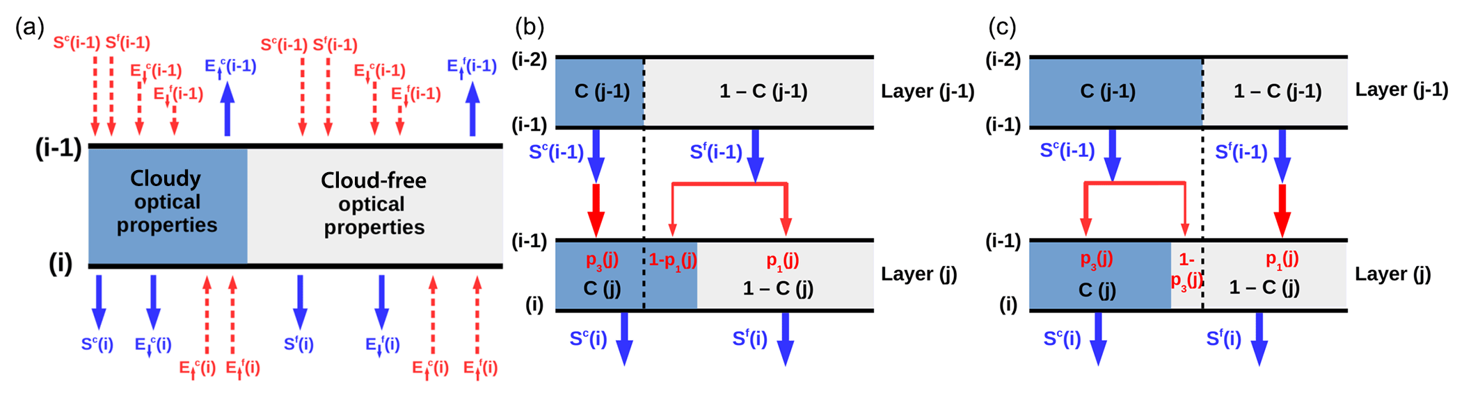
Figure 1(a) Schematic of a partially cloudy model layer located between levels (i−1) and (i), which has the information about the cloudy and cloud-free optical properties. The blue arrows represent radiative fluxes emanating from cloudy and cloud-free regions. The red arrows indicate a complex situation of possible incoming fluxes, which can though be determined taking the overlap rules and knowledge about the cloud fraction in the adjacent layers into account. Panels (b) and (c) illustrate the transmission of direct solar radiation through two adjacent layers with different cloud fraction for maximum overlap concept. Panel (b) shows the situation where the upper layer has smaller cloud fraction than the lower layer, while (c) shows the opposite situation.
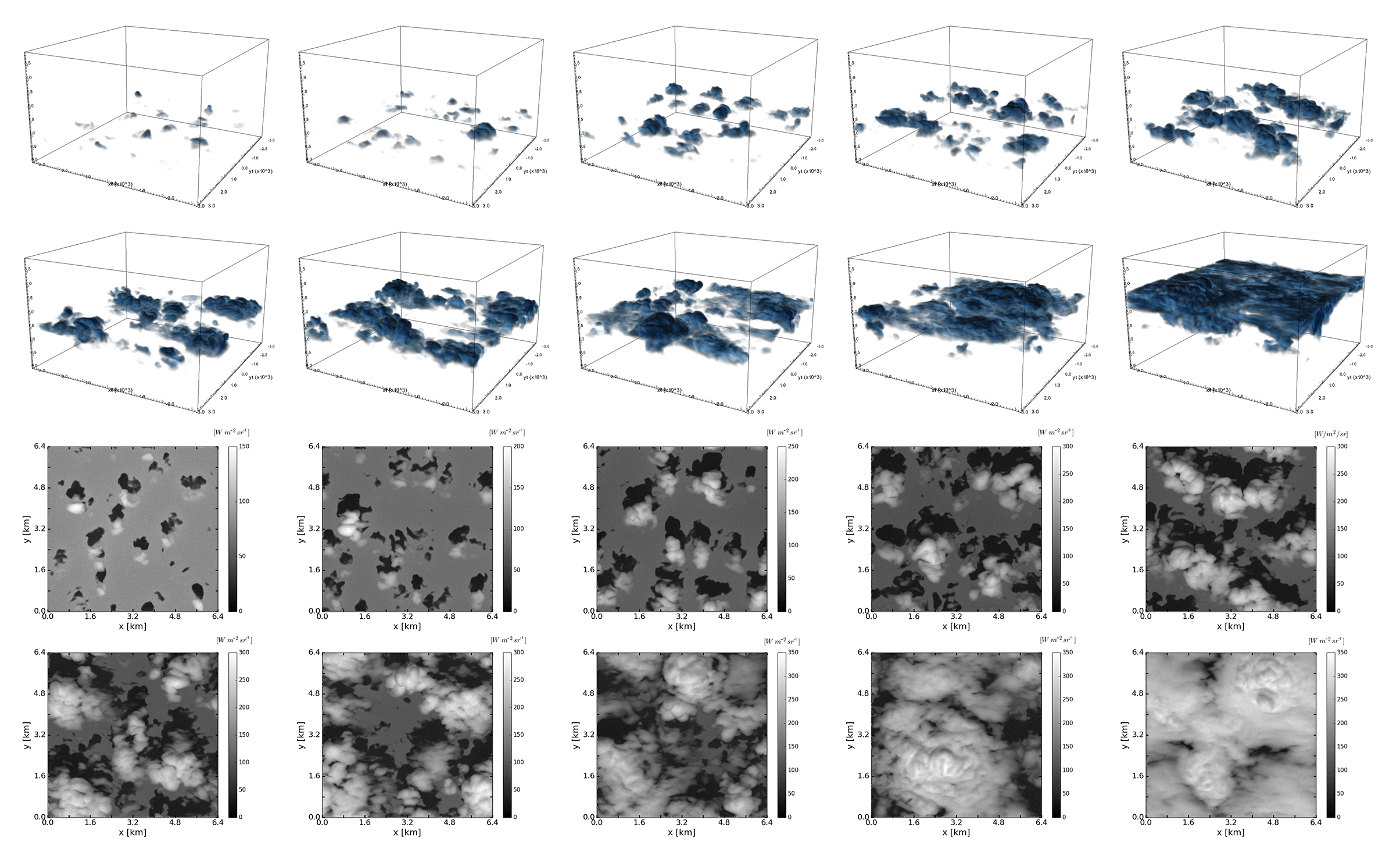
Figure 2A set of shallow cumulus cloud scenes used as input for radiative transfer calculations. Top – visualization with VisIt. Bottom – visualization with the 3-D radiative transfer model MYSTIC (Mayer, 2009); shown is nadir radiance distribution at a height of 5 km with the Sun under a zenith angle of 30∘ illuminating the scenes from the south.
2.3 Cloud field data set
Input for offline radiation calculations is a set of shallow cumulus cloud fields, simulated with the University of California, Los Angeles large-eddy simulation (UCLA-LES) model. The simulation relates to the Rain in Cumulus over the Ocean (RICO; Rauber et al., 2007) experiment. The horizontal domain size is 6.4×6.4 km2, with the vertical extent of the domain being 4 km. A constant model grid spacing of 25 m is used in all three (x, y, z) directions. A 3-D distribution of cloud liquid water content (LWC) is extracted from the simulation run and the corresponding effective radius (Re) is assigned to each LWC value following Bugliaro et al. (2011) (see their Eq. 1 in Sect. 3.1.3). For our analysis, we choose a set of 10 cloud scenes (depicted in Fig. 2) from the initial 8 h of simulation in a way that total cloud cover of the scene varies between ∼10 % and ∼100 % with a step of approximately 10 %. Thus, the set comprises examples of broken cumulus as well as more uniform stratocumulus clouds. These cloud scenes have highly variable optical thicknesses, with maximum vertically integrated optical thicknesses of ∼20, ∼80 and ∼230 corresponding to scenes with total cloud cover of ∼10 %, ∼50 % and ∼100 %, respectively.
2.4 Strategy
To assess the bias of NWP radiative quantities, an NWP-type experiment together with a benchmark is required. The benchmark calculation using MYSTIC was performed on a cloud field preserving its LES resolution, with the result horizontally averaged over the domain (hereafter abbreviated as the “3-D” experiment). In order to mimic the poor representation of shallow cumulus in NWP models and thus create a proper NWP-type experiment, the information content of the cloud field needs to be reduced. Therefore, LWC and Re were horizontally averaged over the cloudy part of the boxes with dimensions comparable to NWP horizontal grid spacing (3.2 km). In this way, four NWP-sized boxes which generally contain partial cloudiness were created in each vertical layer (Fig. 3b) and the δ-Eddington two-stream method with maximum-random overlap assumption was called four times per cloud scene. The resulting radiative quantities were again horizontally averaged over the domain (hereafter abbreviated as the “1-D” experiment). Moreover, it should be noted that the resolution of the cloud field in the 1-D experiment was only degraded in the horizontal plane, whereas the vertical resolution was kept the same as inherited from the LES grid (25 m). 2 In summary, the 1-D experiment has multiple error sources, namely, the poor horizontal cloud structure and vertical overlap assumption, as well as the neglected grid-scale and subgrid-scale horizontal photon transport.
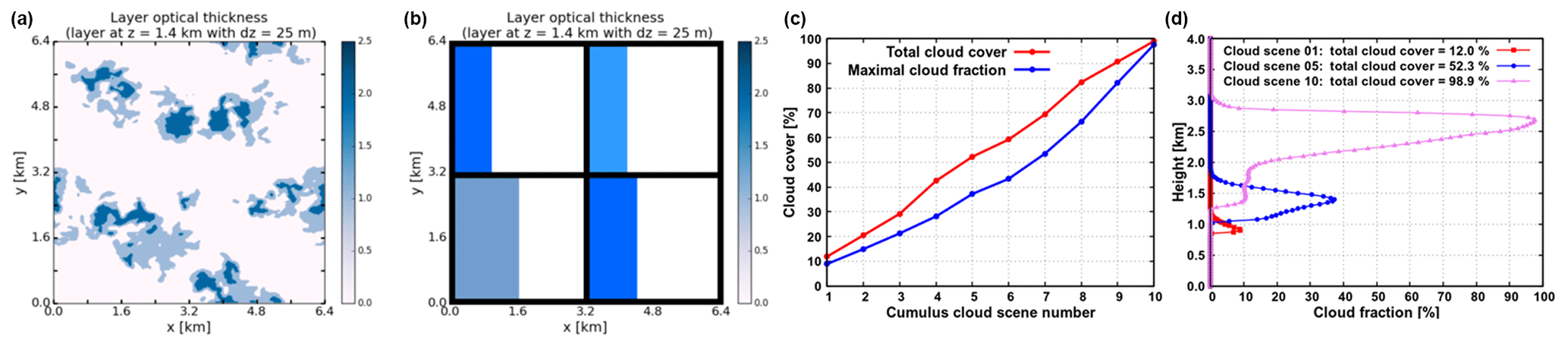
Figure 3Strategy trailing the definitions of the experiment trio (3-D, 1-D, ICA). Panel (a) shows layer optical thickness of LES cloud field, which is used as input for the 3-D and ICA experiments (shown is an example layer at a height of 1.4 km of the cloud scene with total cloud cover of 52.3 %). Panel (b) illustrates the division of this layer into four NWP-sized boxes with horizontal dimension of 3.2 km, each containing a horizontally homogeneous cloud, constructed by averaging LES distributions of LWC and Re over the cloudy fraction of the box. Applying this procedure in each vertical layer creates four columns with partial cloudiness, which resemble conditions in NWP models and serve as input for the two-stream method with maximum-random overlap assumption. Panel (c) shows total cloud cover versus maximal layer cloud fraction for the entire set of 10 cumulus cloud scenes. The discrepancy between the two curves is a measure of the erroneousness of the maximum-random overlap assumption. Panel (d) shows vertical profiles of cloud fraction for the three selected cloud scenes with total cloud cover of 12.0 %, 52.3 % and 98.9 %.
Furthermore, we created a third, intermediate experiment by running MYSTIC in independent column mode on a cloud field preserving its LES resolution and again averaging the result horizontally over the domain in the final step (hereafter abbreviated as the “ICA” experiment). The ICA experiment is thus the same as the 3-D experiment except that it neglects horizontal photon transport between the LES-grid columns. In this way, we are able to isolate and quantify the contribution of neglected horizontal photon transport to the overall error of 1-D experiments (in the hypothetical case when the subgrid-scale cloud structure would be perfectly guessed).
For each of the three experiments, we diagnosed the radiative heating rate within the cloud layer and net surface flux (i.e., difference between the total downward and upward surface flux). The error is given by the absolute and relative bias and the root mean square error (RMSE):
where denotes the result of either the 1-D or the ICA experiment and denotes the result of the 3-D experiment.
2.5 Radiative transfer computations – model setup
Each trio of experiments (3-D, 1-D, ICA) was repeated for each cloud scene in both the solar and thermal spectral range. Three-dimensional distributions of LWC and Re were converted into optical properties using the parameterization of Hu and Stamnes (1993), which uses the Henyey–Greenstein phase function as an approximation of the real Mie phase function. The background profiles of atmospheric pressure, temperature, density and trace gases (water vapor, O3, CO2) were taken from the US standard atmosphere (Anderson et al., 1986) and are horizontally homogeneous across the domain. Parameterization of absorption and scattering properties of the atmosphere in the solar part of the spectrum follows the correlated-k distribution of Kato et al. (1999). Parameterization of molecular absorption in the thermal spectral range was adopted from Fu and Liou (1992). Solar zenith angle was varied from 0∘ (overhead Sun) to 80∘ with a step of 10∘, while solar azimuth angle was held fixed at 0∘ (i.e., Sun illuminating the cloud scenes from the south). Further, we varied the surface shortwave albedo by applying constant values of 0.25 and 0.05 as typical high and low values representing land and ocean. In the thermal part of the spectrum, the surface was assumed to be non-reflective. In the Monte Carlo calculations in the solar spectral range, we applied a standard forward photon tracing method, starting a total number of 65 536 000 photons (1000 photons per LES-grid column) at TOA. In the thermal spectral range, the backward photon tracing method of Klinger and Mayer (2014) was used and 1000 photons were required in each LES-grid box of the cloud layer.
First, in Sect. 3.1 and 3.2, we present atmospheric heating rates and surface fluxes as a function of SZA in the experiments on a single cloud scene with an intermediate cloud cover of 52.3 % placed over land. In the subsequent section (Sect. 3.3, 3.4 and 3.5) additionally the dependence on surface albedo, cloud cover and liquid water path is discussed.
3.1 Heating rate in the cloud layer
The vertical profile of radiative heating rate influences atmospheric stratification and directly impacts flow dynamics. Figure 4 shows the vertical profile of radiative heating rate in the trio (3-D, 1-D, ICA) of experiments in the solar spectral range for SZAs of 0, 30 and 60∘, as well as in the thermal spectral range. In order to highlight the effects of clouds on radiative biases, we examine only the profiles within the cumulus cloud layer, which is located between 1.025 and 1.875 km height (the cloud-free atmosphere below and above these heights is not shown). In the solar 3-D experiment for overhead Sun (Fig. 4a), there is strong absorption of solar radiation in the cloud layer, resulting in a peak heating rate of about 9 K d−1 reached at approximately 1.5 km height. This is slightly above the height of maximum cloud fraction (1.4 km) due to the fact that cloud liquid water, which is the dominant absorber of solar radiation in this layer, generally increases with height from cloud base towards cloud top (except in the uppermost region of the cloud, where it decreases with height due to entrainment). The maximum heating rate is thus located between the height of maximum cloud fraction and the height of maximum LWC. As the Sun descends, the incoming radiation at TOA decreases with the cosine of SZA and so does the solar heating rate in the cloud layer, reaching a maximum value of about 8 K d−1 at SZA of 30∘ and about 5 K d−1 at SZA of 60∘ in the 3-D experiments. The height where the maximum heating is reached stays approximately the same for all SZAs. In the thermal spectral range, the cloud layer is subjected to strong cooling, attaining a peak value of about 13 K d−1 again at a height of ∼1.5 km. Below this height, the magnitude of cooling decreases towards the cloud base, where a slight cloud base warming effect is observed.
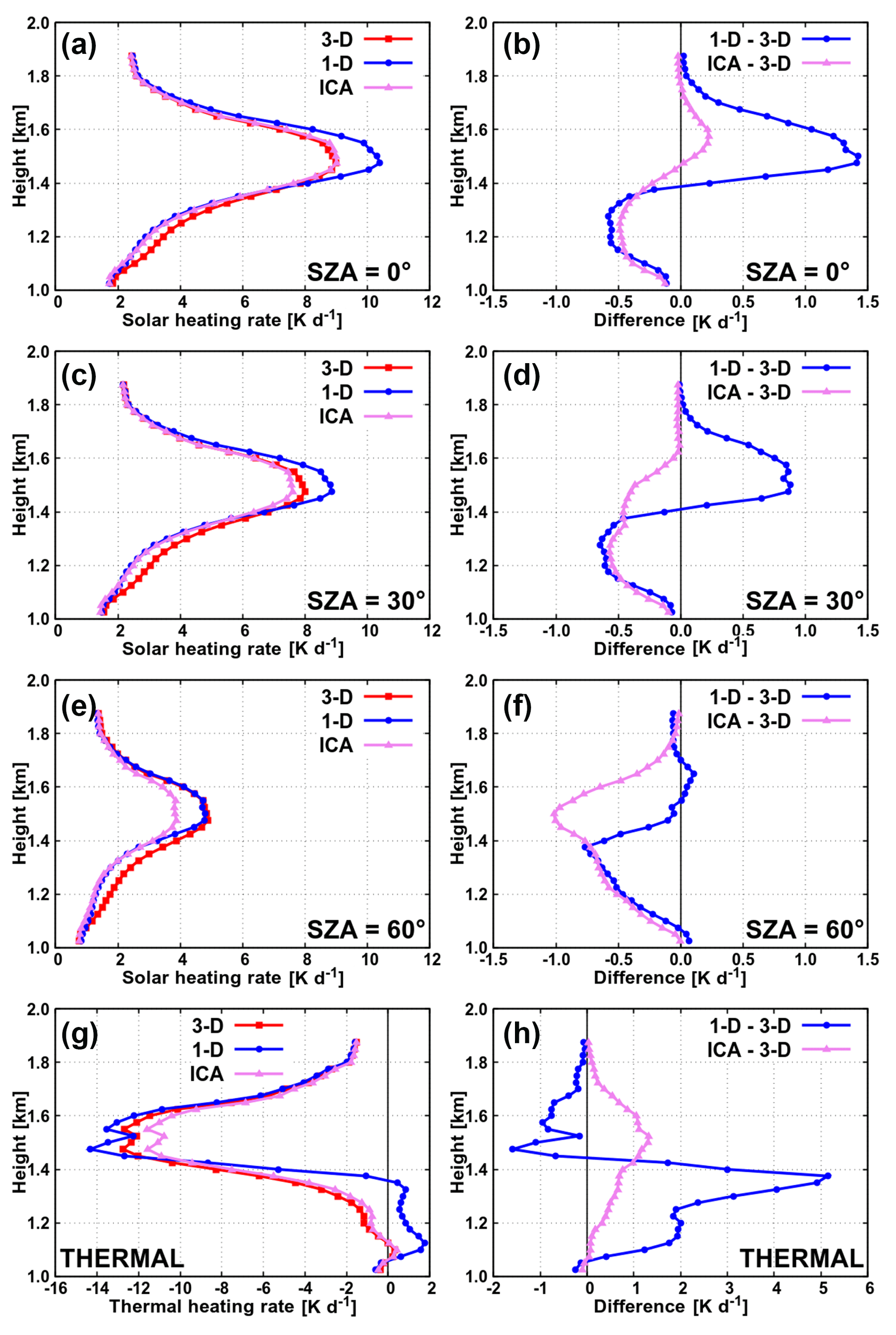
Figure 4Heating rate in the cloud layer of cumulus cloud scene with total cloud cover of 52.3 % in the experiments with land albedo.
The difference between the 1-D experiment and the 3-D benchmark (Fig. 4b, d, f, h) is as described in the following: in the solar experiments at high Sun (SZA between 0 and 50∘), the bias of the 1-D profile shows pronounced vertical gradient within the cloud layer and changes its sign approximately at a height of maximum cloud fraction. In the top part of the cloud layer (i.e., above maximum cloud fraction), the 1-D solar heating rate is too high, while in the bottom part of the cloud layer it is too low, compared to the 3-D heating rate. In the case of low Sun (SZA of 60∘ and larger), the 1-D solar heating rate is systematically too low compared to its 3-D counterpart throughout the entire cloud layer. The main reason for that is cloud side illumination (Jakub and Mayer, 2015, 2016), which is taken into account in 3-D experiments and is completely absent in 1-D calculations.
The ICA calculations help to explain these findings. In the case of overhead Sun, the amount of radiative energy hitting cloud tops is practically the same in both ICA and 3-D experiments, yet in the 3-D experiment some of the photons escape through cloud sides (an effect known as “cloud side escape or loss of photons”; O'Hirok and Gautier, 1998a; Hogan and Shonk, 2013), whereas in the ICA approximation the photons remain trapped within individual atmospheric columns. As a consequence, the ICA heating rate is larger than the 3-D heating rate within the top part of the cloud layer (Fig. 4a, b). This leakage of photons through cloud sides in the 3-D configuration simultaneously leads to an increased radiation component reaching the ground and being reflected back towards the cloud, which increases the absorption in the bottom part of the cloud layer. For this reason, within the bottom part of the cloud layer, the 3-D heating rate is larger than the ICA one. With increasing SZA, the 3-D cloud side illumination effect becomes increasingly more important (overcoming the loss of photons through cloud sides in the upper layers) and the ICA heating rate is found to be systematically too low throughout the entire vertical extent of the cloud layer (at SZA of 30∘ and larger).
A thorough inspection of the solar experiments in Fig. 4 reveals that the 1-D profiles almost completely match the ICA ones in the bottom part of the cloud layer, while in the top part of the cloud layer there is a large discrepancy between the two (at all SZAs). This suggests that “classic 3-D radiative effects” related to horizontal photon transport (discussed above in terms of the difference between ICA and 3-D) can explain the bias of 1-D profiles in the bottom part of the cloud layer (and are thus presumably by far the largest contributor to the overall bias of 1-D profiles in this region). In the top part of the cloud layer, however, the additional error sources accompanying the 1-D experiment, namely the misrepresentation of cloud horizontal heterogeneity and vertical overlap assumption, have to be considered when developing a correction of 1-D solar heating rates based on physical considerations.
In the thermal spectral range, the 1-D experiment overestimates the amount of 3-D cooling in the top part of the cloud layer, whereas in the bottom part of the cloud layer the situation is reversed (a difference of more than 5 K d−1 between 1-D and 3-D is observed locally). The ICA experiment, however, underestimates the magnitude of 3-D thermal cooling throughout the entire vertical extent of the cloud layer (with a maximum difference of less than 1.5 K d−1). The latter is as expected, a manifestation of cooling due to horizontal emission of radiation through cloud side areas, which is suppressed in the ICA approximation but present in the 3-D benchmark (Klinger and Mayer, 2014, 2015). Altogether, this implies that the error arising from the poor representation of cloud horizontal and vertical structure additionally affecting the 1-D experiment (but not the ICA) acts to reduce the positive difference between ICA and 3-D (and even turning it into a negative one) within the top part of the cloud layer and magnifies the positive difference between ICA and 3-D by a factor of 3 to 5 within the bottom part of the cloud layer. Once more, the turning point where the 1-D thermal (absolute) bias changes its sign corresponds well with the height of maximum cloud fraction, where a large vertical gradient of bias is detected as well (Fig. 4h). Recall that this is qualitatively similar to that observed in the solar experiments at high Sun, except that the sign of the 1-D solar bias is reversed, meaning that the solar and thermal biases partially compensate for each other. The difference between the 1-D and 3-D experiments in the thermal spectral range, however, is quantitatively larger than in the solar spectral range and dominates the total effect of solar and thermal spectral range (for all SZAs). This means that during both daytime and nighttime the bias of the 1-D heating rate profile artificially enhances destabilization of the cloud layer by overestimating both cooling at cloud-layer top and warming at cloud-layer bottom. During daytime, this enhanced destabilization is maximized at low Sun (a difference of up to 5 K d−1 between 1-D and 3-D is observed locally at SZA of 80∘).
3.2 Net surface flux
Net surface radiative flux is directly related to surface heating and thereby affects the development of convection. Furthermore, it enters the surface layer parameterization scheme (e.g., soil and vegetation scheme) of a host NWP model and influences various physical processes therein (e.g., hydrological processes, such as melting of snow). Operational 2 m temperature predictions, moreover, are among forecast products of most interest for users, yet they are still subjected to substantial and consistent regional biases in NWP worldwide, partially arising directly from biases of surface radiative fluxes.
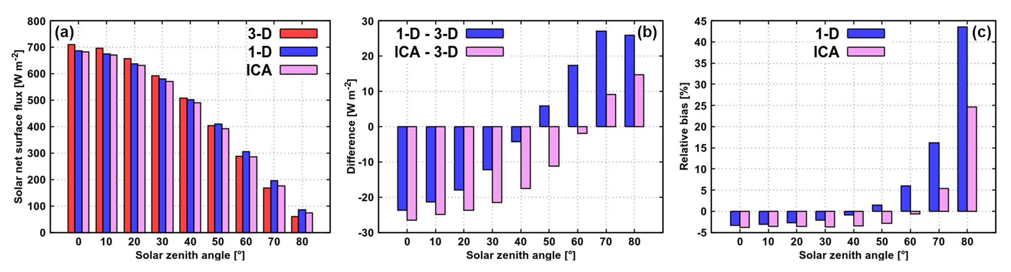
Figure 5Solar net surface flux for a cumulus cloud scene with total cloud cover of 52.3 % in the experiments with land albedo.
Motivated by the desire to understand the causes of the latter, we explore here the net surface flux in the trio (3-D, 1-D, ICA) of experiments on a single cumulus cloud scene with total cloud cover of 52.3 % over land. In the solar spectral range (Fig. 5), the net surface flux exhibits profound diurnal variation, decreasing from ∼710 W m−2 at overhead Sun to ∼60 W m−2 at SZA of 80∘ in the 3-D experiment (Fig. 5a). Similarly, the bias of the 1-D (as well as of the ICA) experiment is strongly dependent on the position of the Sun (Fig. 5b, c). At high Sun (SZA between 0 and 40∘), the 1-D experiment underestimates the 3-D benchmark, whereas at low Sun (SZA of 50∘ and larger) the opposite is the case. While the maximum absolute bias of the 1-D experiment is approximately the same for high and low Sun (about 25 W m−2), the maximum relative bias of 43 % is clearly reached at SZA of 80∘ due to strongly reduced fluxes at low Sun positions.
Again, we aim to untangle this bias dependence of 1-D experiments on SZA by first explaining purely the effects of neglected horizontal photon transport. Due to the aforementioned loss of photons through cloud sides, the diffuse downward radiation at the surface in 3-D is larger than in ICA (Wapler and Mayer, 2008). This is the main reason why solar net surface flux in the ICA experiment is underestimated relative to 3-D at Sun angles between 0 and 60∘. At SZAs larger than 60∘, however, the so-called “elongated shadow effect” (Wissmeier et al., 2013), which is generally present for all Sun positions except for overhead Sun, becomes dominant and solar net surface flux in the ICA experiment is overestimated relative to 3-D. This is essentially the cloud side illumination effect, where the effective total cloud cover (Di Giuseppe and Tompkins, 2003; Tompkins and Di Giuseppe, 2007; Hinkelman et al., 2007) increases with descending Sun, and hence also the size of the shadow increases with decreasing solar elevation, which is not taken into account in the ICA. This leads to a considerably reduced direct radiation reaching the ground and thus solar net flux in the 3-D experiment when the Sun is lower in the sky.
Both aforementioned shortcomings of ICA manifest themselves in the 1-D experiment as well. For overhead Sun, the apparent reduction of total cloud cover in the 1-D experiment due to the overlap assumption (maximal layer cloud fraction of 37.2 %, which is effectively the total cloud cover in the 1-D experiment, is appreciably lower than the total cloud cover of the 3-D cloud field, that is 52.3 %; see Fig. 3c) acts to increase the amount of direct radiation reaching the surface (compared to the 3-D or ICA case), which in turn reduces the net surface flux bias in the 1-D experiment (compared to that in the ICA experiment). When the Sun is from the side, the effective total cloud cover in the 1-D experiment remains 37.2 %, while in the 3-D experiment it is increased well beyond 52.3 %, which further increases the discrepancy in cloud shadow area at the surface in the 1-D and 3-D experiments. In particular, at SZAs larger than 60∘, both the absolute and relative biases of the 1-D experiment are by at least a factor of 2 larger than the corresponding biases of the ICA experiment.
In the thermal spectral range, the surface cools by emitting more radiation than it receives with a net flux of −62.1 W m−2 in the 3-D experiment. The emitted flux is given by the Stefan–Boltzmann law and is equal to 389.5 W m−2 (for a surface temperature of 288.2 K in the US standard atmosphere and a surface emissivity close to 1). It is by definition unbiased in the ICA and 1-D calculations. The ICA downward flux (322.6 W m−2), on the other hand, is somewhat lower than its 3-D counterpart (327.3 W m−2), because the emission of thermal radiation (at a downward angle) through cloud sides, which increases radiation at the surface, is neglected in the ICA approximation (Schäfer et al., 2016; see their Fig. 1). Due to the reduction of total cloud cover by the overlap assumption, the 1-D downward flux (316.3 W m−2) is even lower than the ICA one. This leads to the thermal net surface flux of −73.1 W m−2 in the 1-D experiment. Hence, a difference of −11.0 W m−2 between the 1-D and 3-D thermal net surface flux implies an excessive cooling of the surface during nighttime. Finally, observing the total effect during daytime, the 1-D net surface flux is found to underestimate the benchmark 3-D value at SZA between 0 and 50∘, while at larger SZAs the situation is reversed.
3.3 Dependence on surface albedo
It is well known that NWP models can have large temperature errors at coastlines (Hogan and Bozzo, 2015). Due to their high computational cost, the radiation schemes are often applied on a coarser spatial grid (compared to the grid of the NWP dynamical core). In regions along coastlines, this implies that radiative quantities computed over the ocean are being used at nearby land grid points (where surface temperature and albedo are very different), or vice versa. The alternative practice is averaging input to the radiation scheme onto the coarser grid, which has similar disadvantages.
In the previous section (Sect. 3.1 and 3.2), experiments for a solar surface albedo of 0.25 were presented. Here, we discuss how the results of these experiments change when the albedo is reduced to a typical oceanic value of 0.05, focusing on the comparison between 1-D and 3-D quantities. As albedo is thus reduced, the solar heating rate within the cloud layer in the benchmark 3-D experiments is reduced, since less radiation is reflected from the surface back towards the cloud. This reduction is largest in the lower part of the cloud layer, whereas at the height where maximum heating is reached (and above), the albedo effect is only marginal. Further, the reduction of solar heating rate with a decreased albedo is largest when the Sun is overhead, where a maximum difference of about 0.8 K d−1 is observed between 3-D heating rate profiles in the experiments with A of 0.25 and 0.05, and reduces in significance with descending Sun (at SZA of 80∘, this difference is imperceptible, essentially less than 0.05 K d−1 throughout the entire vertical extent of the cloud layer). This implies that the variation of surface albedo has a comparatively large effect on the benchmark heating rate profile at small SZAs and becomes less important with decreasing elevation of the Sun.
More relevant for this study, the difference between the 1-D and 3-D heating rate profiles in the calculations with A of 0.05 stays practically the same as in those with A of 0.25 (with a deviation being mostly less than 0.1 K d−1 at all SZAs). This means that the relative bias of the 1-D heating rate profile is generally increased as albedo is decreased. This increase of relative bias is smallest when the Sun is overhead and gains significance with descending Sun.
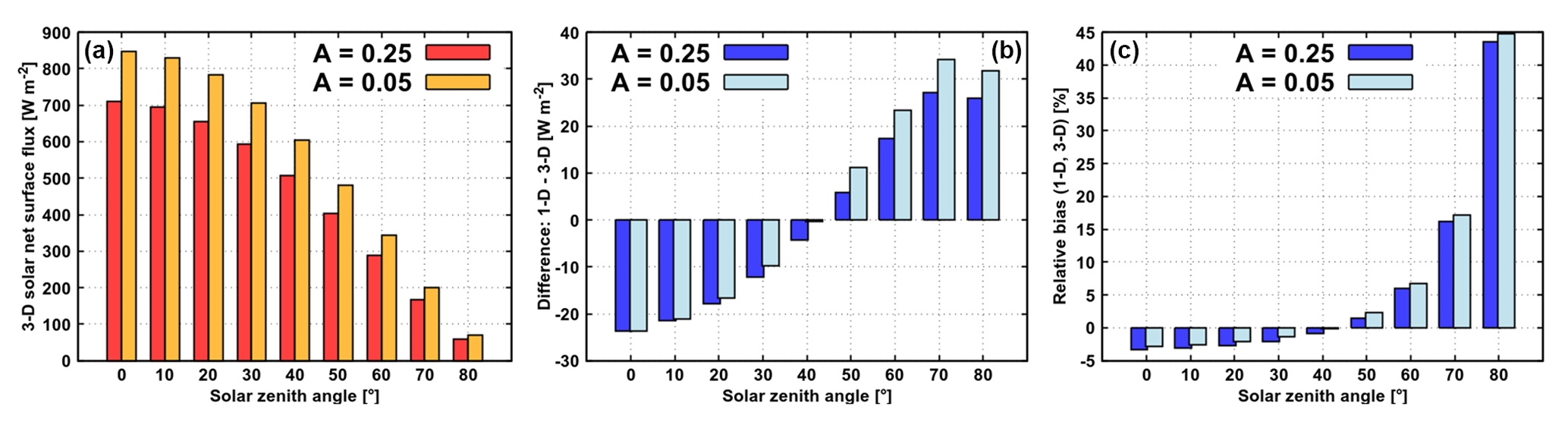
Figure 6Solar net surface flux for a cumulus cloud scene with total cloud cover of 52.3 % in the experiments with land and oceanic albedo.
Further, at the surface (Fig. 6), solar net flux in the 3-D experiment is generally increased as albedo is decreased from 0.25 to 0.05 (lower surface reflectivity implies that more radiation is absorbed in the surface). This increase is largest for overhead Sun, where the 3-D net surface flux is increased from ∼710 to ∼850 W m−2 and reduces in significance with descending Sun. The difference between the 1-D and 3-D net surface flux in the experiments with A of 0.05 stays approximately the same as in those with A of 0.25, at least at relatively high Sun (with a deviation of less than 2 W m−2 at SZA between 0 and 20∘). When the Sun is lower in the sky (SZA of 50∘ and larger), however, the overestimation of net surface flux in the 1-D experiment with A of 0.05 is enlarged (compared to the overestimation in the 1-D experiment with A of 0.25), although not more than by an additional 6 W m−2. On the whole, the relative bias of the 1-D net surface flux over the ocean stays approximately the same as over land (with a deviation of less than 2 % at all SZAs).
Referring back to the findings of Hogan and Bozzo (2015), our results regarding the sensitivity of the 3-D benchmarks on the variation of surface albedo confirm that along coastlines the radiative quantities should be computed on the regular grid (at least at higher Sun elevations). The fact that the absolute bias of cloud-layer heating rate is approximately the same over land and ocean, and that the relative bias of net surface flux over land and ocean is approximately the same as well, indicates the possibility of eliminating one parameter (namely the surface albedo) when developing a correction for NWP radiative quantities (after the robustness of the results is proved for diverse cloud scenarios).
3.4 Dependence on cloud cover
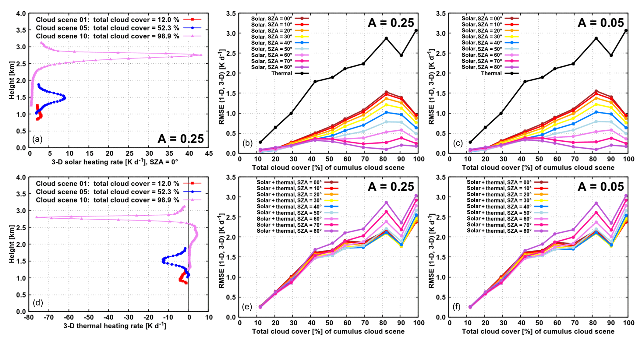
Figure 7The benchmark 3-D solar heating rate in the experiments with overhead Sun and land albedo (a) and thermal heating rate (d) in the cloud layer for the three selected cloud scenes with total cloud cover of 12.0 %, 52.3 % and 98.9 %. The RMSE between the pair (1-D, 3-D) of heating rate profiles for the entire set of 10 cumulus cloud scenes, characterized by their total cloud cover, in the experiments with land (b, e) and oceanic (c, f) albedo. Panels (a, b, c) show the RMSE in the solar and thermal spectral ranges separately, whereas (d, e, f) show the RMSE between the pair of total profiles.
We examine now the dependence of heating rates and surface fluxes on cloud cover (in addition to their dependence on SZA and albedo) by analyzing the entire data set of 10 cumulus cloud scenes. We present the benchmark 3-D experiments first and then discuss the bias of 1-D experiments (noting that the ICA experiments are investigated in Sect. 3.5, where additionally the dependence on LWP is examined). Thus, in the 3-D solar experiments over land, the heating rate within the cloud layer generally becomes larger with increasing CC of the cloud scene. At overhead Sun, for example, peak heating rates of ∼3, ∼9 and ∼43 K d−1 are seen in the experiments for cloud scenes with CCs of 12.0 %, 52.3 % and 98.9 %, respectively (Fig. 7a). The height where the peak heating is reached does not vary with SZA and is slightly above the height of maximum cloud fraction of a given cloud scene (the latter differs from scene to scene, since both the vertical extent of the cumulus cloud layer as well as the height of the maximum cloud fraction generally increase during the course of UCLA-LES simulation). Similarly, in the 3-D thermal experiments, the main cloud-radiative effects described in Sect. 3.1 (cloud top cooling, cloud side cooling, cloud base warming) in general become more pronounced as CC is increased. The peak magnitude of cooling, for example, is equal to ∼4, ∼13 and ∼76 K d−1 in the experiments for cloud scenes with CCs of 12.0 %, 52.3 % and 98.9 %, respectively (Fig. 7d). The height where this peak thermal cooling is attained at a given cloud scene corresponds well with the height of peak solar heating.
The RMSE between the pair (1-D, 3-D) of heating rate profiles in the cloud layer generally increases with CC and reaches a maximum value of 1.5 K d−1 for overhead Sun in the solar spectral range and a maximum value of 3.0 K d−1 in the thermal spectral range (Fig. 7b). Although the RMSE is a good measure of an averaged difference between the 1-D and 3-D heating rate profiles, locally the difference between 1-D and 3-D can be much larger. For the stratocumulus scene with CC of 98.9 %, for example, the cloud top cooling is overestimated by about 15 K d−1, and the cloud base warming is overestimated by about 10 K d−1 in the 1-D thermal experiment. The discrepancy between the 1-D and 3-D profiles in the thermal spectral range is quantitatively larger than in the solar spectral range and dominates the daytime RMSE at all CCs. Nevertheless, during daytime, the difference between the 1-D and 3-D solar heating rates partially compensates the corresponding thermal heating rate difference. The degree of compensation is smallest at SZA of 80∘ and increases with increasing solar elevation (Fig. 7e). The dependence of daytime RMSE on SZA is generally stronger at larger CC.
In the solar experiments over the ocean, the 3-D benchmark heating rate within the cloud layer is in general somewhat lower than that in the experiments over land, although this effect prevails at small CC and becomes less apparent at larger CC. At overhead Sun, for example, a peak heating rate is reduced by 0.5, 0.6 and 0.1 K d−1 in the experiments over the ocean (compared to the experiments over land) on cloud scenes with CCs of 12.0 %, 52.3 % and 98.9 %, respectively. This implies the relative changes of about 16.7 %, 6.7 % and 0.2 %, respectively. The RMSE between the pair (1-D, 3-D) of solar heating rate profiles in the experiments over the ocean (Fig. 7c) shows a remarkably similar dependence on SZA and CC as the RMSE in the experiments over land. The discrepancy between the RMSE values over land and ocean (at a given SZA and CC) is less than 0.1 K d−1. This suggests that the conclusions regarding the absolute bias of cloud-layer heating rate drawn in the previous section (Sect. 3.3) could be generalized to the entire set of cumulus scenes.
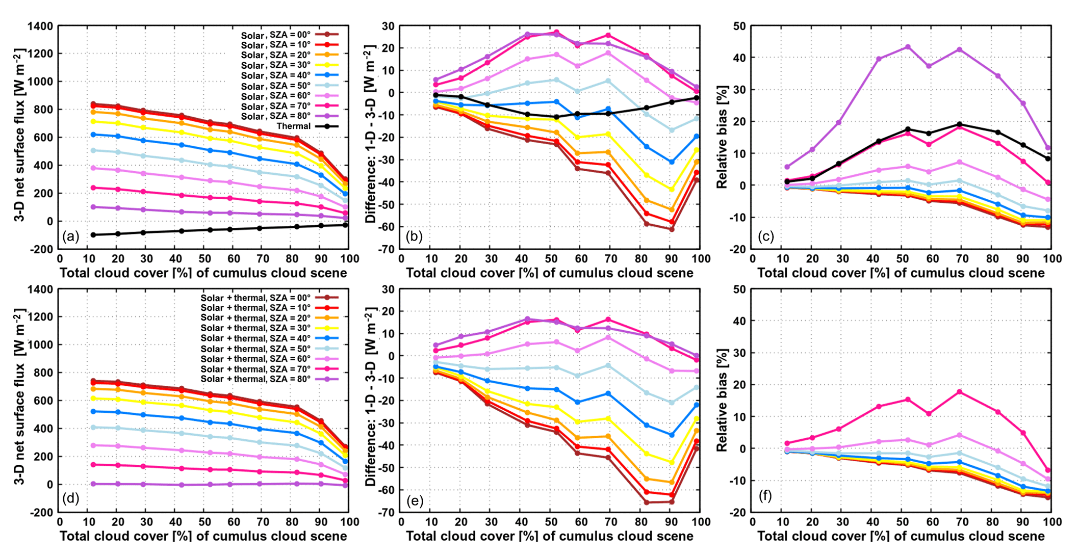
Figure 8Net surface flux for the 10 cumulus cloud scenes, characterized by their total cloud cover, in the experiments with land albedo. Panels (a, b, c) show the results in the solar and thermal spectral range separately, whereas panels (d, e, f) show the total effect of solar and thermal spectral range (large relative bias of total flux at SZA of 80∘ is off the scale and not shown on plot).
Figure 8 shows the net surface flux as a function of SZA and CC in the experiments over land. In the solar spectral range, at a given CC, the 3-D net surface flux decreases with increasing SZA, yet this decrease is stronger at smaller values of CC and reduces in significance as CC is increased. At a given SZA, on the other hand, the 3-D net surface flux gently decreases with increasing CC, up to a CC of ∼90 %, followed by a sharper drop towards considerably lower flux in the case of the fully covered scene. In the thermal spectral range, the surface cools by emitting more radiation than it receives at all CCs. While the upward emission of the surface (389.5 W m−2) is independent of CC, the downward flux at the surface increases with increasing CC. Consequently, thermal net surface flux increases with increasing CC as well. Quantitatively, the net surface flux in the solar spectral range is larger than that in the thermal spectral range, except at SZA of 80∘, where the total net surface flux is close to zero (for all values of CC). In the solar spectral range, the 1-D experiment generally overestimates the corresponding 3-D experiment at low Sun (bias up to 30 W m−2 or 45 %), while at high Sun the opposite is the case (bias up to −60 W m−2 or −10 %). This positive bias at low Sun is largest at intermediate range of CC, while negative bias at high Sun peaks at larger CC (80 % and beyond). In the thermal spectral range, the 1-D experiment overestimates the amount of 3-D cooling, with the maximal effect (−10 W m−2 or 20 %) peaked at intermediate range of CC. The daytime bias at the surface (Fig. 8e, f) is clearly governed by the solar fluxes. Nevertheless, especially at low Sun, when solar fluxes are considerably reduced, thermal fluxes play a role in modulating the surface bias as well.
In the solar experiments over the ocean (not shown), the 3-D net surface flux is generally larger than that in the experiments over land (e.g., for the cloud scene with CC of 12.0 %, a benchmark value of ∼1040 W m−2 is found at SZA of 0∘ and ∼470 W m−2 at SZA of 60∘). Interestingly, the absolute bias of the 1-D experiment over the ocean at a given SZA and CC is increased (compared to its counterpart over land) by such an amount that the relative bias of the 1-D experiment stays approximately the same as over land (with a deviation of less than 2 %), hinting that the conclusions regarding the surface bias drawn in Sect. 3.3 can be generalized to the entire set of diverse cumulus scenarios.
Finally, the reader should keep in mind that the results presented in this section should not be interpreted solely as a function of CC. With increasing CC of the scenes from the set, the cloud optical thickness increases as well. This is because both the geometrical thickness and cloud liquid water increase during the evolution of the cloud field (prior to the rain formation), which would also be expected in the real world. Further, apart from CC and LWP, there are plenty of other factors that change from scene to scene and affect the outcome of 3-D experiments and thus the bias of the 1-D calculation. These factors include 3-D cloud geometry, the number of individual clouds in the domain and their spatial distribution.
3.5 Statistical synthesis and dependence on cloud liquid water path
In order to obtain a larger data set and thus at least partially overcome the issues discussed in the last paragraph of the previous section, we slightly change the methodology that has been used so far. Namely, for each of the 10 cloud scenes, we sample a number of subscenes (“windows”), with a horizontal size of 2.8×2.8 km2 at various (x, y) coordinates within the domain. In order to create the 1-D experiment, the cloud optical properties within each window are averaged in the same manner as described in Sect. 2.4 and the two-stream method with maximum-random overlap assumption is called once per window. The 3-D and ICA experiments are then created by averaging the heating rates and surface fluxes, precalculated on highly resolved cloud fields (i.e., retaining the resolution from LES), over the same window region. Further, within each window, a total cloud cover of 3-D cloud field as well as averaged cloud liquid water path are calculated (allowing us to examine the dependence on both CC and LWP). In this way, a total of 1000 windows are analyzed for each of the three selected SZAs (0, 30 and 60∘) at each of the two surface albedos in the solar spectral range and also 1000 windows in the thermal spectral range. Figures 9 and 10 show the resulting scatter plots, where each dot represents the result of one window (note that on subfigures, where the results for the three SZAs in the solar experiments are shown simultaneously, only one-quarter of analyzed windows are displayed). It is immediately apparent that there is a strong correlation between CC and LWP. As previously suggested, this means that the findings regarding the dependencies on total cloud cover of selected cloud scenarios might be obtained similarly if the cloud scenarios were represented in terms of their optical thickness (but for the sake of brevity, we refer to this dependence solely as “CC dependence”).
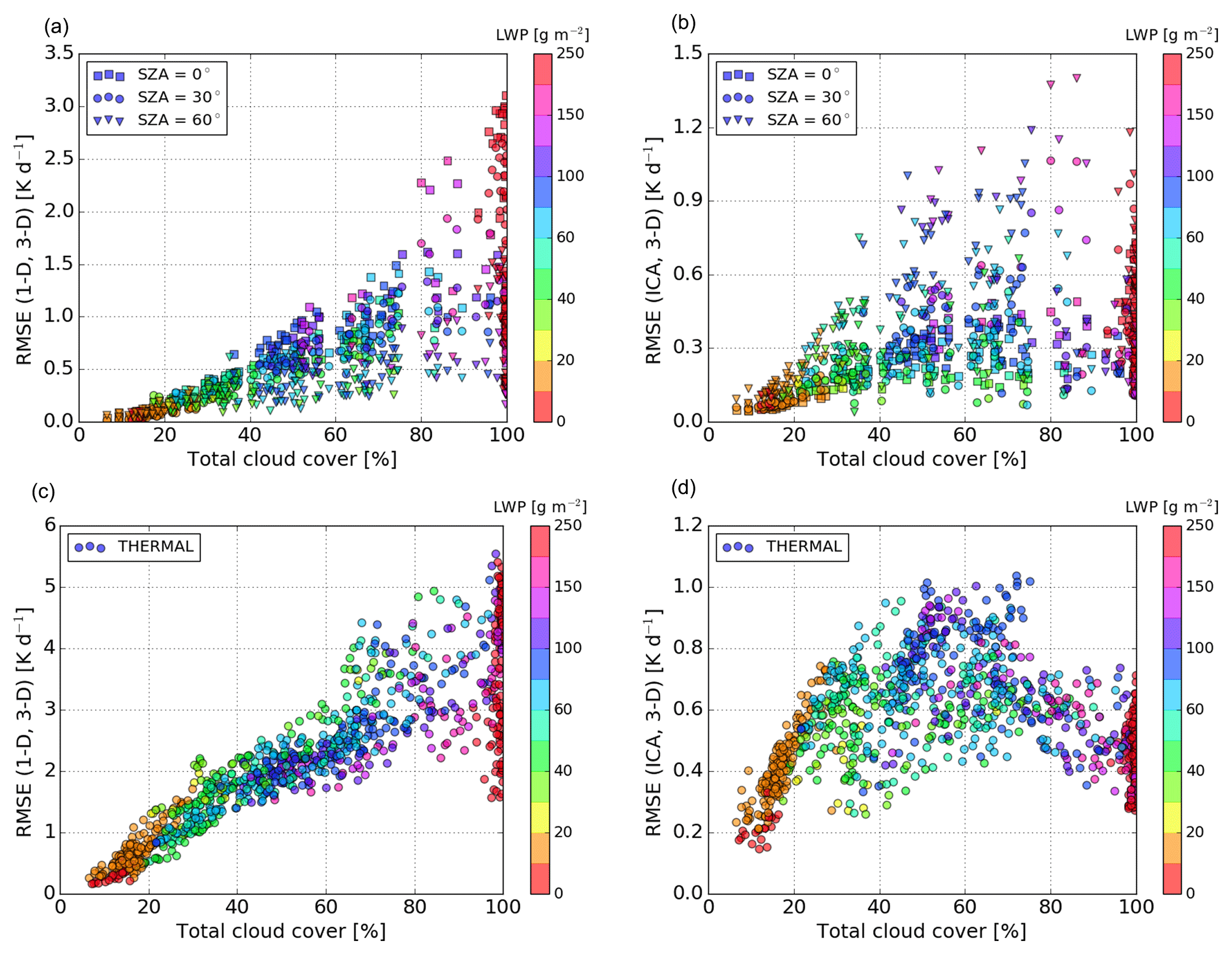
Figure 9The RMSE between the pair (1-D, 3-D) and the pair (ICA, 3-D) of solar (a, b) and thermal (c, d) heating rate profiles in the experiments with land albedo.
On the whole, the analysis of multiple windows confirms the conclusions that have been drawn in Sect. 3.4 qualitatively (regarding the bias dependence on SZA, A, CC) but extends the range of bias quantitatively. Thus, the RMSE between the pair (1-D, 3-D) of solar heating rate profiles in the experiments over land increases with CC and reaches a maximum value of ∼3.0 K d−1 for overhead Sun (Fig. 9a), which is about twice as large as the corresponding maximum based on the individual examination of the 10 cloud scenes. This suggests that the results of the case studies should be taken with caution and demonstrates the general need for statistics. The RMSE between the pair (ICA, 3-D) of solar profiles in the experiments over land (Fig. 9b) exhibits a different dependence on SZA and CC than the RMSE between the pair (1-D, 3-D). The RMSE (ICA, 3-D) peaks at intermediate CC; besides, it is smallest for overhead Sun and increases with descending Sun (cloud side illumination effect), which is the opposite of the RMSE (1-D, 3-D).
In the solar experiments over the ocean (not shown), the RMSE (1-D, 3-D) as well as the RMSE (ICA, 3-D) exhibit a qualitatively similar dependence on SZA and CC as their counterparts over land. The discrepancy between the RMSE (1-D, 3-D) over land and ocean at SZA of 0∘, for example, is less than 0.04 K d−1 in 75 % of the windows and less than 0.07 K d−1 in 95 % of the windows. Overall, this discrepancy is less than 0.1 K d−1 in all windows examined.
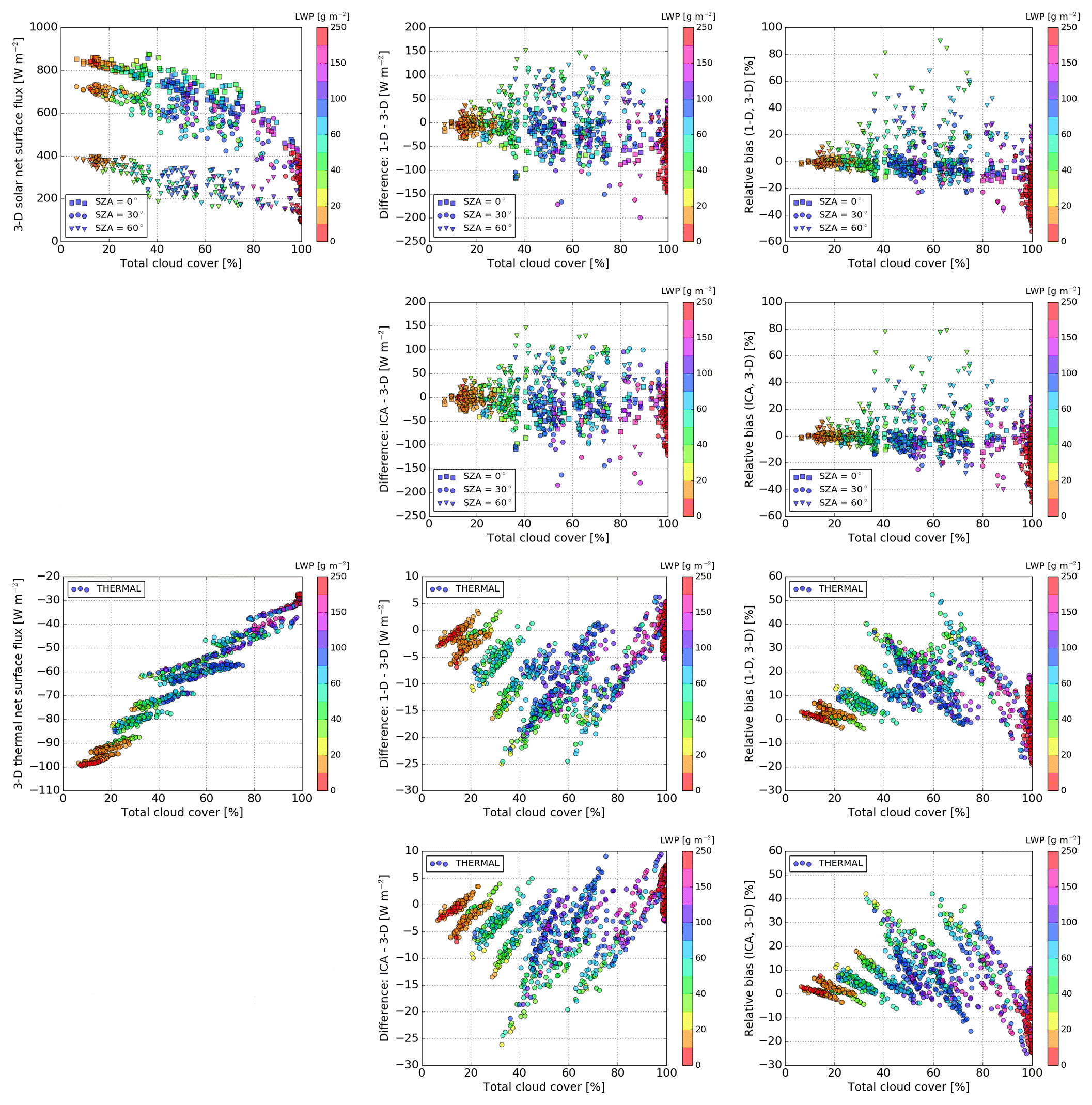
Figure 10Solar (the first and second rows) and thermal (the third and fourth rows) net surface flux in the experiments with land albedo.
The RMSE between the pair (1-D, 3-D) of thermal heating rate profiles (Fig. 9c) approximately linearly increases with CC and reaches a maximum value of ∼5.5 K d−1. The RMSE between the pair (ICA, 3-D) of thermal profiles (Fig. 9d) exhibits a significantly different dependence on CC than the RMSE between the pair (1-D, 3-D). As anticipated, the maximum RMSE (ICA, 3-D) of ∼1.0 K d−1 is reached at intermediate range of CC, where cloud side (lateral) area is maximized. This lateral surface area of clouds, namely, is the primary region subjected to strong 3-D cooling, which is neglected by the ICA. As intermediate CC is decreased (increased) towards smaller (larger) values, the cloud side area generally reduces and so does the RMSE (ICA, 3-D). At CC of 100 %, however, the RMSE (ICA, 3-D) does not fall to zero. This RMSE of about 0.5 K d−1 on average is a reminder of an important component of in-cloud horizontal photon transport between optically thicker and optically thinner regions of the cloud, leading to a discrepancy between the ICA and 3-D experiments even at overcast scenarios, where cloud side area is negligible. Furthermore, since overcast cloud scenarios are more or less maximally overlapped (see Fig. 3c), the major error source responsible for the much larger RMSE between 1-D and 3-D compared to the RMSE between ICA and 3-D of thermal profiles is attributed to the neglect of cloud horizontal heterogeneity.
To synthesize, the ICA is overall more accurate than the 1-D experiment. This suggests that the poor representation of clouds in terms of horizontal structure and vertical overlap in the 1-D experiment has a profound impact on the cloud-layer heating rate. This is especially true in the thermal spectral range and in the solar spectral range at high Sun, at intermediate and large CC, where the RMSE (1-D, 3-D) greatly surpasses the RMSE (ICA, 3-D).
Examining the dependence on LWP (at a given SZA, A, CC), we find that in the solar spectral range the RMSE (1-D, 3-D) and the RMSE (ICA, 3-D) both increase with increasing LWP. In the thermal spectral range, on the other hand, the dependence of RMSE on LWP is less straightforward, because thermal emission quickly saturates (Petters et al., 2012; see their Fig. 1).
Observing the net surface flux (Fig. 10), it is found that the 1-D solar experiment overestimates the corresponding 3-D experiment at low Sun (e.g., at SZA of 60∘, bias up to 150 W m−2 or 80 % over land and 200 W m−2 or 80 % over the ocean), while at high Sun the opposite is the case (e.g., at SZA of 30∘, bias up to −200 W m−2 or −40 % over land and −250 W m−2 or −40 % over the ocean). This positive bias at low Sun is largest at intermediate CC, while negative bias at high Sun peaks at larger CC. In the thermal spectral range, the 1-D experiment overestimates the amount of 3-D surface cooling with the maximal effect (−25 W m−2 or 50 %) peaked at intermediate CC. The bias of the ICA experiment exhibits a qualitatively similar dependence on SZA, A and CC as the bias of the 1-D experiment (in both the solar and thermal spectral ranges). Although not immediately apparent from the scatter plots, the mean ICA bias is quantitatively lower than the mean 1-D bias, which suggests that the poor representation of clouds in terms of horizontal structure and vertical overlap affects the 1-D surface bias as well.
Examining the dependence on LWP (at fixed values of other parameters), we find that the 3-D solar net surface flux decreases with increasing LWP (at least for overhead Sun). The 3-D thermal net surface flux (at a fixed CC) shows little dependence on LWP. Similarly, the dependence of surface biases on LWP is difficult to elucidate. Further investigation is needed to better quantify these effects.
The interaction between radiation and clouds represents a source of uncertainty in numerical weather prediction (NWP) due to both intrinsic problems of 1-D radiation schemes and poor representation of clouds. The underlying questions addressed in this study are how large the bias is of radiative heating rates and surface fluxes in NWP models for shallow cumulus clouds and how it scales with various input parameters of radiation schemes, such as solar zenith angle (SZA), surface albedo (A), total cloud cover (CC) and cloud liquid water path (LWP).
In order to tackle these queries, a set of radiative transfer calculations was carried out for a realistically evolving LES shallow cumulus cloud field, where cloud cover and cloud optical thickness increase with simulation time. For the study, we extracted 10 time steps with total cloud cover between ∼10 % and ∼100 %. The benchmark experiment was performed on the LES highly resolved cloud field using a 3-D Monte Carlo radiation model (abbreviated as the “3-D” experiment). In order to mimic the poor representation of shallow cumulus in NWP models, each cloud field was horizontally averaged over the cloudy part of the boxes with dimensions comparable to NWP horizontal grid spacing (several kilometers), and the common δ-Eddington two-stream method with maximum-random overlap assumption for partial cloudiness was applied (abbreviated as the “1-D” experiment). An additional experiment was conducted with the same parameter settings as 3-D, except that the Monte Carlo model was run in independent column mode (abbreviated as the “ICA” experiment). In other words, the ICA experiment preserves the LES cloud structure and only misses horizontal photon transport, whereas the 1-D experiment misrepresents real cloud structure and lacks horizontal photon transport as well. The comparison between 1-D and 3-D experiments is used to assess the overall bias of NWP radiative quantities (focus of this study), while the comparison between ICA and 3-D experiments allows to separate the effects of horizontal photon transport from those of cloud structure. Each trio (3-D, 1-D, ICA) of experiments was performed in both thermal and solar spectral ranges. In addition, SZA was varied from 0 to 80∘ with a step of 10∘, and different values of shortwave surface albedo (land, ocean) were used.
The vertical profile of the radiative heating rate directly influences atmospheric stratification. Systematic differences in cloud-layer heating rate were found between 1-D and 3-D experiments. In the solar experiments at higher Sun elevations (SZA less than 60∘, although this depends slightly on CC), as well as in the thermal experiment, the bias of the 1-D profile shows pronounced vertical gradient within the cloud layer and changes its sign approximately at the height of maximal cloud fraction. In the top part of the cloud layer (i.e., above maximal cloud fraction), the 1-D solar heating rate is too high, while in the bottom part of the cloud layer it is too low, compared to its 3-D counterpart. In the thermal spectral range, the opposite is the case, but the effect is quantitatively larger and dominates the total effect of solar and thermal spectral range (at all SZAs). Thus, during nighttime and daytime, the bias of the 1-D heating rate enhances the destabilization of the cloud layer by an overestimation of the cooling at cloud top and an overestimation of the warming at cloud bottom (a difference of about −15 K d−1 between 1-D and 3-D is observed locally for stratocumulus scenarios). Interestingly, the systematic difference between the 1-D and 3-D solar heating rate is practically insensitive to the choice of surface albedo (i.e., land versus oceanic albedo). In addition to atmospheric heating rates, net surface radiative flux has been investigated with the outcome that the 1-D solar experiment overestimates the corresponding 3-D experiment at low Sun (bias up to 80 % over land and ocean), while at high Sun the opposite is the case (bias up to −40 % over land and ocean). This positive bias at low Sun is largest at intermediate CC, while negative bias at high Sun peaks at larger CC (80 % and beyond). In the thermal spectral range, the 1-D experiment overestimates the amount of 3-D surface cooling, with the maximal bias of about 50 % peaked at intermediate CC.
Overall, the ICA experiment performs better than the 1-D experiment (with respect to the same benchmark). For the abovementioned case of stratocumulus scenarios, for example, a maximum difference of less than 1.5 K d−1 between ICA and 3-D is observed locally within the cloud layer. Therefore, one can conclude that resolving horizontally heterogeneous clouds leads to more accurate radiative heating rates than using overlapping fractional plane-parallel clouds in NWP-sized columns. Since there is a long way to go before shallow cumulus clouds will be resolved within NWP, the aforementioned conclusion implies that the current development of NWP radiation schemes should go hand in hand with the development of advanced cloud schemes generating subgrid-scale cloud structure as realistically as possible. This result is consistent with the findings of the third phase of the Intercomparison of Radiation Codes in Climate Models (ICRCCM III; Barker et al., 2003), in which ICA models outperformed the plane-parallel cloud-overlap models. The work of ICRCCM III assessing only solar radiative transfer was later extended to the thermal part of the spectrum by Kablick III et al. (2011), which brought the same conclusions. Taken together, the results of Barker et al. (2003), Kablick III et al. (2011) and the present study hint that among most promising one-dimensional radiation schemes could be the McICA algorithm (Barker et al., 2002; Pincus et al., 2003), the Tripleclouds method (Shonk and Hogan, 2008) or any other method accounting for unresolved cloud variability. The Tripleclouds method, for example, is an approach to better represent cloud horizontal inhomogeneity by using two regions in each model grid box to represent the cloud as opposed to one. One of these regions represents the optically thicker part of the cloud and the other represents the optically thinner part. The novel optimizations of the Tripleclouds method are currently being developed by the corresponding author of this paper and will be discussed in a subsequent study.
The question that needs to be addressed next is to what extent our findings for shallow water clouds apply to other cloud types. A meaningful extension of the present study would include the analogous analysis of ice clouds and mixed-phase clouds. Especially multi-layered cloud systems that form in the environment with strong vertical wind shear, where the maximum-random overlap assumption is supposed to break down, appear to be a fruitful avenue for future research. Di Giuseppe and Tompkins (2005) studied the impact of cloud cover on solar radiative biases in deep convective regimes and showed that even apparently complex 3-D convective cloud scenes can often be considered simply in terms of their quasi-two-dimensional cirrus anvil deck, which is an encouraging result.
Nevertheless, a full solution for the multiple issues of radiation schemes and their cloud-related problems in today's weather (and climate) models remains a demanding task. This is especially true at the resolution of today's regional (limited-area) numerical models, where a potential 3-D radiation parameterization should take both grid-scale and subgrid-scale radiative effects into account. This is beyond the scope of the present study but should be perceived as a stimulator for further research on radiation–cloud interactions.
The open-source UCLA-LES model is accessible at https://github.com/uclales (last access: 30 August 2018). The calculations were performed with the modified radiation interface available at Git revision “bbcc4e08ed4cc0789b33e9f2165ac63a7d0573ef”. The code for the “δ-Eddington two-stream method with maximum-random overlap assumption for partial cloudiness” will be included in the next release of libRadtran at http://www.libradtran.org (last access: 10 April 2019).
BM and NC set up the numerical experiments and developed the 1-D code together. NC carried out the experiments, evaluated the data and interpreted the results together with BM. NC prepared the manuscript with contributions from BM.
The authors declare that they have no conflict of interest.
The research leading to these results has been done within the subproject “B4: Radiative heating and cooling at cloud scale and its impact on dynamics” of the Transregional Collaborative Research Center SFB/TRR 165 “Waves to Weather” funded by the German Science Foundation (DFG). We thank Carolin Klinger and Gerard Kilroy for their perceptive comments on an earlier version of the manuscript, and Fabian Jakub for providing us with the UCLA-LES cloud field data set. Special thanks are given to Prof. George Craig for his generous support and fruitful discussion in the initial phase of this work.
This research has been supported by the Deutsche Forschungsgemeinschaft (grant no. SFB/TRR 165 Waves To Weather (W2W)).
This paper was edited by Timothy J. Dunkerton and reviewed by two anonymous referees.
Albrecht, B. A., Randall, D. A., and Nicholls, S.: Observations of marine stratocumulus clouds during FIRE, B. Am. Meteorol. Soc., 69, 618–626, https://doi.org/10.1175/1520-0477(1988)069<0618:OOMSCD>2.0.CO;2, 1988.
Albrecht, B. A., Bretherton, C. S., Johnson, D., Scubert, W. H., and Frisch, A. S.: The Atlantic stratocumulus transition experiment – ASTEX, B. Am. Meteorol. Soc., 76, 889–904, https://doi.org/10.1175/1520-0477(1995)076<0889:TASTE>2.0.CO;2, 1995.
Anderson, G. P., Clough, S. A., Kneizys, F. X., Chetwynd, J. H.m and Shettle, E. P.: AFGL Atmospheric Constituent Profiles (0–120 km). Technical Report AFGL-TR-86-0110, AFGL (OPI), Hanscom AFB, MA 01736, 1986.
Barker, H. W.: Overlap of fractional cloud for radiation calculations in GCMs: A global analysis using CloudSat and CALIPSO data, J. Geophys. Res., 113, D00A01, https://doi.org/10.1029/2007JD009677, 2008.
Baker, M. B., Austin, P. H., Blyth, A. M., and Jensen, J. B.: Small-scale variability in warm continental cumulus clouds, J. Atmos. Soc., 42, 1123–1138, https://doi.org/10.1175/1520-0469(1985)042<1123:SSVIWC>2.0.CO;2, 1985.
Barker, H. W., Pincus, R., and Morcrette, J.-J.: The Monte Carlo Independent Column Approximation: Application within large-scale models. Extended Abstracts, GCSS-ARM Workshop on the representation of cloud systems in large-scale models, Kananaskis, AB, Canada, GEWEX, 1–10, 2002.
Barker, H. W., Stephens, G. L., Partain, P. T., Bergman, J. W., Bonnel, B., Campana, K., Clothiaux, E. E., Clough, S., Cusack, S., Delamere, J., Edwards, J., Evans, K. F., Fouquart, Y., Freidenreich, S., Galin, V., Hou, Y., Kato, S., Li, J., Mlawer, E., Morcrette, J.-J., O'Hirok, W., Räisänen, P., Ramaswamy, V., Ritter, B., Rozanov, E., Schlesinger, M., Shibata, K., Sporyshev, P., Sun, Z., Wendisch, M., Wood, N., and Yang, F.: Assessing 1D Atmospheric Solar Radiative Transfer Models: Interpretation and Handling of Unresolved Clouds, J. Climate, 16, 2676–2699, https://doi.org/10.1175/1520-0442(2003)016<2676:ADASRT>2.0.CO;2, 2003.
Bugliaro, L., Zinner, T., Keil, C., Mayer, B., Hollmann, R., Reuter, M., and Thomas, W.: Validation of cloud property retrievals with simulated satellite radiances: a case study for SEVIRI, Atmos. Chem. Phys., 11, 5603–5624, https://doi.org/10.5194/acp-11-5603-2011, 2011.
Cahalan, R., Oreopoulos, L., Marshak, A., Evans, K., Davis, A., Pincus, R., Yetzer, K., Mayer, B., Davies, R., Ackerman, T. H. W. B., Clothiaux, E., Ellingson, R., Garay, M., Kassianov, E., Kinne, S., Macke, A., O’Hirok, W., Partain, P., Prigarin, S., Rublev, A., Stephens, G., Szczap, F., Takara, E., Varnai, T., Wen, G., and Zhuraleva, T.: The I3RC: Bringing together the most advanced radiative transfer tools for cloudy atmospheres, B. Am. Meteorol. Soc., 86, 1275-–1293, 2005.
Di Giuseppe, F. and Tompkins, A. M.: Effect of spatial organization on solar radiative transfer in three-dimensional idealized stratocumulus cloud fields, J. Atmos. Sci., 60, 1774–1794, https://doi.org/10.1175/1520-0469(2003)060<1774:EOSOOS>2.0.CO;2, 2003.
Di Giuseppe, F. and Tompkins, A. M.: Impact of cloud cover on solar radiative biases in deep convective regimes, J. Atmos. Sci., 62, 1989–2000, https://doi.org/10.1175/JAS3442.1, 2005.
Emde, C., Buras-Schnell, R., Kylling, A., Mayer, B., Gasteiger, J., Hamann, U., Kylling, J., Richter, B., Pause, C., Dowling, T., and Bugliaro, L.: The libRadtran software package for radiative transfer calculations (version 2.0.1), Geosci. Model Dev., 9, 1647–1672, https://doi.org/10.5194/gmd-9-1647-2016, 2016.
Fu, Q. and Liou, K. N.: On the correlated-k distribution method for radiative transfer in nonhomogeneous atmospheres, J. Atmos. Sci., 49, 2139–2156, https://doi.org/10.1175/1520-0469(1992)049<2139:OTCDMF>2.0.CO;2, 1992.
Geleyn, J. F. and Hollingsworth A.: An economical analytical method for the computation of the interaction between scattering and line absorption of radiation, Contrib. Atmos. Phys., 52, 1–16, 1979.
Hinkelman, L. M., Evans, K. F., Clothiaux, E. E., Ackerman, T. P., and Stackhouse Jr., P. W.: The effect of cumulus cloud field anisotropy on domain-averaged solar fluxes and atmospheric heating rates., J. Atmos. Sci., 64, 3499–3520, https://doi.org/10.1175/2010JCLI3752.1, 2007.
Hogan, R. J. and Bozzo, A.: Mitigating errors in surface temperature forecasts using approximate radiation updates, J. Adv. Model. Earth Syst., 7, 836–-853, https://doi.org/10.1002/2015MS000455, 2015.
Hogan, R. J. and Kew, S. F.: A 3D stochastic cloud model for investigating the radiative properties of inhomogeneous cirrus clouds, Q. J. R. Meteorol. Soc., 131, 2585–2608, https://doi.org/10.1256/qj.04.144, 2005.
Hogan, R. J. and Shonk, J. K. P.: Incorporating the effects of 3D radiative transfer in the presence of clouds into two-stream multilayer radiation schemes, J. Atmos. Sci., 70, 708–724, https://doi.org/10.1175/JAS-D-12-041.1, 2013.
Hu, Y. X. and Stamnes, K.: An accurate parameterization of the radiative properties of water clouds suitable for use in climate models, J. Climate, 6, 728–742, https://doi.org/10.1175/1520-0442(1993)006<0728:AAPOTR>2.0.CO;2, 1993.
Jakub, F. and Mayer, B.: A three-dimensional parallel radiative transfer model for atmospheric heating rates for use in cloud resolving models – The TenStream solver., J. Quant. Spectrosc. Radiat. Transfer, 163, 63–71, https://doi.org/10.1016/j.jqsrt.2015.05.003, 2015.
Jakub, F. and Mayer, B.: 3-D radiative transfer in large-eddy simulations – experiences coupling the TenStream solver to the UCLA-LES, Geosci. Model Dev., 9, 1413–1422, https://doi.org/10.5194/gmd-9-1413-2016, 2016.
Jakub, F. and Mayer, B.: The role of 1-D and 3-D radiative heating in the organization of shallow cumulus convection and the formation of cloud streets, Atmos. Chem. Phys., 17, 13317–13327, https://doi.org/10.5194/acp-17-13317-2017, 2017.
Joseph, J. H., Wiscombe, W. J., and Weinman, J. A.: The delta-Eddington approximation for radiative flux transfer, J. Atmos. Sci., 33, 2452–2459, https://doi.org/10.1175/1520-0469(1976)033<2452:TDEAFR>2.0.CO;2, 1976.
Kablick III, G. P., Ellingson, R. G., Takara, E. E., and Gu, J.: Longwave 3D benchmarks for inhomogeneous clouds and comparisons with approximate methods, J. Climate, 24, 2192–2205, https://doi.org/10.1175/2010JCLI3752.1, 2011.
Kato, S., Ackerman, T. P., Mather, J. H., and Clothiaux, E. E.: The k-distribution method and correlated-k approximation for a shortwave radiative transfer model, J. Quant. Spectrosc. Radiat. Transfer, 62, 109–121, https://doi.org/10.1016/S0022-4073(98)00075-2, 1999.
Klinger, C. and Mayer, B.: Three-dimensional Monte Carlo calculation of atmospheric thermal heating rates, J. Quant. Spectrosc. Radiat. Transfer, 144, 123–136, https://doi.org/10.1016/j.jqsrt.2014.04.009, 2014.
Klinger, C. and Mayer, B.: The neighboring column approximation (NCA) – A fast approach for the calculation of 3D thermal heating rates in cloud resolving models, J. Quant. Spectrosc. Radiat. Transfer, 168, 17–28, https://doi.org/10.1016/j.jqsrt.2015.08.020, 2016.
Klinger, C., Mayer, B., Jakub, F., Zinner, T., Park, S.-B., and Gentine, P.: Effects of 3-D thermal radiation on the development of a shallow cumulus cloud field, Atmos. Chem. Phys., 17, 5477–5500, https://doi.org/10.5194/acp-17-5477-2017, 2017.
Mayer, B.: Radiative transfer in the cloudy atmosphere, Eur. Phys. J. Confer., 1, 75–99, https://doi.org/10.1140/epjconf/e2009-00912-1, 2009.
Mayer, B. and Kylling, A.: Technical note: The libRadtran software package for radiative transfer calculations – description and examples of use, Atmos. Chem. Phys., 5, 1855–1877, https://doi.org/10.5194/acp-5-1855-2005, 2005.
Neggers, R. A. J., Duynkerke, P. G., and Rodts, S. M. A.: Shallow cumulus convection: A validation of large-eddy simulation against aircraft and Landsat observations, Q. J. R. Meteorol. Soc., 129, 2671–2696, https://doi.org/10.1256/qj.02.93, 2003.
O'Hirok, W. and Gautier, C.: A three-dimensional radiative transfer model to investigate the solar radiation within a cloudy atmosphere. Part I: Spatial effects, J. Atmos. Sci., 55, 2162–2179, https://doi.org/10.1175/1520-0469(1998)055<2162:ATDRTM>2.0.CO;2, 1998a.
O'Hirok, W. and Gautier, C.: A three-dimensional radiative transfer model to investigate the solar radiation within a cloudy atmosphere. Part II: Spectral effects, J. Atmos. Sci., 55, 3065–3076, https://doi.org/10.1175/1520-0469(1998)055<3065:ATDRTM>2.0.CO;2, 1998b.
O'Hirok, W. and Gautier, C.: The impact of model resolution on differences between Independent column approximation and Monte Carlo estimates of shortwave surface irradiance and atmospheric heating rate, J. Atmos. Sci., 62, 2939–2951, https://doi.org/10.1175/JAS3519.1, 2004.
Petters, J. L., Harrington, J. Y., and Clothiaux, E. E.: Radiative-dynamical feedbacks in low liquid water path stratiform clouds, J. Atmos. Sci., 69, 1498–1512, https://doi.org/10.1175/JAS-D-11-0169.1, 2012.
Pincus, R., Barker, H. W., and Morcrette, J.-J.: A fast, flexible, approximate technique for computing radiative transfer in inhomogeneous cloud fields, J. Geophys. Res., 108, 4376, https://doi.org/10.1029/2002JD003322, 2003.
Räisänen, P.: Two-stream approximations revisited: A new improvement and tests with GCM data, Q. J. R. Meteorol. Soc., 128, 2397–2416, https://doi.org/10.1256/qj.01.161, 2002.
Rauber, R. M., Stevens, B., Ochs III, H. T., Knight, C., Albrecht, B. A., Blyth, A. M., Fairall, C. W., Jensen, J. B., Lasher-Trapp, S. G., Mayol-Bracero, O. L., Vali, G., Anderson, J. R., Baker, B. A., Bandy, A. R., Burnet, E., Brenguier, J. L., Brewer, W. A., Brown, P. R. A., Chuang, R., Cotton, W. R., Girolamo, L. D., Geerts, B., Gerber, H., Göke, S., Gomes, L., Heikes, B. G., Hudson, J. G., Kollias, P., Lawson, R. R., Krueger, S. K., Lenschow, D. H., Nuijens, L., O'Sullivan, D. W., Rilling, R. A., Rogers, D. C., Siebesma, A. P., Snodgrass, E., Stith, J. L., Thornton, D. C., Tucker, S., Twohy, C. H., and Zuidema, P.: Rain in shallow cumulus over the ocean – The RICO campaign, B. Am. Meteorol. Soc., 88, 1912–1928, https://doi.org/10.1175/BAMS-88-12-1912, 2007.
Ritter, B. and Geleyn, J. F.: A comprehensive radiation scheme for numerical weather prediction models with potential applications in climate simulations, Mon. Wea. Rev., 120, 303–325, https://doi.org/10.1175/1520-0493(1992)120<0303:ACRSFN>2.0.CO;2, 1992.
Schäfer, S. A. K., Hogan, R., Klinger, C., Chiu, J. C., and Mayer B.: Representing 3-D cloud radiation effects in two-stream schemes: 1. Longwave considerations and effective cloud edge length, J. Geophys. Res. Atmos., 121, 8567–8582, https://doi.org/10.1002/2016JD024876.
Schmetz, J.: On the parameterization of the radiative properties of broken clouds, Tellus, 36A, 417–432, https://doi.org/10.3402/tellusa.v36i5.11644, 1984.
Schuster, A.: Radiation through a foggy atmosphere, Astrophys. J., 21, 1–22, 1905.
Schwarzschild, K.: Über das Gleichgewicht der Sonnenatmosphäre. Nachrichten von der Königlichen Gesellschaft der Wissenschaften zu Göttingen, Math.-phys. Klasse, 195, 41–53, 1906.
Shonk, J. K. P. and Hogan, R. J.: Tripleclouds: An efficient method for representing horizontal cloud inhomogeneity in 1D radiation schemes by using three regions at each height, J. Climate, 21, 2352–2370, https://doi.org/10.1175/2007JCLI1940.1, 2008.
Stephens, G. L. and Webster, P. J.: Clouds and climate: Sensitivity of simple systems, J. Atmos. Sci., 38, 235–247, https://doi.org/10.1175/1520-0469(1981)038<0235:CACSOS>2.0.CO;2, 1981.
Stephens, G. L., Gabriel, P. M., and Partain, P. T.: Parameterization of atmospheric radiative transfer. Part I: Validity of simple models,J. Atmos. Sci., 58, 3391–3409, https://doi.org/10.1175/1520-0469(2001)058<3391:POARTP>2.0.CO;2, 2001.
Tiedtke, M.: A comprehensive mass flux scheme for cumulus parameterization in large-scale models, Mon. Wea. Rev., 117, 1779–1800, https://doi.org/10.1175/1520-0493(1989)117<1779:ACMFSF>2.0.CO;2, 1989.
Tompkins, A. M. and Di Giuseppe, F.: Generalizing cloud overlap treatment to include solar zenith angle effects on cloud geometry, J. Atmos. Sci., 64, 2116–2125, https://doi.org/10.1175/JAS3925.1, 2007.
Wapler, K. and Mayer, B.: A fast three-dimensional approximation for the calculation of surface irradiance in large-eddy simulation models, J. Appl. Meteor. Climatol., 47, 3061–3071, https://doi.org/10.1175/2008JAMC1842.1, 2008.
Wissmeier, U., Buras, R., and Mayer, B.: paNTICA: A fast 3D radiative transfer scheme to calculate surface solar irradiance for NWP and LES models, J. Appl. Meteor. Climatol., 52, 1698–1715, https://doi.org/10.1175/JAMC-D-12-0227.1, 2013.
Wu, X. and Liang, X. Z.: Radiative effects of cloud horizontal inhomogeneity and vertical overlap identified from a monthlong cloud-resolving model simulation, J. Atmos. Sci., 62, 4105–4112, https://doi.org/10.1175/JAS3565.1, 2005.
Zhao, M. and Austin, P. H.: Life cycle of numerically simulated shallow cumulus clouds. Part I. Transport, J. Atmos. Sci., 62, 1269–1290, https://doi.org/10.1175/JAS3414.1, 2005.
Zdunkowski, W., Trautmann, T., and Bott, A.: Radiation in the atmosphere – A course in theoretical meteorology, Cambridge University Press, New York, 2007.
We follow the convention of i, j increasing downward from the top of the atmosphere, where i=0, j=1. Index i is used for level variables, whereas index j is used for layer variables. The N vertical layers, which are enumerated from 1 to N, are enclosed by (N+1) vertical levels, which are enumerated from 0 to N.
This can be partially justified by the fact that NWP models have relatively fine vertical grid spacing in the planetary boundary layer, although we agree that proper handling of variable vertical resolution would deserve further attention. Hogan and Kew (2005) investigated radiative quantities that would be diagnosed by a general circulation model (GCM) and represented the cloud with the vertical resolution of 60 m, which is much better than the resolution of current GCMs. They stated, however, that when the vertical resolution is degraded by a factor of 4, the fluxes are the same to within 0.5 W m−2 in the shortwave and 0.2 W m−2 in the longwave.