Modelling CO₂ weather – why horizontal resolution matters

Climate change mitigation efforts require information on the current greenhouse gas atmospheric concentrations and their sources and sinks. Carbon dioxide (CO₂) is the most abundant anthropogenic greenhouse gas. Its variability in the atmosphere is modulated by the synergy between weather and CO₂ surface fluxes, often referred to as CO₂ weather. It is interpreted with the help of global or regional numerical transport models, with horizontal resolutions ranging from a few hundreds of kilometres to a few kilometres. Changes in the model horizontal resolution affect not only atmospheric transport but also the representation of topography and surface CO₂ fluxes. This paper assesses the impact of horizontal resolution on the simulated atmospheric CO₂ variability with a numerical weather prediction model. The simulations are performed using the Copernicus Atmosphere Monitoring Service (CAMS) CO₂ forecasting system at different resolutions from 9 to 80 km and are evaluated using in situ atmospheric surface measurements and atmospheric column-mean observations of CO₂, as well as radiosonde and SYNOP observations of the winds.

The results indicate that both diurnal and day-to-day variability of atmospheric CO₂ are generally better represented at high resolution, as shown by a reduction in the errors in simulated wind and CO₂. Mountain stations display the largest improvements at high resolution as they directly benefit from the more realistic orography. In addition, the CO₂ spatial gradients are generally improved with increasing resolution for both stations near the surface and those observing the total column, as the overall inter-station error is also reduced in magnitude. However, close to emission hotspots, the high resolution can also lead to a deterioration of the simulation skill, highlighting uncertainties in the high-resolution fluxes that are more diffuse at lower resolutions.

We conclude that increasing horizontal resolution matters for modelling CO₂ weather because it has the potential to bring together improvements in the surface representation of both winds and CO₂ fluxes, as well as an expected reduction in numerical errors of transport. Modelling applications like atmospheric inversion systems to estimate surface fluxes will only be able to benefit fully from upgrades in horizontal resolution if the topography, winds and prior flux distribution are also upgraded accordingly. It is clear from the results that an additional increase in resolution might reduce errors even further. However, the horizontal resolution sensitivity tests indicate that the change in the CO₂ and wind modelling error with resolution is not linear, making it difficult to quantify the improvement beyond the tested resolutions.

Finally, we show that the high-resolution simulations are useful for the assessment of the small-scale variability of CO₂ which cannot be represented in coarser-resolution models. These representativeness errors need to be considered when assimilating in situ data and high-resolution satellite data such as Greenhouse gases Observing Satellite (GOSAT), Orbiting Carbon Observatory-2 (OCO-2), the Chinese Carbon Dioxide Observation Satellite Mission (TanSat) and future missions such as the Geostationary Carbon Observatory (GeoCarb) and the Sentinel satellite constellation for CO₂. For these reasons, the high-resolution CO₂ simulations provided by the CAMS in real time can be useful to estimate such small-scale variability in real time, as well as providing boundary conditions for regional modelling studies and supporting field experiments.

1 Introduction

Over synoptic weather timescales of hours to days and spatial scales less than 1000 km, the assumption that atmospheric CO₂ is well-mixed into a homogeneous background does not hold, as shown by the observed variability at baseline in situ stations (e.g. Halter and Harris, 1983). CO₂ weather is defined here as the atmospheric CO₂ variability at timescales and spatial scales of weather systems (Parazoo et al., 2011) as depicted in Fig. 1. It reflects a complex combination of anthropogenic and natural CO₂ fluxes near the Earth's surface and transport by weather systems in the atmosphere (Geels et al., 2004; Patra et al., 2008). This synergy of CO₂ fluxes and weather results in intricate atmospheric CO₂ patterns of positive and negative anomalies, collocated with weather variations on top of the well-mixed CO₂ background that varies slowly on timescales of weeks to years (Keeling et al., 1976).

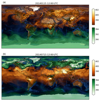
Figure 1 Snapshots of column-averaged CO₂ (XCO₂) (ppm) above (in reds) and below (in greens) the global mean on 15 January (a) and 15 July (b) at 12:00 UTC from the Copernicus Atmosphere Monitoring Service global CO₂ forecast at high horizontal resolution (∼9 km).

Modelling the synoptic-scale transport that modulates the CO₂ weather is crucial for interpreting the variability of surface CO₂ concentrations from in situ observations (Law et al., 2010) and column-averaged CO₂ from satellite and ground-based observations (Corbin et al., 2008) and for forecasting CO₂ from 1 to 10 d ahead (Agustí-Panareda et al., 2014; Tang et al., 2018) in order to examine the predictive skill of the models. Tracer transport models use the numerical schemes and meteorological information of numerical weather prediction (NWP) to simulate the tracer variability in the atmosphere. Increasing the horizontal resolution associated with the grid spacing of tracer transport models has the benefit of reducing the numerical errors in tracer simulations, leading to convergence of the transport solution from different transport schemes (Prather et al., 2008). NWP models for weather forecasting have been doubling the global horizontal resolution approximately every 8 years (Wedi, 2014) in order to improve the forecast skill. But until now, global tracer transport models have generally used lower resolution than NWP models, as chemical transport models including chemistry and/or long window data assimilation cannot afford such computational expense.

Observations of atmospheric CO₂ are used in data assimilation systems based on tracer transport models to produce optimal estimates of atmospheric CO₂ concentrations (e.g. Massart et al., 2016) or model parameters and CO₂ fluxes in atmospheric inversion systems (e.g. Rayner et al., 2005; Chevallier et al., 2010). If tracer transport models cannot represent the synoptic variability accurately, then the resulting errors when comparing the tracer from the model with observations will prevent these observations from being used effectively in the data assimilation systems (e.g. Brooks et al., 2012). The model–observation mismatch caused by differences in the resolution of the tracer transport model – including both the resolution of the meteorological fields and the resolution of the fluxes on the model grid – and the resolution of the observation footprint is also known as representativeness error. Failure to properly account for representativeness errors in data assimilation will lead to errors in the optimised parameters, whether atmospheric concentrations, model parameters or surface fluxes.

Several studies have investigated the spatial representativeness errors of CO₂ (Miller et al., 2007; van der Molen and Dolman, 2007; Corbin et al., 2008; Tolk et al., 2008) by analysing the CO₂ distribution within model grid cells, based on nested high-resolution simulations on limited domains over Europe, North America and South America for certain months or by statistical parameterisation of CO₂ covariances based on lower-resolution simulations (Alkhaled et al., 2008). The importance of high resolution over complex terrain has also been demonstrated on regional scales, e.g. in Europe (van der Molen and Dolman, 2007; Ahmadov et al., 2009; Pillai et al., 2011) and in North America (Lin et al., 2017; Hedelius et al., 2017) using very high resolution simulations (down to 1 km). However, other studies with coarser global tracer transport models have compared CO₂ simulations with a range of resolutions from a few degrees down to 0.5^∘ without finding significant improvements with respect to observations (Lin et al., 2018; Remaud et al., 2018).

The full impact of horizontal resolution on the simulated tracer variability depends on the resolution of transport and emissions/biogenic fluxes (e.g. Vogel et al., 2013) as well as the resolution of the topography and the winds (e.g. Sekiyama et al., 2015) in the model. In this study the full sensitivity of CO₂ synoptic variability to the model horizonal resolution (including all the aspects mentioned above) is investigated by quantifying the change in model error with horizontal resolution at observing stations. Three main questions are addressed:

1. What is the sensitivity of the modelled atmospheric CO₂ variability at diurnal and synoptic timescales to horizonal resolution?

2. How is horizontal resolution affecting the medium-range (1–10 d) forecast error growth of atmospheric CO₂?

3. What are the typical CO₂ representativeness errors in models with horizontal resolutions of 1^∘ × 1^∘, currently considered as high resolution in tracer transport models, and where and when are these representativeness errors largest?

The model simulations use the operational Copernicus Atmosphere Monitoring Service (CAMS) global CO₂ forecasting system (Agustí-Panareda et al., 2014; Massart et al., 2016) which is based on the Integrated Forecasting System (IFS) model of the European Centre for Medium-Range Weather Forecasts (ECMWF). They are performed over a range of resolutions currently used operationally in NWP from 9 to 80 km. A detailed description of the simulations, observations and tools used to assess the importance of horizontal resolution for simulating atmospheric CO₂ variability related to weather is presented in Sect. 2. Section 3 shows the impact of horizontal resolution on the error of simulated horizontal winds (Sect. 3.1) and atmospheric CO₂ (Sect. 3.2 and 3.3). The results of the sensitivity to horizontal resolution are explained in the context of the small-scale variability in Sect. 3.4. The diagnostics of small-scale variability provide an estimate of the expected representativeness errors for CO₂ simulations with coarser horizontal resolutions. Finally, an example of an urban site is shown in Sect. 3.5, where the impact of horizontal resolution is positive in January and negative in July. The implications of the results for CO₂ forecasting and atmospheric inversion systems are discussed in Sect. 4, with a summary of the main findings on why and where horizontal resolution matters.

2 Methodology

2.1 Observations

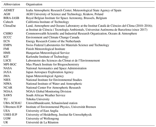
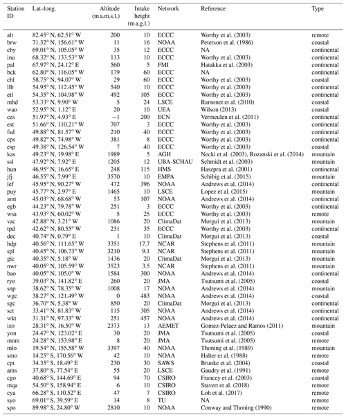
Continuous in situ observations near the surface and column-averaged observations from the Total Carbon Column Observing Network (TCCON) provide the reference for atmospheric CO₂ variability. Figure 2 shows the spatial distribution of the CO₂ observing stations used in this study. Hourly near-surface CO₂ observations are provided by 51 in situ stations operated by various organisations throughout the period of the simulations: data from 44 stations are taken from the cooperative GLOBALVIEWplus (ObsPack , 2015) data set, and additional data have been obtained from three additional stations from CSIRO in Australia and Antarctica and four stations from the ClimaDat network (Morguí et al., 2013, 2017) over the Iberian Peninsula. The cooperative GLOBALVIEWplus (ObsPack , 2015) data set is coordinated by NOAA, and it comprises data collected by various institutions and laboratories including AEMET, AGH, CSIRO, ECCC, ECN, EMPA,FMI, HMS, LSCE, NCAR, NOAA, JMA, NIWA, SAWS, TU, UBA-SCHAU, UEA, UHEI-IUP and UR (see Tables A1 and A2 for full list of stations with their organisations and associated references). No selection criteria are applied to the stations from the GLOBALVIEWplus ObsPack  (2015), CSIRO and ClimaDat data sets, other than availability of hourly data for January and July 2014.

Figure 2 Map of in situ (blue squares) and TCCON (red triangles) stations. Detailed information on each station is provided in Tables A1 and A3.

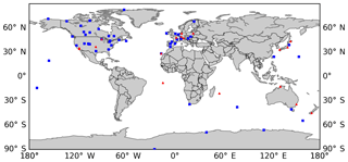
Most stations are on the World Meteorological Organization (WMO) CO₂ scale, although the inter-calibration of standard gases is not critical for this study because the focus is on the relative difference between the high- and low-resolution simulations to quantify the sensitivity of modelled CO₂ to horizontal resolution in the model. The distribution of the stations is not homogeneous over the globe. However, there is a wide variety of locations that sample synoptic variability on various types of terrain including many coastal, mountain, continental and oceanic sites over different continents on both hemispheres. Wind observations from around 400 radiosondes stations and all the operational 10 m SYNOP stations around the globe are used to evaluate the sensitivity of wind errors to the model horizontal resolution at different atmospheric levels in the troposphere.

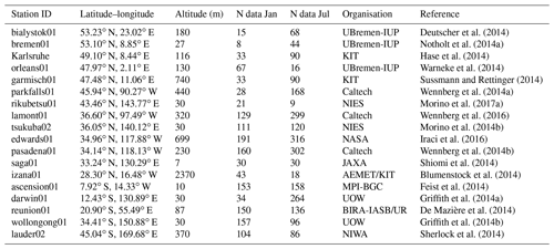
Total column observations from 18 TCCON Fourier transform spectrometers (FTSs) (Wunch et al., 2011) available in January and July 2014 – shown as red triangles in Fig. 2 – are also used to evaluate the variability of the column-averaged dry-air mole fraction of CO₂ – hereafter referred to as XCO₂ – (Table A3). These TCCON observations are retrieved from direct solar near-infrared spectra (http://www.tccon.caltech.edu, last access: 30 May 2019), and they provide a ground reference to the GOSAT (Kuze et al., 2009), OCO-2 (Crisp et al., 2017) and TanSat (Yang et al., 2018) satellite observations (e.g. Inoue et al., 2016; Wunch et al., 2017). Total column averages are less sensitive to the uncertainties associated with vertical mixing than the CO₂ abundances near the surface. However, the temporal coverage of TCCON observations is limited to clear-sky and sunny conditions, which means there are generally more gaps in the TCCON data than in near-surface in situ data.

2.2 Global atmospheric CO₂ model

The model used in this study is the Integrated Forecasting System (IFS), the same model used in NWP at ECMWF and in the CAMS atmospheric composition analysis and forecasting system to issue 5 d CO₂ and CH₄ forecasts (https://atmosphere.copernicus.eu/charts/cams/carbon-dioxide-forecasts, last access: 30 May 2019), as well as reactive gases and aerosol forecasts relevant for air quality (Flemming et al., 2015; Morcrette et al., 2009). The IFS model version is CY43r1, the operational weather forecast model at ECMWF from 22 November 2016 to 10 July 2017. A full evaluation of this model cycle can be found in Haiden et al. (2017). The high horizontal resolution is based on a cubic octahedral reduced Gaussian – called hereafter octahedral – grid (Holm et al., 2016). The implementation of the octahedral grid has allowed a substantial increase in the grid point resolution from 16 km to approximately 9 km, without having to increase the spectral resolution of the model (Malardel et al., 2016). The 9kmEXP simulation comprises up to 904 million model grid points, 137 levels and a time step of 7.5 min.

The tracer transport is modelled by three different numerical schemes to represent (i) the resolved advection of CO₂ by the winds, and the sub-grid-scale (ii) convection and (iii) turbulent mixing processes that need to be parameterised. The tracer advection is computed using a semi-implicit semi-Lagrangian scheme (Temperton et al., 2001; Diamantakis and Magnusson, 2016) which is an unconditionally stable method for the integration of the transport equations and for the fast terms associated with gravity waves. Semi-Lagrangian advection schemes have small dispersion and phase speed errors despite using long time steps (Staniforth and Côté, 1991). In practice, these properties mean that the time step is limited only by the local truncation error and not by numerical stability bounds. The semi-Lagrangian advection scheme in the IFS is not mass-conserving. Thus, a mass fixer is required to ensure mass conservation at every time step (Agustí-Panareda et al., 2017; Diamantakis and Agustí-Panareda, 2017). The turbulent mixing scheme is described in Beljaars and Viterbo (1998), Koehler et al. (2011) and Sandu et al. (2013). The convection scheme is based on Tiedtke (1989) (see Bechtold et al., 2008, 2014, for further details). Full documentation of the IFS can be found at https://www.ecmwf.int/en/forecasts/documentation-and-support/changes-ecmwf-model/ifs-documentation (last access: 30 May 2019).

The CO₂ surface fluxes from the ocean, biomass burning and anthropogenic emissions are prescribed using inventories or climatologies, while the biogenic fluxes over land are modelled online (see Table 1). The anthropogenic CO₂ emissions come from the EDGAR v4.2 FT2010 inventory for 2012 (last year with gridded emissions). They are extrapolated in time to the year of the simulation with country trends provided by the EDGAR database (http://edgar.jrc.ec.europa.eu, last access: 30 May 2019). The biogenic CO₂ emissions from land vegetation are modelled with the A-gs photosynthesis scheme and an empirical model to simulate the ecosystem respiration fluxes which are integrated in the CHTESSEL land surface model of the IFS (Boussetta et al., 2013). The fluxes have been evaluated with FLUXNET data and compared to different models (e.g. CASA and ORCHIDEE) showing a comparable performance on synoptic to seasonal scales (Balzarolo et al., 2014). An online bias correction scheme (Agustí-Panareda et al., 2016) is applied to the modelled gross primary production (GPP) and ecosystem respiration (Reco) fluxes to correct for biases in the net ecosystem exchange (NEE) budget on a timescale of 10 d compared to a climatology of optimised fluxes (Chevallier et al., 2010). Figure S1 in the Supplement shows the monthly mean NEE for the highest and lowest resolutions.

Olivier and Janssens-Maenhout (2015)Kaiser et al. (2012)Takahashi et al. (2009)Boussetta et al. (2013)Agustí-Panareda et al. (2016)

Table 1 Datasets and models of CO₂ fluxes used in simulations listed in Table 2.

The atmospheric tracer transport and CO₂ biogenic fluxes are two of the largest contributors to the synoptic variability of atmospheric CO₂ globally (Geels et al., 2004; Agustí-Panareda et al., 2014). Thus, the modelling of these two components online in the IFS allows us to investigate the full impact of the resolution coming from the winds and the tracer transport, as well as the fluxes.

2.3 Global atmospheric CO₂ simulations

A set of global simulations are performed at several resolutions from 9 to 80 km (Table 2) to investigate the impact of horizontal resolution on the modelled CO₂ variability at diurnal and synoptic scales. These are the resolutions that are currently used operationally in global meteorological reanalysis – e.g. ERA-Interim at 80 km (Dee et al., 2011) – widely used in tracer transport models and the typically higher resolutions of operational weather forecasts models. For instance, the deterministic weather forecast at ECMWF currently runs at 9 km resolution, and it was the global forecasting system with the highest resolution in the world when it was introduced on 8 March 2016 (Holm et al., 2016).

Table 2 List of simulations with different resolutions given by different model grids. All simulations use 137 vertical model levels. All the experiments have been performed in January and July 2014 using the same CO₂ surface fluxes (see Table 1).

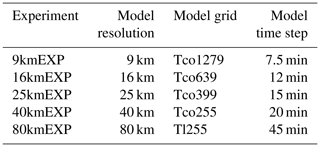
The octahedral grid is used for all simulations, except for the lowest-resolution simulation at 80 km which uses a reduced linear Gaussian grid as in the ERA-Interim and CAMS Reanalysis (Inness et al., 2019). The time steps are also dependent on the horizontal resolution and range from 7.5 to 45 min. As described in Sect. 2.2, the semi-implicit semi-Lagrangian method used in the IFS is free from stability restrictions. Thus, the model uses the longest possible time step that provides the most accurate result for each spatial resolution. This is selected through experimentation and validation, but a rule of thumb is that as the horizontal resolution increases, the time step decreases to keep the mean Courant–Friedrichs–Lewy (CFL) number constant. This typically leads to much longer time steps than Eulerian models for which their time step is restricted by the typical CFL stability limit (i.e. the maximum CFL number being less than 1).

All the simulation experiments are conducted for a winter and a summer month, in January and July 2014, as we expect that winter and summer periods will show markedly different variability patterns in CO₂. Figure 3 shows the configuration of the simulations. A 10 d forecast is performed at 00:00 UTC each day of the month. The meteorological initial conditions of each forecast come from the ECMWF operational NWP analysis (Rabier et al., 2000), whereas the atmospheric CO₂ tracer is initialised with the previous 1 d forecast, which means CO₂ is essentially free-running, as in Agustí-Panareda et al. (2014). The first initial conditions for CO₂ on 1 January and 1 July 2014 are extracted from the CAMS CO₂ analysis (Massart et al., 2016). NWP analysis of meteorological fields is one of the main elements determining the quality of the tracer transport (Locatelli et al., 2013; Polavarapu et al., 2016). Keeping the meteorological fields close to the analysis by having a sequence of 1 d forecasts ensures the tracer transport is as realistic as possible. Therefore, the sequence of 1 d forecasts is used as the standard (cyclic forecast) configuration for the simulations at different resolutions.

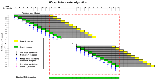
Figure 3 Schematic of CO₂ simulations with cyclic forecast configuration with 10 d forecasts initialised every day from 1st of the month to the 10th day of the following month. Initial conditions are depicted by arrows (see legend), and the period of evaluation in which several forecast lead times can be compared is delimited by the red dashed line. The standard CO₂ simulations are composed by a series of 1 d forecasts as shown by the green rectangles.

The extension to the 10 d forecasts allows us to assess the impact of errors in the meteorological fields – which grow during the forecast – on the CO₂ simulations. There are 10 realisations of CO₂ for each day, one for each forecast lead time (Fig. 3). Each forecast lead time is evaluated separately in order to estimate the error growth during the forecast. For consistency in the evaluation of the different forecast lead times, the periods from 10 January to 10 February and 10 July to 10 August are used in the validation diagnostics.

The simulations also include an additional CO₂ tracer which is only transported (i.e. does not respond to CO₂ surface fluxes) during the forecast. We refer to this tracer as NFX. This tracer is still initialised with the standard CO₂ at the beginning of each forecast. The difference between the NFX CO₂ and the standard CO₂ tracers can provide insight into the sensitivity to local flux at different horizontal resolutions. Similarly, the change in the error of the simulation with resolution for both the standard and the NFX tracers can be used as an indicator of transport versus local flux influence in the assessment of the impact of horizontal resolution.

2.4 Diagnostics for model evaluation

The focus of this paper is on assessing the skill of the model in simulating CO₂ weather with short-term variability over a period of a month. For this purpose, the root mean square error

$$\begin{array}{}\text{(1)}& \mathrm{RMSE}=\sqrt{{\displaystyle \frac{\mathrm{1}}{N}}\sum _{i=\mathrm{1}}^N(m_i-o_i{)}^{\mathrm{2}}},\end{array}$$

the systematic error or bias

$$\begin{array}{}\text{(2)}& \mathit{\mu }={\displaystyle \frac{\mathrm{1}}{N}}\sum _{i=\mathrm{1}}^N(m_i-o_i)\end{array}$$

and the random error

$$\begin{array}{}\text{(3)}& \mathrm{STDE}=\sqrt{{\displaystyle \frac{\mathrm{1}}{N}}\sum _{i=\mathrm{1}}^N(m_i-o_i-\mathit{\mu }{)}^{\mathrm{2}}}\end{array}$$

of the modelled CO₂ dry molar fraction (m) are computed with respect to N hourly observations (o) at each observing site. The standard deviation of the site error – also known as inter-station error – is used as an indicator of the spatial variability of the error e (e.g. RMSE, μ) between the M observing sites:

$$\begin{array}{}\text{(4)}& {\mathit{\sigma }}_e=\sqrt{{\displaystyle \frac{\mathrm{1}}{M-\mathrm{1}}}\sum _{s=\mathrm{1}}^M(e_s-\stackrel{\mathrm{‾}}{e}{)}^{\mathrm{2}}},\end{array}$$

where $\stackrel{\mathrm{‾}}{e}$ is the mean error of all sites. It reflects the skill of the model in representing spatial gradients between the sites. The Pearson’s correlation coefficient is also used to assess the skill of the model in simulating the diurnal and synoptic variability at the sites.

The model is sampled in the horizontal by taking the nearest grid point to the station over land. This approach is widely used in model evaluation (Patra et al., 2008) as it allows assessment of the model directly at grid point scale. At coastal locations, coarse-resolution models can find a better fit to observations by sampling the nearest ocean grid point as land grid points tend to overestimate the diurnal cycle (Law et al., 2010). For this reason, the sampling protocol for observations in the atmospheric inversion system moves some stations offshore (Gurney et al., 2003). However, coastal sites can be influenced by both ocean and land, which means that they will have contrasting periods sampling baseline air associated with low variability and periods with land and local influences associated with high CO₂ variability (Patra et al., 2008). In this study we have chosen to consistently sample the nearest land point over land because we are interested in assessing the capabilities of the model to represent both baseline and local influences. The temporal sampling is performed with a linear interpolation from the 3-hourly archived model fields to the observation time as in Agustí-Panareda et al. (2014).

At the surface stations, the model is also interpolated to the altitude of the sampling height above ground level (a.g.l.). This ensures the same model levels are used for the different horizontal resolutions. The model has hybrid coordinates that follow the terrain close to the surface. Selecting the model level at the station height above mean sea level (a.m.s.l.) would imply the use of different model levels for different resolutions when the orographic height varies between the horizontal resolutions. It would therefore lead to comparisons of CO₂ in the planetary boundary layer and free troposphere at mountain sites where the low-resolution model underestimates the orographic height. Lin et al. (2017) tested both approaches at several mountain sites. They found that the sampling at a.m.s.l. greatly underestimates the amplitude of the diurnal cycle, as the sensitivity to local fluxes is reduced at higher levels above the ground. Since most low-resolution models used in atmospheric inversions tend to use the model sampling a.m.s.l. at mountain sites (e.g. Wang et al., 2018), a comparison of the two approaches (a.g.l. and a.m.s.l.) is provided in the Supplement. At the TCCON stations, the model profile is processed with the TCCON averaging kernel and prior, as described in Appendix A of Massart et al. (2016).

Atmospheric CO₂ variability is subject to local- or small-scale influences (<100 km) associated with complex topography, coastal boundaries, local fluxes and mesoscale atmospheric flow (Lin, 2007). Most models used in carbon cycle studies are unable to represent such local variability. The resulting representativeness errors reflect the sub-grid-scale variability associated with the coarse resolution of the models (e.g. Tolk et al., 2008). At high resolution it is possible to estimate part of this sub-grid-scale variability of coarser models. In order to do that, the 9kmEXP simulation is interpolated onto a 0.1^∘ × 0.1^∘ regular lat–long. grid, and subsequently it is sampled for each time zone (computed hourly along longitude) at 13:00 ± 0.5 h local time. This temporal sampling at 13:00 is consistent with the GOSAT (http://www.gosat.nies.go.jp/en/, last access: 30 May 2019) and OCO-2 (http://oco.jpl.nasa.gov/mission, last access: 30 May 2019) overpass time. Thus, it provides a more relevant estimate of the potential representativeness error for lower-resolution inversion systems, which use daytime surface in situ data and satellite data (e.g. Chevallier et al., 2010, 2014). The representativeness error is estimated by computing the standard deviation of the CO₂ dry molar fraction at 0.1^∘ resolution within the coarser grid boxes of 1^∘ × 1^∘ over the whole globe:

$$\begin{array}{}\text{(5)}& {\mathit{\sigma }}_{{\mathrm{CO}}_{\mathrm{2}}}=\sqrt{{\displaystyle \frac{\mathrm{1}}{n-\mathrm{1}}}\sum _{j=\mathrm{1}}^n(m_j-\stackrel{\mathrm{‾}}{m}{)}^{\mathrm{2}}},\end{array}$$

where $\stackrel{\mathrm{‾}}{m}=\frac{\mathrm{1}}{n}\sum _{j=\mathrm{1}}^n{m}_j$; n is the number of 0.1^∘ resolution grid cells within the coarser grid cell of 1^∘ × 1^∘; m is the CO₂ dry molar fraction at 0.1^∘ resolution; and $\stackrel{\mathrm{‾}}{m}$ is the average within the coarser grid cell.

3  Results

3.1 Impact of horizontal resolution on winds

The accuracy of the winds is a crucial aspect of the CO₂ transport quality, as winds drive the advection of CO₂ across the resolved gradients in the model. In this section we investigate the benefit of increasing the resolution from 80 to 9 km on the RMSE of the zonal and meridional components of the wind. We investigate the changes in the global wind error with model resolution based on 12-hourly radiosonde observations which measure the horizontal wind components throughout the troposphere. Figure 4 shows there is a consistent and significant RMSE reduction of the vector wind for the 1 d forecast with resolution. The impact of resolution – quantified here by the difference in RMSE between the 80kmEXP and 9kmEXP simulations – is largest near the surface at 850 and 1000 hPa, with a RMSE reduction ranging between 0.2 and 0.6 m s⁻¹. This is equivalent to a reduction in RMSE of around 15 % near the surface. In the middle and upper troposphere (500 and 200 hPa) there is a consistent but smaller RMSE reduction, ranging between 0.1 and 0.2 m s⁻¹.

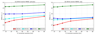
Figure 4 Mean RMSE of vector wind (m s⁻¹) at different model resolutions in (a) January and in (b) July for around 400 radiosonde stations over the globe. Different colours represent different pressure levels (see legend). All the model simulations are based on the standard 1 d forecast configuration shown in Fig. 3. Note that the number of data at the 1000 hPa level might be slightly smaller than at the other pressure levels, as the observations at 1000 hPa are not available when the surface pressure is lower than 1000 hPa.

The RMSE reduction extends throughout the 10 d forecast for the two components of the wind between 1000 and 850 hPa with values around 0.4 m s⁻¹, and it is consistent in both the Northern and Southern Hemisphere and the tropics (not shown). The results are also in agreement with the RMSE with respect to 10 m wind speed from SYNOP observations, with a mean RMSE reduction over the global domain of 0.34 m s⁻¹. The reduction of the mean error is smaller than the RMSE (<0.2 m s⁻¹) throughout the troposphere, which means the largest component of the wind error is random.

3.2 Impact of horizontal resolution on CO₂ diurnal and synoptic variability

The sensitivity of the model skill at hourly and daily timescales to the horizontal resolution of the model is assessed with the error of the CO₂ simulations with respect to hourly mean observations. The change in the RMSE with horizontal resolution based on the surface CO₂ and XCO₂ observations (see Sect. 2.1) is shown in Figs. 5 to 7.

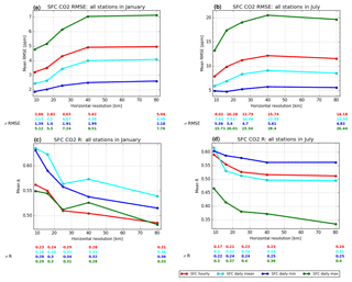
Figure 5 Mean RMSE of near-surface CO₂ (ppm) (a, b) and Pearson's correlation coefficient R (c, d) at different model resolutions in January (a, c) and July (b, d) for all 51 stations (see Table A1). The standard deviation of the plotted variable from each station is shown by the numbers below the horizontal resolution for each temporal resolution (hourly, daily mean, daily min and daily max). All the model simulations are based on the 1 d forecast. Note that different scales are used in each panel.

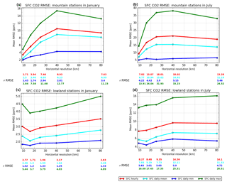
Figure 6 Mean RMSE of near-surface CO₂ (ppm) at different model resolutions in January (a, c) and July (b, d) for (a, b) 37 lowland stations (below 1000 m a.m.s.l.) and (c, d) 12 mountain stations (1000 m a.m.s.l., excluding bao and spo, as listed in Table A1). The standard deviation of the plotted variable from each station is shown by the numbers below the horizontal resolution for each temporal resolution (hourly, daily mean, daily min and daily max). All the model simulations are based on the 1 d forecast. Note that different scales are used in each panel.

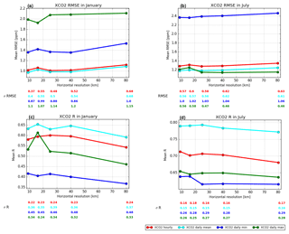
Figure 7 Mean RMSE of XCO₂ (ppm) and Pearson's correlation coefficient R with respect to observations from 18 TCCON stations (see Table A3) at different model resolutions in (a) January and (b) July. The standard deviation of the plotted variable from each station is shown by the numbers below the horizontal resolution for each temporal resolution (hourly, daily mean, daily min and daily max). All the model simulations are based on the 1 d forecast. Note that different scales are used in each panel.

At the surface there is an overall substantial reduction of RMSE between 80 and 9 km (i.e. between 1.8 and 3.5 ppm for hourly data) which is clearly not linear (Fig. 5a and b). The RMSE difference between the 80kmEXP and 40kmEXP simulations or the 40kmEXP and 25kmEXP simulations is not as large as the difference between the higher-resolution simulations (e.g. the 25kmEXP and 16kmEXP or the 16kmEXP and 9kmEXP simulations). This is particularly pronounced for the daily maximum CO₂ occurring usually at night-time, which is generally controlled by local fluxes and small-scale transport of tracers, and therefore it is more sensitive to resolution. The daily maximum values are generally much better captured at 9 km resolution compared to 80 km, with a reduction in the RMSE of around 2.5 ppm in January and 6 ppm in July. Indeed, there are large differences between the RMSE of the daily maximum and minimum CO₂ values. As expected, daily minimum values that emerge during daytime have a smaller RMSE. This is because during daytime the minimum CO₂ values are influenced by the larger-scale fluxes and tracer transport which are less sensitive to high resolution. The reduction in RMSE of the daily minimum CO₂ is therefore smaller than for the daily maximum, but it is still considerable, with an RMSE decrease of around 0.75 ppm from 80 to 9 km resolutions in both January and July. These differences reflect the ability of the model to represent the diurnal cycle. The 9kmEXP simulation clearly shows a general improvement in the CO₂ diurnal cycle near the surface, with smaller differences in the RMSE of the two daily extremes. The largest RMSE reduction comes from mountain sites (over 1000 m a.m.s.l.), ranging between 6 and 10 ppm for hourly CO₂ (Fig. 6a and b), compared to the lowland sites, which can see improvements between 0.5 and 2 ppm for hourly CO₂ RMSE near the surface (Fig. 6c and d).

In general there is also a notable reduction in the spread of the RMSE at the different sites with resolution, as shown by the σ RMSE values below the panels in Figs. 5 and 6. This implies that the spatial gradients between stations are better represented at higher resolutions. The global mean correlation coefficient also increases with resolution from 0.47 to 0.56 in January and 0.51 to 0.59 in July for the hourly CO₂, with consistently higher correlations for the daily mean, minimum and maximum CO₂ at higher resolution.

As expected, the sensitivity to the strategy of sampling the model level at observing stations is generally small over lowlands but large over mountains, particularly at low resolution (Fig. S2). At mountain sites, the model level at the real station height above mean sea level is predominantly in the free troposphere, and therefore it has a small sensitivity to the local fluxes and flow, whereas taking the model level with respect to the model ground generally exhibits larger errors associated with local influences in the boundary layer. The difference between the two sampling strategies in the RMSE and correlation coefficients becomes smaller at high resolution (Fig. S3). This reflects an improvement in the capability of the model to represent the flow and fluxes around complex topography at higher horizontal resolution.

The XCO₂ RMSE at the TCCON sites during daytime also displays a general decrease with resolution (Fig. 7), with differences of the order of 0.1 ppm from 80 to 9 km resolutions and increases in the correlation coefficients (r) of up to 0.05. In boreal summer, the XCO₂ daily minimum has the largest/smallest RMSE/r because it reflects the uncertainty associated with modelled photosynthesis and negative XCO₂ anomalies, whereas in boreal winter, the XCO₂ daily maximum has the largest RMSE because ecosystem respiration associated with positive XCO₂ anomalies is the dominant process at most TCCON sites. It is likely that the larger footprint of XCO₂ (Belikov et al., 2017) at most TCCON stations – associated with its sensitivity to large-scale flux patterns – (Keppel-Aleks et al., 2011, 2012) is causing most TCCON sites to be less sensitive to horizontal resolution. However, there is a large variation in RMSE between sites (see σ RMSE in Figs. 7 and S9), which is reduced at high resolution. In particular, the TCCON site at Pasadena (California, USA), located near the anthropogenic emission hotspot of the megacity of Los Angeles, stands out (Fig. S9). The improvement associated with high resolution at Pasadena is indeed remarkable in January (i.e. approximately 2 ppm RMSE reduction). A more detailed study for Pasadena is provided in Sect. 3.5.

The change of RMSE with resolution is partly associated with the improvement in the transport and also the representation of the local fluxes at higher resolutions. Figure 8 shows that when the fluxes are switched off during the 1 d forecast, there is still an improvement with resolution at most sites, but the magnitude of the error reduction is smaller (see symbols to the right of the dashed line). This is very clear for a large number of mountain sites and TCCON sites affected by anthropogenic emissions such as Pasadena (USA) in January and Saga (Japan) in July. However, there are also some sites and months in which the impact of resolution is better without fluxes than with fluxes (e.g. Pasadena in July). This would indicate that in this case the errors in the fluxes are the main cause of the deterioration in RMSE with resolution.

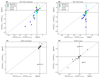
Figure 8 Sensitivity of horizontal resolution impact to surface CO₂ fluxes at (a, b) surface stations and (c, d) TCCON stations in January and July, as shown by the difference in RMSE between different CO₂ tracers, i.e. the standard tracer (RMSE_9 km–RMSE_80 km) and the CO₂ tracer with just transport (RMSE_NFX9km–RMSE_NFX80km) in the y axis and x axis respectively. The symbols that are close to the dashed line correspond to stations that have a small sensitivity to local fluxes, while at the stations associated with symbols that are located above/below the dashed line there is a negative/positive contribution of the local fluxes at high resolution. The further from the dashed line, the larger the contribution of the local fluxes. The stations located along the y axis are mainly impacted by local fluxes. The surface stations in (a, b) are depicted with different symbols depending on whether they are classified as mountain, continental, coastal or remote (see Table A1), while TCCON stations that are strongly influenced by fluxes are labelled with station names. Note that different scales are used in each panel.

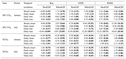
The overall global error statistics of the 9kmEXP and 80kmEXP simulations including the systematic (or bias) error and the standard (or random) error are shown in Table 3. The reduction in RMSE at 9 km is associated with a decrease in the magnitude of the CO₂ biases on average of 1.5 to 2 ppm near the surface and up to 0.2 ppm for XCO₂ and a general reduction in the CO₂ random error of 1 to 1.5 ppm near the surface and 0.1 ppm for XCO₂ (Figs. S4 and S5). The biases depend largely on the bias of the CO₂ initial conditions, as well as the biases of the fluxes and tracer transport. What is important in this sensitivity study is that the standard deviation of the bias at each station – i.e. the inter-station bias – is reduced at 9 km with respect to 80 km, as shown by the shaded area in Figs. S4 and S5. The largest decrease in the inter-station bias between 80kmEXP and 9kmEXP simulations occurs in January, when it is almost halved near the surface. The errors at the individual observing stations are listed in Tables S1, S2, S3 and S4.

Table 3 Surface CO₂ and XCO₂ mean statistics for bias, STDE and RMSE of all stations and the standard deviation of inter-station statistics (in brackets and bold font) from the highest- and lowest-resolution simulations, i.e. 9kmEXP and 80kmEXP respectively. All the SFC CO₂ stations used in January and July are listed in Tables S1 and S2; the TCCON stations used in the XCO₂ statistics are listed in Tables S3 and S4.

3.3 Impact of horizontal resolution on CO₂ forecast error growth

In 10 d the global mean RMSE of CO₂ forecast at the in situ surface stations grows by around 1.4 ppm in January and around 1 ppm in July (Fig. 9). It is worth noting that this error growth is smaller in magnitude than the impact of increasing horizontal resolution from 80 to 9 km. Namely, the 10 d forecast at 9 km is better than the 1 d forecast at 80 km near the surface. At the TCCON sites the XCO₂ RMSE grows on average between 0.2 and 0.5 ppm in 10 d (Fig. 10). The forecast RMSE growth for near-surface CO₂ and XCO₂ does not appear to be linear, with a slow growth until day 4 and a faster increase from day 5 onwards. The CO₂ RMSE growth at 80 km is slightly faster than at 9 km. In summary, the gain in skill from horizontal resolution is maintained throughout the 10 d forecast. Thus, the results suggests that the horizontal resolution has a small but positive impact on the short- and medium-range forecast skill for CO₂ and XCO₂.

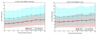
Figure 9 Mean RMSE of near-surface CO₂ (ppm) at different forecast lead times for the 9kmEXP (red) and 80kmEXP (blue) in (a) January and (b) July. The errors are computed with respect to hourly continuous in situ surface measurements from 51 stations (see Table A1). The error standard deviation between the different stations is shown with the shaded area: red for 9kmEXP, blue for 80kmEXP and grey for overlap. Note that different scales are used in each panel.

Figure 10 Same as Fig. 9 but for XCO₂ (ppm). The errors are computed with respect to hourly TCCON observations from 18 TCCON stations (see Table A3).

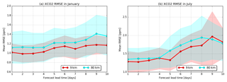
As expected, the RMSE in July is largest because of the high uncertainty associated with the modelled biogenic fluxes at synoptic scales which influence the variability at continental sites (Agustí-Panareda et al., 2014). There is also a larger uncertainty in the meteorology driving the tracer transport during summer compared to winter (Haiden et al., 2017). The fact that the forecast RMSE for day 1 is larger than for day 2 in July is associated with a sporadic overestimation of daily maximum CO₂ peaks at sites influenced by strong local fluxes. There are several potential causes of the overestimation (e.g. biogenic fluxes responding to rapid adjustments in meteorology after analysis re-initialisation at 00:00 UTC or issues with the tracer transport associated with the short spin-up period), but these are beyond the scope of this study.

The near-surface CO₂ RMSE increase during the forecast appears to come mostly from an increase in random error in January and from both mean and random error in July (Fig. S4), whereas for XCO₂, both mean and random errors contribute equally to the forecast RMSE growth in January and July (Fig. S5). This is probably linked to the distribution of the stations, as most in situ stations are located in the Northern Hemisphere, whereas TCCON stations are more equally distributed in both hemispheres, and thus, the mean error at all stations does not show differences between summer and winter conditions.

3.4 Impact of horizontal resolution on CO₂ small-scale variability

The sensitivity of the RMSE to resolution is generally associated with regions that are affected by small-scale variability that cannot be properly represented by typical global tracer transport models (Law et al., 2008; Patra et al., 2008). Figure 11 shows that the mean small-scale variability, given by the standard deviation within 1^∘ × 1^∘ grid box, can be as large as 10 ppm near emission hotspots at the surface during daytime. The representation of the CO₂ small-scale variability at the surface in the 9kmEXP compared to the 80kmEXP is also illustrated in Fig. S6. Larger values than 10 ppm can be found over most land areas at night-time (Fig. 12). These values are likely to be underestimated, since we expect horizontal gradients to become steeper as the resolution increases, the point sources associated with anthropogenic activities become stronger at the grid cell scale and part of the sub-grid-scale flow is resolved.

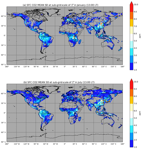
Figure 11 Monthly mean surface CO₂ small-scale variability (σ) within 1^∘ × 1^∘ grid boxes (ppm) at 13:00 local time in (a) January and (b) July. Grey shading denotes σ<1.0.

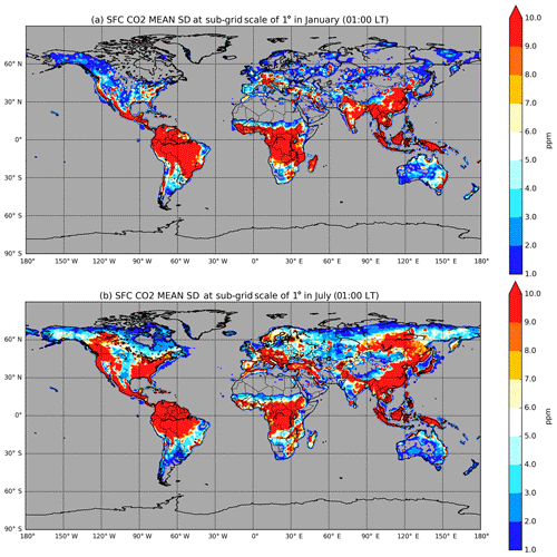
Figure 12 Monthly mean surface CO₂ small-scale variability (σ) within 1^∘ × 1^∘ grid boxes (ppm) at 01:00 local time in (a) January and (b) July. Grey shading denotes σ<1.0.

Coastal sites and mountain sites have a typical sub-grid-scale variability of around 5 ppm during daytime. This variability varies from January to July, depending on meteorological conditions (e.g. stagnant or windy conditions) and the magnitude and sign of fluxes (e.g. biogenic activity shifting northwards in Northern Hemisphere summer). Over land, the patterns of sub-grid-scale variability of surface and total column are consistent (Figs. 11 and 13), as both are subject to surface heterogeneity in terms of topography and fluxes. However, there is a difference in magnitude because the variability of the total column average is much smaller than the variability at the surface.

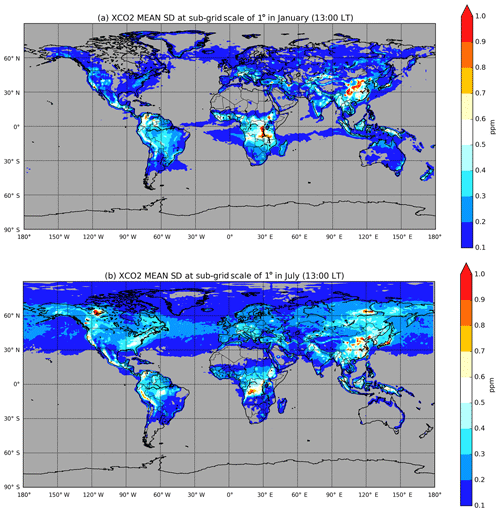
Figure 13 Monthly mean XCO₂ small-scale variability (σ) within 1^∘ × 1^∘ grid boxes (ppm) at 13:00 local time in (a) January and (b) July. Grey shading denotes σ<0.1.

XCO₂ has a maximum standard deviation of 1 ppm near surface flux hotspots and typically less than 0.5 ppm in most regions (Fig. 13), which is consistent with other estimates from regional studies (Corbin et al., 2008; Pillai et al., 2010) (see also Fig. S7 for a visual illustration). The differences in the small-scale XCO₂ variability between day and night appear to be small. Interestingly, the small-scale variability of XCO₂ is much larger in summer than in winter (both in the Northern and Southern Hemisphere). During the growing season, negative CO₂ anomalies associated with plant photosynthesis and positive anomalies associated with ecosystem respiration and anthropogenic emissions combine to create steeper gradients throughout the troposphere – as illustrated in Fig. 1b – that contribute to the enhanced sub-grid-scale variability in summer compared to winter. Over the ocean, the small-scale variability of XCO₂ ranges between 0.1 and 0.3 ppm, with lower values in the winter and higher values in the summer. In the Northern Hemisphere summer, the values over the ocean and over the land are comparable, whereas near the surface, the mean sub-grid-scale variability is an order of magnitude smaller over the ocean than over land. This is because over land the surface fluxes dominate the gradients resulting in the steepest gradients being near the surface, while over the ocean, the transport associated with the weather systems creates steep CO₂ gradients in the free troposphere. Therefore, column-averaged CO₂ is much more likely to be influenced by sub-grid-scale variability associated with weather systems than by surface CO₂ fluxes over the ocean.

3.5 Example of horizontal resolution impact at an urban site

Although the winds, the topography and the spatial heterogeneity of the fluxes are generally better represented at high horizontal resolution, there can still be a deterioration in the RMSE scores at sites where the local influence is strong and the emissions/biogenic fluxes have large errors in the model. In this section we present an example of such a case at the Caltech TCCON site in Pasadena (California, USA; see Table A3) with XCO₂ under clear-sky and daylight conditions. The variability of the simulated XCO₂ exhibits a substantial improvement with high resolution in winter and an equally considerable deterioration in summer (Fig. 15). Thus, it illustrates some of the challenges associated with urban regions.

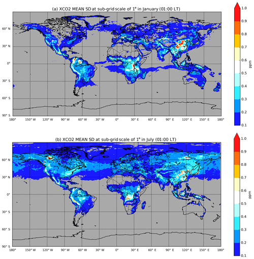
Figure 14 Monthly mean XCO₂ small-scale variability (σ) within 1^∘ × 1^∘ grid boxes (ppm) at 01:00 local time in (a) January and (b) July. Grey shading denotes σ<0.1.

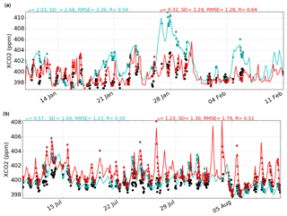
Figure 15 Hourly XCO₂ (ppm) at TCCON site of Pasadena (CA, USA) in (a) January and (b) July from 80kmEXP (blue) and 9kmEXP (red) simulations. Hourly observations are shown by black circles. Triangles represent the model XCO2 after smoothing with TCCON averaging kernel and prior. The bias (μ), standard error (STDE) and Pearson's correlation coefficient (R) from 80kmEXP (blue) and 9kmEXP (red) are shown at the top of each panel.

Pasadena is located 14 km north-east of the megacity of Los Angeles (LA) with a large local anthropogenic emission influence (Wunch et al., 2009; Newman et al., 2016). The XCO₂ variability in the model is also mainly explained by the local anthropogenic emissions (Figs. S10 and S11) producing very large CO₂ enhancements in the planetary boundary layer (PBL) (Fig. S12) and therefore in XCO₂. The CO₂ budget of the anthropogenic emissions used at 9 and 80 km is the same. However, the instantaneous values of the emissions per square metre are much higher at 9 than at 80 km, representing some of the steep gradients and heterogeneous distribution of fossil fuel emissions within the LA basin, with higher emissions in downtown LA and lower emissions in Pasadena (e.g. Feng et al., 2016). At 80 km, Pasadena and downtown LA are in the same model grid box, which means this gradient cannot be represented. In addition to the influence of anthropogenic emissions, the seasonal variation of the winds is very pronounced in Pasadena, with a large contrast in the origin or air masses between winter and summer (Verhulst et al., 2017).

In winter, air masses originate from various directions: from the prevailing westerly and southerly winds, bringing and accumulating polluted air from the LA megacity, to northerly and easterly flow, characterised by cleaner air with lower CO₂ values from the surrounding desert and mountains (Newman et al., 2016). Persistent low wind conditions lead to a large accumulation of CO₂ in the LA basin as it remains trapped by the mountains. These episodes result in large enhancements in XCO₂ (Hedelius et al., 2017) and high CO₂ anomalies over periods of a few days (e.g. 26 to 30 January in Fig. 15a). In those stagnant conditions, the 9kmEXP simulation is in much closer agreement with the observed XCO₂ peaks than the 80kmEXP simulation, which overestimates the XCO₂ anomalies. This is because at 80 km resolution there is an effectively uniform emission for the whole LA basin. Note that the CO₂ and XCO₂ small-scale variability around LA appears to be larger in winter than in summer (Figs. 11 and 14). Without preserving the sharp gradient in emissions between Pasadena and downtown LA, the CO₂ accumulation is overestimated in Pasadena.

The atmospheric circulation in summer is mainly controlled by the sea–mountain breeze (Lu and Turco, 1994). Daytime advection of anthropogenic CO₂-rich air from the city of LA results in XCO₂ peaking in the afternoon before it is vented over the mountains (Newman et al., 2013, 2016). The overestimation in the summer XCO₂ peaks at 9 km likely reflects an overestimation of the emissions in downtown LA. The enhancement of CO₂ from anthropogenic emissions is larger at 9 than at 80 km (Fig. S11). This suggests an overestimation of the hotspot emissions over the LA basin in the temporally extrapolated EDGAR inventory, which is smoothed and less noticeable at lower resolution. There are many reasons why the anthropogenic emissions used in the model can be overestimated, including the temporal extrapolation based on country-scale scaling factors and the use of annual constant emissions in EDGAR v4.2 FT2010 instead of seasonally varying emissions (Corbin et al., 2010).

Differences in the sampling location (centre of grid is 3 and 34 km from station location at 9 and 80 km respectively) and orography (15 m below and 46 m below the station height at 9 and 80 km respectively), as well as differences in flow and local biogenic fluxes can also play a role in explaining the differences between the simulations at 80 and 9 km resolutions. The results are consistent with previous studies by Feng et al. (2016) and Hedelius et al. (2018). They found that uncertainties in the fluxes and their high-resolution representation in the LA basin are as important as the atmospheric tracer transport in the representation of the CO₂ enhancement and its variability in Pasadena.

This example at Pasadena highlights the importance of horizontal resolution in representing local gradients of CO₂ fluxes in order to reduce the atmospheric CO₂ representativeness error. It emphasises that the impact of increasing horizontal resolution is not only to reduce the error of atmospheric CO₂ simulations but to enhance the sensitivity of the modelled atmospheric CO₂ variability to the CO₂ fluxes in urban regions characterised by emission hotspots. Therefore horizontal resolution is crucial for atmospheric inversion systems that aim to estimate anthropogenic emissions.

4 Discussion and conclusions

This paper addresses the importance of horizontal resolution in the representation of CO₂ variability at diurnal and synoptic scales, referred to here as CO₂ weather. The CO₂ simulations performed with the ECMWF IFS model allow the combined impact of horizontal resolution associated with (i) the online modelling of the winds, (ii) the numerical tracer transport model and (iii) the spatial–temporal distribution of CO₂ fluxes over land to be quantified. The assessment is done by comparing the model errors at various horizontal resolutions with respect to a wide range of observations with hourly resolution and distributed around the globe. The horizontal resolution of the model ranges from 9 km – as in current operational high-resolution weather and CO₂ forecasts at ECMWF – to 80 km, which corresponds to the ERA-Interim Reanalysis resolution, widely used by many offline tracer transport models. The conclusions to the three main questions addressed in the paper are summarised below.

1. What is the sensitivity of the modelled atmospheric CO₂ variability at diurnal and synoptic timescales to horizonal resolution?

   The high horizontal resolution of 9 km leads to a general improvement in the simulated variability of hourly near-surface and column-averaged atmospheric CO₂ compared to the resolution of 80 km. This is shown by a reduction in the mean RMSE of around 1.8 ppm in winter and 3.5 ppm in summer (equivalent to 33 % error reduction) and 0.1 ppm (i.e. around 10 % error reduction) at in situ and TCCON sites respectively, which is associated with a reduction of both the mean and random errors in the model. The inter-station variability is also generally improved in the 9kmEXP simulation for near-surface and column-averaged CO₂ in January and July, with the standard deviation of station biases reduced up to 50 % compared to the 80kmEXP simulation in January for near-surface CO₂.

   Column-averaged CO₂ is not as sensitive to horizontal resolution as near-surface CO₂ because it has a larger footprint or area of flux influence, except for sites like Pasadena which are close to CO₂ emission hotspots. Similarly, minimum daily values of atmospheric CO₂ are less sensitive to the horizontal resolution than maximum daily values because their footprint tends to be larger in size.

   This study also shows that the RMSE reduction with horizontal resolution is not linear. This implies that results from sensitivity studies exploring the impact of resolution based on coarse simulations which show small sensitivity to horizontal resolution cannot be extrapolated to higher horizontal resolutions. These results are consistent with the findings of the Lin et al. (2017) study based on a wider range of model resolutions from ∼100 down to 1 km and observations at three mountain sites. The reduction in model error associated with the increase of horizontal resolution to 9 km emanates from four different well-known and connected aspects, as listed below.

   • a.

     Better accuracy of the horizontal winds is integral to the reduction of error. The strength of the winds determines the observed CO₂ variability – i.e. the detected CO₂ enhancement – close to emission hotspots like in urban regions (Newman et al., 2013; Xueref-Remy et al., 2018). Therefore, the error in the wind will affect the value of the enhanced CO₂ as much as the error in the fluxes. In this context, for example, a wind speed error reduction of 0.5 m s⁻¹ – as shown in Sect. 3.1 – across a gradient of 10 ppm per degree – typical of urban areas as shown in Sect. 3.4 – throughout a 6 h period can result in a CO₂ error reduction of around 1 ppm. Uncertainty in the winds has been shown to be one of the largest contributors to the uncertainty in the estimated fluxes over urban areas (e.g. Hedelius et al., 2018).

   • b

     An overall reduction of the numerical error associated with lower spatial and temporal truncation errors leads to a reduction in tracer advection errors (Prather et al., 2008).

   • c.

     There is a general improvement in the horizontal and vertical sampling at the station locations in the model associated with a more realistic representation of orography and coastal boundaries.

   • d.

     A more realistic representation of CO₂ flux distribution at the surface is key. High resolution gives an increased capability to represent small-scale sharp gradients associated with complex topographical boundaries at coastal and mountainous terrain sites, as well as the presence of strong local surface fluxes of CO₂ such as anthropogenic emission hotspots.

2. How is the horizontal resolution affecting the forecast error growth of atmospheric CO₂?

   The horizontal resolution has a consistent positive impact on the error reduction at all forecast lead times, from day 1 to day 10, implying a long-lived improvement in the prediction skill. The RMSE growth is small from days 1 to 4, namely less than 0.5 ppm near the surface CO₂ and less than 0.05 ppm for XCO₂. Over the 10 d there is an increase in RMSE of 1 to 1.5 ppm at the surface and 0.1 to 0.5 ppm for the total column. This error growth is not linear. For example, in July the error of the 1 d forecast is worse than the 2 d forecast, with a slower error increase during the 2 to 4 d forecast and a generally faster error increase from day 5 to day 10 in the forecast. This incoherent change in the error evolution at the beginning of the forecast is likely linked to the strong influence of the biogenic surface fluxes, which respond very fast to changes in temperature, moisture and radiation forcing in the model. Inconsistencies between the initial conditions from the analysis and the model forecast can cause spin-up adjustments which may lead to a degradation of the 1 d forecast.

   Generally, the improvement of forecast skill with increased horizontal resolution is most pronounced in January, when at 9 km resolution the skill of the 10 d forecast is better or equal to the accuracy of the 1 d forecast at 80 km both near the surface and for the column average CO₂. It is likely that the skill of the 10 d forecast to represent variability of CO₂ during summer conditions is hampered by the growing errors in the surface biogenic fluxes during the forecast, as they can be an important contributor to synoptic variability in the summer (Agustí-Panareda et al., 2014).

3. Where and when are the typical representativeness errors associated with unresolved small-scale variability largest?

   During daytime, the CO₂ small-scale variability of the 9 km resolution forecast ranges from 1 to 10 ppm at the surface and is an order of magnitude smaller (0.1 to 1 ppm) for the total column average. It points to the areas associated with small-scale gradients where horizontal resolution matters: coastal boundaries and mountain regions have typical values of 5 ppm per degree, and CO₂ flux hotspots have the highest variability of up to 10 ppm per degree. During night-time, the small-scale variability tends to be larger than 10 ppm over most areas near the surface, whereas that of column-averaged CO₂ shows small differences between day and night.

   The high horizontal resolution gives us an insight into the areas with high sensitivity to uncertainty associated with both local tracer transport and fluxes. It is in these areas where improvements in the tracer transport and increased understanding of the heterogeneity and complexity of the surface will be crucial in future model developments. Since these areas are close to emission hotspots, it is clear that in order to monitor CO₂ emissions, particularly from cities and power stations such as in the new Carbon Human Emission project (http://www.che-project.eu, last access: 30 May 2019), it is paramount to invest in high horizontal resolution models.

   Interesting differences are found between surface and column-averaged variability. Near the surface the variability is most pronounced close to emission hotspots and complex terrain. For column-averaged CO₂ the sub-grid-scale variability is also substantial over the ocean downstream from emissions. This emphasises the importance of the transport influence on XCO₂ variability. Small-scale variability is also found to be more pronounced in summer than in winter, as biogenic CO₂ fluxes of opposite sign in summer enhance the CO₂ gradients in the atmosphere.

In summary, this paper has shown that model simulations using the CAMS CO₂ forecasting system at 9 km resolution can provide a more accurate representation of tracer transport and the local influences of surface fluxes than at lower resolutions ranging from 80 to 16 km, resulting in an overall better representation of the atmospheric CO₂ variability at diurnal and synoptic timescales. However, at higher horizontal resolution there is also higher sensitivity of atmospheric CO₂ to CO₂ flux errors, as emissions and biogenic flux hotspots are not diffused over large areas like in lower-resolution models. Thus, higher-resolution models also risk deterioration in the forecast RMSE, e.g. near emission hotspots associated with larger errors. With the enhancement of the model uncertainty at high resolution, the prospect of further increasing the horizontal resolution needs to be carefully balanced with improvements in the most uncertain model processes.

The impact of horizontal resolution on the accuracy of the winds highlights that errors in the wind need to be considered as an important source of uncertainty both in the atmospheric CO₂ analysis and forecast and in the inversion systems (Polavarapu et al., 2016). The findings in this study also suggest that increasing horizontal resolution up to kilometric scales in atmospheric data assimilation and inversion systems would allow the use of more in situ and high-resolution satellite observations close to strong sources and sinks and over complex terrain. Lin et al. (2017) found that a minimum horizontal resolution of 4 km is required to simulate a realistic diurnal cycle of CO₂ at mountain sites.

Currently, the precision of XCO₂ from satellite observations is around 1.0 to 1.5 ppm for ACOS-GOSAT data (O'Dell et al., 2012) and OCO-2 data (Wunch et al., 2017). However, if tracer transport models cannot represent their variability accurately in space and time, all the efforts to reduce the errors from the satellite retrievals of CO₂ will not be fruitful in their attempt to reduce the uncertainty in the estimation of surface fluxes. This is because relatively small differences in atmospheric mixing ratios are associated with significant differences in surface fluxes (Houweling et al., 2010; Ott et al., 2015). The benefits of high resolution in inversion systems will also need to be balanced with the costs of running a model at such high resolution.

Finally, the CAMS high-resolution forecast running currently at 9 km resolution can provide benchmarks for other simulations using coarser grids or offline meteorology (Yu et al., 2018). Both CAMS analysis and high-resolution forecasts are freely available to users (https://atmosphere.copernicus.eu, last access: 30 May 2019). Potential applications include the estimation of representativeness errors and data selection screening of observations from satellites and in situ stations in data assimilation systems, spatial collocation of XCO₂ from satellite and TCCON data for validation purposes (e.g. Guerlet et al., 2013) or as boundary conditions for high-resolution simulations and/or inversions at regional scales.

Appendix A

Worthy et al. (2003)Peterson et al. (1986)Worthy et al. (2003)Hatakka et al. (2003)Worthy et al. (2003)Worthy et al. (2003)Worthy et al. (2003)Ramonet et al. (2010)Wilson (2013)Vermeulen et al. (2011)Worthy et al. (2003)Worthy et al. (2003)Worthy et al. (2003)Worthy et al. (2003)Necki et al. (2003)Rozanski et al. (2014)Schmidt et al. (2003)Haszpra et al. (2001)Schibig et al. (2015)Andrews et al. (2014)Lopez et al. (2015)Andrews et al. (2014)Worthy et al. (2003)Worthy et al. (2003)Morguí et al. (2013)Worthy et al. (2003)Morguí et al. (2013)Stephens et al. (2011)Stephens et al. (2011)Morguí et al. (2013)Stephens et al. (2011)Andrews et al. (2014)Tsutsumi et al. (2005)Andrews et al. (2014)Andrews et al. (2014)Morguí et al. (2013)Andrews et al. (2014)Andrews et al. (2014)Gomez-Pelaez and Ramos (2011)Tsutsumi et al. (2005)Tsutsumi et al. (2005)Thoning et al. (1989)Halter et al. (1988)Brunke et al. (2004)Gaudry et al. (1991)Francey et al. (2003)Stavert et al. (2018)Loh et al. (2017)Conway and Thoning (1990)

Table A1 Continuous in situ stations (surface and tower) used to evaluate synoptic variability. NA denotes references that are not available. The full names for the abbreviations of the network organisations are provided in Table A2.

Table A2 Organisations associated with observing stations.

Deutscher et al. (2014)Notholt et al. (2014a)Hase et al. (2014)Warneke et al. (2014)Sussmann and Rettinger (2014)Wennberg et al. (2014a)Morino et al. (2017a)Wennberg et al. (2016)Morino et al. (2014b)Iraci et al. (2016)Wennberg et al. (2014b)Shiomi et al. (2014)Blumenstock et al. (2014)Feist et al. (2014)Griffith et al. (2014a)De Mazière et al. (2014)Griffith et al. (2014b)Sherlock et al. (2014)

Table A3 TCCON stations