the Creative Commons Attribution 4.0 License.
the Creative Commons Attribution 4.0 License.
 | 24 May 2019
Simulation of the radiative effect of haze on the urban hydrological cycle using reanalysis data in Beijing
Sue Grimmond
Sonja Murto
Huizhi Liu
Anu-Maija Sundström
Leena Järvi
Although increased aerosol concentration modifies local air temperatures and boundary layer structure in urban areas, little is known about its effects on the urban hydrological cycle. Changes in the hydrological cycle modify surface runoff and flooding. Furthermore, as runoff commonly transports pollutants to soil and water, any changes impact urban soil and aquatic environments. To explore the radiative effect of haze on changes in the urban surface water balance in Beijing, different haze levels are modelled using the Surface Urban Energy and Water Balance Scheme (SUEWS), forced by reanalysis data. The pollution levels are classified using aerosol optical depth observations. The secondary aims are to examine the usability of a global reanalysis dataset in a highly polluted environment and the SUEWS model performance.
We show that the reanalysis data do not include the attenuating effect of haze on incoming solar radiation and develop a correction method. Using these corrected data, SUEWS simulates measured eddy covariance heat fluxes well. Both surface runoff and drainage increase with severe haze levels, particularly with low precipitation rates: runoff from 0.06 to 0.18 mm d−1 and drainage from 0.43 to 0.62 mm d−1 during fairly clean to extremely polluted conditions, respectively. Considering all precipitation events, runoff rates are higher during extremely polluted conditions than cleaner conditions, but as the cleanest conditions have high precipitation rates, they induce the largest runoff. Thus, the haze radiative effect is unlikely to modify flash flooding likelihood. However, flushing pollutants from surfaces may increase pollutant loads in urban water bodies.
- Article
(5000 KB) - Full-text XML
- BibTeX
- EndNote


In recent decades rapid economic development and the acceleration of urbanization and industrialization have led to many environmental problems in China, such as increased atmospheric aerosol concentrations, water pollution, and soil contamination (e.g. Kulmala, 2015; Liao et al., 2015; Shao et al., 2006; Sun et al., 2014; Xia et al., 2011). As a consequence of urbanization and industrialization, north-east China is one of the most populated and polluted areas in the world (HEI International Scientific Oversight Committee, 2010). With continuing urbanization, serious water shortages and deterioration of aquatic environment are becoming major concerns for municipal hydrological authorities (Li et al., 2015; Sun et al., 2014). As urbanization increases the extent of impervious surfaces, enhancing the likelihood of surface floods from surface runoff (e.g. Rodriguez et al., 2003), understanding the local urban hydrological cycle, potential increase in surface flooding, and pollutant loads to urban water bodies is important.
Increased aerosol concentration modifies local urban climate by decreasing solar radiation received at the surface and thus decreasing near-surface air temperatures (Ding et al., 2013; Wang et al., 2014), turbulent heat fluxes, and boundary layer heights but increasing incoming longwave radiation emissions from the polluted atmosphere (Miao et al., 2009; Petäjä et al., 2016; Tang et al., 2016). Increased absorption of radiation by the polluted atmosphere changes the vertical temperature profile, leading to more stable conditions (Petäjä et al., 2016). With reduced turbulence and mixing, the boundary layer height is lower (Petäjä et al., 2016), which increases the near-surface pollutant concentrations. With less energy available at the surface, because of the attenuated incoming solar radiation, evaporation may be reduced, modifying other water balance terms. In addition, haze can increase the condensation nuclei and therefore precipitation. The higher surface runoff rates due to the modified water balance may increase pollutant loads in urban water bodies, by flushing pollutants from contaminated surfaces. However, the linkage between increased aerosol concentrations and the urban hydrological cycle has not yet been studied at the local scale, despite its potential contribution to deterioration of the urban aquatic environment. This may be because of a lack of high-resolution meteorological and/or hydrological observations for detailed analyses and modelling from regions with heavy air pollution episodes. Global reanalysis products could provide the essential variables to enable modelling where necessary observations are unavailable or have too coarse a temporal resolution (Kokkonen et al., 2018b). A number of reanalysis products are available, but to the best of our knowledge none have been properly evaluated in highly polluted urban environments. Poor air quality is the result of several factors, including pollutant emissions, atmospheric transport, atmospheric chemistry, and meteorological conditions. Therefore the accuracy of meteorological variables in reanalysis products is essential to be able to study the effects of pollutants on the local hydrological cycle correctly.
The aims of this study are (1) to evaluate the 2006 to 2009 WATCH Forcing Data ERA-Interim (WFDEI; Weedon et al., 2014) reanalysis data using observations in the highly polluted city of Beijing, China (Sect. 3.1), (2) to evaluate the urban land surface model Surface Urban Energy and Water Balance Scheme (SUEWS; Järvi et al., 2011; Ward et al., 2017) using eddy covariance flux measurements of latent and sensible heat for 2006–2009 (Sect. 3.2), and (3) to simulate how increased aerosol concentrations modify the local urban hydrological cycle for the period 2001–2013 using SUEWS (Sect. 3.3). Aerosol optical depth observations are used to classify the pollution levels for the assessment of the impact of the radiative effect of haze on the local urban water balance in Beijing for 2001–2013. The broader impacts of changes in water balance on local aquatic environment are discussed in Sect. 4.
In this study the changes in the hydrological cycle are assumed to be caused mainly by the changes in the surface energy balance due to the attenuated incoming solar radiation and the changes in the precipitation rates provided by the reanalysis data, which further modifies the water balance. The effects of, for example, a vapour pressure deficit and changes in soil water storage (i.e. availability of water) are not discussed.
The hydrological modelling is conducted using the Surface Urban Energy and Water Balance Scheme (SUEWS; Järvi et al., 2011) version V2017b (Ward et al., 2017, 2018). SUEWS is an urban land surface model that simulates the surface energy and water balances at the local (neighbourhood) scale. In SUEWS, the urban surface is separated into seven hydrologically connected surface types (buildings, paved surfaces, grass, evergreen trees/shrub, deciduous trees/shrubs, and water), with a single soil layer below (excluding the water surface). For each surface type, evaporation is calculated using the Penman–Monteith equation (Monteith, 1965; Penman, 1948) modified for urban environments (Grimmond and Oke, 1991) and runoff from a running water balance (Grimmond and Oke, 1991; Järvi et al., 2011). SUEWS has been optimized to run with a minimum amount of model forcing data and includes sub-models for net all-wave radiation, irrigation, and anthropogenic heat flux. The meteorological input variables needed are wind speed, relative humidity, air temperature, pressure, precipitation, and incoming solar radiation. The overall parameters used in the model runs are given in Table 1. The performance of SUEWS and the sensitivity to input variables and parameterization have been extensively evaluated in past studies in different climates and for multiple variables (e.g. Alexander et al., 2015; Ao et al., 2016, 2018; Demuzere et al., 2017; Järvi et al., 2011, 2014, 2017; Karsisto et al., 2016; Kokkonen et al., 2018a, b; Ward et al., 2016, 2018).
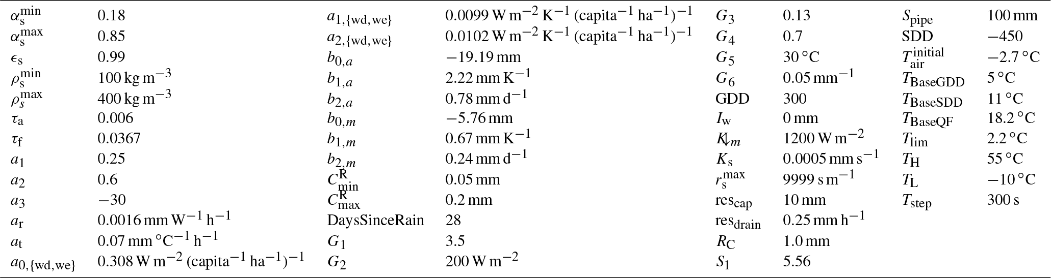
Table 1Overall model parameter values used in model runs in Beijing. See Table A1 in the Appendix for notation and Järvi et al. (2011, 2014) and Ward et al. (2016) for data sources.
The study area is a 1 km radius circle around the 325 m high Institute of Atmospheric Physics (IAP) meteorological measurement tower (39.97∘ N, 116.37∘ E) located in the north-western part of Beijing, China, in Haidian District (Liu et al., 2012). This circle approximates the source area of the eddy covariance (EC) measurements at height 47 m (Liu et al., 2012) used to evaluate SUEWS model performance. This area is a densely built (70 % impervious surfaces) urban area (Local Climate Zone (LCZ) 1; Stewart and Oke, 2012), with only 29 % vegetated surfaces and 1 % open water. The surface cover fractions for the study area are calculated from aerial photographs using GIS software (ArcGIS 10.1) and digitalized using two freely available base maps: OpenStreetMap (OpenStreetMap contributors, 2015) and World Imagery, with 1 m spatial resolution (Esri, 2009), following the methods in Murto (2017). The OpenStreetMap has substantial gaps, especially in the southern part of the study area. Therefore two sources of spatial data are used, which enables evaluation of the existing data in the areas where the two sources could be compared. With the available imagery, separation of evergreen and deciduous trees and shrubs needed by the model is not possible using GIS methods. Therefore these fractions (15 % and 85 % of fraction of vegetation, respectively) together with mean tree height (8 m) are estimated based on common tree species found in Haidian District (Ma and Liu, 2003). The mean building height is 19.1 m (Miao et al., 2012).
The population density is estimated from a 1 km gridded population dataset for 2010 (Fu et al., 2014). The grid population densities are weighted by their areal fractions within the study area. There has been no further urbanization at the study site (Cheng et al., 2018), and therefore population density and surface characteristics are assumed to stay constant throughout the study period.
The WFDEI (Weedon et al., 2014) meteorological forcing data are derived for hydrological modelling purposes from the ERA-Interim (Dee et al., 2011) reanalysis product via sequential interpolation to half-degree resolution with 3 h temporal resolution. Bias correction with quantile mapping (BCQM) is applied to downscale the daily precipitation totals (Kokkonen et al., 2018b). The 5 min time-step calculations are disaggregated in a non-linear manner to provide realistic precipitation patterns from coarse input data (Ward et al., 2018) (Table A3). The air temperature (Tair) and pressure are adjusted to simulation height using the environmental lapse rate ( K km−1) and the hypsometric equation (Kokkonen et al., 2018b; Weedon et al., 2010). The WFDEI data are downscaled from 3 h to 5 min temporal resolution of the model time step within the model (Ward et al., 2017).
The WFDEI reanalysis data in Beijing are evaluated for 2006–2009 using observed meteorological variables, including hourly Tair, relative humidity (RH), and incoming solar radiation (K↓) measured on the IAP tower at the 47 m level (Liu et al., 2012) (Table 2) and daily precipitation (P) 10 km south-west of the tower (Menne et al., 2012a, b). The same years are used to evaluate SUEWS against the IAP EC measurements from the same 47 m level. The 47 m level of the IAP tower is in the roughness sublayer for wind directions mainly from the south-west and north-west (Miao et al., 2012). Therefore the wind directions with buildings over 50 m high (314–3, 40–45, 112–128, 160–243∘) are filtered out from the EC observations (34 % of the data).
Table 2Instruments used on the 325 m IAP tower (47 m level; Liu et al., 2012).

SUEWS is run for 2000 to 2013, with the first year as a spin-up period, leaving years 2001–2013 for the analysis. The hydrological cycle is analysed during the thermal summer (April–September) as the wintertime in Beijing is extremely dry. For example in 2013 the precipitation that occurred between October and March only covers 6 % (33.7 mm) of the annual precipitation (Beijing Municipal Bureau of Statistics, 2016). Due to a difference in behaviour in summer and winter months, the two periods should be analysed separately, and this would leave an insufficient amount of data for statistical analysis in winter months. The polluted and non-polluted days in the studied years are separated based on aerosol optical depth (AOD; 440 nm) obtained from the AERONET station (Che et al., 2009; Holben et al., 1998) located at the study site.
Statistical methods
The pollution levels are obtained by dividing the AOD observations from the whole study period (2001–2013) into four quantiles (i.e. roughly equal amount of data in all of the air quality classes), i.e. extremely polluted air (AOD>1), polluted air (0.438–1), slightly polluted (0.203–0.438), and fairly clean air (<0.203).
The hydrological analysis is done by stratifying the results by the different pollution levels described above and different percentiles of daily precipitation from the study period (2001–2013). The hydrological components are divided into four ranges of daily precipitation percentiles (0–25, 0–50, 0–75, 0–100) including dry days. Statistical analysis of the results of P (stratified already by different percentiles) includes wet days only, but the other variables analysed also include the dry days.
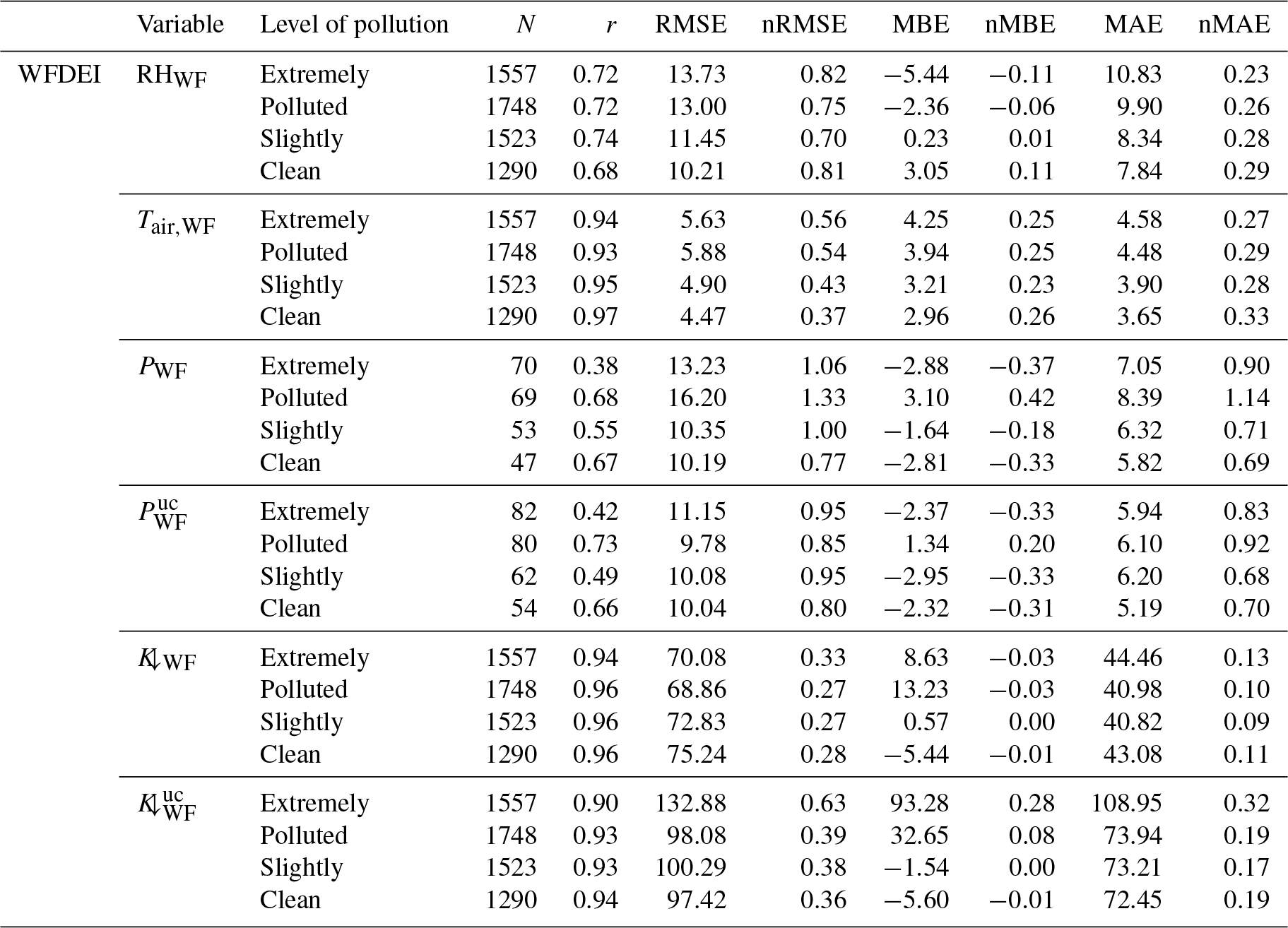
Table 3Comparison for 2006–2009 of WFDEI meteorological variables with observations, stratified by pollution level (extremely polluted air (AOD>1), polluted air (0.438–1), slightly polluted air (0.203–0.438), and fairly clean air (<0.203); see “Statistical methods” for details). Data are hourly – relative humidity (RH, %), air temperature (Tair, ∘C), and incoming solar radiation (K↓, W m−2) – and daily – precipitation (P, mm d−1). The superscript “uc” indicates uncorrected variables. For explanation see “Statistical methods”.
Box plots (Figs. 4, 7, and A2 in the Appendix) give the median and the interquartile range (IQR) with whiskers of 1.5 IQR. The box plots have notches which indicate the 95 % confidence levels.
The linear correlations among different variables in Tables 3 and 5 are analysed using common statistical tools, including the root mean square error (RMSE), RMSE normalized with standard deviation of observations (nRMSE), mean bias error (MBE), MBE normalized with mean of observations (nMBE), mean absolute error (MAE), MAE normalized with mean of observations (nMAE), and Pearson's correlation coefficient (r). The regression lines have been calculated for scatter plots (Figs. 1 and A1) after applying LOWESS smoothing (Cleveland, 1979, 1981). The performance of model runs and WFDEI variables is evaluated using a Taylor (2001) diagram (Fig. 5).
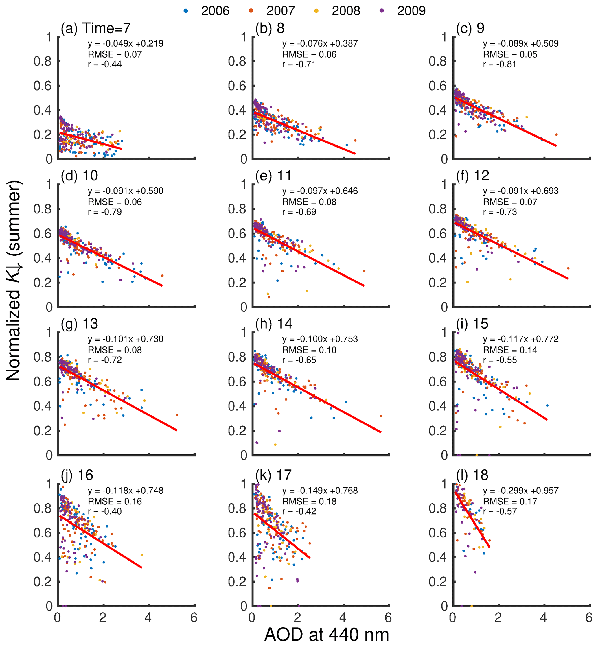
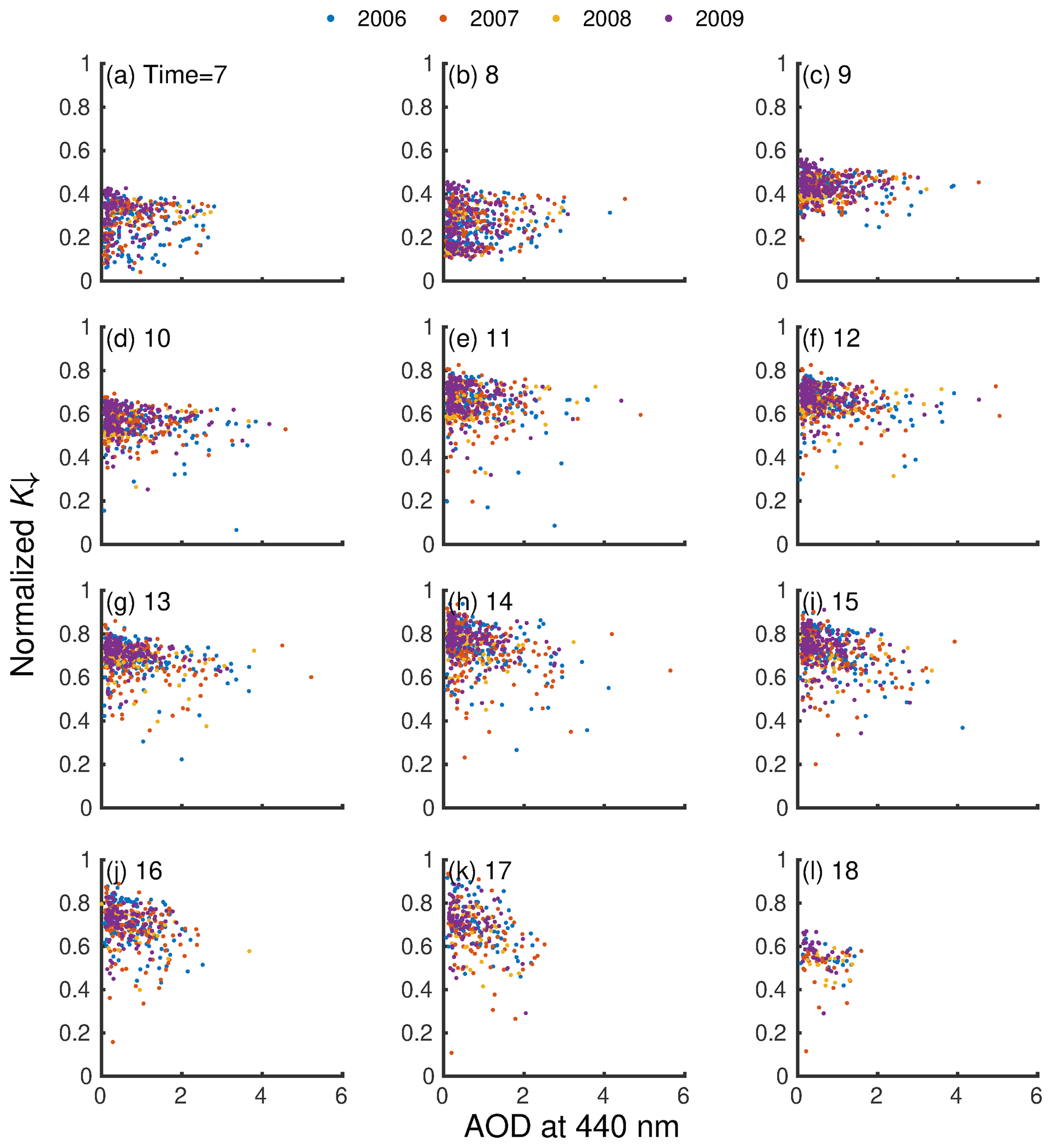
Figure 1Observed hourly incoming solar radiation (K↓) normalized with clear-sky radiation (ISC×cos θz) against aerosol optical depth (AOD) observations (Holben et al., 1998) for different hours of the day (a–l) for thermal summer months (April–September) at the 325 m IAP meteorological tower (47 m level; Liu et al., 2012). Winter months in Fig. A1. Linear regression (red line) is fit after LOWESS smoothing is applied for the scatter. See “Statistical methods” for more details.
3.1 Evaluation of WFDEI data in polluted urban environment
Although extensive evaluation of WFDEI data has been undertaken (e.g. Weedon et al., 2014), polluted urban areas have been neglected so far. Here WFDEI P, K↓, RH, and Tair (hereafter the subscript “WF” indicates WFDEI variables), the most important input variables for hydrological modelling with SUEWS (Alexander et al., 2015; Kokkonen et al., 2018b; Ward and Grimmond, 2017), are evaluated.
Haze is known to attenuate K↓ in highly polluted environments, but this attenuation is not properly accounted for in the WFDEI data (Figs. 1 and 2, Table 3) because sometimes haze may be from local emissions and because of secondary nucleation. Overestimation of hourly K↓WF against the observed values increases with the level of pollution (nMBE: −0.01, 0.00, 0.08, 0.28; fairly clean, slightly polluted, polluted, and extremely polluted air, respectively; see “Statistical methods” for details). Thus hourly K↓WF is corrected using observations between 2006 and 2009 from the 325 m IAP measurement tower separately for thermal summer (April–September) and winter (October–March) due to slightly different behaviour (Figs. 1 and A1). First LOWESS smoothing is applied to observed K↓ normalized with the clear-sky radiation (determined from ISC×cos θz, where ISC is the solar constant (1367 W m−2) and θz is the solar zenith angle) as a function of AOD. Second, regression coefficients for different times of the day are determined (Fig. 1). Before corrections are applied to WFDEI data, the K↓WF is downscaled from 3 to 1 h temporal resolution (Kokkonen et al., 2018b). The corrections are made by fitting the hourly K↓WF data for the whole study period (2001–2013) using regression coefficients when AOD observations are available (N=20 462). The developed correction increases the K↓WF accuracy substantially during haze events, bringing the more polluted levels closer to the cleaner levels (nMBE: −0.01, 0.00, −0.03, and −0.03 from clean to extremely polluted conditions; before correction nMBE: −0.01, 0.00, 0.08, and 0.28).
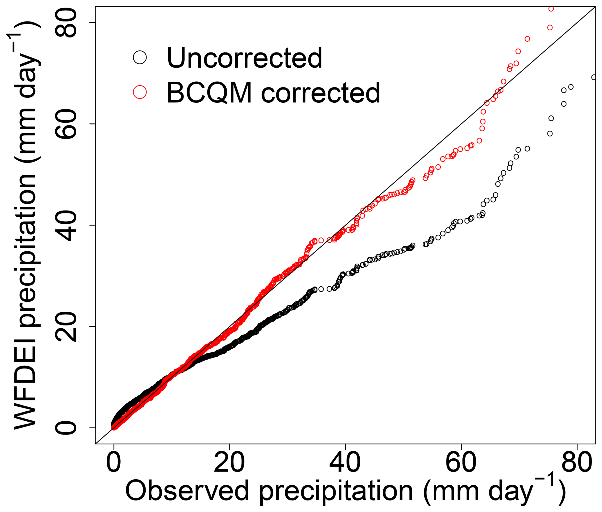
Figure 3Quantile–quantile plot of uncorrected WFDEI precipitation and WFDEI precipitation bias corrected using quantile mapping (BCQM; Kokkonen et al., 2018b) versus observed precipitation (1980–2012).
The height-corrected Tair,WF (Kokkonen et al., 2018b) correlates with observations well (r>0.93), and the nMBE is low (up to 0.26; Table 3). The nMBE of RHWF is also low (from −0.11 to 0.11) and the correlation coefficient reasonably good (>0.68). Thus, these reanalysis variables are assumed to already include the effect of haze.
The WFDEI precipitation is higher than observed for days with <11 mm d−1 of precipitation but too low for higher (>11 mm d−1) daily rainfall rates (Fig. 3). After the BCQM correction (Kokkonen et al., 2018b) the correspondence with observations is generally improved (Fig. 3), as found previously in Vancouver and London (Kokkonen et al., 2018b). However, PWF statistics (Table 3) during extremely polluted and polluted levels become slightly poorer (r: from 0.42 to 0.38 and 0.73 to 0.68; nRMSE: from 0.95 to 1.06 and 0.85 to 1.33, respectively), whereas they mainly improve with slightly polluted and fairly clean pollution levels (r: from 0.49 to 0.55 and 0.66 to 0.67; nRMSE: from 0.95 to 1.00 and 0.80 to 0.77, respectively). It is expected that the correction affects mostly cleaner conditions since most of the larger daily totals of precipitation occur during periods of slightly polluted and fairly clean air (Fig. 4).
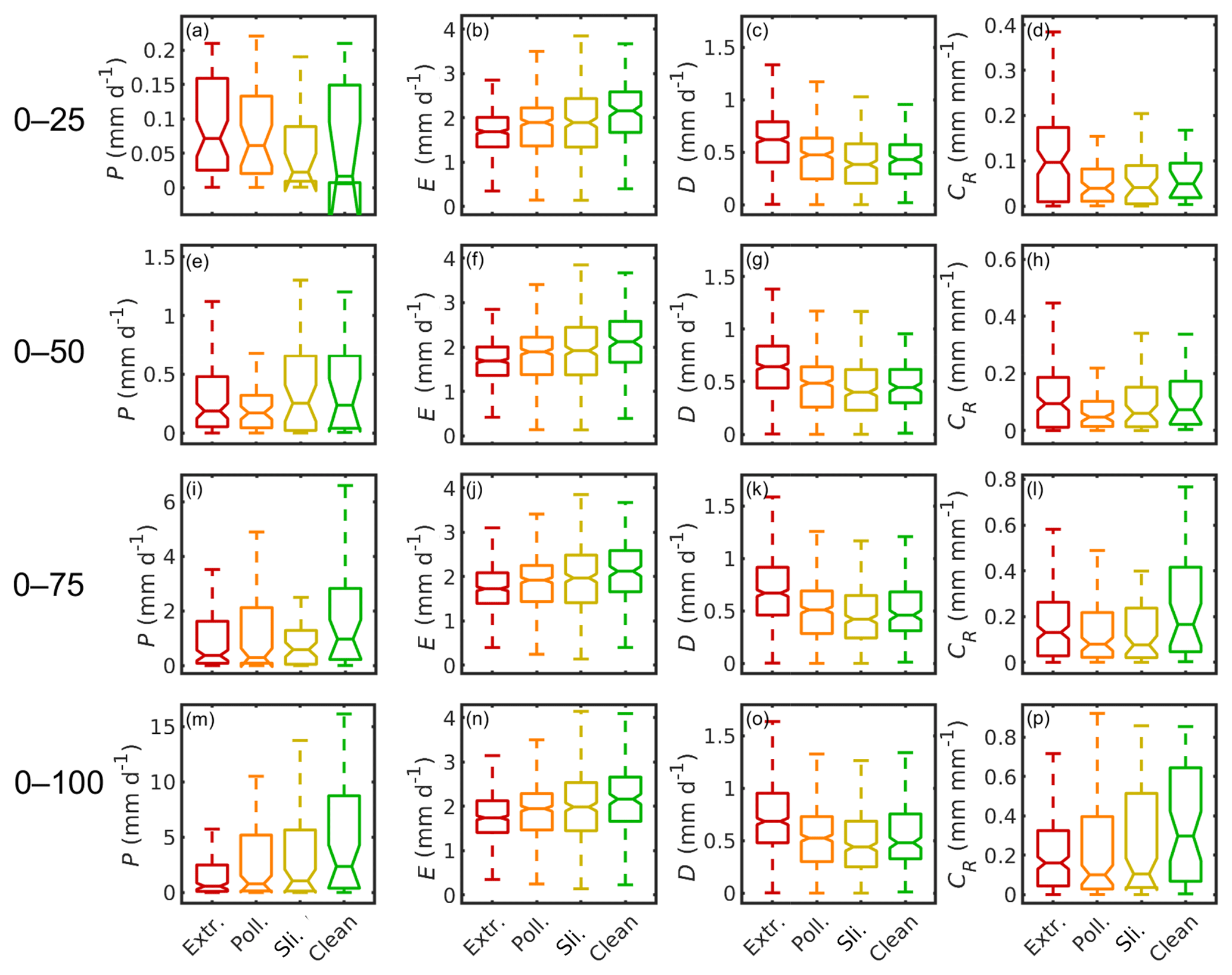
Figure 4Box plots of daily precipitation (P), evapotranspiration (E), drainage (D), and runoff coefficient (CR) stratified by different pollution level (extremely polluted air, polluted air, slightly polluted air, and fairly clean air) and daily precipitation percentiles (rows) from low precipitation (0–25) to all precipitation events (0–100) for 2001–2013. The notches indicate the 95 % confidence levels. Outliers are not shown. The amount of data used for each box is shown in Table 4. See “Statistical methods” for details.
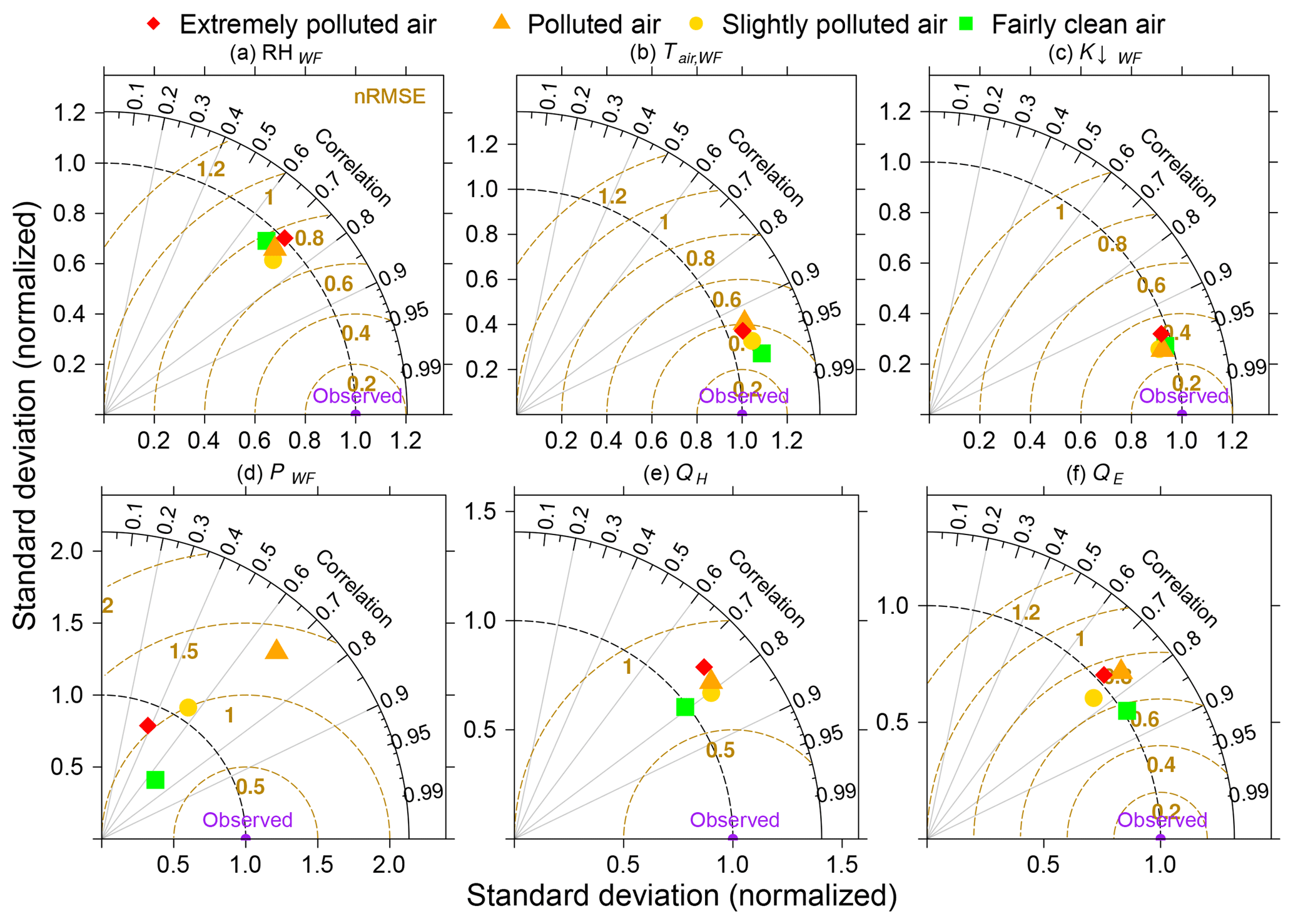
Figure 5Taylor diagram (Taylor, 2001) for hourly (a) relative humidity (RHWF), (b) air temperature (Tair,WF), (c) incoming solar radiation (K↓WF), and daily (d) precipitation (PWF) with corrected WFDEI data assessed with IAP observations stratified by air quality and hourly modelled (e) sensible heat flux (QH) and (f) latent heat flux (QE) against eddy covariance IAP observations from a 47 m height for 2006–2009. The radial axis is normalized standard deviation, the angular axis is the correlation coefficient, and brown dashed lines indicate normalized root mean square error (nRMSE). See “Statistical methods” for details. Note scales differ between plots.
Table 4Number of days of data (N) in each Fig. 4 box plot stratified by pollution level (extremely polluted air, polluted air, slightly polluted air, and fairly clean air) and daily precipitation percentiles (columns) from low precipitation (0–25) to all precipitation events (0–100). See “Statistical methods” for details.

The corrected K↓WF and other meteorological variables correspond well with observations in all air quality levels except for PWF, which still has substantial biases, even after the correction (Fig. 5, Table 3).
3.1.1 Meteorological conditions during haze
Haze events in Beijing typically occur with southerly winds, which bring warm and humid air masses from the south (e.g. Cai et al., 2017; Chen and Wang, 2015; Wu et al., 2017). In addition, the wind speeds are typically slower (<2 m s−1) during haze events (Zheng et al., 2015, 2016). The highly polluted industrial areas are located south of Beijing, so southerly winds transport pollutants from these areas (Zhang et al., 2014; Zhao et al., 2013; Zheng et al., 2015). These meteorological conditions are also favourable for haze formation from local emissions and secondary nucleation (Kulmala et al., 2016; Yao et al., 2018). Due to the wet deposition of aerosols, the high precipitation rates commonly occur on less polluted days (Ouyang et al., 2015).
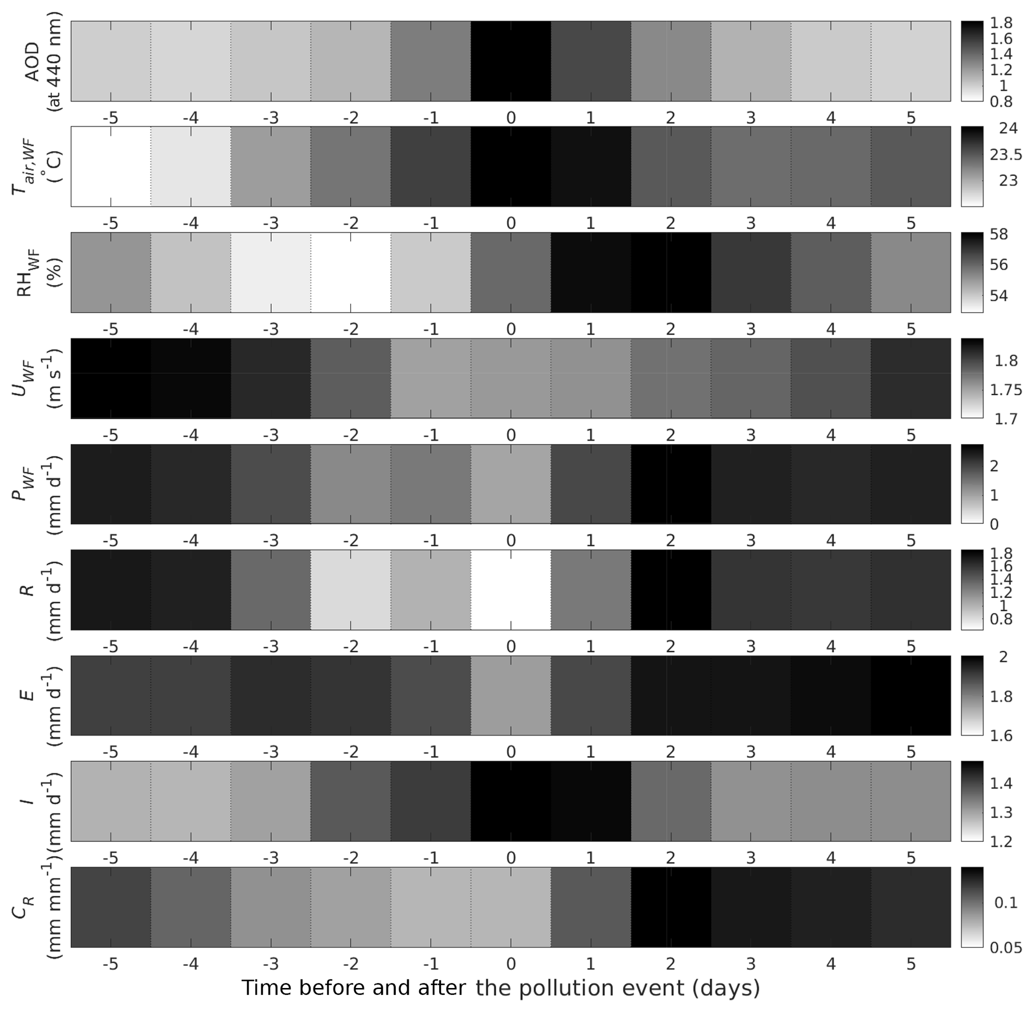
Figure 6Average meteorological conditions of the pollution event days (AOD>1, day 0), 5 d before (days −5 to −1) and 5 d after (days 1 to 5) in 2001–2013. Daily averages (N=568) of aerosol optical depth (AOD), air temperature (Tair,WF), relative humidity (RHWF), and wind speed (UWF) and daily cumulative values of observed precipitation (PWF) and modelled surface runoff (R), evapotranspiration (E), irrigation (I), and the runoff coefficient (CR).
Meteorological conditions during haze events are well represented in the corrected WFDEI dataset. Figure 6 shows the average daily meteorological conditions of all the days when AOD>1 (N=568, day 0), 5 d before and 5 d after for different WFDEI meteorological variables in 2001–2013. When AOD increases in the extremely polluted conditions (from 0.99 on day −5 to 1.82 on day 0), RHWF and Tair,WF also increase (from 55.1 % and 22.5 ∘C on day −5 % to 56.0 % and 24.0 ∘C on day 0), and UWF and PWF decrease (from 1.8 m s−1 and 2.5 mm d−1 on day −5 to 1.8 m s−1 and 1.0 mm d−1 on day 0). The correct description of meteorological conditions during haze events makes the study of water balance during different pollution levels possible using the WFDEI data.
3.2 Evaluation of the SUEWS model in a polluted urban environment
SUEWS model performance is relatively independent of haze levels as its effects on local meteorological conditions are included in the model input variables P, K↓, Tair, and RH. As the incoming longwave radiation (L↓) emitted by the sky is calculated from Tair and RH, which have a positive correlation with the level of pollution in Beijing (e.g. Cai et al., 2017; Chen and Wang, 2015; Wu et al., 2017), the positive correlation of L↓ and air quality is reproduced by SUEWS (Fig. 7b). Therefore, the model performance does not significantly decrease with increasing AOD (Fig. 5, Table 5), even though there are substantial differences in uncertainties of PWF between the different air quality conditions. Surface runoff, which is most sensitive to precipitation, is analysed using normalized values, and therefore the uncertainties in PWF are not crucial to the conclusions.
Table 5Comparison for 2006–2009 of model results with observations, stratified by pollution level (extremely polluted air (AOD>1), polluted air (0.438–1), slightly polluted air (0.203–0.438), and fairly clean air (<0.203)). Data are hourly: sensible heat flux (QH, W m−2) and latent heat flux (QE, W m−2). The superscript “uc” indicates uncorrected variables. See “Statistical methods” for details.
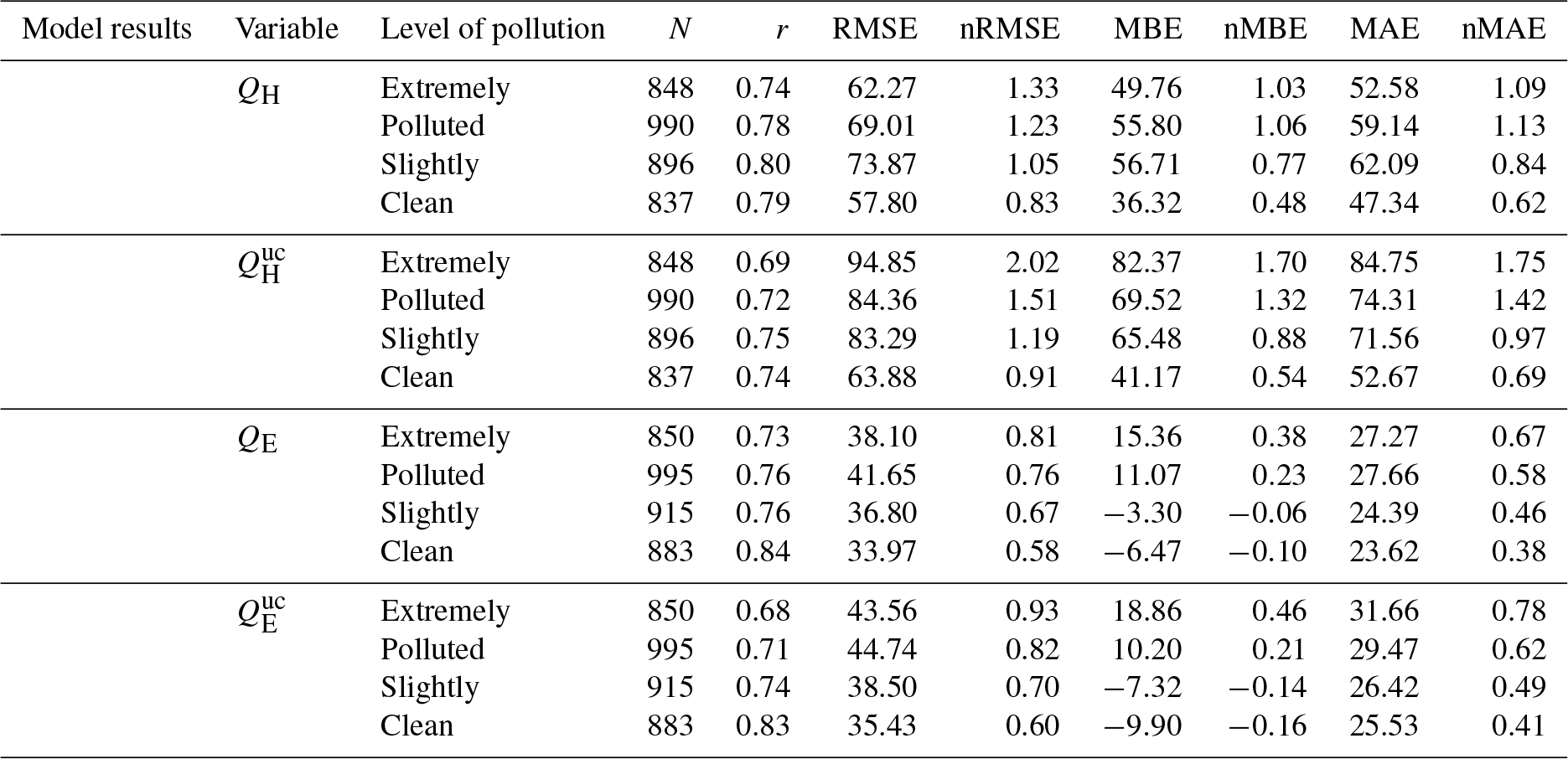
After the above corrections are made to the WFDEI data, the model performance is improved (Table 5) and SUEWS simulates QE well (r>0.73, nRMSE: 0.58 to 0.81 from clean to extremely polluted conditions), and the results during different air quality levels are generally comparable to each other (Fig. 5, Table 5). Also the modelled sensible heat flux (QH) is reasonably good (r>0.74, nRMSE: 0.83 to 1.33 from clean to extremely polluted conditions), overestimating the daytime values slightly. A similar overestimation has been observed with other urban local-scale models used in Beijing (e.g. Liang et al., 2018) and is likely related to the overestimated anthropogenic heat flux (QF) or underestimated storage heat flux (ΔQS) values that cannot be measured easily. Detailed hydrological analysis on the effect of haze can be made using SUEWS forced by WFDEI data in the highly polluted city of Beijing as the performance of the model is similar to the results in the cleaner cities of Vancouver, Los Angeles, London, and Swindon (e.g. Järvi et al., 2011; Kokkonen et al., 2018b; Ward et al., 2016).
3.3 The radiative effect of haze on the surface water balance
Comparison of K↓ for different pollutant levels finds that haze attenuates K↓WF by 167 W m−2 (medians of midday K↓WF of fairly clean conditions and extremely polluted conditions; Fig. 7). This reduces the surface energy availability and sensible heat fluxes (Kajino et al., 2017). In addition, K↓ absorbed by the heavily polluted layer changes the vertical temperature profile, leading to an increased stability, which reduces turbulence and mixing and therefore also the boundary layer height (Petäjä et al., 2016). With less energy available at the surface, evaporation decreases by 0.42 mm d−1 (daily median of fairly clean compared to extremely polluted conditions; Fig. 4). Thus with the same precipitation rate, more water would be stored at the surface or in the soil or directed to surface runoff, especially during the smaller precipitation intensities associated with more polluted levels (Fig. A2). The drainage is decreased by 0.19 mm d−1, and the runoff coefficient (, where I is irrigation) is increased by 0.047 based on the same comparison of daily medians for the 0–25 percentile daily precipitation (Fig. 4). This is because for the most polluted days with the lowest precipitation (0–25 percentiles) P is slightly larger (0.07 mm d−1) and E is the lowest (1.69 mm day−1), resulting in CR being largest (median 0.097), whereas the cleaner conditions are substantially lower (0.039–0.049) (Fig. 4). As higher daily precipitation percentiles are included, the higher amount of P during the fairly clean conditions starts to dominate. Even though the median CR during extremely polluted conditions is higher than during other polluted levels (polluted and slightly polluted conditions) in all of the precipitation classes, CR during fairly clean air starts to be equal to the extreme haze conditions during days with precipitation of 0–75 percentiles (CR: 0.13, 0.08, 0.08, and 0.17 for extremely polluted, polluted, slightly polluted, and fairly clean air, respectively) and exceeds extreme haze conditions when all the percentiles of precipitation are included (0.16, 0.10, 0.10, and 0.30 from extremely polluted to fairly clean conditions).
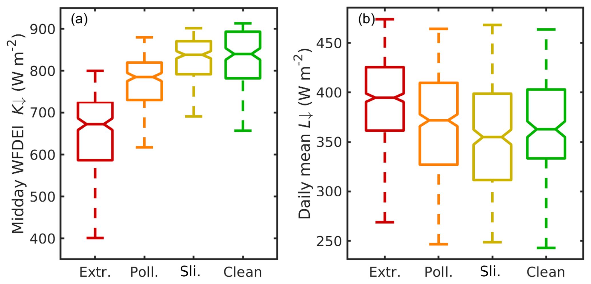
Figure 7Box plots of (a) midday WFDEI incoming solar radiation (K↓WF) and (b) modelled daily mean incoming longwave radiation (L↓) stratified by different pollution level (extremely polluted air, polluted air, slightly polluted, and fairly clean air) for 2001–2013. See “Statistical methods” for details.
Beijing urban top soil is heavily polluted in gardens, on roadsides, and in residential areas (e.g. Chen et al., 2005; Xia et al., 2011). Two-thirds of Beijing's water supply is from groundwater, which is often contaminated by surface pollution sources (Sun et al., 2014). Decreased evaporation with poorer air quality increases surface drainage (0.70, 0.54, 0.44, and 0.50 mm d−1 from extremely polluted to fairly clean conditions) (Fig. 4), potentially causing more infiltration to groundwater from surfaces on occasions when higher atmospheric deposition has occurred and hence potentially making water quality poorer.
The increase in surface runoff during high haze conditions is quite small (Fig. 4) and may not contribute significantly to urban flooding. However, the poorest surface runoff water quality is associated with the first flush of runoff (Deletic and Maksimovic, 1998; Gupta and Saul, 1996; Yufen et al., 2008); thus the days with increased runoff may have poorer water quality. The irrigation of urban green areas might also have a similar effect by flushing the pollutants regularly from the surfaces. The flush of pollutants from contaminated surfaces to urban water bodies as surface runoff from vegetated and impervious surfaces in Beijing has been shown to include significantly more pollutants than rainwater (Yufen et al., 2008). Therefore, the increase in runoff and drainage due to the radiative effect of haze will increase the pollutant loads in already deteriorated urban surface waters (Sun et al., 2014) and groundwater.
In this study the radiative effect of haze on the local-scale hydrological cycle is examined for the period 2001–2013. The hydrological modelling is conducted using Surface Urban Energy and Water Balance Scheme (SUEWS) forced with WATCH WFDEI reanalysis data. The representativeness of WFDEI reanalysis data in a highly polluted urban environment (Beijing) is assessed with meteorological observations from the 325 m IAP tower from a 47 m level. In addition, the SUEWS performance is evaluated against eddy covariance observations of latent and sensible heat fluxes from the same height of the IAP tower. The results are stratified by air quality based on observations of aerosol optical depth (AOD).
The effects of haze are well accounted for in the original WFDEI meteorological variables, except for incoming solar radiation and precipitation. After the correction, daily precipitation totals are generally improved, but there are still substantial differences in the performance between the different air quality levels. After correcting the WFDEI incoming solar radiation with the newly developed haze correction, it compares well to observations across pollution levels (r>0.94, nRMSE<0.33). Evaluation of SUEWS using eddy covariance observations of evaporation in Beijing concludes the model performance is good (r: >0.68 and >0.73; nRMSE: <0.93 and <0.81 using uncorrected and corrected WFDEI forcing data, respectively). Similarly SUEWS performance of the sensible heat flux is rather good (r: >0.69 and >0.74; nRMSE: <2.02 and <1.33 using uncorrected and corrected WFDEI forcing data, respectively). Therefore the local urban water balance can be modelled despite substantial biases in WFDEI precipitation data.
Detailed analyses of water balance terms find that attenuated incoming solar radiation from increased atmospheric aerosol concentrations decreases the daily median evapotranspiration from 2.16 mm d−1 during fairly clean conditions to 1.74 mm d−1 during extremely polluted conditions. This leads to an increased runoff coefficient (from 0.049 to 0.097 during fairly clean and extremely polluted conditions, respectively), especially during smaller precipitation totals (days with precipitation totals in the lower 25th percentile). When all precipitation events are included, the higher precipitation levels during fairly clean conditions induce the highest runoff coefficients (0.30), even though the runoff coefficient during the extremely polluted conditions (0.16) is higher than during other air quality levels (0.10 in both polluted and slightly polluted conditions). Also soil infiltration is increased due to decreased evapotranspiration: drainage from 0.48 mm d−1 during fairly clean conditions to 0.68 mm d−1 during extremely polluted conditions.
This study is the first to examine the radiative effects of haze on the local-scale urban hydrological cycle. The increased surface runoff and soil infiltration are expected to lead to increased pollutant loads washed from polluted surfaces and top layers of soils into urban surface waters and groundwater, which are already poor in the Beijing region. The evaluation of WFDEI reanalysis data gives first results of the representativeness of an reanalysis dataset in a highly polluted urban area. Other reanalysis datasets should also be carefully evaluated and make the necessary corrections prior to use in polluted urban areas.
For the SUEWS manual and software, visit http://suews-docs.readthedocs.io (last access: 6 February 2017; Ward et al., 2017). WATCH WFDEI data can be acquired from ftp://rfdata:forceDATA@ftp.iiasa.ac.at (last access: 17 November 2017; Weedon et al., 2014) and AOD data from https://aeronet.gsfc.nasa.gov/ (last access: 24 July 2018; Holben et al., 1998).
Table A1Notation used in Tables 1 and A2. Details and sources of the values are given in Järvi et al. (2011, 2014).
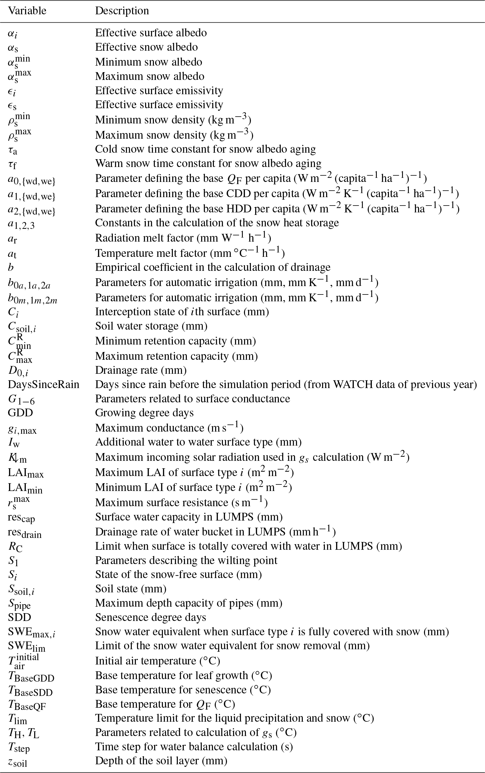
Table A2Model parameters used in SUEWS for different surfaces: buildings (Bldgs), paved (Pav), evergreen vegetation (Everg), deciduous vegetation (Dec), grass, and water. Initial conditions assume there is no snow on the ground, and the leaf area index of each vegetation type is at its minimum value. See Table A1 for notation and Järvi et al. (2011, 2014) for data sources.

Table A3Disaggregation for precipitation parameters (see details from Ward et al., 2017, 2018). Rainfall is evenly distributed among RainAmongN subintervals in a rainy interval for different intensity bins. The number of sub intervals over which to distribute rainfall in each interval is given in MultRainAmongN for three intensity bins. The upper limit for each intensity bin to apply MultRainAmongN is given in MultRainAmongNUpperI.
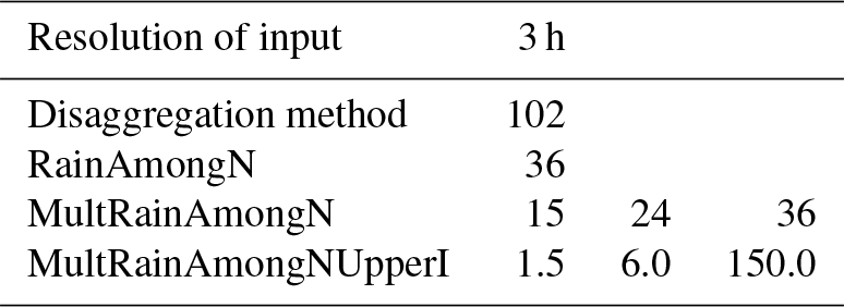
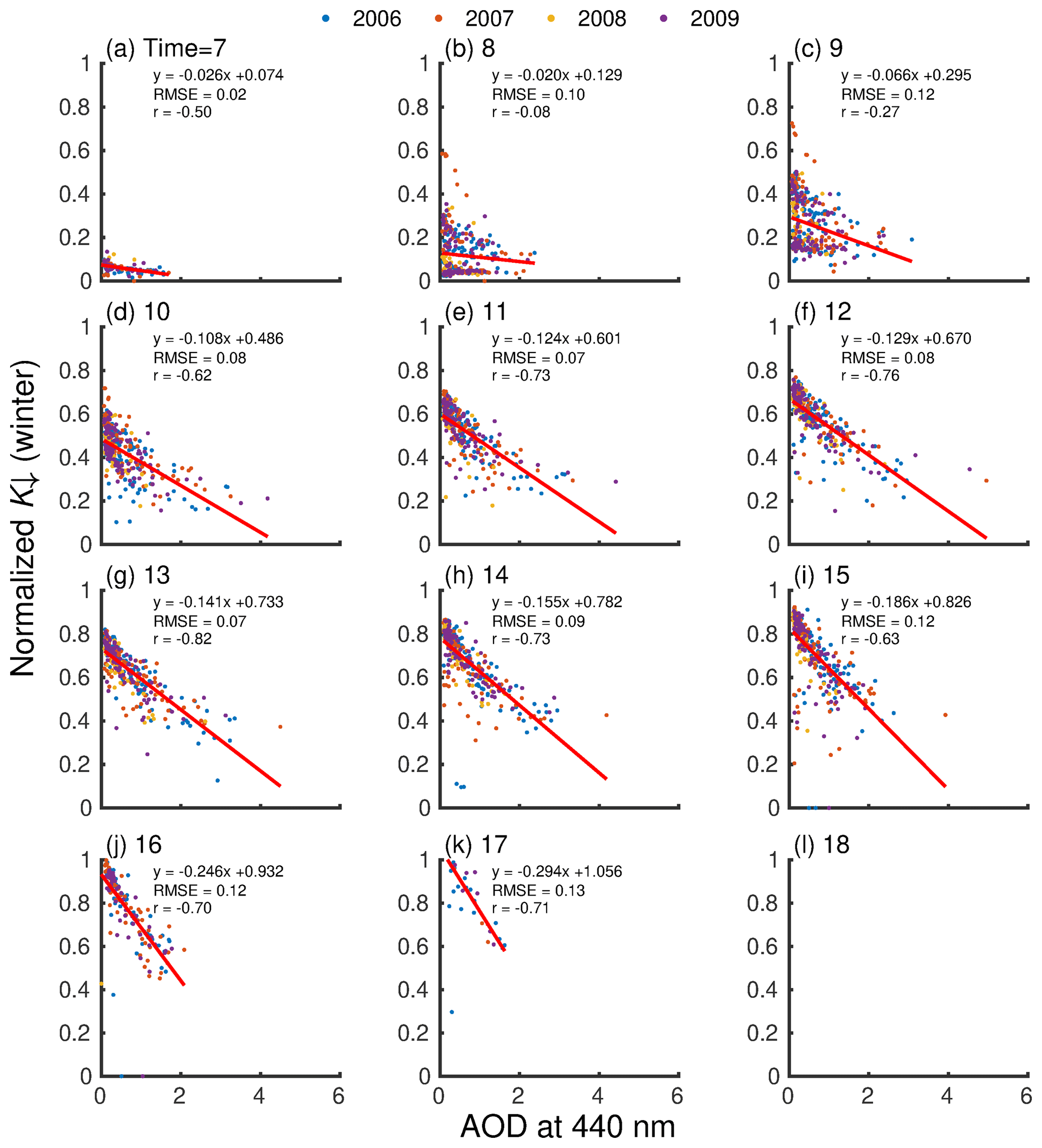
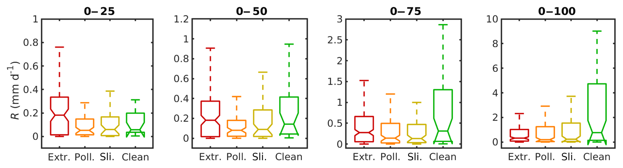
Figure A2Daily cumulative runoff (R) stratified by different pollution level (extremely polluted air, polluted air, slightly polluted air, and fairly clean air) and daily precipitation percentiles from low precipitation (0–25) to all precipitation events (0–100) for 2001–2013. The notches indicate 95 % confidence levels. Outliers are not shown. See “Statistical methods” for details. See also Fig. 4.
TVK and LJ conceived this study; TVK was responsible for the atmospheric and hydrological analyses; SM was responsible for the GIS analysis; HL was responsible for the meteorological measurements. All authors contributed to the writing of the paper.
The authors declare that they have no conflict of interest.
We acknowledge the Beijing Municipality for providing the sites for measurements and Hong-Bin Chen and Philippe Goloub for providing the AOD measurements. The data used are listed in the references.
This research was supported by the Maa- ja vesitekniikan tuki ry (grant no. 36663) and the UK–China Research Innovation Partnership Fund through the Met Office Climate Science for Service Partnership (CSSP) China as part of the Newton Fund (High Res City; AJYG-DX4P1V, Grimmond).
Open access funding provided by Helsinki University Library.
This paper was edited by Joshua Fu and reviewed by two anonymous referees.
Alexander, P. J., Mills, G., and Fealy, R.: Using LCZ data to run an urban energy balance model, Urban Climate, 13, 14–37, https://doi.org/10.1016/j.uclim.2015.05.001, 2015. a, b
Ao, X., Grimmond, C. S. B., Liu, D., Han, Z., Hu, P., Wang, Y., Zhen, X., and Tan, J.: Radiation Fluxes in a Business District of Shanghai, China, J. Appl. Meteorol. Clim., 55, 2451–2468, https://doi.org/10.1175/JAMC-D-16-0082.1, 2016. a
Ao, X., Grimmond, C. S. B., Ward, H. C., Gabey, A. M., Tan, J., Yang, X.-Q., Liu, D., Zhi, X., Liu, H., and Zhang, N.: Evaluation of the Surface Urban Energy and Water Balance Scheme (SUEWS) at a Dense Urban Site in Shanghai: Sensitivity to Anthropogenic Heat and Irrigation, J. Hydrometeorol., 19, 1983–2005, https://doi.org/10.1175/JHM-D-18-0057.1, 2018. a
Beijing Municipal Bureau of Statistics: Beijing statistical yearbook, available at: http://tjj.beijing.gov.cn/English/ (last access: 3 October 2018), 2016. a
Cai, W., Li, K., Liao, H., Wang, H., and Wu, L.: Weather conditions conducive to Beijing severe haze more frequent under climate change, Nat. Clim. Change, 7, 257–263, https://doi.org/10.1038/nclimate3249, 2017. a, b
Che, H., Zhang, X., Chen, H., Damiri, B., Goloub, P., Li, Z., Zhang, X., Wei, Y., Zhou, H., Dong, F., Li, D., and Zhou, T.: Instrument calibration and aerosol optical depth validation of the China Aerosol Remote Sensing Network, J. Geophys. Res.-Atmos., 114, D03206, https://doi.org/10.1029/2008JD011030, 2009. a
Chen, H. and Wang, H.: Haze Days in North China and the associated atmospheric circulations based on daily visibility data from 1960 to 2012, J. Geophys. Res.-Atmos., 120, 5895–5909, https://doi.org/10.1002/2015JD023225, 2015. a, b
Chen, T.-B., Zheng, Y.-M., Lei, M., Huang, Z.-C., Wu, H.-T., Chen, H., Fan, K.-K., Yu, K., Wu, X., and Tian, Q.-Z.: Assessment of heavy metal pollution in surface soils of urban parks in Beijing, China, Chemosphere, 60, 542–551, https://doi.org/10.1016/j.chemosphere.2004.12.072, 2005. a
Cheng, X. L., Liu, X. M., Liu, Y. J., and Hu, F.: Characteristics of CO2 Concentration and Flux in the Beijing Urban Area, J. Geophys. Res.-Atmos., 123, 1785–1801, https://doi.org/10.1002/2017JD027409, 2018. a
Cleveland, W. S.: Robust Locally Weighted Regression and Smoothing Scatterplots, J. Am. Stat. Assoc., 74, 829–836, https://doi.org/10.1080/01621459.1979.10481038, 1979. a
Cleveland, W. S.: LOWESS: A Program for Smoothing Scatterplots by Robust Locally Weighted Regression, Am. Stat., 35, p. 54, https://doi.org/10.2307/2683591, 1981. a
Dee, D. P., Uppala, S. M., Simmons, A. J., Berrisford, P., Poli, P., Kobayashi, S., Andrae, U., Balmaseda, M. A., Balsamo, G., Bauer, P., Bechtold, P., Beljarrs, A. C. M., van de Berg, L., Bidlot, J., Bormann, N., Delsol, C., Dragani, R., Fuentes, M., Geer, A. J., Haimberger, L., Healy, S. B., Hersbach, H., Hólm, E. V., Isaksen, L., Kållberg, P., Köhler, M., Matricardi, M., McNally, A. P., Monge-Sanz, B. M., Morcrette, J.-J., Park, B.-K., Peubey, C., de Rosnay, P., Tavolato, C., Thépaut, J.-N., and Vitart, F.: The ERA-Interim reanalysis: Configuration and performance of the data assimilation system, Q. J. Roy. Meteor. Soc., 137, 553–597, https://doi.org/10.1002/qj.828, 2011. a
Deletic, A. B. and Maksimovic, C. T.: Evaluation of Water Quality Factors in Storm Runoff from Paved Areas, J. Environ. Eng., 124, 869–879, https://doi.org/10.1061/(ASCE)0733-9372(1998)124:9(869), 1998. a
Demuzere, M., Harshan, S., Järvi, L., Roth, M., Grimmond, C. S. B., Masson, V., Oleson, K. W., Velasco, E., and Wouters, H.: Impact of urban canopy models and external parameters on the modelled urban energy balance in a tropical city, Q. J. Roy. Meteor. Soc., 143, 1581–1596, https://doi.org/10.1002/qj.3028, 2017. a
Ding, A. J., Fu, C. B., Yang, X. Q., Sun, J. N., Petäjä, T., Kerminen, V.-M., Wang, T., Xie, Y., Herrmann, E., Zheng, L. F., Nie, W., Liu, Q., Wei, X. L., and Kulmala, M.: Intense atmospheric pollution modifies weather: a case of mixed biomass burning with fossil fuel combustion pollution in eastern China, Atmos. Chem. Phys., 13, 10545–10554, https://doi.org/10.5194/acp-13-10545-2013, 2013. a
Esri: World Imagery – 1 m Imagery, available at: https://www.arcgis.com/home/item.html?id=10df2279f9684e4a9f6a7f08febac2a9 (last access: 31 August 2015), 2009. a
Fu, J., Jiang, D., and Huang, Y.: 1 KM Grid Population Dataset of China, Global Change Research Data Publishing & Repository, https://doi.org/10.3974/geodb.2014.01.06.V1, 2014. a
Grimmond, C. S. B. and Oke, T. R.: An evapotranspiration-interception model for urban areas, Water Resour. Res., 27, 1739–1755, https://doi.org/10.1029/91WR00557, 1991. a, b
Gupta, K. and Saul, A. J.: Specific relationships for the first flush load in combined sewer flows, Water Res., 30, 1244–1252, https://doi.org/10.1016/0043-1354(95)00282-0, 1996. a
HEI International Scientific Oversight Committee: Outdoor Air Pollution and Health in the Developing Countries of Asia: A Comprehensive Review, Special Report 18, Health Effects Institute, Boston, MA, available at: https://www.healtheffects.org/system/files/SR18AsianLiteratureReview.pdf (last access: 9 July 2018), 2010. a
Holben, B., Eck, T., Slutsker, I., Tanré, D., Buis, J., Setzer, A., Vermote, E., Reagan, J., Kaufman, Y., Nakajima, T., Lavenu, F., Jankowiak, I., and Smirnov, A.: AERONET – A Federated Instrument Network and Data Archive for Aerosol Characterization, Remote Sens. Environ., 66, 1–16, https://doi.org/10.1016/S0034-4257(98)00031-5, 1998. a, b, c
Järvi, L., Grimmond, S., and Christen, A.: The Surface Urban Energy and Water Balance Scheme (SUEWS): Evaluation in Los Angeles and Vancouver, J. Hydrol., 411, 219–237, https://doi.org/10.1016/j.jhydrol.2011.10.001, 2011. a, b, c, d, e, f, g, h
Järvi, L., Grimmond, C. S. B., Taka, M., Nordbo, A., Setälä, H., and Strachan, I. B.: Development of the Surface Urban Energy and Water Balance Scheme (SUEWS) for cold climate cities, Geosci. Model Dev., 7, 1691–1711, https://doi.org/10.5194/gmd-7-1691-2014, 2014. a, b, c, d
Järvi, L., Grimmond, C. S. B., McFadden, J. P., Christen, A., Strachan, I. B., Taka, M., Warsta, L., and Heimann, M.: Warming effects on the urban hydrology in cold climate regions, Sci. Rep.-UK, 7, 5833, https://doi.org/10.1038/s41598-017-05733-y, 2017. a
Kajino, M., Ueda, H., Han, Z., Kudo, R., Inomata, Y., and Kaku, H.: Synergy between air pollution and urban meteorological changes through aerosol-radiation-diffusion feedback–A case study of Beijing in January 2013, Atmos. Environ., 171, 98–110, https://doi.org/10.1016/j.atmosenv.2017.10.018, 2017. a
Karsisto, P., Fortelius, C., Demuzere, M., Grimmond, C. S. B., Oleson, K. W., Kouznetsov, R., Masson, V., and Järvi, L.: Seasonal surface urban energy balance and wintertime stability simulated using three land-surface models in the high-latitude city Helsinki, Q. J. Roy. Meteor. Soc., 142, 401–417, https://doi.org/10.1002/qj.2659, 2016. a
Kokkonen, T. V., Grimmond, C. S. B., Christen, A., Oke, T. R., and Järvi, L.: Changes to the Water Balance Over a Century of Urban Development in Two Neighborhoods: Vancouver, Canada, Water Resour. Res., 54, 6625–6642, https://doi.org/10.1029/2017WR022445, 2018a. a
Kokkonen, T. V., Grimmond, C. S. B., Räty, O., Ward, H. C., Christen, A., Oke, T. R., Kotthaus, S., and Järvi, L.: Sensitivity of Surface Urban Energy and Water Balance Scheme (SUEWS) to downscaling of reanalysis forcing data, Urban Climate, 23, 36–52, https://doi.org/10.1016/j.uclim.2017.05.001, 2018b. a, b, c, d, e, f, g, h, i, j, k
Kulmala, M.: Atmospheric chemistry: China's choking cocktail, Nature, 526, 497–499, https://doi.org/10.1038/526497a, 2015. a
Kulmala, M., Petäjä, T., Kerminen, V.-M., Kujansuu, J., Ruuskanen, T., Ding, A., Nie, W., Hu, M., Wang, Z., Wu, Z., Wang, L., and Worsnop, D. R.: On secondary new particle formation in China, Front. Env. Sci. Eng., 10, 8, https://doi.org/10.1007/s11783-016-0850-1, 2016. a
Li, E., Endter-Wada, J., and Li, S.: Characterizing and Contextualizing the Water Challenges of Megacities, J. Am. Water Resour. As., 51, 589–613, https://doi.org/10.1111/1752-1688.12310, 2015. a
Liang, X., Miao, S., Li, J., Bornstein, R., Zhang, X., Gao, Y., Chen, F., Cao, X., Cheng, Z., Clements, C., Dabberdt, W., Ding, A., Ding, D., Dou, J. J., Dou, J. X., Dou, Y., Grimmond, C. S. B., González-Cruz, J. E., He, J., Huang, M., Huang, X., Ju, S., Li, Q., Niyogi, D., Quan, J., Sun, J., Sun, J. Z., Yu, M., Zhang, J., Zhang, Y., Zhao, X., Zheng, Z., and Zhou, M.: SURF: Understanding and Predicting Urban Convection and Haze, B. Am. Meteorol. Soc., 99, 1391–1413, https://doi.org/10.1175/BAMS-D-16-0178.1, 2018. a
Liao, H., Chang, W., and Yang, Y.: Climatic effects of air pollutants over China: A review, Adv. Atmos. Sci., 32, 115–139, https://doi.org/10.1007/s00376-014-0013-x, 2015. a
Liu, H. Z., Feng, J. W., Järvi, L., and Vesala, T.: Four-year (2006–2009) eddy covariance measurements of CO2 flux over an urban area in Beijing, Atmos. Chem. Phys., 12, 7881–7892, https://doi.org/10.5194/acp-12-7881-2012, 2012. a, b, c, d, e
Ma, J. and Liu, Q.: Flora of Beijing: An overview and suggestions for future research, Urban Habitats, 1, 30–44, 2003. a
Menne, M., Durre, I., Korzeniewski, B., McNeal, S., Thomas, K., Yin, X., Anthony, S., Ray, R., Vose, R., Gleason, B. E., and Houston, T.: Global Historical Climatology Network – Daily (GHCN-Daily), Version 3.22, https://doi.org/10.7289/V5D21VHZ, 2012a. a
Menne, M., Durre, I., Vose, R., Gleason, B., and Houston, T.: An overview of the Global Historical Climatology Network-Daily Database, J. Atmos. Ocean. Tech., 29, 897–910, https://doi.org/10.1175/JTECH-D-11-00103.1, 2012b. a
Miao, S., Chen, F., LeMone, M. A., Tewari, M., Li, Q., and Wang, Y.: An Observational and Modeling Study of Characteristics of Urban Heat Island and Boundary Layer Structures in Beijing, J. Appl. Meteorol. Clim., 48, 484–501, https://doi.org/10.1175/2008JAMC1909.1, 2009. a
Miao, S., Dou, J., Chen, F., Li, J., and Li, A.: Analysis of observations on the urban surface energy balance in Beijing, Sci. China Earth Sci., 55, 1881–1890, https://doi.org/10.1007/s11430-012-4411-6, 2012. a, b
Monteith, J. L.: Evaporation and the environment, Symp. Soc. Exp. Biol., 19, 205–234, 1965. a
Murto, S.: The impact of aerosols on the sensible and latent heat fluxes in Beijing, Master's thesis, University of Helsinki, available at: http://urn.fi/URN:NBN:fi-fe2017112252520 (last access: 3 October 2018), 2017. a
OpenStreetMap contributors: Maps of Beijing area, available at: https://planet.osm.org, https://www.openstreetmap.org (last access: 18 September 2018), 2015. a
Ouyang, W., Guo, B., Cai, G., Li, Q., Han, S., Liu, B., and Liu, X.: The washing effect of precipitation on particulate matter and the pollution dynamics of rainwater in downtown Beijing, Sci. Total Environ., 505, 306–314, https://doi.org/10.1016/j.scitotenv.2014.09.062, 2015. a
Penman, H. L.: Natural evaporation from open water, bare soil and grass, P. Roy. Soc. Lond. A Mat., 193, 120–145, https://doi.org/10.1098/rspa.1948.0037, 1948. a
Petäjä, T., Järvi, L., Kerminen, V.-M., Ding, A., Sun, J., Nie, W., Kujansuu, J., Virkkula, A., Yang, X., Fu, C., Zilitinkevich, S., and Kulmala, M.: Enhanced air pollution via aerosol-boundary layer feedback in China, Sci. Rep.-UK, 6, 18998, https://doi.org/10.1038/srep18998, 2016. a, b, c, d
Rodriguez, F., Andrieu, H., and Creutin, J.-D.: Surface runoff in urban catchment: morphological identification of unit hydrographs from urban databanks, J. Hydrol., 283, 146–168, https://doi.org/10.1016/S0022-1694(03)00246-4, 2003. a
Shao, M., Tang, X., Zhang, Y., and Li, W.: City clusters in China: air and surface water pollution, Front. Ecol. Environ., 4, 353–361, https://doi.org/10.1890/1540-9295(2006)004[0353:CCICAA]2.0.CO;2, 2006. a
Stewart, I. D. and Oke, T. R.: Local climate zones for urban temperature studies, B. Am. Meteorol. Soc., 93, 1879–1900, https://doi.org/10.1175/BAMS-D-11-00019.1, 2012. a
Sun, F., Yang, Z., and Huang, Z.: Challenges and Solutions of Urban Hydrology in Beijing, Water Resour. Manag., 28, 3377–3389, https://doi.org/10.1007/s11269-014-0697-9, 2014. a, b, c, d
Tang, G., Zhang, J., Zhu, X., Song, T., Münkel, C., Hu, B., Schäfer, K., Liu, Z., Zhang, J., Wang, L., Xin, J., Suppan, P., and Wang, Y.: Mixing layer height and its implications for air pollution over Beijing, China, Atmos. Chem. Phys., 16, 2459–2475, https://doi.org/10.5194/acp-16-2459-2016, 2016. a
Taylor, K. E.: Summarizing multiple aspects of model performance in a single diagram, J. Geophys. Res.-Atmos., 106, 7183–7192, https://doi.org/10.1029/2000JD900719, 2001. a, b
Wang, J., Wang, S., Jiang, J., Ding, A., Zheng, M., Zhao, B., Wong, D. C., Zhou, W., Zheng, G., Wang, L., Pleim, J. E., and Hao, J.: Impact of aerosol-meteorology interactions on fine particle pollution during China's severe haze episode in January 2013, Environ. Res. Lett., 9, 094002, https://doi.org/10.1088/1748-9326/9/9/094002, 2014. a
Ward, H. and Grimmond, C.: Assessing the impact of changes in surface cover, human behaviour and climate on energy partitioning across Greater London, Landscape Urban Plan., 165, 142–161, https://doi.org/10.1016/j.landurbplan.2017.04.001, 2017. a
Ward, H. C., Kotthaus, S., Järvi, L., and Grimmond, C. S. B.: Surface Urban Energy and Water Balance Scheme (SUEWS): development and evaluation at two UK sites, Urban Climate, 18, 1–32, https://doi.org/10.1016/j.uclim.2016.05.001, 2016. a, b, c
Ward, H. C., Järvi, L., Onomura, S., Lindberg, F., Olofson, F., Gabey, A., and Grimmond, C. S. B.: SUEWS Manual V2017b, available at: http://suews-docs.readthedocs.io (last access: 6 February 2017), 2017. a, b, c, d, e
Ward, H. C., Tan, Y. S., Gabey, A. M., Kotthaus, S., and Grimmond, C. S. B.: Impact of temporal resolution of precipitation forcing data on modelled urban-atmosphere exchanges and surface conditions, Int. J. Climatol., 36, 649–662, https://doi.org/10.1002/joc.5200, 2018. a, b, c, d
Weedon, G. P., Gomes, S., Viterbo, P., Österle, H., Adam, J. C., Bellouin, N., Boucher, O., and Best, M.: The WATCH Forcing Data 1958–2001: a meteorological forcing dataset for land surface- and hydrological models, WATCH Technical Report 22, available at: http://www.eu-watch.org/publications/technical-reports (last access: 25 November 2015), 2010. a
Weedon, G. P., Balsamo, G., Bellouin, N., Gomes, S., Best, M., and Viterbo, P.: The WFDEI meteorological forcing data set: WATCH Forcing Data methodology applied to ERA-Interim reanalysis data, Water Resour. Res., 50, 7505–7514, https://doi.org/10.1002/2014WR015638, 2014. a, b, c, d
Wu, P., Ding, Y., and Liu, Y.: Atmospheric Circulation and Dynamic Mechanism for Persistent Haze Events in the Beijing-Tianjin-Hebei Region, Adv. Atmos. Sci., 34, 429–440, https://doi.org/10.1007/s00376-016-6158-z, 2017. a, b
Xia, X., Chen, X., Liu, R., and Liu, H.: Heavy metals in urban soils with various types of land use in Beijing, China, J. Hazard. Mater., 186, 2043–2050, https://doi.org/10.1016/j.jhazmat.2010.12.104, 2011. a, b
Yao, L., Garmash, O., Bianchi, F., Zheng, J., Yan, C., Kontkanen, J., Junninen, H., Mazon, S. B., Ehn, M., Paasonen, P., Sipilä, M., Wang, M., Wang, X., Xiao, S., Chen, H., Lu, Y., Zhang, B., Wang, D., Fu, Q., Geng, F., Li, L., Wang, H., Qiao, L., Yang, X., Chen, J., Kerminen, V.-M., Petäjä, T., Worsnop, D. R., Kulmala, M., and Wang, L.: Atmospheric new particle formation from sulfuric acid and amines in a Chinese megacity, Science, 361, 278–281, https://doi.org/10.1126/science.aao4839, 2018. a
Yufen, R., Xiaoke, W., Zhiyun, O., Hua, Z., Xiaonan, D., and Hong, M.: Stormwater Runoff Quality from Different Surfaces in an Urban Catchment in Beijing, China, Water Environ. Res., 80, 719–724, https://doi.org/10.2175/106143008X276660, 2008. a, b
Zhang, R. H., Li, Q., and Zhang, R. N.: Meteorological conditions for the persistent severe fog and haze event over eastern China in January 2013, Sci. China Earth Sci., 57, 26–35, https://doi.org/10.1007/s11430-013-4774-3, 2014. a
Zhao, X. J., Zhao, P. S., Xu, J., Meng,, W., Pu, W. W., Dong, F., He, D., and Shi, Q. F.: Analysis of a winter regional haze event and its formation mechanism in the North China Plain, Atmos. Chem. Phys., 13, 5685–5696, https://doi.org/10.5194/acp-13-5685-2013, 2013. a
Zheng, G., Duan, F., Ma, Y., Zhang, Q., Huang, T., Kimoto, T., Cheng, Y., Su, H., and He, K.: Episode-Based Evolution Pattern Analysis of Haze Pollution: Method Development and Results from Beijing, China, Environ. Sci. Technol., 50, 4632–4641, https://doi.org/10.1021/acs.est.5b05593, 2016. a
Zheng, G. J., Duan, F. K., Su, H., Ma, Y. L., Cheng, Y., Zheng, B., Zhang, Q., Huang, T., Kimoto, T., Chang, D., Pöschl, U., Cheng, Y. F., and He, K. B.: Exploring the severe winter haze in Beijing: the impact of synoptic weather, regional transport and heterogeneous reactions, Atmos. Chem. Phys., 15, 2969–2983, https://doi.org/10.5194/acp-15-2969-2015, 2015. a, b