the Creative Commons Attribution 4.0 License.
the Creative Commons Attribution 4.0 License.
 | 24 May 2019
Influence of ENSO and MJO on the zonal structure of tropical tropopause inversion layer using high-resolution temperature profiles retrieved from COSMIC GPS Radio Occultation
Toshitaka Tsuda
Masatomo Fujiwara
Using COSMIC GPS Radio Occultation (RO) observations from January 2007 to December 2016, we retrieved temperature profiles with the height resolution of about 0.1 km in the upper troposphere and lower stratosphere (UTLS). We investigated the distribution of static stability (N2) and the zonal structure of the tropopause inversion layer (TIL) in the tropics, where a large change in the temperature gradient occurs associated with sharp variations in N2. We show the variations in the mean N2 profiles in coordinates relative to the cold-point tropopause (CPT). A very thin (<1 km) layer is found with average maximum N2 in the range of 11.0– s−2. The mean and standard deviation of TIL sharpness, defined as the difference between the maximum N2 (maxN2) and minimum N2 (minN2) within ±1 km of the CPT, is s−2. The maxN2 is typically located within 0.5 km above CPT.
We focused on the variation in TIL sharpness in two longitude regions, 90–150∘ E (Maritime Continent; MC) and 170–230∘ E (Pacific Ocean; PO), with different land–sea distribution. Seasonal variations in TIL sharpness and thickness were related to the deep convective activity represented by low outgoing longwave radiation (OLR) during the Australian and Asian monsoons. The deviation from the mean sharpness (sharpness anomaly) was out of phase with the OLR anomaly in both the MC and PO. The correlation between the sharpness anomaly over the MC and PO and the sea surface temperature (SST) Niño 3.4 index was −0.66 and +0.88, respectively. During La Niña (SST Niño 3.4 K) in the MC and El Niño (SST Niño 3.4 K) in the PO, warmer SSTs in the MC and PO produce more active deep convection that tends to force the air upward to the tropopause layer and increase the temperature gradient there. The intraseasonal variation in sharpness anomaly during slow and fast episodes of the Madden–Julian Oscillation (MJO) demonstrates that eastward propagation of the positive sharpness anomaly is associated with organized deep convection. Deep convection during MJO will tend to decrease N2 below CPT and increase N2 above CPT, thus enlarging the TIL sharpness. Convective activity in the tropics is a major control on variations in tropopause sharpness at intraseasonal to interannual timescales.
- Article
(8836 KB) - Full-text XML
- BibTeX
- EndNote


The tropical tropopause layer (TTL) at a height of 12–19 km plays an important role in the Earth's climate, as tropospheric air enters the stratosphere mainly in this region, where stratosphere–troposphere exchange (STE) processes occur (Holton et al., 1995). The dynamics and radiative processes in the TTL have received much attention in the decades since the first observation of a slow meridional circulation, the Brewer–Dobson circulation (e.g., Butchart, 2014). In the tropics, the tropopause is defined as either the lapse rate tropopause (LRT) or the cold-point tropopause (CPT). Here, the LRT refers to “the lowest level where the temperature lapse rate decreases to 2 K/km provided the average between this and higher levels within 2 km does not exceed 2 K/km” (World Meteorological Organization; WMO, 1957), while the CPT is the level of the minimum temperature.
The tropopause inversion layer (TIL) is a narrow layer about 1–2 km from the CPT that is characterized by a sharp change in the vertical gradient of the temperature profile, which is also recognized in the static stability profile (Grise et al., 2010; Bell and Geller, 2008; Birner, 2006; Birner et al., 2002). Using routine radiosonde sounding data, a strong mean inversion at the tropopause in the midlatitudes was analyzed (Birner et al., 2002; Birner, 2006). Grise et al. (2010) conducted a global survey of the TIL characteristics, including annual cycle, horizontal distribution, and interannual variations related to the stratospheric Quasi-Biennial Oscillation (QBO) using the Global Positioning System Radio Occultation (GPS-RO) data. TIL is a boundary within the TTL that controls the mixing of air between the troposphere and stratosphere (e.g., Fujiwara and Takahashi, 2001). A very low temperature in the TTL causes dehydration of the air entering the stratosphere (Mote et al., 1996; Fueglistaler et al., 2009).
The static stability is expressed as the square of the Brunt–Väisälä or buoyancy frequency (N2). N2 is the main factor in the dispersion relations for atmospheric waves, including medium-scale gravity waves and planetary-scale equatorial waves such as Kelvin waves and mixed Rossby–gravity waves (Andrews et al., 1987). Birner (2006) found that the mean N2 shows enhanced values near the extratropical tropopause compared to the extratropical lower stratospheric values. Furthermore, Grise et al. (2010) found the largest magnitudes of N2 between 10 and 15∘ latitude in both hemispheres during the Northern Hemisphere (NH) winter season. The spectrum of normalized temperature fluctuations associated with gravity waves is sensitive to changes in N2 (Smith et al., 1987; Fritts et al., 1988). Therefore, an accurate understanding of its horizontal distribution and temporal variations, particularly in the tropics, is important when investigating the characteristics of atmospheric wave propagation. The 20 d Kelvin wave propagation influences the structure of the tropopause height and the value of N2 (Randel and Wu, 2005; Tsuda et al., 1994).
Randel and Wu (2005) demonstrated eastward phase tilt with the height of Kelvin waves that modulate the climatological cold tropopause over Indonesia with the maximum amplitude near the tropical tropopause (∼17 km). A long-term analysis using Singapore radiosonde data and GPS-RO results showed that Kelvin wave activity was stronger during the transition from the easterly to westerly phase of the QBO (Shiotani and Horinouchi, 1993; Randel et al., 2003; Venkat Ratnam et al., 2006). The El Niño and La Niña events, known as the El Niño Southern Oscillation (ENSO), considerably influence the equatorial wave activity and the TTL (Trenberth, 1997; Nishimoto and Shiotani, 2012; Scherllin-Pirscher et al., 2012). The intraseasonal variation in the tropics, known as the Madden–Julian Oscillation (MJO), tends to be more active toward the eastern Pacific during El Niño events (Son et al., 2017). The static stability in the upper troposphere tends to decrease with the deep convection associated with the MJO (Nishimoto and Yoden, 2017).
Holloway and Neelin (2007) found negative correlation of temperature perturbations between the free troposphere (about 800–200 hPa) and the convective cold top (about 100–50 hPa). The cooling in the convective cold top is due to a hydrostatic adjustment to the deep convective heating (Holloway and Neelin, 2007). Paulik and Birner (2012) identified typical temperature perturbations in the deep convective cloud associated with reduced ozone events, a warm anomaly in the middle and upper troposphere and a cold anomaly in the TTL. We are also interested in the characteristics of static stability in the TTL associated with the convective activity.
The sharp increase in N2 across the tropopause (i.e., the sharpness) and the thickness of the layer of maximum N2 above the tropopause (i.e., between 80 % reaching to and decreasing from maximum N2) have been determined in previous studies (Bell and Geller, 2008; Kim and Son, 2012) using both ground- and satellite-based observations (we describe this definition in Fig. 2b). For example, Bell and Geller (2008) analyzed the twice-daily standard radiosonde data from WMO stations and found that the thickness was ∼1 km at low latitudes. Using data from the CHAllenging Mini satellite Payload (CHAMP) GPS-RO mission (Wickert et al., 2001), Schmidt et al. (2005) reported that the tropopause sharpness varies less throughout the year in the tropics than in polar regions. Ratnam et al. (2005), also using the CHAMP dataset, reported an association between greater sharpness and a higher and colder tropopause.
Since the launch of Constellation Observing System for Meteorology Ionosphere and Climate (COSMIC) GPS-RO in April 2006 (Anthes et al., 2008), which has a much greater number of occultations than CHAMP, investigation of the global characteristics of the tropical tropopause has intensified (e.g., Grise et al., 2010; Son et al., 2011; Kim and Son, 2012). The tropopause sharpness is defined as the difference between the mean N2 () in the region up to 1 km above the LRT or CPT (), and in the region down to 1 km below the LRT or CPT () (Kim and Son, 2012; Son et al., 2011). Son et al. (2011) showed maximum sharpness over the western Pacific region in all seasons with slightly higher values during NH winter, while Kim and Son (2012) reported that the local structure and seasonal variability of the tropopause sharpness are associated with convectively coupled equatorial waves. Averaging the N2 profile within ±1 km of the LRT or CPT can reduce fluctuations caused by small-scale perturbations. Pilch Kedzierski et al. (2016) described the role of MJO, QBO, Kelvin, inertia–gravity, and Rossby waves in modulating the maximum N2 (maxN2) above the LRT in the tropics using the long-term COSMIC dataset.
Fine-scale temperature profiles (T) from GPS-RO measurements commonly have ∼1 km vertical resolution in the upper troposphere and lower stratosphere (UTLS) (Kursinski et al., 1997). The actual effective vertical resolution of RO measurements increases in the region of increased refractive gradients such as inversion layers above the boundary layer or the tropopause. Support from the COSMIC Data Analysis and Archive Center (CDAAC) allowed us to retrieve the dry temperature from COSMIC with higher resolution, reaching 0.1 km, in the UTLS (Noersomadi and Tsuda, 2017). We are motivated to utilize the long-term COSMIC GPS-RO data at a vertical resolution of 0.1 km to investigate the annual, interannual, and intraseasonal variability in properties of the tropical tropopause, i.e., the static stability and TIL parameters (sharpness and thickness). We begin by describing the latitudinal and longitudinal distributions of N2 relative to CPT height. After displaying N2 distributions in the tropics, we investigate the relationships between TIL and ENSO variability, and between TIL and MJO activity.
We briefly explain the difference between dry temperature from two COSMIC datasets, cosmicfsi and cosmic2013, and their comparison with radiosonde data. We use cosmic2013 data only from October 2011 to March 2012 (183 d), the duration of the international collaborative campaign called the cooperative Indian Ocean experiment on intraseasonal variability in the year 2011 and the joint project of Dynamics of the Madden–Julian Oscillation (CINDY-DYNAMO 2011) (Yoneyama et al., 2013; Zhang et al., 2013). For the long-term analysis, we utilize cosmicfsi from 2007 to 2016 (10 years) to derive N2 and determine the TIL parameters relative to the CPT. In the following, we outline details of high-resolution T profiles, TIL definitions, and supporting information.
2.1 High-resolution temperature profiles of COSMIC GPS-RO
The GPS limb soundings received by low-Earth-orbit satellites that pass through the lower stratosphere down to the troposphere may contain multipath atmospheric signals, such as atmospheric minor constituents and sharp gradients at the tropopause (Melbourne, 2004). COSMIC GPS-RO provides 1500–2000 profiles d−1 (∼400 profiles over 10∘ S–10∘ N) (Anthes, 2011). Nevertheless, the number of profiles decreased significantly in 2015 and 2016 (60–100 profiles over 10∘ S–10∘ N). The COSMIC retrievals apply wave optics algorithms such as full spectrum inversion (FSI) and phase matching (PM) (Jensen et al., 2003, 2004), transforming the entire phase and amplitude of the occultation signal to derive the dry atmospheric temperature profiles preserving vertical resolution of ∼0.1 km at lower altitudes (Anthes, 2011; Gorbunov, 2002).
The cosmicfsi datasets use FSI up to 30 km altitude, but reliable T profiles representing small perturbations in the lower stratosphere due to atmospheric gravity waves are limited to below ∼28 km due to increasing noise from the retrieval data processing (Tsuda et al., 2011). At altitudes above 30 km, T of cosmicfsi is obtained from the time derivative of the excess phase of the GPS signal (the geometrical optic method; Kursinski et al., 1997), which was used above 20 km for COSMIC data re-processed by CDAAC (cosmic2013). The cosmic2013 dataset was retrieved using PM and smoothed over a 0.5 km scale in the range 10–20 km (Sokolovskiy et al., 2014; Zeng et al., 2016). There was good agreement between the T profiles in the UTLS for both COSMIC datasets and radiosonde data, and the mean difference of CPT temperatures was within ±0.4 K (Noersomadi and Tsuda, 2017). The discrepancy in the CPT altitude between cosmicfsi and the campaign radiosonde dataset was 70 m (mean) and 100 m (median) (Noersomadi and Tsuda, 2017). The cosmicfsi dataset is freely available on the Inter-university Upper atmosphere Global Observation NETwork (IUGONET) system of the metadata database of the Japanese inter-university research program (Hayashi et al., 2013).
We found 2312 and 3387 occultation profiles (∼12 and ∼18 profiles d−1) in cosmicfsi and cosmic2013, respectively, inside 10∘ S–10∘ N, 90–150∘ E (the Maritime Continent region) within a 183 d period in 2011–2012. The difference in the total number of occultations between the two retrievals is possibly caused by a different algorithm and background extrapolation model for bending angles as reported by Noersomadi and Tsuda (2017). Discussion of the difference between the retrieval algorithm for cosmicfsi and for cosmic2013 is beyond the scope of this study. To compare the shape of N2 profiles derived from T by cosmicfsi and cosmic2013 that have different vertical resolution, we use radiosonde observations collected during the CINDY-DYNAMO 2011 campaign. Table 1 lists the 13 stations in the Maritime Continent where approximately twice-daily routine balloon soundings with 2 s recording were conducted. The total number of radiosonde balloons successfully lifted up to >2 km above the CPT is 3996 (∼21 profiles d−1).
Table 1Radiosonde stations for daily routine balloon launches during the CINDY-DYNAMO 2011 campaign around the Maritime Continent. All stations apart from no. 2 are in Indonesia. The “Number of profiles” column lists the number of successful balloon soundings that reached >2 km above the CPT.

We adjusted T from GPS-RO in the geometrical height domain to the geopotential height used for radiosonde data before performing the comparison. Figure 1 shows a typical COSMIC profile on 24 November 2011 at 12:43 UT, which is located within ∼115 km horizontal radius from the balloon observation launched at 11:35 UT at Surabaya station (7.37∘ S, 112.78∘ E). Assuming the average ascent rate of the balloon is ∼5 m s−1 (Gong and Geller, 2010), the temperature measurement at 18 km occurred at around 12:35 UT, so the actual time difference with the occultation event is less than 30 min in the UTLS. The T from cosmicfsi agrees very well with the radiosonde result, particularly above 16.5 km. The cosmicfsi shows small-scale perturbations and large N2 above the CPT, as shown in the radiosonde data.
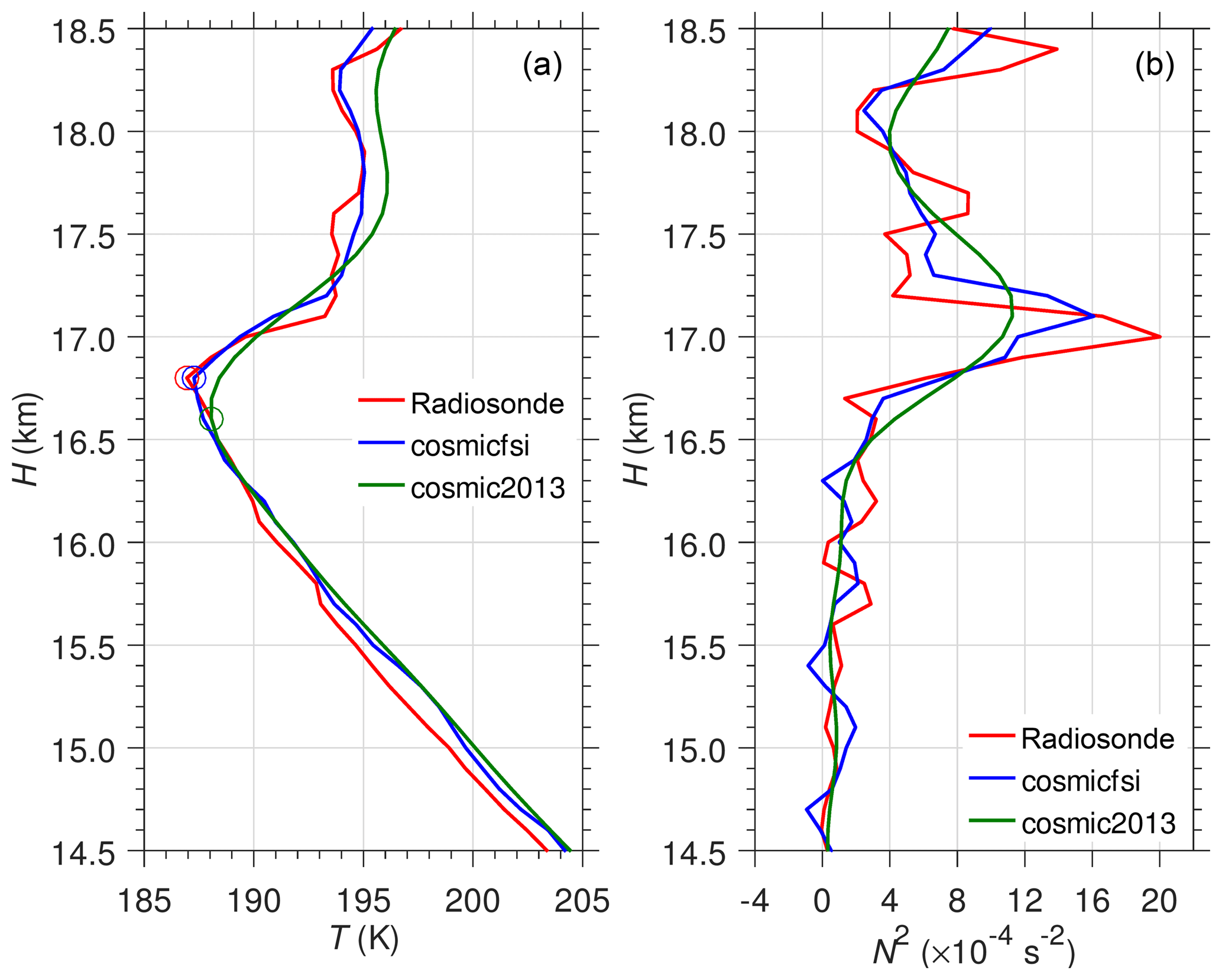
Figure 1A typical COSMIC GPS-RO profile near the radiosonde balloon launch in Surabaya on 24 November 2011. Circles in panel (a) indicate the CPT.
The mean N2 profiles of all available cosmicfsi, cosmic2013, and radiosonde data within the 183 d period are shown in Fig. 2a. The N2 profile just above the CPT from cosmicfsi that agreed very well with the radiosonde data is sharper than the N2 from cosmic2013. Figure 2b shows the zonal mean of N2 over 10∘ S–10∘ N latitude throughout the 10 years of cosmicfsi data (329 396 profiles). The existence of a sharp thin layer is seen from the long-term cosmicfsi dataset. This study mainly discusses the sharpness (S-ab, where “ab” means “above and below” the CPT) and thickness (dH), which are defined in Fig. 2b.

Figure 2Mean N2 profiles from radiosonde (red), cosmicfsi (blue), and cosmic2013 (green) data during CINDY-DYNAMO 2011 (a). Zonal mean N2 profile in the 10∘ S–10∘ N latitude range from 10 years of cosmicfsi data (b). All heights are relative to the CPT.
2.2 TIL definitions
There are several definitions of TIL related to N2 behavior analyzed with GPS-RO data. Grise et al. (2010) showed minor differences in the zonal mean N2 profile relative to LRT and CPT in the tropics. Randel et al. (2007) and Wang et al. (2013) investigate TIL using temperature gradients. Schmidt et al. (2005) and Son et al. (2011) defined the TIL with respect to LRT height; more recently, Gettelman and Wang (2015) and Pilch Kedzierski et al. (2016) used the definition with respect to LRT height. Ratnam et al. (2005) and Kim and Son (2012) defined the tropopause sharpness as the change in the temperature gradient across the CPT. Considering that CPT is the appropriate reference for the tropical tropopause (Kim and Alexander, 2015), we define TIL parameters relative to CPT height in this study.
We obtain TIL parameters from the individual N2 profiles, limiting the height range to ±3 km relative to the CPT, where most of the maximum and minimum peaks of N2 are located. Definitions of the TIL parameters are summarized in Table 2. We define TIL sharpness as follows:
-
S-aCPT is the difference between and N2 at the CPT,
-
S-bCPT represents the difference between N2 at the CPT and minimum (), and
-
S−ab represents the difference between and (i.e., S-ab is equal to the sum of S-aCPT and S-bCPT).
The TIL thickness definitions include the following:
-
dH-aCPT and dH-bCPT are the corresponding distances of and relative to the CPT, respectively;
-
dH-ab is the distance between height of and height of ; and
-
dH is the thickness over which N2≥80 % of maxN2.
We will focus on seasonal variation in S-ab and dH in Sect. 3.3. We have analyzed how the results change quantitatively when using the difference between and , instead of averaging along ±1 km relative to CPT as was done by Kim and Son (2012), with an effectively higher vertical-resolution dataset. In order to obtain dH we need to define the corresponding N2 value. Considering the stable N2 value in the lower stratosphere s−2 and the maxN2 s−2 (Fig. 2b), the threshold of N2 should be larger than 65 % of maxN2. We choose 80 % as the threshold.
Table 2Definitions of TIL sharpness and thickness.
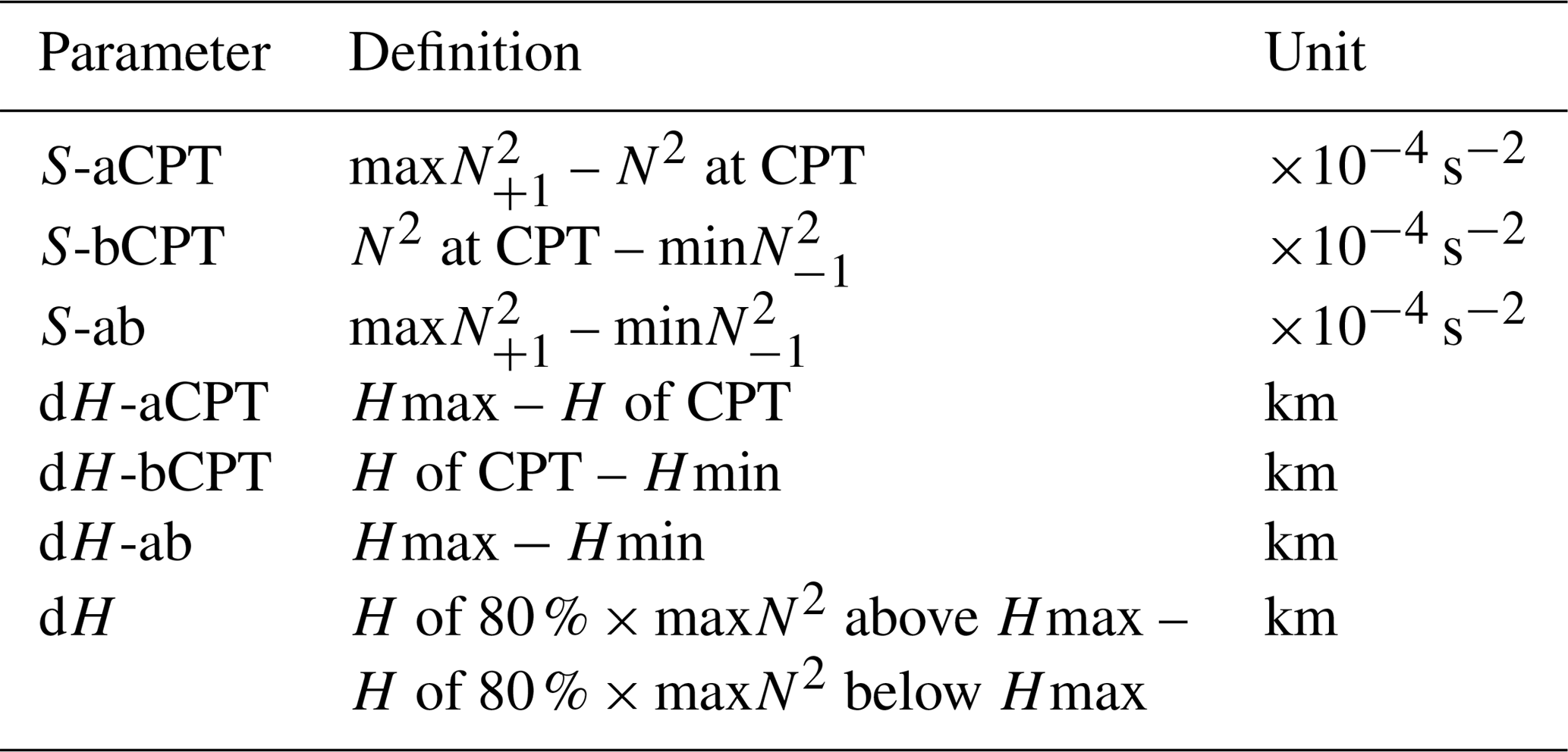
Hmax: H of . Hmin: H of . Subscript ±1 indicates within ±1 km.
The TIL parameters are sorted on a longitude and latitude grid. The grid cells with no available TIL data are denoted as missing values. We analyze the frequency distribution and the climatology of TIL parameters in the region 30∘ S–30∘ N, 0–360∘ E in the next section. To investigate the interannual and intraseasonal variations, we focus on the low latitudes, 10∘ S–10∘ N. Due to the limited number of COSMIC profiles in each grid cell (1 or 2), we then averaged 5 d for data for each grid cell recursively using a simple arithmetic mean to determine the daily series data for investigating the TIL variations at intraseasonal timescales.
2.3 Additional data
To complement the analysis of TIL variations in the tropics, we use NOAA outgoing longwave (OLR) data, which are considered a proxy for convective activity (Liebmann and Smith, 1996). We refer to the ENSO sea surface temperature (SST) Niño 3.4 index to investigate the influence of El Niño and La Niña on convective activity and TIL variability at an interannual timescale. When analyzing the intraseasonal variations, we use the OLR MJO Index (OMI) (Kiladis et al., 2014), which consists of the first two principal components (PC1 and PC2) of the empirical orthogonal functions of 30–96 d filtered OLR. OMI is considered as the index that represents the eastward propagation of deep convection (Kiladis et al., 2014; Nishimoto and Yoden, 2017). An MJO active phase is defined when the amplitude of OMI (; otherwise, the MJO is inactive.
3.1 Static stability in the tropics
We investigate the mean N2 in the coordinate relative to CPT height by focusing on the 30∘ S–30∘ N latitude range over the Maritime Continent (MC; 90–150∘ E) and the Pacific Ocean (PO; 170–230∘ E). During DJF and JJA, both longitude regions have a single layer of ∼ 0.5 km thick with large N2 of s−2 (Fig. 3). The area of s−2 in DJF extends over 15∘ S–15∘ N over the MC, while it is limited to around 10∘ S–10∘ N over the PO. The area with s−2 in JJA is generally narrower than that in DJF. During DJF over the MC, values of N2 of about 7.0– s−2 are found over 10–20∘ N and 10–20∘ S between 1 and 2 km above the CPT. A similar pattern is seen over the PO but the enhancement of N2 around 20∘ N and 20∘ S is smaller than that in the MC. We found the maxN2 at range 11– s−2 above CPT height in the two longitude regions. Note that Grise et al. (2010) reported that the zonal mean maxN2 value above the LRT and CPT heights was s−2 using the CHAMP dataset (see Fig. 2 in Grise et al., 2010). The different larger values found in this study are probably due to the use of data of higher effective vertical resolution.
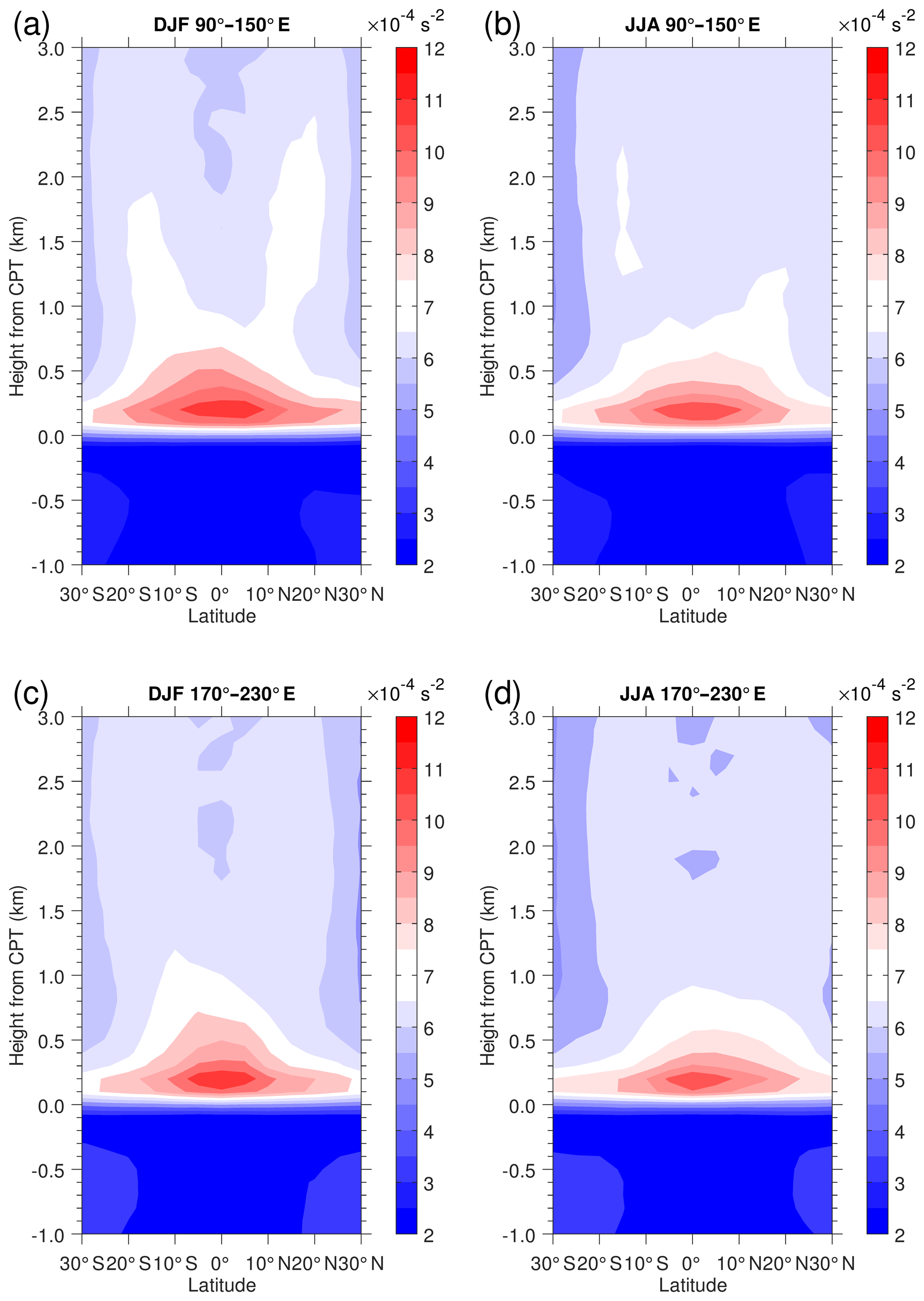
Figure 3Height–latitude cross sections of the mean N2 relative to the CPT location in the vertical for (a, c) DJF and (b, d) JJA in the two longitude regions. Color contour interval is s−2.
The profiles of large N2 near 20∘ N and 20∘ S in the MC region represent the vertical section of the Kelvin and mixed Rossby–gravity waves response known as the Matsuno–Gill pattern mode (Matsuno, 1966; Gill, 1980; Grise et al., 2010; Nishimoto and Shiotani, 2012). The results shown in Fig. 3 uncover the detailed structure of N2 above CPT in the specific longitude regions compared to the results by Grise et al. (2010) that showed the mean N2 over the 0–1 km layer above the LRT. The vertical propagation of equatorial waves (Kelvin waves and/or gravity waves), as a result of convective forcing, modulates the tropopause (Tsuda et al., 1994; Randel and Wu, 2005; Kim and Alexander, 2015; Kim et al., 2018). The MJO activity was also found to control the tropopause variability (Kim and Son, 2012; Pilch Kedzierski et al., 2016).
The N2 above the tropical tropopause in DJF is larger than in JJA in the longitude–height cross section over 10∘ S–10∘ N (not shown). The mean N2 has a maximum of about s−2 at 17.5–19.0 km, which agrees with the result by Grise et al. (2010). This height range is located around 1–2 km above the mean LRT height (16.5 km). The maxN2 of individual profiles are located mainly within 1 km above the CPT height (17.2 km). Averaging N2 in conventional height coordinates tends to smooth out the tropopause sharpness (Birner et al., 2002). Here, we describe the longitude–height cross section of N2 distribution relative to the CPT height (Fig. 4). The region of elevated N2 becomes a single thin layer with maximum value reaching s−2. Values of s−2 are more prominent in DJF than in JJA (Fig. 3). Values of s−2 at 1–2 km above CPT are shifted somewhat eastward from the maximum at 0.0–0.5 km above the CPT, especially at 120–210 and 240–300∘ E.
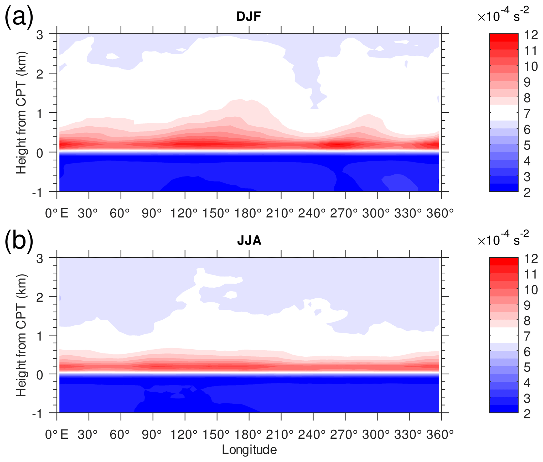
Figure 4Height–longitude cross sections of the mean N2 over 10∘ S–10∘ N latitude relative to the CPT location in the vertical for (a) DJF and (b) JJA. Color contour interval is s−2.
Figures 3 and 4 show a thin layer of low N2 within the 1 km layer below the CPT and large N2 within the 1 km layer above the CPT. In the following section we investigate the frequency distribution of TIL parameters related to the shallow layer within ±1 km of the CPT.
3.2 Frequency distribution of TIL parameters
The histograms of all TIL parameters over the period 2007–2016 for the entire longitude range at 30∘ S–30∘ N are presented in Fig. 5. All parameters show a skewed distribution. In Fig. 5 (left column), the mean S-aCPT is larger than S-bCPT. The values of S-aCPT are mostly in the range 2.8– s−2, and the values larger than its mean in the range 8.5– s−2. About 80 % of S-bCPT values lie in the range 1.7– s−2, while only about 3 % have S-bCPT s−2. The mean and standard deviation of S-ab are s−2. The tail to the right of the mean S-ab is longer than that to the left (i.e., positive skewness). The positive skewness distribution of S-ab is found to be similar to the results by Pilch Kedzierski et al. (2016) for above the LRT for both easterly and westerly QBO periods. This is reasonable since above CPT would dominate the relatively low values of below CPT, showing similar features to those of S-ab. The results indicate a large variation in the temperature gradient within 1 km above the CPT. The natural question would be when and where large values (the longer tails) appear and what atmospheric processes are responsible. In the next section, we discuss the variation in S-ab that is associated with convective activity.
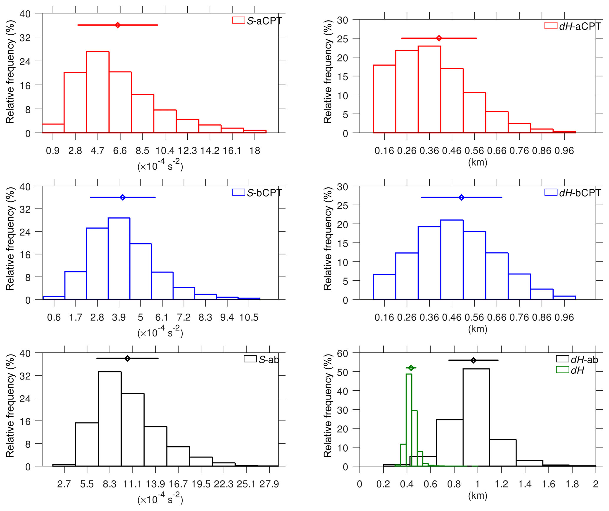
Figure 5Frequency distribution of TIL parameters with respect to the vertical distance from the CPT. The diamonds and horizontal lines above each histogram represent the mean and standard deviation of each parameter, respectively.
The distribution of dH-aCPT, which has mean and standard deviation 0.4±0.2 km, is similar to that of S-aCPT, while dH-bCPT is nearly symmetric with mean and standard deviation 0.5±0.2 km (Fig. 5, right column). About 60 % of the values of dH-aCPT lie in the range 0.2–0.4 km. That means that 60 % of maxN2 are located between the CPT and 0.4 km above it. About 70 % of the magnitudes of dH-ab are within 1.0±0.2 km. This is reasonable because dH-ab is equal to the sum of dH-aCPT and dH-bCPT, and this means the distance between the minN2 level below the CPT and the maxN2 level above CPT was 1 km. The minN2 and maxN2 are related to decreasing and increasing temperature, respectively.
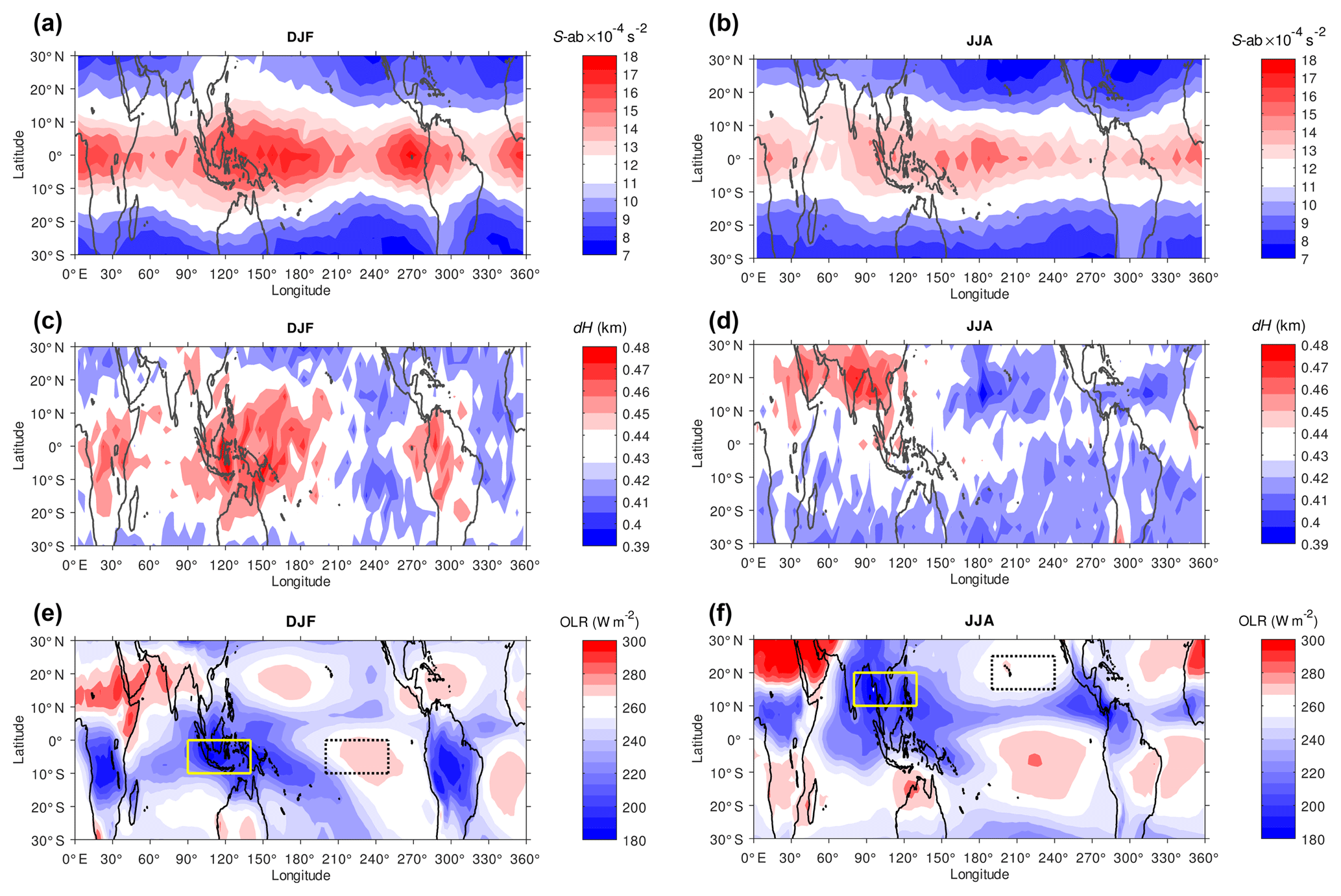
Figure 6Horizontal distribution of the mean S-ab (a, b), dH (c, d), and OLR (e, f) during Northern Hemisphere winter (DJF) and summer (JJA). Solid yellow and dotted black boxes in the bottom row indicate the sample “convective” and “nonconvective” regions, respectively.
The thickness dH varies between 0.3 and 0.6 km, but 70 % of the values are within 0.4±0.04 km (green histogram in Fig. 5, lower right panel). This result shows a very thin TIL layer above the CPT in the tropics. The thin layer of TIL can also be seen in Fig. 3. If the mean maxN2 is in the range 11– s−2 in both seasons, then 80 % of the maxN2 is about 8.8– s−2. The contour lines of N2 at this interval depict a very thin layer (<0.5 km) in both longitude regions (Fig. 3). This leads to the question of how the thickness varies in the tropics. In the following section, we investigate the climatology of S-ab and dH.
3.3 Seasonal variations in TIL sharpness and thickness
Figure 6 shows horizontal distributions of the mean S-ab, dH, and OLR in the tropics during DJF and JJA. The mean S-ab in the low latitudes during DJF is larger than that during JJA. The highest values, up to 16– s−2, are strongly associated with low OLR values, suggesting strong deep convection over the following convective regions: (i) Africa, (ii) a wide area from the Maritime Continent to the western Pacific, and (iii) South America. Large S-ab values are found along in the equatorial region, while low-OLR regions show latitudinal variation with season. Local and seasonal variability of horizontal structure of tropopause sharpness presented in this work are consistent with previous studies which attributed it to equatorial waves activity (e.g., Grise et al., 2010; Son et al., 2011; Kim and Son, 2012). However, we found different quantitative results, in particular over the western Pacific, because of the use of and instead of averaging N2 within ±1 km relative to CPT as was done in Kim and Son (2012). Maximum static stability just above the tropical tropopause could also be associated with divergence flow as demonstrated by Pilch Kedzierski et al. (2016). Large S-ab around the 240–270∘ E longitude region in DJF is qualitatively related to OLR values of 220–240 W m−2, representing the intertropical convergence zone (ITCZ). Large S-ab values of 14– s−2 are also found over South Asia and near the ITCZ in JJA. Exception is seen over South America where S-ab only reaches s−2 associated with OLR values <220 W m−2. Radiative effects from cirrus cloud may be responsible for the enhancement of S-ab. Sassen et al. (2009) demonstrated that cirrus clouds are confined to the monsoon region and ITCZ where they are generated in anvils created by deep convection. The cirrus cloud decreases the static stability below the tropopause (Nishimoto and Yoden, 2017; Son et al., 2017). Therefore, decreasing static stability below the tropopause will tend to enlarge the difference between and .
Bell and Geller (2008) investigated the thickness defined as the distance from the LRT to the level where dN2∕dz reached its minimum in the stratosphere (z is the vertical coordinate) using global interpolated radiosonde data. They reported a thickness of ∼1 km at latitudes around 15∘ N. Since there are few radiosonde stations in the low latitudes, they did not show the horizontal distribution of the thickness. Here, we use a different definition of dH as explained in Sect. 2. In Fig. 6 (middle row), values of dH lie in the range 0.39–0.48 km. Large dH associated with low OLR values over the three convective regions agrees qualitatively with large S-ab.
Deep convection over Indonesia and northern Australia near Darwin during the Australian monsoon (DJF) and over the Bay of Bengal, South Asia, and the Philippines during the Asian monsoon (JJA) seems to be the main control on S-ab and dH. To emphasize the effect of convective activity, we show the mean N2 profiles in DJF and JJA in Fig. 7. We define 90–140∘ E, 10∘ S–0 in DJF and 80–130∘ E, 10–20∘ N in JJA as the “convective” regions (OLR ≤240 W m−2). The “nonconvective” regions (OLR >240 W m−2) are 200–250∘ E, 10∘ S–0 in DJF and 190–240∘ E, 15–25∘ N in JJA. We selected those regions as described in Fig. 6 (bottom row), each with the same area (50∘ longitude latitude). The total numbers of profiles from 10 years of COSMIC GPS-RO observation inside the convective regions are 9140 in DJF and 18 046 in JJA, while inside the nonconvective regions there are 8758 profiles in DJF and 17 103 in JJA. COSMIC satellites operate in polar orbits, so the highest numbers of profiles are located in the midlatitudes (e.g., Fig. 1 in Son et al., 2011). The total numbers of profiles in JJA are larger than in DJF because the convective and nonconvective regions in JJA are defined to lie closer to the midlatitudes. It is clear that in both DJF and JJA the mean N2 over the convective regions is smaller below the CPT and larger above CPT than the mean N2 over the nonconvective regions. The difference in the mean N2 is s−2 below the CPT and s−2 near the level of maxN2 above the CPT. The observations show that regions with more frequent convective activity show decreased N2 below CPT and increased , which increased S-ab from to s−2 and tended to increase dH from 0.3 to 0.5 km.
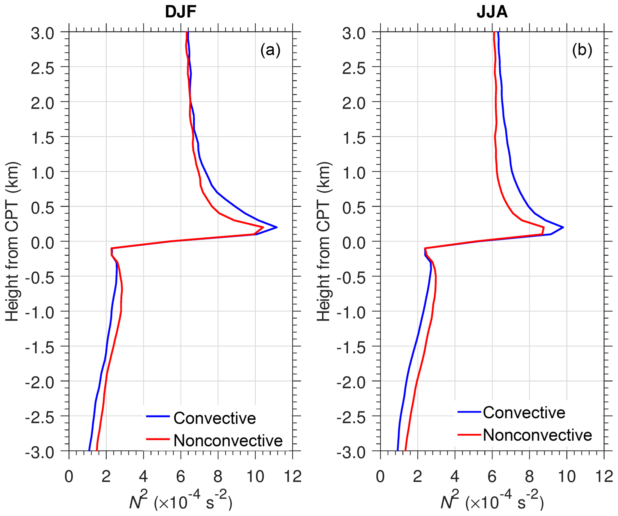
Figure 7Mean N2 profiles over the convective and nonconvective regions defined in Fig. 10 for DJF (a) and JJA (b).
We have examined the spatial distributions of S-ab and dH in boreal winter and summer. To show the seasonal cycle in the different longitude regions, we calculated the monthly mean and standard deviation of S-ab and dH over 10∘ S–10∘ N as shown in Fig. 8. We repeat two seasonal cycles in Fig. 8 to display seasonal cycle more clearly. The sharpness and thickness are greater in MC than in PO. The sharpness in MC during July–August is somewhat higher than in May–June and September–October, while it is relatively constant at s−2 in PO from March to November. It is also clear that the seasonal cycle in the MC is affected by the subseasonal variation. On the other hand, the thickness in PO shows a clear annual cycle with a minimum in JJA. The results indicate that land–sea distribution influences the variability in S-ab and dH.
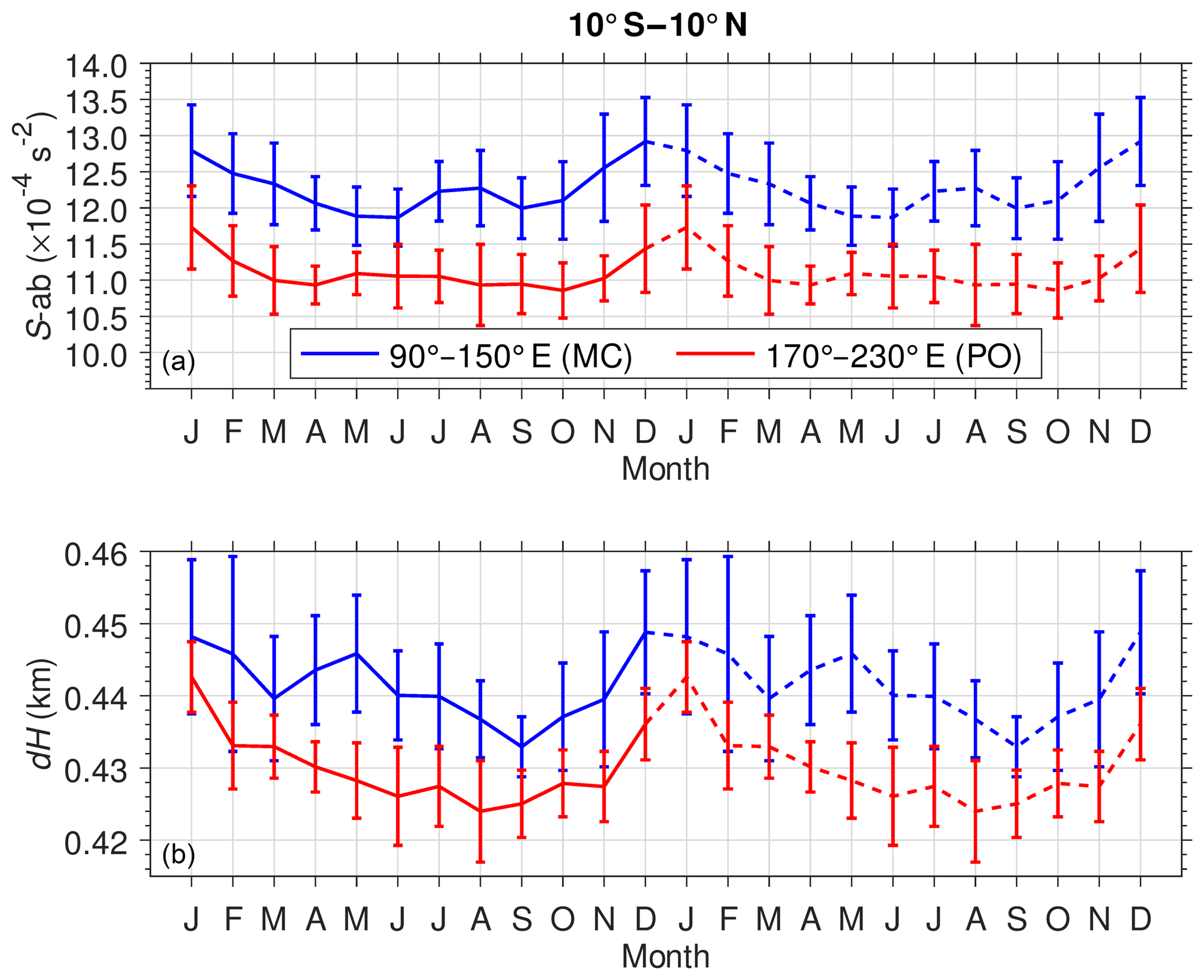
Figure 8Seasonal variation in the mean S-ab (a) and dH (b) over the MC (blue line) and the PO (red line). Error bars show the standard deviation with respect to the mean value. Note that both S-ab and dH are duplicated to show the seasonal cycle more clearly (dashed line).
In the following section we discuss the interannual and intraseasonal variability of S-ab.
3.4 Influence of El Niño and La Niña
We investigate the monthly mean S-ab as well as OLR data in the two longitude regions (Fig. 9). Large S-ab in the MC associated with low OLR values can be seen during NH winter as part of the annual cycle. Neither the annual peak of S-ab nor the peak of low OLR over the MC is seen in DJF for 2009–2010. On the other hand, S-ab increased from to s−2 over the PO in the same period. This suggests a signal of interannual variation in S-ab and OLR in both the MC and PO. Another signal that can be interpreted as interannual variation is seen in DJF of 2015–2016, where S-ab showed a strong peak and convective activity was also enhanced in the PO. The linear correlation between S-ab and OLR in the MC and PO has coefficients of −0.57 and −0.67, respectively, delineating an out-of-phase relation. We have tested for different lags. The cross-correlation between S-ab and OLR becomes smaller when a 2-month lag occurs (−0.49 and −0.57 over MC and PO regions, respectively).

Figure 9Time series of monthly mean S-ab (solid blue line) and OLR (dotted red line) for the MC (a) and PO (b).
The negative correlation from the monthly mean time series may still be affected by the annual cycle or intraseasonal variation. Therefore, we investigate the S-ab and OLR anomalies (S-ab∗ and OLR∗) calculated by subtracting the climatological values from the monthly mean time series. Next, we compare both S-ab∗ and OLR∗ with the SST Niño 3.4 index (Fig. 10). We applied a 4-month running mean to smooth the time series and reduce the possible intraseasonal fluctuation, as subtracting the climatological mean will only remove the annual cycle. El Niño events were defined when SST Niño 3.4 . Strong El Niño events occurred during the NH winters 2009–2010 and 2015–2016. La Niña events were determined when SST Niño 3.4 . La Niña events were seen during the NH winters 2007–2008, 2008–2009, and 2010–2011. A linear correlation analysis shows that S-ab∗ is negatively correlated with both OLR∗ (−0.56) and SST Niño 3.4 (−0.66) in the MC. Surprisingly, in the PO, S-ab∗ is strongly negatively correlated with OLR∗ (−0.90) and strongly positively correlated with SST Niño 3.4 (+0.88). The negative and positive correlations between S-ab∗ and SST Niño 3.4 show that El Niño and La Niña phenomena have a significant impact on the variation in S-ab∗. The high magnitude of the correlation for PO could be due to the fact that, outside ENSO events, this is a region with very low convective activity, whereas MC is not devoid of convection even during ENSO events (and MJO can influence the MC region as well in its late phases). The negative correlation between S-ab∗ and OLR∗, which is modulated by SST Niño 3.4, means that convective activity on the interannual timescale influences S-ab∗ in both longitude regions.
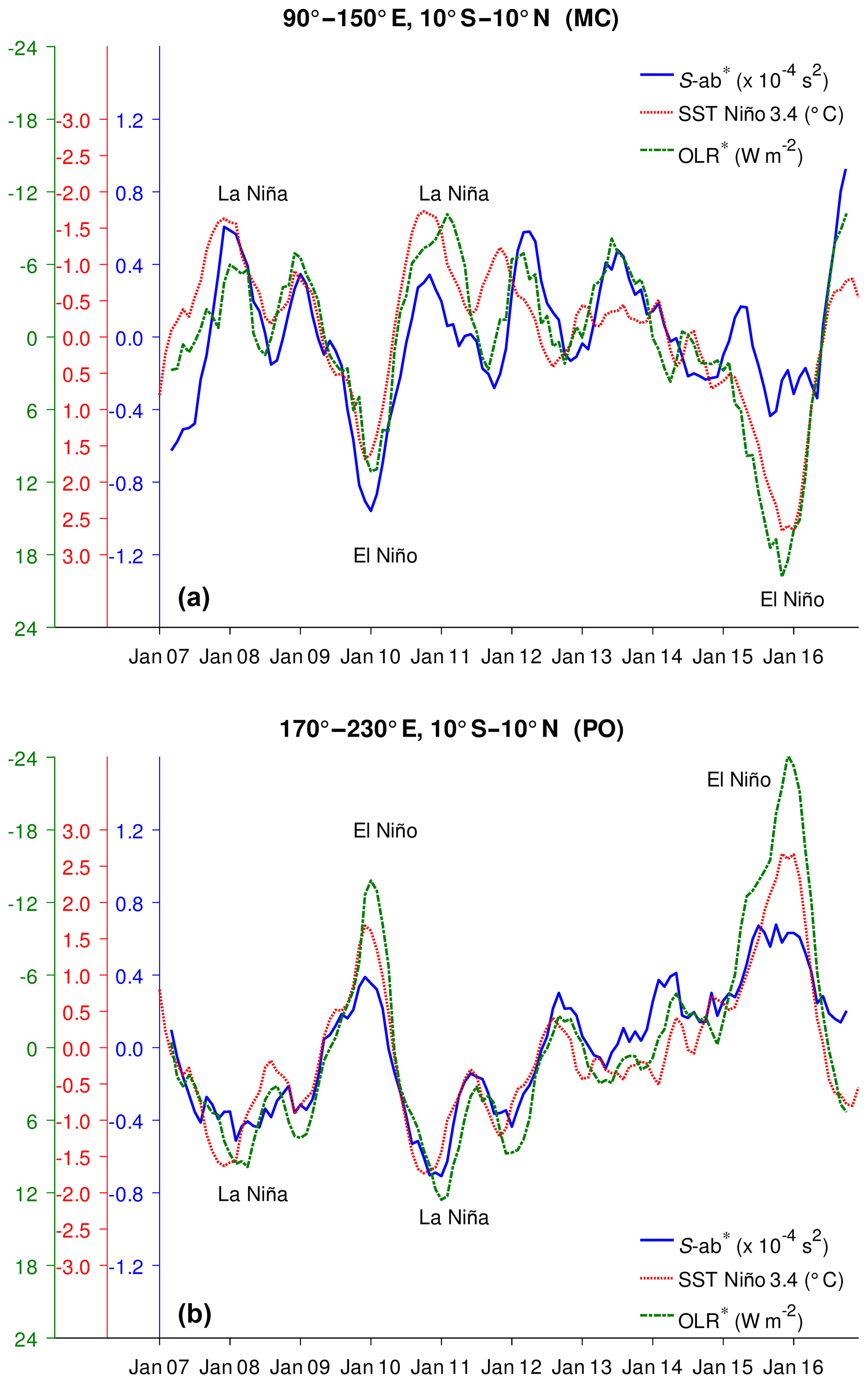
Figure 10Interannual variations in a S-ab anomaly (S-ab∗) (solid blue line), OLR anomaly (OLR∗) (dashed-dotted green line), and SST Niño 3.4 index (dotted red line) for the MC (a) and PO (b). Note that the ordinate axes of both OLR∗ and SST Niño 3.4 index are reversed in panel (a), but only the ordinate axis of OLR∗ is reversed in panel (b).
To analyze in more detail the influence of El Niño and La Niña, we calculate the mean N2 profile over the MC and PO during DJF El Niño and DJF La Niña (Fig. 11). The mean N2 during La Niña events below the CPT was smaller and above the CPT was larger than during El Niño events over the MC, as more convection occurred. Under La Niña conditions, the mean maxN2 overshoots up to s−2 and relaxes gradually to the lowermost stratospheric value of s−2 at 2 km above the CPT. However, under El Niño conditions the mean maxN2 is s−2 and sharply decreases to s−2 about 0.5 km above the CPT. Convective clouds that are more active during El Niño in the PO than during La Niña are the cause of the difference in mean N2 profiles between these two cases shown in Fig. 11b. The maxN2 in El Niño was s−2, larger than in La Niña ( s−2), but in both cases the values of N2 sharply decrease and then coincide at the lowermost stratospheric value at ∼1 km above the CPT. The results show that convective activity in both longitude regions during El Niño and La Niña will extend the above the CPT so that S-ab increases from to s−2.
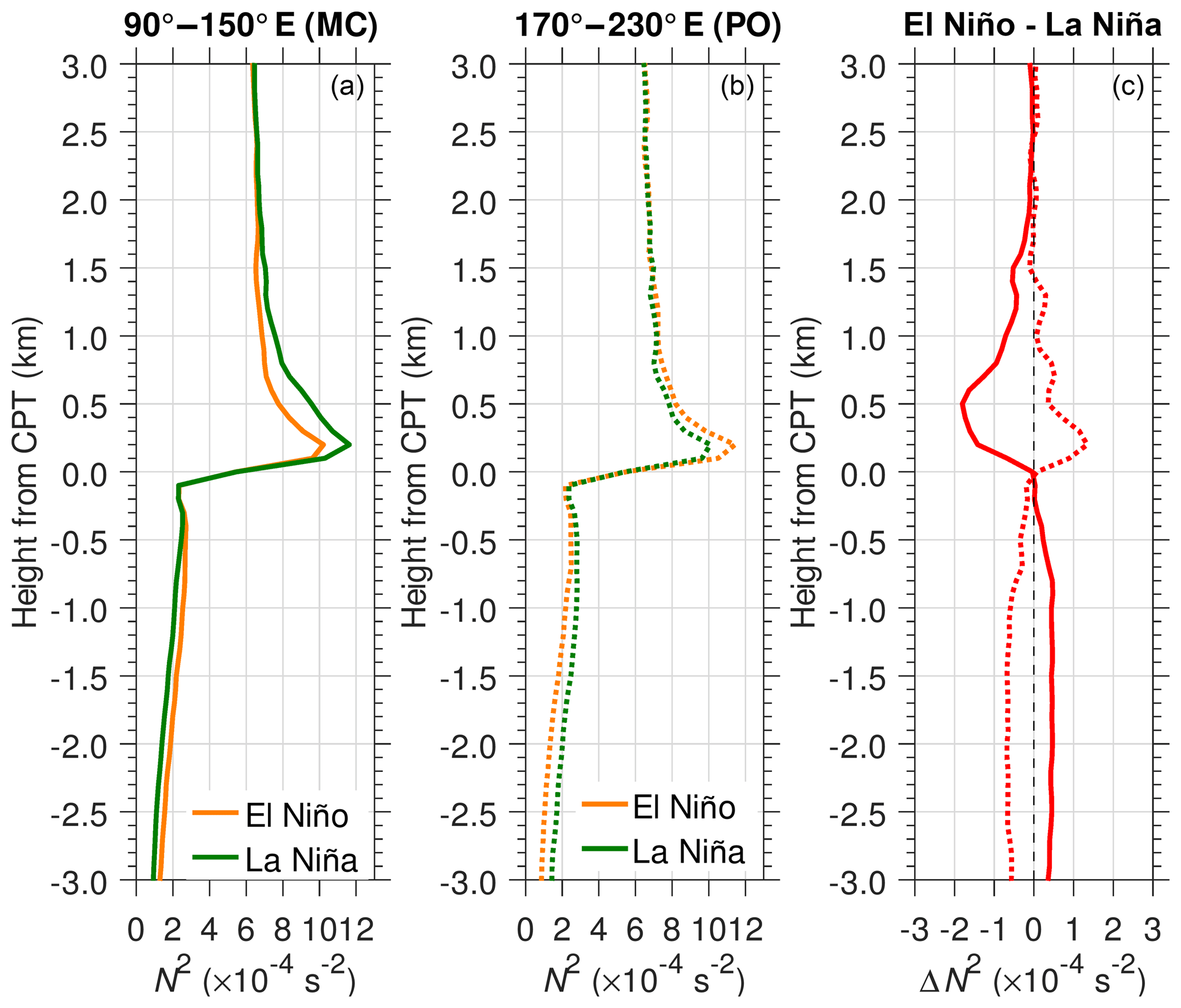
Figure 11Mean N2 profiles during DJF El Niño (a) and DJF La Niña (b). Difference between the mean N2 in DJF El Niño and in DJF La Niña (c) in the MC (solid line) and PO (dotted line).
Figure 11c shows the difference in the mean N2 (ΔN2) between El Niño and La Niña events. In the MC and PO, the ΔN2 below the CPT is s−2 in both cases. We found that above the CPT the peak amplitude ΔN2 in the MC regions is higher and larger (0.5 km above the CPT and s−2) than in the PO region (0.2 km above CPT and s−2). The difference in the thermal structure near tropopause over land and ocean may cause the difference in peak amplitude of ΔN2 above the CPT. One possibility is that the mountainous characteristics of the MC region are favorable to generate convectively coupled equatorial waves (Kubokawa et al., 2016). Other possible processes are as follows. Warmer SST under La Niña conditions results in more active convection that tends to force air upward to the TTL and then decrease the static stability below the CPT. The stratospheric air resists a change in height, so the temperature gradient becomes greater, enhancing maxN2 above the CPT. Although our analysis is based on limited observations, the results indicate that tropopause sharpness is correlated with convective activity associated with El Niño and La Niña phenomena.
3.5 MJO modulation
The convective activity in the tropics is also influenced by intraseasonal variability (Wheeler and Kiladis, 1999). We extend our analysis to the intraseasonal variation in tropopause sharpness related to MJO propagation in the tropics. An MJO active phase is represented by large-scale deep convection that moves eastward, while an inactive phase is marked by suppressed convection (Zhang, 2005). Organized convective clouds propagate from the Indian Ocean to the western Pacific from phase 3 to phase 6, as defined by Wheeler and Hendon (2004), over a period of ≤10 d or within 10–15 d during fast MJO episodes. During slow MJO episodes the propagation takes more than 20 d (Yadav and Straus, 2017). To identify fast or slow MJO events, we use OMI data because they are derived directly from OLR and represent the convective signal of MJO (Kiladis et al., 2014). Figure 12 shows a case study for a slow MJO episode from 1 December 2007 to 28 February 2008 and a fast MJO episode from 15 January 2012 to 15 April 2012. The figure shows the propagation for both MJO active and inactive phases. In this figure, we obtained S-ab∗ by subtracting the average of S-ab over 120 d from the 5 d running mean time series. We applied a band-pass filter to the fluctuation components of S-ab with a cut-off frequency of 30–90 d to retain MJO phase propagation (Kiladis et al., 2014; Zhang, 2005). The same analysis was applied to the OLR data.

Figure 12Time–longitude distribution (Hovmöller diagram) of S-ab∗ (color shading) and OLR∗ (dotted contours). Color contour interval is s−2 and only negative values of OLR∗ are shown for −35, −25, −15, −5, and −2.5 W m−2.
Enhancement of S-ab∗ is obviously associated with eastward propagation of organized deep convection from the western Indian Ocean to the central Pacific during December 2007 and January 2008 (∼60 d), which is classified as a slow MJO episode (Fig. 12a). During the fast MJO episode (Fig. 12b), eastward movement of large positive S-ab∗ also coincided with negative OLR∗ from 23 January to 8 February 2012 (a period of 17 d). When the deep convection was suppressed during the inactive phase, S-ab∗ decreased. Zeng et al. (2012) demonstrated a low-temperature anomaly observed with COSMIC near the tropopause associated with a rainfall anomaly during MJO active-phase propagation. Kim and Son (2012) and Pilch Kedzierski et al. (2016) also found that the MJO signal modulates the tropopause temperature and sharpness structure using COSMIC temperature data. We found that the MJO propagation in the tropics has an impact on the variability in tropopause sharpness, being consistent with the results by Pilch Kedzierski et al. (2016). Note that we demonstrated the time evolution of the positive sharpness anomaly associated with negative OLR anomaly, which is not shown in the previous studies (Kim and Son, 2012; Pilch Kedzierski et al., 2016). A strong correlation between S-ab∗ and OLR∗ propagation on the intraseasonal timescale indicates that the organized deep convection reaches the upper troposphere and tends to enhance the temperature gradient in the TTL.
We investigated the N2 profiles over the MC during the MJO active (5–15 January 2008) and MJO inactive (15–25 February 2008) phases. Figure 13 shows the characteristics of the difference in the mean N2 between the periods of strong and weakened convection over the MC. The difference in the mean N2 (ΔN2) between the MJO active and inactive phases shows negative values of s−2 at 1–3 km below the CPT, then jumps to s−2 within 0.5 km above the CPT, suggesting that convection tends to lower the static stability below the CPT and increase the static stability just above it. It is well known that the vertical structure of temperature perturbations associated with deep convection indicates a warm anomaly in the middle and upper troposphere and cold anomaly near the tropopause (e.g., Holloway and Neelin, 2007; Paulik and Birner, 2012). Adiabatic cooling near the tropopause is a natural response of the diabatic warming due to convection as a result of hydrostatic adjustment (Holloway and Neelin, 2007). Kim et al. (2018) hypothesized that a cold anomaly near the tropopause associated with organized deep convection during the MJO active phase is due to dehydration processes. This explains the large values of S-ab of s−2 that form part of the long tail in the frequency distribution (Fig. 5).
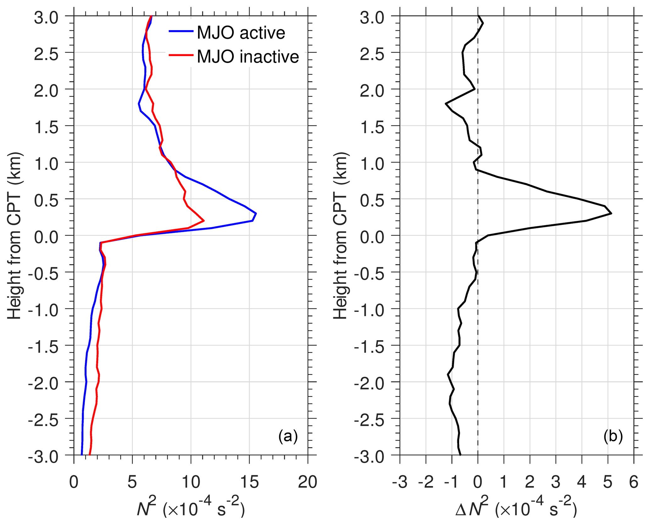
Figure 13Mean N2 profiles during MJO active (blue) and MJO inactive (red) phases (a) and their difference (b).
To show the relationship between the convective activity and tropopause sharpness in MC and PO regions at intraseasonal (Fig. 12) through to interannual timescales (Fig. 10), we provide the diagrams in Fig. 14 which are analogous to Fig. 3 of Pilch Kedzierski et al. (2016), which showed sharpness versus divergence near the tropopause, and to Fig. 5 of Randel et al. (2007), which demonstrated sharpness versus vorticity in the extratropics. Figure 14 displays the scatter plot of S-ab versus OLR in all seasons. As expected, large S-ab values at range 9– s−2 associated with OLR values of 250–150 W m−2 for the number of sample >180. We have also investigated the slope of relationship between S-ab and OLR in Fig. 14a and b for the number of samples ≥500. Both slopes show only slightly difference between MC and PO regions, indicating that the variability of deep convection is the major cause of tropopause sharpness variability.
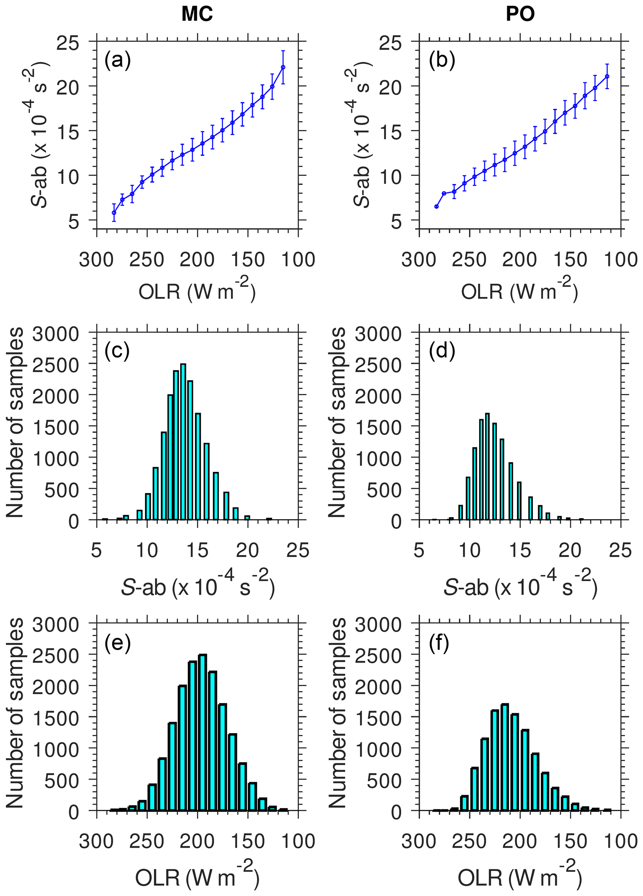
Figure 14Diagram of S-ab versus OLR (a, b), and of the number of samples for S-ab and OLR (c, d and e, f, respectively) in the MC (a, c, e) and PO (b, d, f) regions.
COSMIC GPS-RO data retrieved using full spectrum inversion (cosmicfsi) provide 0.1 km vertical resolution temperature profiles (T) in the UTLS. Using these data for 2007 to 2016, we investigated the distribution of N2 in the TTL and the variation in the tropical TIL. We showed that cosmicfsi captured small-scale fluctuations in the individual N2 as seen in radiosonde observations (Fig. 1). We demonstrated the characteristics of N2 over the MC and PO relative to the CPT height. The maximum of the mean N2 changed is s−2 within 1 km above the CPT. Latitudinal and longitudinal distributions show that N2 above the CPT in DJF was larger than in JJA (Figs. 3 and 4). The results generally agree very well with previous studies (Grise et al., 2010; Birner, 2006; Birner et al., 2002). Using datasets with improved vertical resolution, we found larger values of N2 compared to the results by Grise et al. (2010) in this study.
We found that ∼60 % of maxN2 values were located within 0.5 km above the CPT. The frequency distribution of the tropopause sharpness (S-ab) has a positive skewness with a longer tail to the right of the mean than to the left. The mean and standard deviation of S-ab are s−2 (Fig. 5). This suggests a large variation in the temperature gradient within ±1 km of the CPT. Typical TIL thickness (dH) values are in the range within 0.5 km. Analysis of the seasonal variation shows that large S-ab and large dH are associated with deep convection during the Australian and Asian monsoons (Fig. 6). In convective regions the mean N2 is smaller below the CPT and larger above the CPT than in nonconvective regions.
We analyzed the interannual variation in S-ab (S-ab∗) and OLR (OLR∗) anomalies, and the SST Niño 3.4 index. We found an out-of-phase relation between S-ab∗ and OLR∗ over both the Maritime Continent (MC) and Pacific Ocean (PO), with correlation coefficients of −0.56 and −0.90, respectively. S-ab∗ in the MC was negatively correlated with SST Niño 3.4 (−0.66), while in the PO it was in-phase and strongly correlated (+0.88) (Fig. 10). We also calculated the mean N2 over the MC and PO during DJF El Niño and DJF La Niña. The results indicate that during La Niña over the MC and El Niño over the PO, warmer SST gives more convection that tends to drive air upward into the TTL and increases the temperature gradient (positive S-ab∗).
We also analyzed the intraseasonal variation in S-ab∗. Case studies during slow and fast MJO episodes show strong eastward propagation of S-ab∗ associated with deep convection. Meanwhile, when organized deep convection is suppressed in the MJO inactive phase, S-ab∗ decreases (Fig. 12). This suggests that the variations in S-ab∗ in the tropics are strongly related to the convective activity at this timescale. We showed the influence of ENSO and MJO on the variation in TIL that has not been studied previously. The diagram of S-ab versus OLR both in the MC and PO regions during all seasons indicates that the variability of convective activity in the tropics is a major influence on tropopause structure at various timescales (Fig. 14).
The cosmic2013 are open in the CDAAC UCAR website (https://cdaac-www.cosmic.ucar.edu/cdaac/products.html, last access: 17 May 2019). The cosmicfsi data provided by RISH Kyoto University (http://database.rish.kyoto-u.ac.jp/arch/iugonet/GPS/index.html, last access: 8 July 2017) that has been registered in IUGONET database system (http://search.iugonet.org/list.jsp, last access: 8 July 2017). All radiosonde data were downloaded from the Earth Observing Laboratory (http://data.eol.ucar.edu/dataset/347.123, last access: 26 February 2016). SST Nino 3.4 index is obtained from http://www.cpc.ncep.noaa.gov/data/indices/ (last access: 9 August 2018). OLR MJO Index are available at https://www.esrl.noaa.gov/psd/mjo/mjoindex/ (last access: 1 November 2017).
N performed the analysis, created the figures and wrote the manuscript. TT and MF contributed to the text and provided guidance. All authors read and approved the final paper.
The authors declare that they have no conflict of interest.
Fruitful discussion with Shigeo Yoden is acknowledged. Noersomadi received a scholarship from the Research and Innovation in Science and Technology Project (Riset-Pro) from the Ministry of Research, Technology and Higher Education (Kemenristekdikti) of Indonesia.
This research has been supported by the Japan Society for the Promotion of Science (grant no. JP18K03741).
This paper was edited by Peter Haynes and reviewed by three anonymous referees.
Andrews, D. G., Holton, J. R., and Leovy, C. B.: Middle atmosphere dynamics, International Geophysics Series, vol. 40, Academic Press, Cambridge, UK, 1987.
Anthes, R. A.: Exploring Earth's atmosphere with radio occultation: contributions to weather, climate and space weather, Atmos. Meas. Tech., 4, 1077–1103, https://doi.org/10.5194/amt-4-1077-2011, 2011.
Bernhardt, P. A., Chen, Y., Cucurull, L., Dymond, K. F., Ector, D., Healy, S. B., Ho, S.-P., Hunt, D. C., Kuo, Y.-H., Liu, H., Manning, K., McCormick, C., Meehan, T. K., Randel, W. J., Rocken, C., Schreiner, W. S., Sokolovskiy, S. V., Syndergard, S., Thompson, D. C., Trenberth, K. E., Wee, T.-K., Yen, N. L., and Zeng, Z.: The COSMIC/FORMOSAT-3 mission: Early results, B. Am. Meteorol. Soc., 89, 313–333, https://doi.org/10.1175/BAMS-89-3-313, 2008.
Bell, S. W. and Geller, M. A.: Tropopause inversion layer: Seasonal and latitudinal variations and representation in standard radiosonde data and global models, J. Geophys. Res.-Atmos., 113, 1–7, https://doi.org/10.1029/2007JD009022, 2008.
Birner, T.: Fine-scale structure of the extratropical tropopause region, J. Geophys. Res., 111, D04104, https://doi.org/10.1029/2005JD006301, 2006.
Birner, T., Dörnbrack, A., and Schumann, U.: How sharp is the tropopause at midlatitudes?, Geophys. Res. Lett., 29, 1700, https://doi.org/10.1029/2002GL015142, 2002.
Butchart, N.: The Brewer-Dobson circulation, Rev. Geophys, 52, 157–184, https://doi.org/10.1002/2013RG000448, 2014.
Fritts, D. C., Tsuda, T., Sato, T., Fukao, S., and Kato, S.: Obervational evidence of a saturated gravity wave spectrum in the troposphere and lower stratosphere, J. Atmos. Sci., 45, 1741–1759, 1988.
Fueglistaler, S., Dessler, A. E., Dunkerton, T. J., Folkins, I., Fu, Q., and Mote, P. W.: Tropical tropopause layer, Rev. Geophys. 47, RG1004, https://doi.org/10.1029/2008RG000267, 2009.
Fujiwara, M. and Takahashi, M.: Role of the equatorial Kelvin wave in stratosphere-troposphere exchange in a general circulation model, J. Geophys. Res.-Atmos., 106, 22763–22780, https://doi.org/10.1029/2000JD000161, 2001.
Gettelman, A. and Wang, T.: Structural diagnostics of the tropopause inversion layer and its evolution, J. Geophys. Res., 120, 46–62, https://doi.org/10.1002/2014JD021846, 2015.
Gill, A. E.: Some simple solutions for heat-induced tropical circulation, Q. J. Roy. Meteor. Soc., 106, 447–462, 1980.
Gong, J. and Geller, M. A.: Vertical fluctuation energy in United States high vertical resolution radiosonde data as an indicator of convective gravity wave sources, J. Geophys. Res., 115, D11110, https://doi.org/10.1029/2009JD012265, 2010.
Gorbunov, M. E.: Radio-holographic analysis of Microlab-1 radio occultation data in the lower troposphere, J. Geophys. Res., 107, 4156, https://doi.org/10.1029/2001JD000889, 2002.
Grise, K. M., Thompson, D. W. J., and Birner, T.: A global survey of static stability in the stratosphere and upper troposphere, J. Climate, 23, 2275–2292, https://doi.org/10.1175/2009JCLI3369.1, 2010.
Hayashi, H., Koyama, Y., Hori, T., Tanaka, Y., Abe, S., Shinbori, A., Kagitani, M., Kouno, T., Yoshida, D., Ueno, S., Kaneda, N., Yoneda, M., Umemura, M., Tadokoro, H., and Motoba, T.: Inter-University upper Atmosphere Global Observation Network (IUGONET), Data Science Journal, 12, WDS179–WDS184, https://doi.org/10.2481/dsj.WDS-030, 2013.
Holloway, C. E. and Neelin, J. D.: The convective cold top and quasi equilibrium, J. Atmos. Sci., 64, 1467–1487, https://doi.org/10.1175/JAS3907.1, 2007.
Holton, J. R., Haynes, P. H., Mcintyre, M. E., Douglass, A. R., Rood, R. B., and Pfister, L.: Stratosphere-Troposphere Exchange, Rev. Geophys., 403–439, 1995.
Jensen, A. S., Lohmann, M. S., Benzon, H. H., and Nielsen, A. S.: Full spectrum inversion of radio occultation signals, Radio Sci., 38, 1–15, https://doi.org/10.1029/2002RS002763, 2003.
Jensen, A. S., Lohmann, M. S., Nielsen, A. S., and Benzon, H. H.: Geometrical optics phase matching of radio occultation signals, Radio Sci., 39, 1–8, https://doi.org/10.1029/2003RS002899, 2004.
Kiladis, G. N., Dias, J., Straub, K. H., Wheeler, M. C., Tulich, S. N., Kikuchi, K., Weickmann, K. M., and Ventrice, M. J.: A Comparison of OLR and Circulation-Based Indices for Tracking the MJO, Mon. Weather Rev., 142, 1697–1715, https://doi.org/10.1175/MWR-D-13-00301.1, 2014.
Kim, J. and Son, S.-W.: Tropical cold-point tropopause: Climatology, seasonal cycle, and intraseasonal variability derived from COSMIC GPS radio occultation measurements, J. Climate, 25, 5343–5360, https://doi.org/10.1175/JCLI-D-11-00554.1, 2012.
Kim, J., Randel, W. J., and Birner, T.: Convectively driven tropopause-level cooling and its influences on stratospheric moisture, J. Geophys. Res.-Atmos., 123, 590–606, https://doi.org/10.1002/2017JD027080, 2018.
Kim, J.-E. and Alexander, M. J.: Direct impacts of waves on tropical cold point tropopause temperature, Geophys. Res. Lett., 42, 1584–1592, https://doi.org/10.1002/2014GL062737, 2015.
Kubokawa, H., Satoh, M., Suzuki, J., and Fujiwara, M.: Influence of topography on temperature variations in the tropical tropopause layer, J. Geophys. Res.-Atmos., 121, 11556–11574, https://doi.org/10.1002/2016JD025569, 2016.
Kursinski, E. R., Hajj, G. A., Schofield, J. T., Linfield, R. P., and Hardy, K. R.: Observing Earth's atmosphere with radio occultation measurements using the Global Positioning System, J. Geophys. Res., 102, 23429-23465, https://doi.org/10.1029/97JD01569, 1997.
Liebmann, B. and Smith, C. A.: Description of a complete (interpolated) outgoing longwave radiation dataset, B. Am. Meteorol. Soc., 77, 1275–1277, 1996.
Matsuno, T.: Quasi-geostrophic motions in the equatorial area, J. Meteorol. Soc. Jpn., 44, 25–42, 1966.
Melbourne, W. G.: Radio occultation using earth satellites, Wiley, New Jersey, USA, 2004.
Mote, P. W., Rosenlof, K. H., Mclntyre, M. E., Carr, E. S., Gille, J. C., Holton, J. R., Kinnersley, S., Pumphrey, H. C., Russel III, J. M., and Waters, J. W.: The imprint of tropical tropopause temperatures on stratospheric water vapor, J. Geophys. Res, 101, 3989–4006, 1996.
Nishimoto, E. and Shiotani, M.: Seasonal and interannual variability in the temperature structure around the tropical tropopause and its relationship with convective activities, J. Geophys. Res., 117, 1–11, https://doi.org/10.1029/2011JD016936, 2012.
Nishimoto, E. and Yoden, S.: Influence of the stratospheric quasi-biennial oscillation on the Madden–Julian oscillation during Austral summer, J. Atmos. Sci., 74, 1105–1125, https://doi.org/10.1175/JAS-D-16-0205.1, 2017.
Noersomadi and Tsuda, T.: Comparison of three retrievals of COSMIC GPS radio occultation results in the tropical upper troposphere and lower stratosphere, Earth Planets Space, 69, 1–15, https://doi.org/10.1186/s40623-017-0710-7, 2017.
Paulik, L. C. and Birner, T.: Quantifying the deep convective temperature signal within the tropical tropopause layer (TTL), Atmos. Chem. Phys., 12, 12183–12195, https://doi.org/10.5194/acp-12-12183-2012, 2012.
Pilch Kedzierski, R., Matthes, K., and Bumke, K.: The tropical tropopause inversion layer: variability and modulation by equatorial waves, Atmos. Chem. Phys., 16, 11617–11633, https://doi.org/10.5194/acp-16-11617-2016, 2016.
Randel, W. J. and Wu, F.: Kelvin wave variability near the equatorial tropopause observed in GPS radio occultation measurements, J. Geophys. Res., 110, D03102, https://doi.org/10.1029/2004JD005006, 2005.
Randel, W. J., Wu, F., and Rios, W. R.: Thermal variability of the tropical tropopause region derived from GPS/MET observations, J. Geophys. Res., 108, 4024, https://doi.org/10.1029/2002JD002595, 2003.
Randel, W. J., Wu, F., and Forster, P.: The extratropical tropopause inversion layer: Global observations with GPS Data, and a radiative forcing mechanism, J. Atmos. Sci., 64, 4489–4496, https://doi.org/10.1175/2007JAS2412.1, 2007.
Ratnam, M. V., Tsuda, T., Shiotani, M., and Fujiwara, M.: New characteristics of the tropical tropopause revealed by CHAMP/GPS Measurements, SOLA, 1, 185–188, https://doi.org/10.2151/sola.2005-048, 2005.
Sassen, K., Wang, Z., and Liu, D.: Global distribution of cirrus clouds from CloudSat/cloud-aerosol lidar and infrared pathfinder satellite observations (CALIPSO) measurements, J. Geophys. Res.-Atmos., 114, 1–12, https://doi.org/10.1029/2008JD009972, 2009.
Scherllin-Pirscher, B., Deser, C., Ho, S. -P., Chou, C., Randel, W., and Kuo, Y. -H.: The vertical and spatial structure of ENSO in the upper troposphere and lower stratosphere from GPS radio occultation measurements, Geophys. Res. Lett., 39, 2–7, https://doi.org/10.1029/2012GL053071, 2012.
Schmidt, T., Heise, S., Wickert, J., Beyerle, G., and Reigber, C.: GPS radio occultation with CHAMP and SAC-C: global monitoring of thermal tropopause parameters, Atmos. Chem. Phys., 5, 1473–1488, https://doi.org/10.5194/acp-5-1473-2005, 2005.
Shiotani, M. and Horinouchi, T.: Kelvin wave activity and the quasi-biennial oscillation in the equatorial lower stratosphere, J. Meteorol. Soc. Jpn., 75, 175–182, 1993.
Smith, S. A., Fritts, D. C., and VandZandt, T. E.: Evidence for a saturated spectrum of atmospheric gravity waves, J. Atmos. Sci., 44, 1404–1410, 1987.
Sokolovskiy, S., Schreiner, W., Zeng, Z., Hunt, D., Kuo, Y.-H., Meehan, T. K., Stecheson, T. W., Manucci, A. J., and Ao, C. O.: Use of the L2C signal for inversions of GPS radio occultation data in the neutral atmosphere, GPS Solut., 18, 404–416, https://doi.org/10.1007/s10291-013-0340-x, 2014.
Son, S.-W., Tandon, N. F., and Polvani, L. M.: The fine-scale structure of the global tropopause derived from COSMIC GPS radio occultation measurements, J. Geophys. Res.-Atmos., 116, 1–17, https://doi.org/10.1029/2011JD016030, 2011.
Son, S.-W., Lim, Y., Yoo, C., Hendon, H. H., and Kim, J.: Stratospheric control of the madden-julian oscillation, J. Climate, 30, 1909–1922, https://doi.org/10.1175/JCLI-D-16-0620.1, 2017.
Trenberth, K. E.: The Definition of El Niño, B. Am. Meteorol. Soc., 78, 2771–2777, 1997.
Tsuda, T., Murayama, Y., Wiryosumarto, H., Harijono, S. W. B., and Kato, S.: Radiosonde observations of equatorial atmosphere dynamics over Indonesia: 1. Equatorial waves and diurnal tides, J. Geophys. Res., 99, 10491–10505, https://doi.org/10.1029/94JD00355, 1994.
Tsuda, T., Lin, X., Hayashi, H., and Noersomadi: Analysis of vertical wave number spectrum of atmospheric gravity waves in the stratosphere using COSMIC GPS radio occultation data, Atmos. Meas. Tech., 4, 1627–1636, https://doi.org/10.5194/amt-4-1627-2011, 2011.
Venkat Ratnam, M., Tsuda, T., Kozu, T., and Mori, S.: Long-term behavior of the Kelvin waves revealed by CHAMP/GPS RO measurements and their effects on the tropopause structure, Ann. Geophys., 24, 1355–1366, https://doi.org/10.5194/angeo-24-1355-2006, 2006.
Wang, W., Matthes, K., Schmidt, T., and Neef, L.: Recent variability of the tropical tropopause inversion layer, Geophys. Res. Lett., 40, 6308–6313, https://doi.org/10.1002/2013GL058350, 2013.
Wheeler, M. and Kiladis, G. N.: Convectively coupled equatorial waves: Analysis of clouds and temperature in the wavenumber–frequency domain, J. Atmos. Sci., 56, 374–399, 1999.
Wheeler, M. C. and Hendon, H. H.: An all-season real-time multivariate MJO index: Development of an index for monitoring and prediction, Mon. Weather Rev., 132, 1917–1932, https://doi.org/10.1175/1520-0493(2004)132<1917:AARMMI>2.0.CO;2, 2004.
Wickert, J., Reigber, C., Beyerle, G., König, R., Marquardt, C., Schmidt, T., Meehan, T., Grunwaldt, L., and Galas, R.: GPS radio occultation with CHAMP: First results, Geophys. Res. Lett., 28, 3263–3266, 2001.
WMO: Meteorology – A three-dimensional science, WMO Bull., 6, 134–138, 1957.
Yadav, P. and Straus, D. M.: Circulation response to fast and slow MJO episodes, Mon. Weather. Rev., 145, 1577–1596, https://doi.org/10.1175/MWR-D-16-0352.1, 2017.
Yoneyama, K., Zhang, C., and Long, C. N.: Tracking pulses of the Madden-Julian Oscillation, B. Am. Meteorol. Soc., 94, 1871–1892, https://doi.org/10.1175/bams-d-12-00157.1, 2013.
Zeng, Z., Ho, S.-P., Sokolovskiy, S., and Kuo, Y.-H.: Structural evolution of the Madden-Julian Oscillation from COSMIC radio occultation data, J. Geophys. Res., 117, D22108, https://doi.org/10.1029/2012JD017685, 2012.
Zeng, Z., Sokolovskiy, S., Schreiner, W., Hunt, D., Lin, J., and Kuo, Y.-H.: Ionospheric correction of GPS radio occultation data in the troposphere, Atmos. Meas. Tech., 9, 335–346, https://doi.org/10.5194/amt-9-335-2016, 2016.
Zhang, C.: Madden Julian Oscillation, Rev. Geophys., 43, RG2003, https://doi.org/10.1029/2004RG000158, 2005.
Zhang C., Gottschalck, J., Maloney, E. D., Moncrieff, M. W., Vitart, F., Waliser, D. E., Wang, B., and Wheeler, M. C.: Cracking the MJO nut, Geophys. Res. Lett., 40, 1223–1230, https://doi.org/10.1002/grl.50244, 2013.