Classification of aerosol population type and cloud condensation nuclei properties in a coastal California littoral environment using an unsupervised cluster model

Aerosol particle and cloud condensation nuclei (CCN) measurements from a littoral location on the northern coast of California at Bodega Bay Marine Laboratory (BML) are presented for approximately six weeks of observations during the boreal winter–spring as part of the CalWater-2015 field campaign. The nature and variability of surface (marine boundary layer, MBL) aerosol populations were evaluated by classifying observations into periods of similar aerosol and meteorological characteristics using an unsupervised cluster model to derive distinct littoral aerosol population types and link them to source regions. Such classifications support efforts to understand the impact of changing aerosol properties on precipitation and cloud development in the region, including during important atmospheric river (AR) tropical moisture advection events. Eight aerosol population types were identified that were associated with a range of impacts from both marine and terrestrial sources. Average measured total particle number concentrations, size distributions, hygroscopicities, and activated fraction spectra between 0.08 % and 1.1 % supersaturation are given for each of the identified aerosol population types, along with meteorological observations and transport pathways during time periods associated with each type. Five terrestrially influenced aerosol population types represented different degrees of aging of the continental outflow from the coast and interior of California, and their appearance at the BML site was often linked to changes in wind direction and transport pathways. In particular, distinct aerosol populations, associated with diurnal variations in source regions induced by land- and sea-breeze shifts, were classified by the clustering technique. A terrestrial type representing fresh emissions, and/or a recent new particle formation event, occurred in approximately 10 % of the observations. Over the entire study period, three marine-influenced population types were identified that typically occurred when the regular diurnal land and sea-breeze cycle collapsed and BML was continuously ventilated by air masses from marine regions for multiple days. These marine types differed from each other primarily in the degree of cloud processing evident in the size distributions, and in the presence of an additional large-particle mode for the type associated with the highest wind speeds. One of the marine types was associated with a multi-day period during which an atmospheric river made landfall at BML. Differences between many of the terrestrial and marine population types in total CCN number concentrations active at a specific supersaturation were often not as pronounced as the associated differences in the corresponding activated fraction spectra, particularly for supersaturations below about 0.4 %. This finding was due to the generally higher number concentrations in terrestrial air masses offsetting the lower fraction of particles activating at low supersaturations. At higher supersaturations, CCN concentrations for aged terrestrial types were typically above those of the marine types due to their higher number concentrations.

1 Introduction

Atmospheric rivers (ARs) are tropical moisture advection phenomena that can account for large fractions of the wintertime precipitation in California (Ralph et al., 2004; Dettinger et al., 2011). The winter–spring 2015 CalWater-2015 study (Ralph et al., 2015), and coordinated US Department of Energy Atmospheric Radiation Measurement (ARM) Climate Research Facility Cloud Aerosol Precipitation Experiment (ACAPEX) (Leung, 2016) that included aircraft- and ship-based observations in the same region, were designed to probe the atmospheric conditions in and around ARs, and to provide new observations of the characteristics of regional aerosols that may interact with these atmospheric moisture features and thereby influence the downwind formation of precipitation. As part of the CalWater-2015 study, ground-based aerosol observations were conducted at the Bodega Bay Marine Laboratory (BML), a coastal California site that is suitable for observation of aerosols in landfalling marine air masses, and in mixtures of marine and continental air.

In marine regions impacted by continental outflow, aerosol chemical and microphysical properties, including particle number concentrations and size distributions, are often moderated by impacts from terrestrial sources (Nair et al., 2013; Wex et al., 2016; Zhao et al., 2016; Phillips et al., 2018). For example, freshly emitted sea spray aerosol particles comprise a mixture of salts with generally high hygroscopicities (κ∼0.6–1.2), and co-emitted organic species with lower hygroscopicities (κ∼0–0.3) (Prather et al., 2013; Quinn et al., 2014) – classified using the κ hygroscopicity parameter (Petters and Kreidenweis, 2007). Bulk hygroscopicity values above 1 are infrequently observed, but have been reported for some background- and precipitation-impacted marine aerosol populations (Good et al., 2010; Prather et al., 2013). As the aerosol ages, chlorine replacement by uptake of acidic gases can reduce the hygroscopicity of the salts (Finlayson-Pitts and Pitts, 1999; Song and Carmichael, 1999). Aging and organic components result in reported κ values in the range of 0.4 to 0.7 for more pristine or background marine aerosol populations (Keene et al., 2007; Bates et al., 2012; Prather et al., 2013; Quinn et al., 2014; Zhang et al., 2014; Forestieri et al., 2016; Atwood et al., 2017; Royalty et al., 2017; Phillips et al., 2018). In contrast, average hygroscopicities for continental aerosol populations are often in the range of 0.1 to 0.3 due to the heavy influence of organic and insoluble material, although individual inorganic sulfates and nitrate salts have higher values in the same range as many remote marine aerosol populations (Andreae and Rosenfeld, 2008). The cloud-droplet-nucleating activity of particles in coastal regions therefore depends on the composition, size distribution, and degree of aging of the marine particles, along with the characteristics of particles from nonmarine sources that become mixed with the marine aerosol. Thus, observation and analysis of the coastal California aerosol environment will support efforts to better understand the implications of aerosol properties on precipitation and cloud development in the region, including aerosol influences on how precipitation develops in landfalling ARs in this region.

In this study, observations from 23 January to 5 March 2015 at the BML ground site were used to evaluate the nature and variability of surface (marine boundary layer, MBL) aerosol populations. Observations were classified into periods of similar aerosol and meteorological characteristics using an unsupervised cluster model (Atwood et al., 2017) to derive distinct littoral aerosol population types and link them to source regions. The clusters were assessed with respect to their aerosol characteristics, particularly the contributions of each population type to cloud condensation nuclei (CCN) concentrations that influence the microphysical properties of liquid-phase clouds and the evolution of precipitation in mixed-phase clouds (e.g., Rosenfeld et al., 2008). In prior work analyzing ground-, ship-, and aircraft-based meteorological and microphysical observations from the CalWater-2015 and ACAPEX field experiments, Leung (2016) discusses an AR event that was first observed and sampled from aircraft platforms off the coast of California on 5 February 2015, during the observational period analyzed here. The AR made landfall near BML on the morning of 6 February, and the AR-associated front, producing heavy precipitation along its trajectory, reached the Central Valley and Sierra Nevada in the afternoon. We thus also contrast the aerosol cluster types identified at BML during AR and marine-aerosol-dominated events to observations outside those periods.

2 Methods and site description

Measurements occurred at Bodega Bay Marine Laboratory (BML; 38.32^∘ N, 123.07^∘ W) and took place between January and March 2015. Data utilized in this study were gathered between 23 January and 5 March, when relevant instruments were operational. All aerosol measurements used here were made from within the Colorado State University National Park Service mobile lab, located approximately 200 m from the coast, and approximately 150 m north of the main BML lab building. Air was sampled through several 1∕2 in. stainless steel tube inlets routed through the roof of the mobile lab to a height of approximately 5 m above the ground, before the flow was split and sent to various instruments described further below. A map and additional description of the site and instrumentation are provided in Martin et al. (2017).

2.1 Meteorological data

Local meteorological measurements were obtained from a 10 m surface met tower located approximately 100 m north of the mobile lab and operated as part of a NOAA/ESRL observation network (White et al., 2013). Air mass source regions were defined using 24 h back trajectories that were initiated every 3 h during the study period and computed using the HYSPLIT version 4.9 Lagrangian parcel model (Draxler and Hess, 1997, 1998; Draxler et al., 1999; Stein et al., 2015) with the 40 km × 40 km Edas40 meteorological dataset. All trajectories were generated with 100 m arrival heights at BML to characterize transport in the MBL.

2.2 Aerosol size distribution measurements (SMPS)

Aerosol size distribution measurements made during CalWater-2015 at BML are described in detail in Martin et al. (2017). This study used size distribution measurements for particle diameters between 14 and 730 nm from a TSI 3080 Scanning Mobility Particle Sizer (SMPS) using a 0.3 L min⁻¹ sample flow rate and 3.0 L min⁻¹ sheath flow rate. SMPS scans were conducted approximately every 5 min and were subsequently averaged to approximately 15 min time periods to match additional coincident measurements.

The presence of large numbers of particles smaller than approximately 30 nm in diameter was intermittently observed in the size distribution measurements. These particles were likely from a combination of local sources that included vehicle and other activity at BML, local camp and brush fires, and emissions from the nearby town of Bodega Bay, located to the east of the site. This nucleation mode was generally superimposed on more stable aerosol populations, and thus rather than removing the entire observation during these events, we removed only the contamination mode, as described below and in further depth in the Supplement.

The best-fit modal parameterization for each size distribution spectrum was first assessed using a lognormal mixture distribution fitting algorithm based on Hussein et al. (2005), and as described in Atwood et al. (2017). The algorithm selects between one and three modes to best represent the number size distribution based on empirical rules and maximum-likelihood fitting criteria, and defines each mode by three parameters (median diameter, geometric standard deviation, and fractional number concentration). Within each of the size spectra, a fitted mode was identified as local contamination if the following criteria were met:

• The combined fit's distribution was identified to have more than one mode.

• The median diameter of the smallest fitted mode was at or below 20 nm.

• The smallest fitted mode constituted less than 50 % of the total fitted number concentration at 50 nm (indicating only a small contribution to total particle count at larger sizes)

• The smallest fitted mode did not persist continuously for more than 3 h.

In the case that an observed size distribution spectrum passed all these criteria, the smallest mode was classified as a contamination mode likely associated with local sources as described above and therefore not representative of the regional aerosol. These modes were removed from the size distributions and total number concentrations while retaining the remaining fitted modes. This was accomplished by multiplying the observed dN∕dlog ₁₀D_p value by one minus the contamination mode's number fraction of the total distribution for each size bin. An example of the removal is shown in Fig. 1, with an observed distribution without a local contamination mode shown in panel (a). Approximately 1 h later, a distinct small mode was observed with a median diameter less than 14 nm and nearly no contribution to particle concentration at diameters above 20 nm (panel b), while total number concentration showed a rapid increase (not shown). This mode was no longer present approximately 1.5 h later. Therefore, the observation passed all four criteria to be considered local contamination and was removed from the reported size distribution and total number concentration to give the final corrected distribution (panel c).

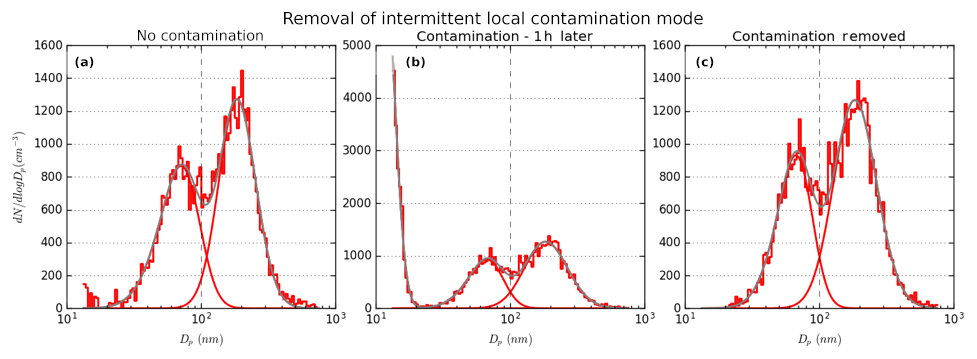
Figure 1 Example removal of intermittent local contamination mode. (a) An observed size distribution with limited impacts from the smallest nucleation mode particles. (b) An observation approximately 1 h later with contamination from small particles that are not representative of the regional aerosol. (c) The same size distribution as in (b), but with the smallest contamination mode identified and removed as described in the text.

2.3 CCN measurements

As described in Martin et al. (2017), size-resolved CCN concentrations (srCCN) were measured using a DMT cloud condensation nuclei counter (CCN-100) coupled with a TSI 3080 SMPS to scan across a range of particle diameters (12–540 nm at water supersaturation of s=0.1 %, 0.19 %, 0.28 %, 0.44 %, 0.58 %, 0.67 %). An apparent hygroscopicity parameter κ (Petters and Kreidenweis, 2007) was calculated from these scans as described in Petters and Petters (2016).

A separate scanning flow CCN system (sfCCN) was used to measure total CCN number concentration as supersaturation was ramped between approximately 0.08 % and 1.1 % supersaturation. The system used a DMT CCN-100 instrument that had been modified by connecting a voltage-modulated proportional flow valve to the bottom of the column to control flow (Suda et al., 2014). The flow rate through the CCN column was increased from 0.2 to 1.2 L min⁻¹ over 5 min while holding the temperature gradient constant, thereby scanning peak column supersaturation as a function of flow rate and column temperature gradient (Moore and Nenes, 2009). A TSI 3010 condensation particle counter (CPC) was placed in parallel to the CCN to measure total particle number concentration (as condensation nuclei, CN). CCN and CN concentrations were recorded at a frequency of 1 Hz. Each approximately 5 min scan was repeated 3 times, after which the temperature gradient was changed to scan a different range of supersaturations. As the column temperatures took approximately 3 min to stabilize, the first scan of each three-repetition set was not analyzed. As the residence time in the sfCCN varied with total flow rate when compared to the parallel CPC, the CPC time stamps were empirically adjusted to ensure the 1 Hz data points from both instruments were aligned, as described in more detail in the Supplement. Calibrations of both CCN systems were conducted following the methodology described in Suda et al. (2012).

Figure 2 Example spectra measured by the sfCCN system for the same time period as in Fig. 1. (a) 1 s CCN (blue) and the range of CN (red) concentration measurements for a single scan. (b) Activated fractions for measured points in (a) along with a best-fit activated fraction spectrum curve (black line). (c, d) As in (a, b), but for a scan approximately 1 h later that was contaminated by an intermittent local ultrafine mode; CN were observed as high as 5000 cm⁻³. (e, f) The same spectra as in (c, d), but after correction to remove the contamination mode; corrected CN concentrations are now similar to the range in (a).

Example sfCCN concentrations (Fig. 2a) and activated fraction spectra (Fig. 2b) are shown for the same time stamp as the size distribution data in Fig. 1. The range of CN concentrations as measured by the parallel CPC during this period are shown via the red background bar. During the contamination period approximately 1 h later the effect of the small mode noted in Fig. 1b was seen via increased CN concentrations (reaching as high as 5000 cm⁻³; Fig. 2c) and decreased activated fractions above approximately 0.1 % supersaturation (Fig. 2d). Observed CCN concentrations remained relatively constant, indicating the additional particles were too small to activate below 1.1 % supersaturation. After removal of this small contamination mode the corrected CN concentrations and activation spectrum (Fig. 2e and f, respectively) were similar in characteristics to the earlier noncontaminated period.

2.4 Classification of aerosol population type

Classification of aerosol population types impacting BML was conducted using an unsupervised K-means cluster analysis. Such clustering methods utilize properties of the aerosol and environment to identify periods of potentially similar impacts and aerosol population types (Wilks, 2011). Cluster analyses have been used to classify aerosol particle size distributions (Tunved et al., 2004), associate them with various environmental and atmospheric processes (Charron et al., 2008; Beddows et al., 2009; Wegner et al., 2012), and conduct aerosol source apportionment studies (Salimi et al., 2014). Information on aerosol chemistry or composition has also been used for clustering purposes (Frossard et al., 2014) and has been integrated with size distribution measurements and atmospheric transport data to produce cluster results based on multiple types of observations (Charron et al., 2008; Atwood et al., 2017).

The K-means clustering methodology involved selection of specific variables that partially defined the state of the aerosol and meteorological environment at the sampling site. The degree of similarity of the state of the environment between any two data points (i.e., specific times) was estimated by the use of a distance function that grouped data points into clusters that had broadly similar values among the input variables. Here, we utilized the cluster.KMeans class of the Python scikit-learn package (Pedregosa et al., 2011) to perform the analysis. Selection of the appropriate number of clusters for the K-means analysis followed a similar methodology to that described in Atwood et al. (2017), and was based on both an initial hierarchical clustering and the use of internal validity measures (Wilks, 2011). First, a hierarchical agglomerative cluster analysis was created using the cluster.AgglomerativeClustering class of scikit-learn to merge the two data points or clusters with the smallest value of the distance function together into a single cluster in subsequent steps until only one cluster remained. A dendrogram was then used to identify potential numbers of clusters at agglomeration steps that had the largest increase in distance between merged clusters. Various internal validity measures of clusters in the ensuing K-means clustering (Beddows et al., 2009; Baarsch and Celebi, 2012) were then used to further assess appropriate numbers of clusters. The final selection of appropriate cluster numbers was based on each of these measures, along with verification that the results maintained physically distinct and temporally coherent clusters, in order to select the appropriate number of K-means clusters.

2.4.1 Cluster variables

A total of 67 clustering variables were used to describe each time stamp in this analysis, which included measurements of aerosol microphysical properties and meteorological parameters at BML. Aerosol property variables included the normalized size distribution (normalized to an integrated value of 1 cm⁻³ by dividing by the total particle number concentration), after correction for local contamination. Values of the normalized number size distributions (dN∕dlog ₁₀D_p) were discretized into 20 logarithmically spaced bins, with each mean bin value then serving as a separate variable in the clustering distance function (e.g., Charron et al., 2008). Similarly, activated fraction spectra (the fraction of particles activated at supersaturation, S) for each time stamp were divided into 20 linearly spaced bins distributed between 0 % and 1.1 % supersaturation to incorporate CCN properties into the analysis. Total particle number concentration was included as a separate cluster variable.

Meteorological parameters at BML included the local 10 m observed wind velocity as perpendicular u and v component variables (two variables). Additionally, HYSPLIT back trajectories were assigned to data points closest in time to each trajectory. The back trajectory was converted to separate variables for the distance function by determining the distance from the receptor, initial bearing, and altitude, every 3 h backwards along the trajectory for 24 h, yielding a total of 24 trajectory clustering variables for each time stamp.

2.4.2 Distance function

As variables of different scale were used in the cluster modeling, the Karl Pearson distance function (Wilks, 2011) was used, wherein each variable is first standardized to ensure they have equal weight on the distance function. However, as the 67 clustering variables were grouped into five categories of measurements (number size distribution, activation spectrum, total particle number concentration, wind speed, and back trajectory), a further modification to the weighting (described below) was used to reduce the impact of differing numbers of variables in these categories on the distance function. The resulting distance between any two data points i and j was given by the function:

$$\begin{array}{}\text{(1)}& {\mathbf{d}}_{i,j}={\left[\sum _{k=\mathrm{1}}^K{\mathit{w}}_k{\left({\mathbf{x}}_{i,k}-{\mathbf{x}}_{j,k}\right)}^{\mathrm{2}}\right]}^{\frac{\mathrm{1}}{\mathrm{2}}},\end{array}$$

where d_i,j gives the distance between two data point vectors, x_i and x_j, in a K-dimensional space (i.e., K nominally independently measured or observed, orthogonal variables at each time stamp), for each variable, k, with weight, w_k, calculated for each variable by the following:

$$\begin{array}{}\text{(2)}& {\mathit{w}}_k={\displaystyle \frac{{\mathit{v}}_k}{{\mathit{s}}_k}},\end{array}$$

where s_k is the variance of the variable k, and v_k is the further relative weight used for each variable.

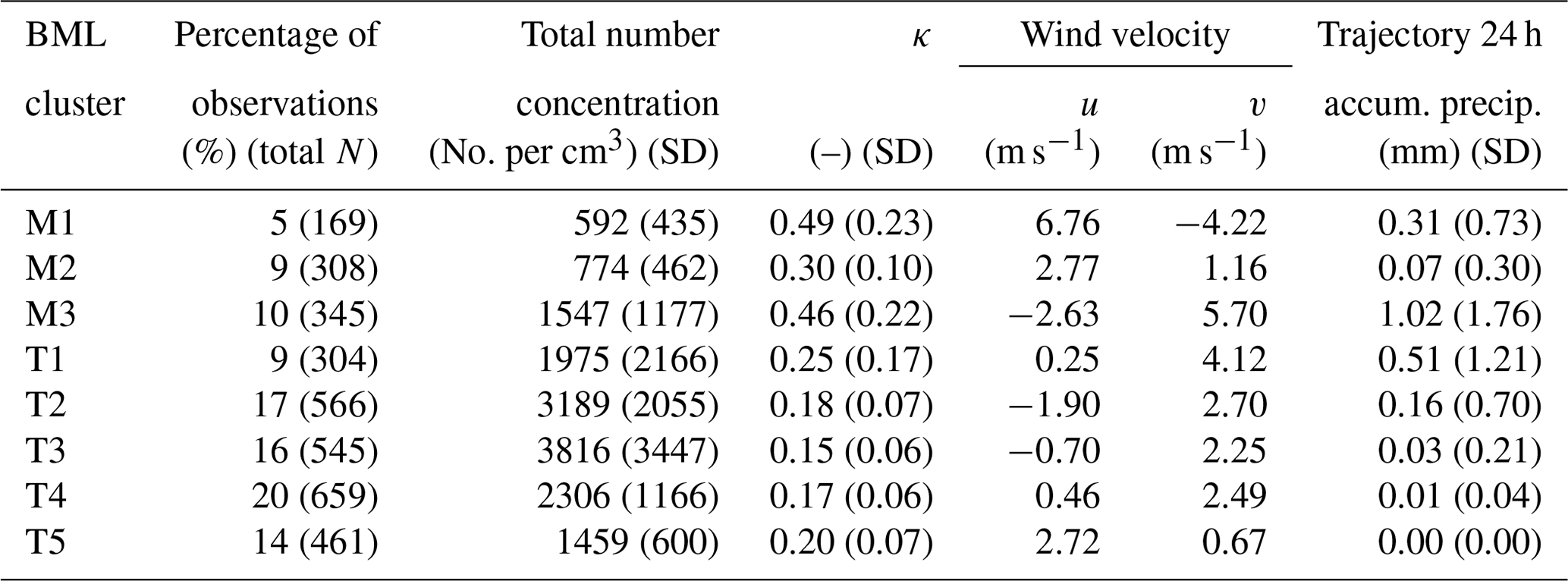
Table 1 Aerosol and meteorological parameters for each of the cluster time periods with the total number and percentage of observations in each cluster. Cluster mean values (and standard deviations where appropriate) are given for total particle number concentration, κ hygroscopicity parameter from the srCCN system, HYSPLIT 24 h accumulated precipitation along the trajectory, and local wind velocity observations.

Only data points with valid measurements for number size distribution and activated fraction were used in the clustering analysis, leaving approximately 94 % of data points (3357 of a total of 3583) utilized. Of the remaining data, two data points had partially invalid activation spectra and were kept in the analysis. The partial spectra had invalid data points imputed to the variable mean to minimize their impact on the distance function.

The size distribution and activated fraction variable categories, each of which had 20 variables, were given relative weights, v_k, of 1∕20 such that their total relative weights summed to 1. As these variables were of primary importance to aerosol population microphysical properties, the other variable groups were decreased in relative importance. The back trajectory and wind vector categories were each assigned a relative weight of 0.5, and the total particle number concentration variable assigned a relative weight of 0.1. As cluster analysis is by its nature an exploratory data analysis technique, these relative weight values were reached by varying their values and assessing the physical interpretability of the results (discussed further in the next section).

2.4.3 Number of clusters

Hierarchical clustering and internal validity measures indicated 2, 6, 8, and 12 clusters were potentially appropriate for the K-means analysis. Clusters associated with periods of marine aerosol impacts (discussed further in the next section) became temporally coherent (i.e., data points assigned to specific clusters tended to occur near each other rather than randomly distributed throughout the study period) and physically meaningful (i.e., could be related to physical phenomena such as land and sea-breeze shifts) after the number of clusters was increased to 8.

In the case of the 12-cluster analysis, several of the clusters were composed of few or even a single data point, indicating the model had begun to separate outliers into distinct clusters. In addition, several of the temporally consistent clusters were split, indicating that too many clusters had been selected. All potential cluster numbers between 7 and 11 were then investigated to determine if physically or temporally coherent population types emerged to a greater degree than the 8-cluster model. The 8-cluster option had been initially identified as potentially appropriate based on the internal validity measures and hierarchical clustering, while other numbers of clusters did not improve results based on the criteria of temporally coherent clusters and physically meaningful interpretation of the cluster results. As such, the 8-cluster model was selected as the most appropriate unsupervised classification result.

3 Aerosol population type classification results and discussion

Three of the eight identified clusters were defined as “marine” population types, as back trajectory data showed evidence of transport pathways primarily over ocean areas. These marine types, denoted as clusters M1–M3, tended to have lower average number concentrations (below approximately 1500 cm⁻³), while the terrestrial clusters (T1–T5) had typical averages between approximately 2000 and 4000 cm⁻³ and were associated with transport from more terrestrial source regions. The exception to this was cluster T5, which had number concentrations of roughly 1500 cm⁻³, more oceanic transport pathways, and size distributions with the largest median diameters among the “terrestrial” clusters. Table 1 provides the cluster-averaged number concentrations, wind velocities, HYSPLIT-accumulated precipitation along the 24 h trajectory, hygroscopicity parameters from the srCCN system, and the percentage of all measurements associated with each of the eight identified clusters. Multi-modal lognormal number size distributions were fit to the average of all spectra associated with each cluster. Fit parameters and best-fit CCN-spectrum activated fraction parameters (see Supplement) for each cluster are provided in Table 2.

Table 2 Cluster best-fit number size distribution and activated fraction parameters are shown, with activated fraction parameters a, b, and c pertaining to the fit model equation given in the Supplement. Clusters with “M” and “T” names refer to marine and terrestrial aerosol population types, respectively.

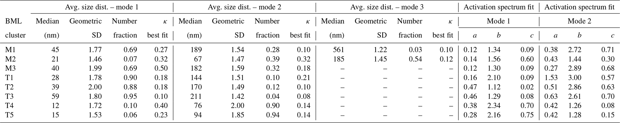
Figure 3 presents the study timelines of measured aerosol (panel a), and meteorological variables (panel b), and the corrected (panel c) and normalized (panel d) aerosol size distributions. The fitted modal diameters are superimposed on the normalized number size distributions, revealing periods of stability in the size distributions as well as periods that are highly variable. Time periods associated with each cluster are shown as colors in the background of the panels.

Changes between identified cluster types often tracked diurnal changes in wind direction associated with the land and sea-breeze cycle (Fig. 3b; e.g., 28–30 January). Several periods occurred during the study during which this diurnal cycle collapsed and BML was ventilated with air masses from marine regions for several days at a time (starting on 4, 17, and 26 February). Clusters M1, M2, and M3 were selected by the model more consistently during these extended periods and confirmed their characterization as marine aerosol population types.

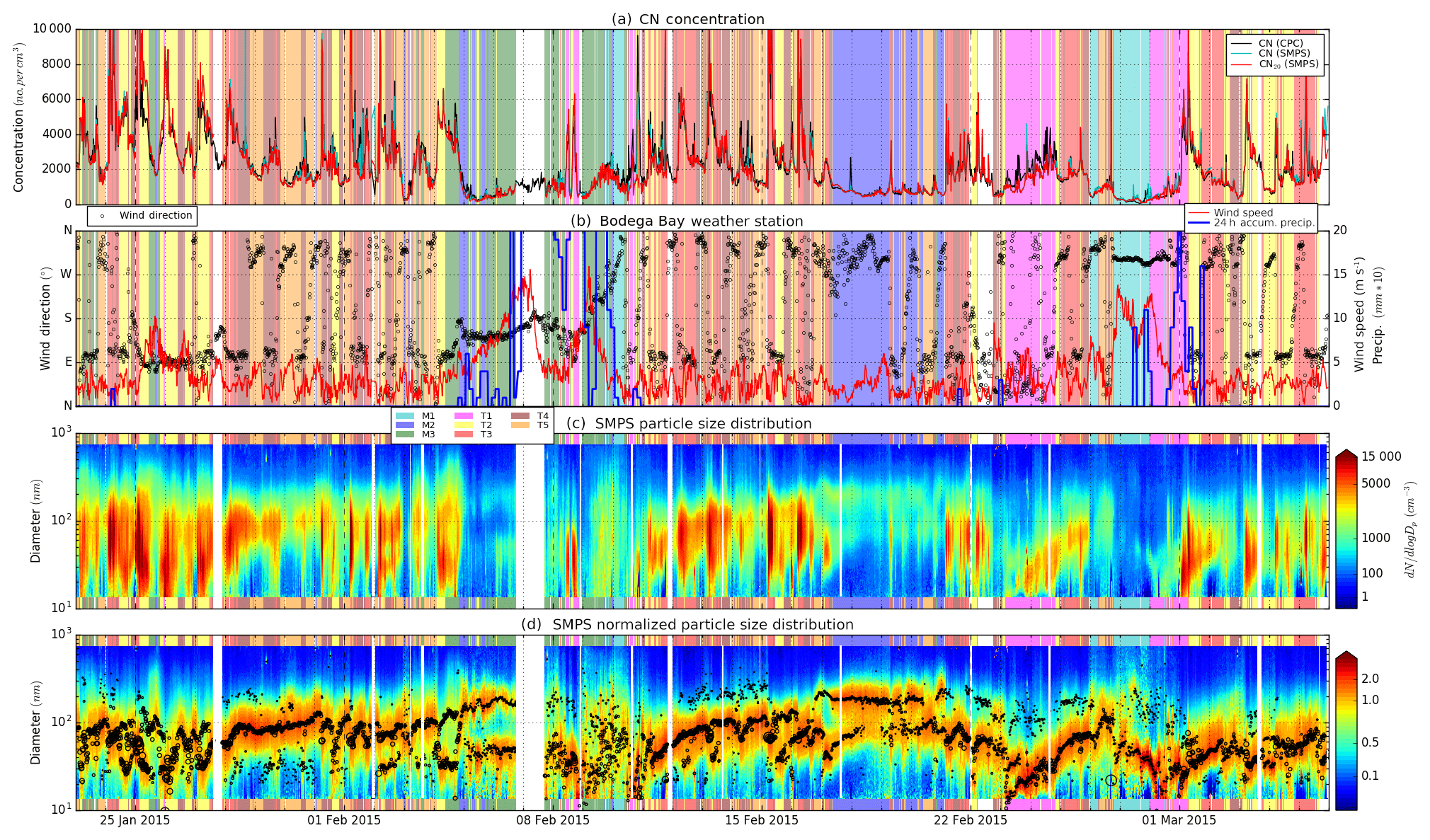
Figure 3 Timelines of study data; all times shown are UTC. (a) Total particle number concentration at BML measured by the CPC (black), reconstructed from SMPS size distributions (blue), and after correction for removal of local sources (red). (b) BML weather station measurements of wind direction (black circles) and wind speed (red lines), with HYSPLIT 24 h accumulated precipitation along the air mass trajectory (blue). (c) SMPS size distribution as dN∕dlog ₁₀D_p and (d) normalized size distributions with best fit median diameters (black circles) with the size of the circle proportional to the number of particles in the mode. Colored backgrounds in each panel are shown for time periods classified as each cluster type for the 8-cluster K-means classification.

Normalized size distributions for the eight clusters are shown in grey in Fig. 4, along with the average total corrected particle number concentrations and the total number of data points included in each cluster. Clusters with terrestrial and/or anthropogenic influence were ordered by increasing median diameter of the mode with the largest number fraction. HYSPLIT back trajectories and wind rose plots for each data point included in each cluster are shown in Fig. 5.

3.1 Marine population types

Further analysis of the marine clusters showed generally distinct meteorological conditions associated with each. Cluster M1 primarily occurred toward the end of the study period, during a period of high-velocity winds from the northwest. Back trajectories agreed with local winds and showed generally faster transport velocities. This cluster dominated during 26 and 27 February, a period during which the cleanest air masses and lowest number concentrations of the study were observed, reaching as low as 50 cm⁻³ during the height of the event. The normalized size distributions indicated that the Aitken mode dominated the number distribution (Fig. 4) and also suggested the presence of a somewhat larger mode (particles larger than ∼ 400 nm) that may have been associated with generation of sea spray by the higher wind velocities. Back trajectories indicated that air masses had passed over the ocean to the northwest of BML, while 24 h accumulated precipitation along the trajectories (Table 1) indicated rainfall had occurred in the days prior to the air mass' arrival at BML. Each of these findings was consistent with classification of the M1 cluster as a precipitation-scrubbed, clean marine aerosol population.

The marine cluster with the next highest number concentration was M2, with 78 % of its total occurrences between 17 and 21 February. The wind rose for this cluster indicated a primarily northwesterly wind, similar to cluster M1 but with much slower velocities, and back trajectories with oceanic transport pathways. While HYSPLIT does not always simulate sub-synoptic-scale transport with high fidelity, this pattern may be indicative of slower transport of air from a marine region just off the coast, as opposed to the direct fast-transport path from more distant ocean regions seen in the M1 type. As observed for M1, the best-fit average normalized particle size distribution (Fig. 4) was primarily bimodal, consistent with many reports of cloud-processed background marine aerosol populations (Hoppel et al., 1986; Bates et al., 2000; Wex et al., 2016; Atwood et al., 2017; Royalty et al., 2017; Phillips et al., 2018), though with a larger accumulation mode number fraction than the M1 type. Minimal rainfall along the transport pathway was evident in the HYSPLIT accumulated precipitation estimates (Table 1), indicating no recent precipitation scrubbing and suggesting that more cloud processing without rainout led to larger numbers of particles in the accumulation mode compared with M1. In contrast to M1, for which a third fitted mode was found above 400 nm, the third mode in M2 occurred at very small particle sizes (diameters less than 30 nm).

The final marine cluster, M3, shared similarities with the other marine types, including a bimodal normalized size distribution with a minimum near 110 nm and indications of oceanic source regions in local winds and back trajectories. However, the average total number concentration was nearly double that of the other marine types. The primary period during which this cluster occurred was during 4–9 February, bracketing the time before, during, and after landfall of the AR that impacted the BML region during CalWater-2015. This cluster is therefore interesting as it may be indicative of a unique population type associated with AR meteorological conditions. Some caution is warranted, however, as instrument downtime lead to a gap in the aerosol size distribution dataset during late 6 February through 7 February, during a high-wind and heavy-precipitation period that marked the landfall of the AR, and thus some key data that could be used to guide the clustering during this event were missing. When confined to the 5–8 February period noted by Leung (2016) when the AR made landfall at BML, the average number concentration was 749 cm⁻³ for time periods associated with the M3 cluster (excluding the data gap on 6–7 February), and 1052 cm⁻³ for the entire 5–8 February AR period (including the intermittent periods classified as terrestrial or anthropogenic aerosol).

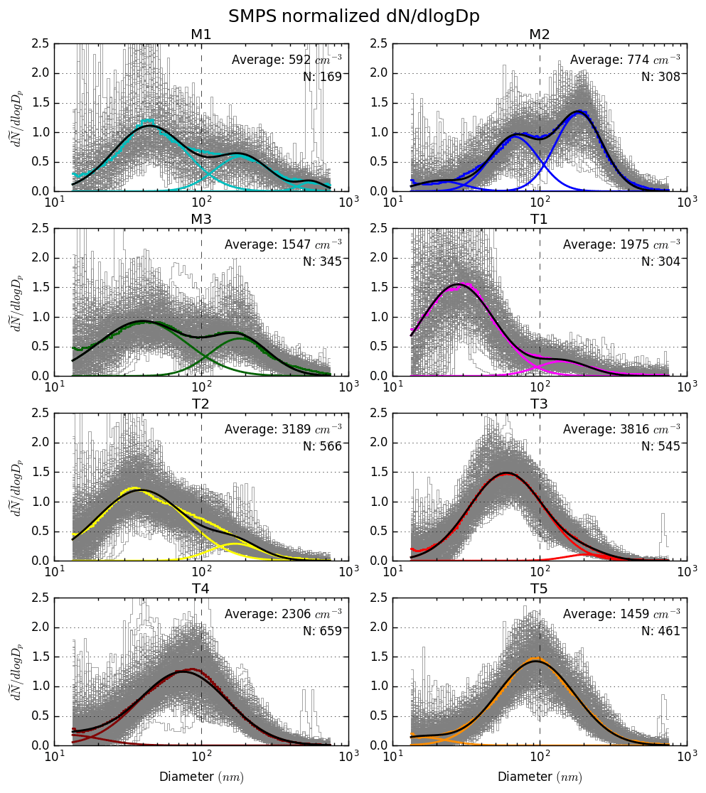
Figure 4 Normalized size distribution for each cluster from the eight-cluster K-means classification. Colored step lines show the average distribution, with best-fit multimodal lognormal fit in black and each mode as colored curves. Observed spectra for each data point in the cluster are shown in grey. Average cluster total particle number concentration and number of data points in each cluster are shown.

Back trajectories for the M3 cluster indicated source regions from just off the coast of the San Francisco Bay area prior to reaching BML, while HYSPLIT accumulated precipitation along the trajectory was the highest of any cluster (Table 1). Flows associated with AR landfall at the coast can be complex (Neiman et al., 2013); however, emissions from this urban area could potentially have mixed with the relatively low particle number counts that would be expected in a precipitation scrubbed AR air mass as it made landfall, accounting for the elevated (> 1000 cm⁻³) total number (CN) concentrations that persisted for much of the AR, including during the high-wind and heavy-precipitation period (Fig. 3b) when SMPS and CCN data were not available. However, local generation of fine-mode sea spray aerosol could also be a factor during high winds.

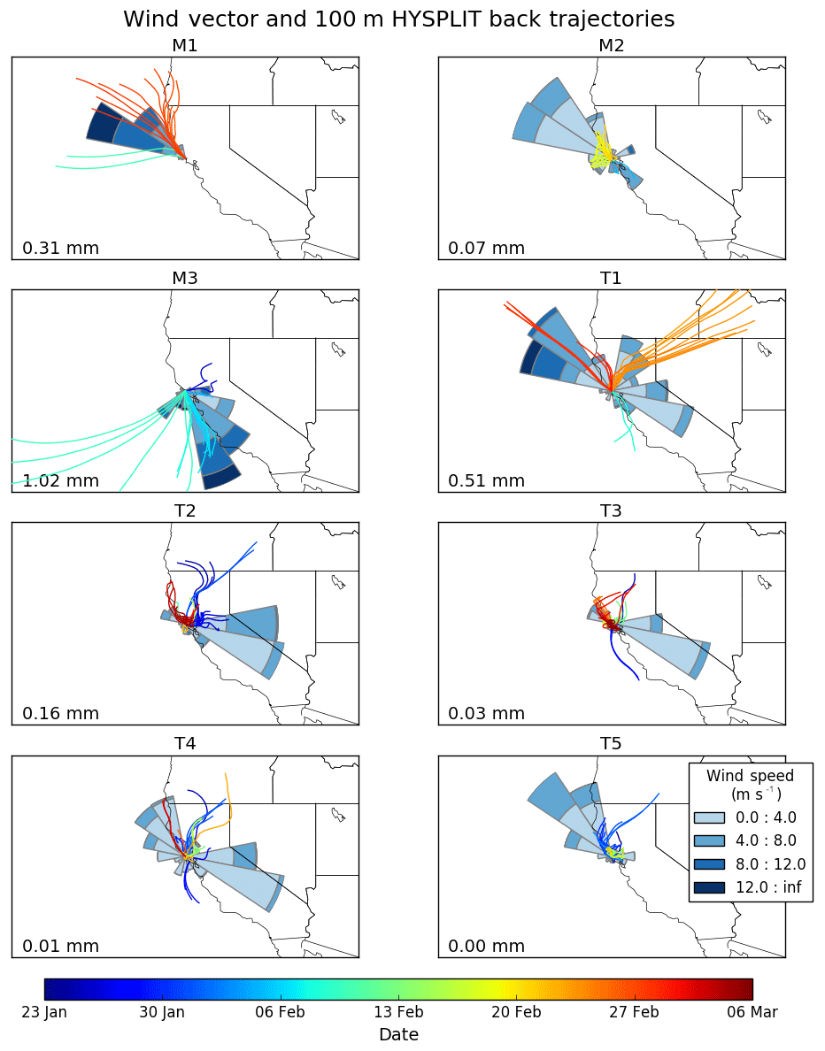
Figure 5 Meteorological overview for each cluster from the eight-cluster K-means classification. HYSPLIT 24 h back trajectories are shown for each time stamp associated with the cluster and colored by the date of arrival at the receptor. Wind rose plots are shown for all BML local 10 m wind direction and velocity measurements for each time stamp associated with the cluster. Mean values for 24 h accumulated precipitation along the trajectory are included in the lower left for each cluster.

3.2 Terrestrial population types

During periods dominated by diurnal shifts in aerosol and meteorological observations, and for short-duration periods during times associated primarily with marine clusters, the cluster model identified clusters that corresponded to terrestrially influenced populations. In the case of the multi-day events dominated by the M1 and M2 types, these short duration periods were often identified as either T4 or T5, clusters that were notable for having largely monomodal normalized size distributions with median diameters around 100 nm. Occurrences of these cluster types were often associated with a spike in number concentration and changes to either wind direction or wind velocity. Thus, the cluster model was able to identify and separate short duration periods of impacts from terrestrial sources during multi-day marine aerosol conditions at BML.

Several longer periods (28–31 January and 13–16 February) were observed during which populations T4 and T5 regularly alternated in tandem with the diurnal land and sea-breeze shift. Similar diurnal-shift behavior, but between clusters T2 and T3, occurred during 25–28 January and 1–5 March. During these diurnal shifts between various terrestrial clusters, the cluster with the larger median diameter was typically associated with the sea breeze and transport from oceanic regions, while the smaller diameter cluster was associated with the land-breeze and transport from terrestrial regions. As aging of terrestrial aerosol typically leads to an increase in the median diameter of the aerosol modes, these four clusters may therefore be indicative of various degrees of aging of regional terrestrial aerosol during “sea-breeze resampling” at BML (Martin et al., 2017). Resampling occurs when terrestrial and marine aerosol populations mix and flow across the coastal boundary at low levels, leading to a region of mixed aerosol populations wherein the larger number concentrations associated with terrestrial types dominate the observed number concentrations in the resulting littoral zone air mass. When this diurnal cycle collapsed and BML was subjected to extended periods of sea breezes and ventilation by air masses almost exclusively from ocean regions, the cluster model selected marine cluster types, indicative of marine air masses that had not experienced much mixing with terrestrial air masses.

The terrestrial type T1 featured a dominant mode of particles with median diameters around 30 nm, indicating relatively little aging of the particles had occurred. Both low-level winds and back trajectories during this cluster type indicated transport pathways from many directions (Fig. 5), though with the highest wind speeds of the terrestrial clusters, consistent with less time between the aerosol source and observation at BML. This cluster occurred primarily during two periods, 23–24 February and 28 February–1 March. During these times, normalized size distributions and modal median diameter fits shown in Fig. 3 indicated that the size distributions associated with the T1 cluster grew over the course of several days into distributions with larger median diameters, which were then classified as other terrestrial cluster types. The T1 cluster may therefore identify a freshly emitted population type or a recent new particle formation event.

3.3 CCN and activated fraction spectra characteristics

The best-fit activated fraction spectra, as functions of water supersaturation, are shown for all valid data points in each of the clusters in Fig. 6a. As a general comparison against other reported values for aerosol activation spectra, Fig. 6 also shows the parameterized spectra reported by Paramonov et al. (2015) for a range of measurement locations from the European EUCAARI Network (grey background) and an overall typical average value (black line). The EUCAARI activation spectra were drawn from a range of marine, littoral, and continental sites and were impacted by both marine and terrestrial air masses, subject to a variety of emissions. The BML spectra spanned much of the range reported for the EUCAARI network, with the M2 cluster slightly above this range at intermediate supersaturations. Activated fraction spectra are independent of total number concentration, thus the effect of particle size on activation is evident for the BML cases, with clusters with larger size modes having higher activated fractions across the range of measured supersaturations. These results show the wide range of activated fraction spectra at BML associated with differences in aerosol population type, and the corresponding complexity of the population characteristics at this site.

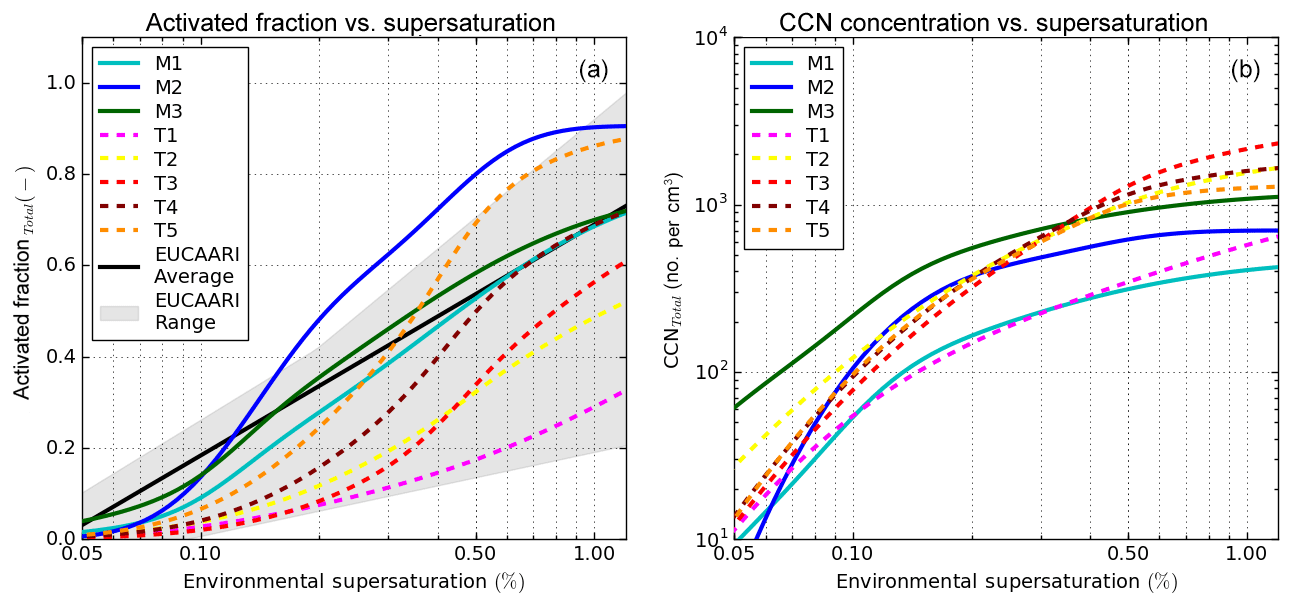
Figure 6 (a) Best-fit activated fraction spectra for each cluster in the eight-cluster K-means analysis, with marine aerosol population types plotted as solid lines, and terrestrial clusters types as dotted lines. Cluster average spectra are compared against the maximum and minimum values (grey shading) and overall average (black line) reported by Paramonov et al. (2015) from a range of sampling locations in the European EUCAARI network. (b) Parameterized mean CCN concentrations across the same range of supersaturation values for each cluster in the eight-cluster K-means analysis.

In the CalWater-2015 dataset, marine population types all reached activated fractions of about 0.2 at supersaturations around 0.1 % to 0.15 %, while the terrestrial types did not reach equivalent fractions until supersaturations between approximately 0.18 % and 0.6 % were reached. Terrestrial population types with smaller median diameters tended to have less fractional activation across the full range of measured supersaturations, leading to activated fractions at 1.0 % supersaturation that varied from approximately 0.3 to 0.85. However, due to the generally higher total particle number concentrations, and despite lower activated fractions of the terrestrial populations, differences in CCN concentrations between marine and terrestrial types (Fig. 6b) were smaller than the differences in the activated fraction spectra. Only at supersaturations above approximately 0.5 % did the CCN concentration for the terrestrial types (except T1, associated with many fresh, small particles) consistently exceed those of the marine types (Fig. 6b). Between approximately 0.1 % and 0.4 %, CCN concentrations were often similar between the marine and terrestrial types.

3.4 Comparison of reconstructed and directly measured CCN spectra

Average values for observations of the hygroscopicity parameter κ from the srCCN system are given for each cluster in Table 1. Mean κ values for the three marine population types were higher than for any of the terrestrial clusters, with the κ for the marine populations found to be significantly different (p<0.05) from those for any of the terrestrial clusters.

Mean measured κ values of 0.49 and 0.46 for the M1 and M3 population types, respectively, were within the range of mean κ values (0.30–0.54) for marine-aerosol-dominated periods in a coastal outflow marine region presented by Phillips et al. (2018). Mean values for terrestrial population types T1–T5 varied between 0.15 and 0.25 and were consistent with the 0.20 value for Aitken mode continental outflow aerosol reported by Phillips et al. (2018). However, we note that κ values measured in this study and used in the closure calculations were derived from supersaturated CCN measurements, whereas Phillips et al. (2018) reported κ from humidified growth factors at 80 % RH. Prior work has shown that κ is not always consistent across this large of a span of RH (Irwin et al., 2010; Whitehead et al., 2014), thus contributing to uncertainty in such comparisons. The hygroscopicity for the final marine M2 type was 0.30, near the lower end of typical values for marine aerosol in regions of continental outflow, but still above those of the terrestrial population types. As the M2 cluster was also the only marine population type with no indication of recent precipitation scrubbing of the air mass prior to arrival at BML (Fig. 3b), some combination of influences from cloud processing, marine, and terrestrial or anthropogenic sources may result in the observed hygroscopicity values between those of the other population types.

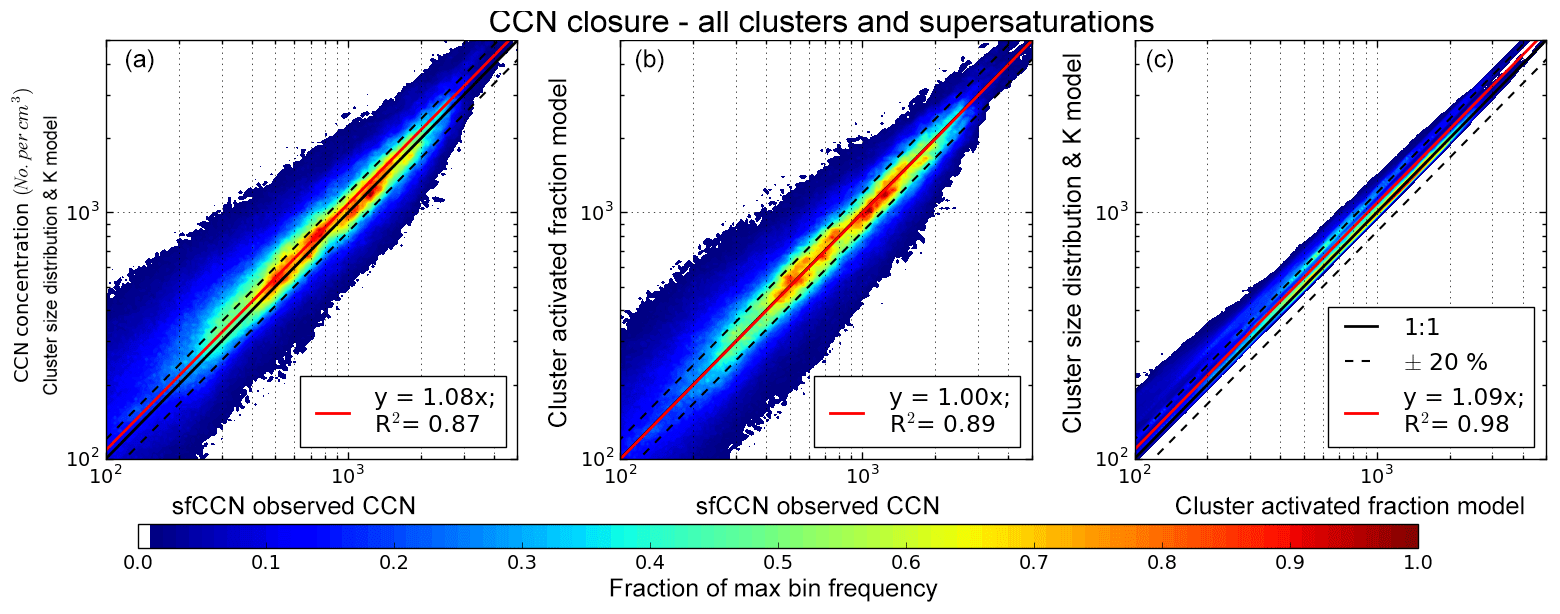
Figure 7 CCN closure comparing predicted and measured CCN number concentrations for (a) the predicted concentration based on the size distribution and κ reconstruction against observed concentrations, (b) the predicted concentration based on the best-fit activated fraction reconstruction against observed concentrations, and (c) the comparison between the two reconstruction methods. All cluster types and supersaturations across the full range of observed values are shown. Linear best-fit slope is shown in red with the associated R² values. One-to-one lines and lines at ±20 % are shown. Colors represent the data point density as a fraction of the maximum density in each plot.

The cluster-average hygroscopicities from Table 1 were combined with the average cluster size distributions from Table 2 to create a reconstructed activated fraction spectrum for each cluster. These reconstructions are compared with the direct-measured CCN spectra in Fig. S3 and Table 2. Generally, the reconstructed spectra are within 1 standard deviation of the directly measured spectra from the sfCCN system. However, the reconstruction overpredicts activated fraction for the marine clusters, with the largest discrepancies at low supersaturations and low CCN number concentrations. Similar behaviors in overprediction of CCN concentrations based on reconstructions using hygroscopicity and size distributions have been noted before (McFiggans et al., 2006). Kammermann et al. (2010) reviewed a number of studies that compared such predicted CCN concentrations against observed values and found biases were often largest at supersaturations below 0.3 %, where predictions deviated from observations by factors ranging from 0.6 to 3.3, with most studies finding overprediction occurred. They attributed the increasing bias at decreasing supersaturations to increased uncertainty in the critical activation diameter and associated CCN number prediction, though they also noted that this discrepancy between predicted and observed CCN concentrations has not been fully resolved. At larger particle diameters measurement uncertainty increases due to imprecise particle size cuts, losses in inlets and tubing, and inversion uncertainties, along with generally lower number concentrations than at smaller particle diameters, leading to higher expected uncertainty in CCN predictions and reconstructions when the critical activation diameter is in this range of particle sizes. At low supersaturations where BML data showed an overprediction bias the critical activation diameter would be above 150 nm. The marine types that had the largest biases at low supersaturations also tended to have larger fractions of particles at these large sizes. This would be expected to add to uncertainty in ways similar to those noted by Kammermann et al. (2010) and potentially explain the larger discrepancies in CCN prediction at lower supersaturations in the marine aerosol types.

Further investigation of the closure between predicted and observed CCN concentration was conducted using two prediction models. Hygroscopicity-derived predictions using cluster average κ and normalized size distribution values were generated and compared against all observed CCN concentrations by the sfCCN system in Fig. 7a. Similarly, the predicted CCN concentrations using cluster average activated fraction spectra were compared against observations in Fig. 7b. Both models predicted the activated fraction using the cluster type identified during the observation, which was then multiplied by the observed total number concentration at the observation time. The hygroscopicity and size model showed overprediction compared to both observations and the activated fraction model (Fig. 7c), with best-fit slopes of 1.08 and 1.09 respectively. The activated fraction model predictions did improve on the hygroscopicity model, with a slope of 1.00 and R² values increasing from 0.87 to 0.89, though this is in part due to the model being based on a direct fit of the observed data. Nevertheless, the degree of closure between model predictions and observed CCN concentrations is similar to closures previously reported in field studies (e.g., Bougiatioti et al., 2009; Kammermann et al., 2010).

3.5 Aerosol optical properties

While optical properties of the various aerosol population types were not directly measured, a simple optical reconstruction was conducted to evaluate potential differences between the population types due to differences in size distribution and hygroscopicity. Average particle size distributions and measured average κ values were used to grow particles to equilibrium with relative humidity across a range of values between 0 % and 99 %, assuming deliquesced particles, followed by estimation of mass scattering efficiency on a dry aerosol mass basis using Mie theory (Bohren and Huffman, 1983). For the purposes of this simple optical comparison, supersaturated κ values used for this analysis were assumed to be sufficient to provide an estimate of subsaturated hygroscopic growth. The average size distribution for each aerosol population type was assumed to be made for a deliquesced aerosol at the study average SMPS-measured RH of 35.5 % (Martin et al., 2017) and the cluster average κ given in Table 1. An assumed dry index of refraction of 1.5+0.0i and density of 1.0 g cm⁻³ (e.g., Remer et al., 2006) were used for all population types in order to estimate the relative effect of differences in size distribution, hygroscopicity, and relative humidity on scattering properties at a wavelength of 550 nm. The index of refraction of each humidified particle was adjusted based on volume mixing with water ($m=\mathrm{1.33}+\mathrm{0.0}i$). Reconstructed mass scattering efficiencies for each of the population types are shown in Fig. 8.

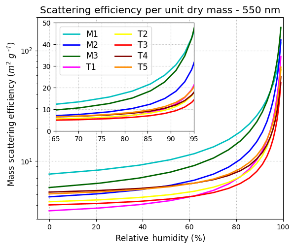
Figure 8 Reconstructed mass scattering efficiencies (per unit dry aerosol mass) for each of the cluster population types across a range of environmental relative humidity values. An assumed dry index of refraction of 1.5+0.0i was used for all population types to highlight the differences in aerosol optical properties expected due to differences in population average size distribution, hygroscopicity, and relative humidity.

Mass scattering efficiencies at 550 nm for particles modeled at 0 % RH ranged between 3.6 and 7.6 m² g⁻¹, although actual values would be expected to be lower due to expected particle dry densities higher than 1 g cm⁻³. Further, these values represent only the contribution to mass scattering efficiencies from fine-mode aerosol. Coarse-mode aerosol, including particles generated by sea spray in littoral environments, can represent a large fraction of the total light scattering, although their mass scattering efficiencies are typically lower. The M1 and M3 marine types, which included the largest fraction of larger accumulation mode particles, had the highest associated dry mass scattering efficiency. The M2 marine type, which occurred at generally lower wind speeds than the other marine types and thus had fewer larger particles associated with wind-generated sea spray aerosol (O'Dowd and Leeuw, 2007), had a lower dry mass scattering efficiency than several of the terrestrial types with the largest median particle diameters. However, at relative humidity values above roughly 60 %, as would typically be expected in littoral environments such as BML, the marine population types all yielded expected mass scattering efficiencies above those of the terrestrial types. For the marine types at a relative humidity of 95 %, the mass scattering efficiencies on a unit-density dry mass basis were between 31 and 47 m² g⁻¹, roughly twice the range of the terrestrial types, 14 to 21 m² g⁻¹.

4 Summary

The unsupervised cluster model analysis successfully identified distinct aerosol population types in the littoral zone aerosol at BML during CalWater-2015. The time periods selected by each cluster tended to be both temporally and physically coherent. Clusters also tended to be grouped into periods with physically meaningful microphysical properties that could be associated with meteorological processes and expected sources and transport pathways. For example, the clustering methodology identified regular diurnal swings in aerosol properties associated with land and sea-breeze changes and assigned two distinct, terrestrially influenced aerosol types during these periods. Overall, the clustering results for the CalWater-2015 dataset produced a reliable set of aerosol population types and appropriately screened intermittent periods of impacts from various other sources as an outcome of the classification. Both marine and terrestrially influenced aerosol population types were identified by the unsupervised cluster model. Several marine events that persisted for days were identified as distinct in character from each other – differing in the degree of cloud processing and precipitation removal prior to arrival at the measurement site, and in the extent to which high winds contributed larger sea spray particles. About 10 % of the observations were associated with a terrestrial population with a large fraction of small particles, indicating it was affected by relatively fresh emissions and/or new particle formation.

A primary motivation for CalWater-2015 was improving characterization of the regional aerosol and how it might affect the formation of precipitation. The CCN activation spectra observed at BML spanned a full range reported in the literature, from clean marine to strongly terrestrially influenced in character. However, differences in total aerosol number concentrations associated with the marine and terrestrial types partially offset the differences in activated fraction over a range of measured supersaturations, such that the variability in CCN concentrations between some marine and terrestrial aerosol types at some supersaturations was less than expected from the differences in the averaged total aerosol particle concentrations.

In this littoral region sea-breeze resampling and complex mixing between marine, terrestrial, and free-tropospheric air masses lead to complex aerosol populations. Determination of which aerosol types can become incorporated into AR events and thereby affect cloud and precipitation over California depends strongly on the individual nature of the flow regimes and potential aerosol source regions that they tap into. Nevertheless, the observational dataset had cases for which marine and terrestrial CCN concentrations were comparable at supersaturations below approximately 0.4 %, and thus changes in aerosol types would result in little change to initial drop populations in the resulting stratus cloud, except at very low supersaturations. Thus, mixed-phase microphysical processes occurring in those clouds might also be expected to be similar whether marine or terrestrial aerosols served as the nuclei for the supercooled droplets. In contrast, for clouds forming at higher maximum supersaturations, terrestrial aerosol populations are expected to yield higher drop concentrations than marine types, with the exception of a terrestrial population characterized by primarily small, recently emitted, or newly formed particles. Thus the droplet size distributions formed on terrestrial vs. marine types, for liquid clouds formed in stronger updrafts or at higher cooling rates that reach such higher supersaturations, should be distinctly different.

At the BML observational site, apparent aerosol types changed over much shorter timescales than a multi-day classification based on prevailing meteorological conditions would suggest, consistent with complex flows in coastal zones. Inclusion of both meteorological and aerosol properties into the schemes used in unsupervised cluster models therefore yielded improvements in the classification of aerosol and air mass types observed at the surface and successfully identified changes at time resolutions on the order of hours. Further work on the classification of aerosol populations in complex or highly variable regions may therefore benefit from the inclusion of a wider range of measurements or observed properties into clustering methods.