Receptor modelling of both particle composition and size distribution from a background site in London, UK – a two-step approach

Some air pollution datasets contain multiple variables with a range of measurement units, and combined analysis using positive matrix factorization (PMF) can be problematic but can offer benefits through the greater information content. In this work, a novel method is devised and the source apportionment of a mixed unit dataset (PM₁₀ mass and number size distribution, NSD) is achieved using a novel two-step approach to PMF. In the first step the PM₁₀ data are PMF-analysed using a source apportionment approach in order to provide a solution which best describes the environment and conditions considered. The time series G values (and errors) of the PM₁₀ solution are then taken forward into the second step, where they are combined with the NSD data and analysed in a second PMF analysis. This results in NSD data associated with the apportioned PM₁₀ factors. We exemplify this approach using data reported in the study of Beddows et al. (2015), producing one solution which unifies the two separate solutions for PM₁₀ and NSD data datasets together. We also show how regression of the NSD size bins and the G time series can be used to elaborate the solution by identifying NSD factors (such as nucleation) not influencing the PM₁₀ mass.

1 Introduction

It is unquestionable that worldwide, the scientific vista of air quality is expanding, whether it is the increasing number of observatories or the refinement of information mined from the increasing sophistication of measurements often incorporated in campaign work. The number of metrics being measured has increased from simple measurements of particulate matter (PM) mass and gas concentrations, and we can now probe the composition of the PM mass and the size distributions with mass spectrometers, mobility analysers and optical devices.

Studies using positive matrix factorization (PMF) as a tool for source apportionment of particle mass using multicomponent chemical analysis data are published frequently using datasets from around the world. However, they do not always provide consistent outcomes (Pant and Harrison, 2012), and one means by which source resolution and identification can be improved is by inclusion of auxiliary data, such as gaseous pollutants (Thimmaiah et al., 2009), particle number count (Masiol et al., 2017) or particle size distribution (Beddows et al., 2015; Ogulei et al., 2006; Leoni et al., 2018).

Harrison et al. (2011) analysed number size distribution (NSD) data (merged Scanning Mobility Particle Sizer (SMPS) and Aerodynamic Particle Sizer (APS) data) with PMF using auxiliary data (meteorology, gas concentration, traffic counts and speed). The study used particle size distribution data collected at the Marylebone Road supersite in London in the autumn of 2007 and put forward a 10-factor solution comprised of roadside and background particle source factors. Sowlat et al. (2016) carried out a similar analysis on number size distribution (13 nm–10 µm) data combined with several auxiliary variables collected in Los Angeles. These included black carbon (BC), elemental carbon (EC) and organic carbon (OC), PM mass, gaseous pollutants and meteorological and traffic flow data. A six-factor solution was chosen comprising of nucleation, two traffic factors, an urban background aerosol, a secondary aerosol and a soil factor. The two traffic sources contributed up to above 60 % of the total number concentrations combined. Nucleation was also observed as a major factor (17 %). Urban background aerosol, secondary aerosol and soil, with relative contributions of approximately 12 %, 2.1 % and 1.1 %, respectively, overall accounted for approximately 15 % of PM number concentrations, although these factors dominated the PM volume and mass concentrations, due mainly to their larger mode diameters. Chan et al. (2011) considered extracting more source information from an aerosol composition dataset by including data on other air pollutants and wind data in the analysis of a small but comprehensive dataset from a 24-hourly sampling programme carried out during June 2001 in an industrial area in Brisbane. They chose multiple types of composition data (aerosols, volatile organic compounds (VOCs) and major gaseous pollutants) and wind data in source apportionment of air pollutants and found it to result in better defined source factors and better fit diagnostics, compared to when non-combined data were used. Likewise, Wang et al. (2017) report an improvement in source profiles when coupling the PMF model with ¹⁴C data to constrain the PMF run as a priori information.

However, while combining, for example, particle chemical composition and size distribution data in a single PMF analysis may assist source resolution, difficulties arise if the two datasets have different and/or ambiguous rotations (discussed in Sect. 2). This tends to result in factors with either mass contributions and small number contributions or number contributions and small mass contributions and rarely a meaningful contribution from both data types. Experimental design can of course circumnavigate this problem, for instance, using chemical data which are already size-segregated, measured using a cascade impactor (Contini et al., 2014). Such an approach is attractive by view of the fact that there is no question as to whether both datasets sufficiently overlap across the size bins. However, cascade impactors do not offer the high time resolution of particle counting instruments, with individual measurements lasting hours or days. Even so, for the case in which two or more instruments are available in a campaign to measure two or more different metrics, e.g. PM mass and particle number (PN), then a combined data analysis is useful. Emami and Hopke (2017) have shown that the effect of adding variables as auxiliary data (with potentially different units) to a NSD dataset is to decrease the rotational ambiguity of a solution from a one-step PMF analysis.

In this study, we present a method for analysing simultaneously collected PM₁₀ composition and NSD data. In the work of Beddows et al. (2015), both particle composition and NSD data from a background site in London (2011 and 2012) were analysed using positive matrix factorization. As part of the methodology development, it was concluded that it was preferable not to combine these two data types in a single analysis but to conduct separate PMF analyses for PM₁₀ mass and particle number. This yielded a six-factor solution for the PM₁₀ data (diffuse urban, marine, secondary, non-exhaust traffic and crustal (NET and crustal), fuel oil and traffic). Factors described as diffuse urban, secondary and traffic were identified in the four-factor solution for the NSD data, together with a nucleation factor not seen in the PM₁₀ mass data analysis (see Fig. 1). When combining the PM₁₀ and NSD data in a single PMF analysis, diffuse urban, nucleation, secondary, aged marine and traffic factors were identified, but the factors were not as clearly separated from each other as the factors derived from the separate datasets. For example, fuel oil was now mixed in with marine and called aged marine. This is summarized in Fig. 1. However, it would still be useful to obtain a number size distribution for each of the six PM₁₀ factors and/or a chemical composition for the four NSD factors. As a continuation of this work, we present an alternative method for analysing the combined dataset in a so-called two-step methodology. In the first step, we analyse the mass data (PM₁₀; units: µg m⁻³) according to the methodology of Beddows et al. (2015). This results in a time series factor G, which is carried forward into a second PMF analysis of a combined dataset consisting of the G time series and an auxiliary dataset (i.e. NSD; units: cm⁻³). The first step identifies sources and apportions the G factors to their contribution to mass, and in the second step, an FKEY matrix is chosen such that G “drives” the model and the NSD data “follow”. This means that we have PM₁₀ factors, each of which is augmented by its number size distribution. Furthermore, we also consider linear regression (LR) as a second step in a PMF–LR analysis to show that although the initial analysis is biased toward mass by analysing PM₁₀ factors only, unseen factors influencing the NSD data (e.g. nucleation) can be identified in the data.

Figure 1 Venn diagram showing the summary of the findings of Beddows et al. (2015), applying PMF to PM₁₀-only, NSD-only and PM₁₀–NSD datasets. Table shows the apportionment of PM₁₀ and NSD taken from Beddows et al. (2015).

2 Experiment

With a population of 8.5 million in 2014 (ONS, 2017), the UK city of London is the focus of study in this work; the North Kensington (NK) site (lat. = 51^∘: 31^′: 15.780^′′ N and long. = 0^∘: 12^′: 48.571^′′ W) was considered. NK is part of both the London Air Quality Network and the national Automatic Urban and Rural Network and is owned and part-funded by the Royal Borough of Kensington and Chelsea. The facility is located within a self-contained cabin within the grounds of Sion Manning School. The nearest road, St. Charles Square, is a quiet residential street approximately 5 m from the monitoring site, and the surrounding area is mainly residential. The nearest heavily trafficked roads are the B450 (∼100 m east) and the very busy A40 (∼400 m south). For a detailed overview of the air pollution climate at North Kensington, the reader is referred to Bigi and Harrison (2010).

2.1 Data

As alluded to, this work is a continuation of the study carried out by Beddows et al. (2015), which analysed NSD and PM₁₀ chemical composition data collected at the NK receptor site. Number size distribution (NSD) data were collected continuously every 15 min using a Scanning Mobility Particle Sizer (SMPS), consisting of a CPC (TSI model 3775) combined with an electrostatic classifier (TSI model 3080) and air-dried according to the EUSAAR protocol (Wiedensohler et al., 2012). The particle sizes covered were 51 size bins ranging from 16 to 604 nm, the 15 min distributions were aggregated up to hourly averages (when there were at least three 15 min samples per hour) and all missing values were replaced using a value calculated using the method of Polissar et al. (1998). Further details of the SMPS settings are given in Table S1 in the Supplement, and the reader is also referred to Beccaceci et al. (2013a, b) for an extensive account of how the NSD data were collected and quality-assured.

Accompanying the NSD data from the study of Beddows et al. (2015) was the PMF output from the analysis of PM₁₀ chemical composition data. The latter data consisted of 24 h air samples taken daily over a 2-year period (2011 and 2012) using a Thermo Partisol 2025 sampler fitted with a PM₁₀ size-selective inlet. These filters were analysed for total metals, PM_metals (Al, Ba, Ca, Cd, Cr, Cu, Fe, K, Mg, Mo, Na, Ni, Pb, Sn, Sb, Sr, V and Zn), using a Perkin Elmer/Sciex ELAN 6100DRC following hydrofluoric acid digestion of GN-4 Metricel membrane filters. Water-soluble ions, PM_ions (Ca²⁺, Mg²⁺, K, ${\mathrm{NH}}_{\mathrm{4}}^{+}$, Cl⁻, ${\mathrm{NO}}_{\mathrm{3}}^{-}$ and ${\mathrm{SO}}_{\mathrm{4}}^{\mathrm{2}-}$), were measured using a near-real-time URG-9000B (hereafter URG) ambient ion monitor (URG Corp). The data capture over the 2 years ranged from 48 % to 100 % as different sampling instruments varied in reliability. Data gaps were filled by measurements made on daily PM₁₀ filter samples collected continuously at this site using a Partisol 2025; laboratory-based ion chromatography measurements were made for anions on Tissuquartz^™ 2500 QAT-UP filters. No cation measurements were available from these filters, and this resulted in a lower data capture for the cations. Again, all missing data were replaced using a value calculated using the method of Polissar et al. (1998). A woodsmoke metric, CWOD, was also included. This was derived as PM woodsmoke from the methodology of Sandradewi et al. (2008) utilizing aethalometer and EC∕OC data, as described in Fuller et al. (2014). Samples were also collected using a Partisol 2025 with a PM₁₀ size-selective inlet, and concentrations of elemental carbon (EC) and organic carbon (OC) were measured through collection on quartz filters (Tissuquartz^™ 2500 QAT-UP) and analysis using a Sunset Laboratory thermal–optical analyser according to the QUARTZ protocol (which gives results very similar to EUSAAR 2: Cavalli et al., 2010) (NPL, 2013). We refer to CWOD, EC and OC as PM_carbon. In addition, particle mass was determined on samples collected on Teflon-coated glass fibre filters (TX40HI20WW) with a Partisol sampler and PM₁₀ size-selective inlet.

This aforementioned PM₁₀ data were represented in this work as the PMF solution for PM₁₀-only data, derived in Beddows et al. (2015) and consisting of six sources, namely diffuse urban, marine, secondary, non-exhaust traffic and crustal, fuel oil and traffic. The diffuse urban factor had a chemical profile indicative of contributions mainly from both woodsmoke (CWOD) and road traffic (Ba, Cu, Fe, Zn). The marine factor explained much of the variation in the data for Na, Cl⁻ and Mg²⁺, and the secondary factor was identified from a strong association with ${\mathrm{NH}}_{\mathrm{4}}^{+}$, ${\mathrm{NO}}_{\mathrm{3}}^{-}$, ${\mathrm{SO}}_{\mathrm{4}}^{\mathrm{2}-}$ and organic carbon. For the traffic emissions, the PM did not simply reflect tailpipe emissions, as it also included contributions from non-exhaust sources, i.e. resuspension of road dust and primary PM emissions from brake, clutch and tyre wear. The non-exhaust traffic and crustal factor explained a high proportion of the variation in the Al, Ca²⁺ and Ti measurements consistent with particles derived from crustal material, derived either from wind-blown or vehicle-induced resuspension. There was also a significant explanation of the variation in elements such as Zn, Pb, Mn, Fe, Cu and Ba, which had a strong association with non-exhaust traffic emissions. As there was a strong contribution of crustal material to particles resuspended from traffic, this likely reflected the presence of particulate matter from resuspension and traffic-polluted soils. The last factor was attributed to fuel oil, characterized by a strong association with V and Ni together with significant ${\mathrm{SO}}_{\mathrm{4}}^{\mathrm{2}-}$. This output comprised the first-step solution in the two-step analysis of PM₁₀ and NSD data, and in this study we concentrate on the analysis of the NSD data in the second PMF step, with the aim of assigning a NSD to each of the six PM₁₀ factors.

2.2 Methods

2.2.1 PMF

Positive matrix factorization (PMF) is a well-established multivariate data analysis method used in the field of aerosol science. PMF can be described as a least-squares formulation of factor analysis developed by Paatero (Paatero and Tapper, 1994). It assumes that the ambient aerosol concentration X (represented by m×n matrix of m observations and n PM₁₀ constituents or NSD size bins), measured at one or more sites, can be explained by the product of a source profile matrix F and source contribution matrix G whose elements are given by Eq. (1):

$$\begin{array}{}\text{(1)}& {\displaystyle }{x}_{ij}=\sum _{k=\mathrm{1}}^p{g}_{ik}\cdot f_{kj}+e_{ij}i=\mathrm{1}\mathrm{\dots }m;j=\mathrm{1}\mathrm{\dots }n,\end{array}$$

where the jth PM constituent (element, size bin or auxiliary measurement) on the ith observation (i.e. hour) is represented by x_ij. The term g_ik is the contribution of the kth factor (of a total of p factors) to the receptor on the ith hour, f_kj is the fraction of the jth PM constituent in the kth factor and e_ij is the residual for the jth measurement on the ith hour. The residuals (i.e. difference between measured and reconstructed concentrations) are accounted for in matrix E, and the two matrices G and F are obtained using an iterative algorithm which minimizes the object function Q (see Eq. 2).

Using the data and uncertainty matrices for the model, Eq. (1) is optimized in the PMF algorithm by minimizing the Q value (Eq. 2):

$$\begin{array}{}\text{(2)}& {\displaystyle }Q=\sum _{i=\mathrm{1}}^n\sum _{j=\mathrm{1}}^m{\left({\displaystyle \frac{e_{ij}}{s_{ij}}}\right)}^{\mathrm{2}},\end{array}$$

where s_ij is the uncertainty in the jth measurement for hour i. All analyses were carried out in robust mode which reduces the impact of outliers (Paatero, 2002).

PMF is a weighted technique, and the value of Q, and hence the model fit, is determined by the input variables with the lowest values of uncertainty, s_ij, thus giving their variables a higher weighting in the analysis. Input variables with low weight have little effect upon the value of Q, even when their residuals are large. This can be used to the advantage of the operator; e.g. when apportioning total PM mass in a conventional one-step PMF, the total PM concentrations are normally input with artificially high uncertainty, so that they are essentially passive in the PMF analysis and do not influence its outcome. By doing so, the chemical composition data determine the apportionment of PM mass to the source-related factors identified by the PMF. A similar approach can be followed in the PMF analysis of a combined dataset, whereby higher weightings can be applied to the main dataset of interest such that it drives the analysis and the auxiliary dataset follows; i.e. the uncertainties are chosen such that the balance of total weights from the two datasets is tipped towards the measurement of interest and highest reliability in regards of rotational unambiguity.

To assess the PMF model, the Q value is outputted by PMF and compared to a theoretical value Q_theory. which is approximately the difference between the product of the dimensions of X and the product of the number of factors and the sum of dimensions of X (i.e. m×n – p(m+n)). For a given number of factors, the whole uncertainty matrix is scaled by a factor b_scale until the ratio between Q and Q_theory is approximately 1 (rQ value = $Q/Q_{\text{theory}}=\mathrm{1}\pm \mathrm{0.02}$).

With regards to the final output from PMF, a scaling has to be applied in order to achieve quantitative results. This is done by scaling either G or F to unity such that the units from X are carried over to either F or G respectively to complete the apportionment. However, different routes have to be considered depending on whether X has homogeneous or heterogeneous units.

2.2.2 One-step method using data in the same units – homogeneous units

Given a PMF input data matrix X, a solution GF+E can be computed, where G represents the time series of the source profiles F, with a residual matrix E. Often X comprises columns of PM₁₀ component concentrations (e.g. ICPMS values measured from acid-digested filters collected with a Partisol 2025), and it is common practice to also include a total variable (e.g. column of PM₁₀, measured using a Tapered Element Oscillating Microbalance, TEOM) in the data matrix. The resulting PM₁₀ profile element value can then be used to scale G and F such that G carries the units of X, with F unitless. Note that neither G or F is scaled to unity in this approach. Instead, scaling is done after the analysis using a constant a_k, determined by the time series of a total variable (e.g. PM₁₀), downweighted by applying a high uncertainty, within the input data.

$$\begin{array}{}\text{(3)}& {\displaystyle }{x}_{ij}=\sum _{k=\mathrm{1}}^p\left(a_k{g}_{ik}\right)\left({\displaystyle \frac{f_{kj}}{a_k}}\right)\end{array}$$

The resulting value for the PM₁₀ contribution for each factor within the F matrix is then used as a scaling constant a_k in Eq. (3). Such scaling results in unitless factors F which describe the characteristics of the sources and time series G with units of µg m⁻³. Apportionment can then be carried out by averaging the G values for each source factor, or a fully quantified time series of each factor can be presented, e.g. in bivariate plots. Of course, the G and F can be normalized such that G is unitless and F carries units, an approach necessary when X contains heterogeneous units. This approach, using the PMF, requires the average of each column of G to be scaled to unity, by using the PMF setting mean$\left|\mathrm{G}\right|=\mathrm{1}$.

2.2.3 One-step method using data with different units – heterogeneous units

If the analysis of X was to be enhanced by the inclusion of data Z from a second instrument with different units, then a different approach to the one-step method with homogeneous units would be required to analyse the joint data matrix $[\mathbf{X},\mathbf{Z}]=\mathbf{G}[\mathbf{X},\mathbf{Z}]\cdot \mathbf{F}[\mathbf{X},\mathbf{Z}]+\mathbf{E}[\mathbf{X},\mathbf{Z}]$. If the previous method was applied where F was normalized, then it would not be clear what units to assign to G, whether the units from X or Z. To get around this problem, G is scaled to unity. This results in a unitless time series G and a quantified F matrix. For each source profile the sum of the species associated with either data type gives the average total apportionment, e.g. of PM₁₀ or number concentration PN. Of course, this requires the complete mass or number closure of the elements making up either PM₁₀ or PN respectively, although inclusion of measurements of total PM₁₀ or PN can be used instead, if available.

In the ideal case, if the individually computed factors for both datasets result in G(X) and G(Z) being identical, then a straightforward joint model [X,Z] is successful and $\mathbf{G}[\mathbf{X},\mathbf{Z}]=\mathbf{G}\left(\mathbf{X}\right)=\mathbf{G}\left(\mathbf{Z}\right)$. However, if G(X) and G(Z) are significantly different, then the joint model will fail, identified by too large a Q value. A solution to this problem is to set the total weights of the better dataset X significantly higher than the total weights of the auxiliary dataset Z such that X will drive the model and G[X,Z] will be approximately equal to G(X), and a reasonable Q value is obtained for the Z. However, care is required to ensure that X or Z do not contain rotational ambiguity because such rotation for X may not be suitable for Z. For such cases, equal total weights for both X and Z are applied in the hope that the best rotation for both X and Z can be found.

2.2.4 Two-step method using data with different units – heterogeneous units

The method proposed in this work separates the analysis of the two datasets X and Z into two different PMF analyses. Dataset X is first analysed, and an unambiguous rotation is selected, which gives computed factors G(X). These are then carried over into a second PMF step in which G(X) are combined with Z to form a joint matrix for analysis. By using FKEY (described below) factors, G(X,Z) are forced to be equal to G(X) from step 1. So, for example, if in the first step we analyse PM₁₀ data and carry forward the output G(PM₁₀) into a second step combined with the NSD data, i.e. [G(PM₁₀), NSD], this results in profiles F[G(PM₁₀), NSD]. In other words, we force out of the NSD data source profiles which have the same G factors as the PM₁₀ data and extend the list of components of the sources identified in the first step, thus improving characterization of the source. Note that this is equivalent to non-negative weighted regression of matrix Z by columns of matrix G for which other tools exist. Furthermore, by using a two-step method, we can continue to use the scaling method described in Sect. 2.2.2 to apportion the sources using a quantified time series G(X) rather than normalizing the G(X,Z) matrix sums to 1 and relying on the summation of the elements in the rows of F(X,Z) to give the apportionment of X and Z.

2.2.5 Application of PMF

Positive matrix factorization was carried out in this work using the DOS-based executable file PMF2 v4.2 compiled by Pentti Paatero and released on 11 February 2010 (available from Dr. Pentii Paatero). This is used by the author in preference to a GUI version of PMF (e.g. US EPA PMF 5.0; Norris et al., 2014) because of the ease with which it can be incorporated into a Cran R procedure script using shell commands, thus facilitating automation of the analysis and any optimization. R script can be written to manipulate and organize input data for PMF2, run PMF2, collect the output and produce the necessary output for consideration as text, table or plot. The main strength of this approach is to improve the repeatability and transference of a method between practitioners within our group.

The two-step method is shown schematically in Fig. 2. Matrix X yields factors ¹G and ¹F in the first step. The time series ¹G matrix is carried through to the second step, where it is combined with an auxiliary dataset Z to give the step 2 input matrix [¹G,Z]. This in turn is analysed to produce factors ²G and ²F. In the current example, the dataset of Beddows et al. (2015) is used as a starting matrix X and comprises the PM₁₀ chemical composition dataset. This yields time series ¹G and source profile ¹F, and the reader is referred to Beddows et al. (2015) for a description of the analysis and output. Figure 1 shows the output from the first step which was found to be the optimum solution after considering three- to eight-factor solutions. The scaled time series matrix ¹G from this analysis was combined with the NSD data – concurrently measured with the PM₁₀ data – to form the input matrix [¹G,Z] for step 2. The uncertainties of the ¹G₁ matrix, ¹ΔG, are transferred from the output of the first step and entered as input uncertainties for the second step. The hourly NSD data were aggregated into daily values to match the daily ¹G factors outputted from the PMF analysis of the daily PM₁₀ data sampled. This reduced the data matrix down to 590 rows by 57 columns (¹G₁…¹G₆, $\mathit{N}\mathit{S}{\mathit{D}}_{\mathrm{1}}^{\mathrm{16}\mathrm{nm}}\mathrm{\dots }\mathit{N}\mathit{S}{\mathit{D}}_{\mathrm{51}}^{\mathrm{640}\mathrm{nm}}$) for which we have a Q_theory value of 29 748 for a six-factor solution. For the NSD data, the uncertainties are taken as the NSD values multiplied by the value of an arbitrary parameter b_scale (see Fig. 2). Initially, b_scale was set to 4 to ensure that the model was weighted such that it was driven by the PM₁₀ data. However, this operation becomes somewhat redundant by the use of the FKEY matrix discussed in the next section. However, in order to find the optimal NSD uncertainties the value of the parameter b_scale (typically 0.2) was optimized in Cran R so that the ratio of $Q/Q_{\text{theory}}=\mathrm{1}\pm \mathrm{0.02}$, indicating an relative percentage uncertainty in the region of 20 %. In retrospect – by taking into account the decrease in reliability of the size bin counts towards the edges of the size bin range – an improvement would be to gradually increase the uncertainties from 5 % in the middle range of sizes to a predefined larger value, e.g. 50 %, over the lower and upper size bins. The uncertainties were entered directly into the model using the PMF matrix T, with U and V redundant.

Figure 2 Flow diagram showing the flow of data through the two-step PMF–PMF analysis. The PMF analyses of a single dataset X are considered in step 1, and output is indicated by factors and uncertainties ¹G, ¹ΔG, ¹F and ¹ΔF. The second PMF analysis is carried out on the joint dataset [¹G,Z] and yields factors and uncertainties ²G, ²ΔG, ²F and ²ΔF. In our analysis, X and ¹G are the PM₁₀ and resulting time series from the analysis of Beddows et al. (2015), and Z is the auxiliary NSD data concurrently measured using a SMPS.

2.2.6 Pulling down with GKEY and FKEY

GKEY and FKEY are matrices with the same dimensions as G and F respectively, for incorporating a priori information into a PMF analysis. They are used in the second step of the PMF analysis to “pull” elements of the source profiles to zero. GKEY and FKEY indicate the location of suspected zeros in source profiles ²F or contributions ²G (Fig. S1). Since we are concerned with the profiles, this information is given in the form of integer values in FKEY. The greater the certainty that an element of a source profile is zero, the larger the integer value that is specified. In this case, in the second step for the input dataset [¹G NSD], it is certain that only one unique contribution will be strong for each row of the profile ²F, outputted from the second PMF analysis; e.g. only ¹G₁ and not ¹G₂...¹G₆ will contribute to the first position in output factor ²F₁ (Fig. S1). All “non-zero” elements within the output of ²F take a fkey value of zero, whereas all elements of ²F which are pulled to zero take a non-zero value of fkey₁. This leads to a FKEY matrix which can be understood in two parts. The first part is a square matrix of dimensions equal to the number of columns of ¹G, with all its entries equal to fkey₁ except for the leading diagonal (set to zero); this part ensures that ¹G is the same as ²G. The second part of the matrix consists of all the elements as zero and represents the NSD input data. An fkey₁ value of 7 to 9 is considered a medium to strong pull, and in this work, we used a value of 24, which in comparison is very aggressive ensuring only one rotational solution is available ensuring ¹G≈²G.

To extend the analysis from six factors to seven factors, an extra row was added to FKEY. This was done in order to investigate any factors missed in the NSD data which the first analysis using PM₁₀ would not be sensitive to. For example, a nucleation mode would be detected in NSD data but not in PM₁₀ data. In order to give the model freedom to factorize out a nucleation factor, the seventh row of FKEY values consisted of {fkey${}_{\mathrm{2},\mathrm{\dots },}$fkey₂, nsd₁, nsd_2… nsd₅₁}; fkey₂=20. This ensured that all the ²G contributions were allocated to the first six factors, only leaving the seventh factor to account for the remaining unfactorized NSD data. There is no reason why more than seven factors could not be used to investigate possible unresolved NSD factors. However, we constrained the scope of our investigation to reidentifying those in Fig. 1.

2.3 Regression

As an alternative to using PMF in the second step, a regression was carried out. Each column of data for each of the 51 size bins j within the NSD was regressed against the six ¹G time series using Eq. (4):

$$\begin{array}{}\text{(4)}& {\displaystyle }\mathit{N}\mathit{S}{\mathit{D}}_j={\mathit{\alpha }}_{\mathrm{0},j}+{\mathit{\alpha }}_{\mathrm{1},j}{}^{\mathrm{1}}{\mathit{G}}_{\mathrm{1}}+{\mathit{\alpha }}_{\mathrm{2},j}{}^{\mathrm{1}}{\mathit{G}}_{\mathrm{2}}+\mathrm{\cdots }+{\mathit{\alpha }}_{\mathrm{6},j}{}^{\mathrm{1}}{\mathit{G}}_{\mathrm{6}},\end{array}$$

where α₀ is the population intercept and α₁₋₆ are the population slope coefficients. This results in a 7 by 51 matrix of values. Each column represents a size bin of the NSD data, and each row represents the slope coefficients associated with six of the factors (giving an indication of how each size bin scales with each of the six factors) and an intercept. When ${\mathit{\alpha }}_{\mathrm{1}-\mathrm{6},j}$ is plotted against the size bin, six plots showing the dependence of each size bin j on each of the six PM₁₀ factors are produced. It is also assumed that these (referred to here as NSD regression source profiles) will be comparable to the actual NSD PMF source profile. Similarly, the α_0,j values are expected to give a background value due possibly to noise; however, it is more likely to yield a source (such as nucleation) to which the PM₁₀ mass analysis is insensitive.

2.4 Peak fitting

If it is assumed that the factors derived from the daily NSD data are the same as those present in the hourly data, i.e. the factors are conserved when averaging the data from hourly to daily data before PMF analysis, then daily NSD profiles can be fitted to the hourly NSD spectra to recover a diurnal cycle for the factors. However, it is worth noting that the process of aggregating hourly data to daily NSD data may cause loss of information, implying that minor factors (e.g. due to event episodes) might well be averaged out of the data. For the elements of the ith number size distribution NSD_ij (of dimensions m×n), the factors can be fitted using Eq. (5), which is the difference across the size bins of the ith row of the NSD data and the linear sum of the p NSD source profiles (p=7 in this case) scaled with respect to the scalar values c_ik, representing the time series of each fitted NSD source profile.

$$\begin{array}{}\text{(5)}& {\displaystyle }{d}_i=\begin{array}{l}\sum _{j=\mathrm{1}}^N\left\{{\text{NSD}}_{ij}-{\sum }_{k=\mathrm{0}}^p{c}_{ik}\times f_{kj}\right\},c_{ik}\ge \mathrm{0}\\ \mathrm{1}\times {\mathrm{10}}^{\mathrm{10}},c_{ik}<\mathrm{0}\end{array}\end{array}$$

The Cran R package non-linear minimization (nlm) (R Core Team, 2018) was used to minimize the value of d_i with respect to the scalar value c_ik with a non-negative constraint on c_ik placed in the function. If a negative value is returned by any of the c_k values, then d_i returns an excessively large value. Furthermore, in order to extract an apportionment to number concentration (cm⁻³) the fitted values were scaled using a scalar β_k. Seven values were derived for β_k by regressing the total particle number (total hourly SMPS) against each of the fitted values c_k (Eq. 6).

$$\begin{array}{}\text{(6)}& {\displaystyle }\mathit{P}\mathit{N}={\mathit{\beta }}_{\mathrm{0}}+{\mathit{\beta }}_{\mathrm{1}}{\mathit{c}}_{\mathrm{1}}+{\mathit{\beta }}_{\mathrm{2}}{\mathit{c}}_{\mathrm{2}}+\mathrm{\cdots }+{\mathit{\beta }}_{\mathrm{7}}{\mathit{c}}_{\mathrm{7}}\end{array}$$

The resulting scaled-fitted values were then used to calculate the PN concentration for each of the regression source profiles (Eq. 7), allowing subsequent plotting of the seven diurnal cycles.

$$\begin{array}{}\text{(7)}& {\displaystyle }\mathit{P}{\mathit{N}}_k={\mathit{\beta }}_k{\mathit{c}}_k\end{array}$$

2.5 Bivariate plot

Identification of the sources responsible for the factors outputted from PMF can be assisted by meteorological data. Time series of the kth factor (or g_k values) can be plotted against wind direction and wind speed using either the polarPlot or polarAnnulus functions provided in the Openair package. Polar plots are simply used for plotting the factor contribution on a polar coordinate plot with north, east, south and west axes. Mean concentrations are calculated for wind speed direction “bins” (e.g. 0–1, 1–2 m s⁻¹,... and 0–10, 10–20^∘, etc.) and smoothed using a generalized additive model. Each bin concentration is plotted as a group of pixels (coloured according to a concentration colour scale) and positioned a distance away from the origin according to the magnitude of wind speed and along an angle from the north axis according to the wind direction. Such plots are useful when identifying the nature of the source. A diffuse source will tend to have its highest concentration showing as a “hotspot” at the origin of the polar plot, whereas a point source will cause a hotspot both away from the origin and in the direction pointing towards the source. On the other hand wind blown sources tend to be recognized by their relation to wind speed and hence do not necessarily produce hotspots. Instead, they produce a minimum to maximum gradual gradient of colour from the origin, spreading radially out towards the edge of the plot in the direction of the source, e.g. for a marine source. Likewise, annulus plots plot the mean factor concentration on a colour scale by wind direction and as a function of hour of the day as an annulus, represented by the distance of the coloured pixels from the origin. The function is good for visualizing how concentrations of pollutants vary by wind direction and hour of the day. For example, for the North Kensington site – positioned west of the city centre – we might well expect most of the anthropogenic sources (traffic, diffuse urban, etc.) to show an easterly direction with the appropriate diurnal cycle (e.g. rush hour traffic patterns). Similarly, we might expect cleaner air (marine, nucleation, etc.) to occur from a westerly direction and at times of the day when the solar strength is highest.

3 Results and discussion

The aim of this work has been to show how a given PMF result can be complemented with concurrently measured auxiliary data. We exemplify this using PM₁₀ and NSD data collected from the North Kensington receptor site in London and start with the premise that we are completely satisfied with the PM₁₀ analysis and are using a rotation which gives quantified factors (quantified G and scaled F) which best represent the urban atmosphere sampled, i.e. the output from Beddows et al. (2015). For each PM₁₀ factor we wish to assign a NSD distribution. Rather than repeat the PMF analysis using a combined PM₁₀–NSD dataset which can be complicated if the rotations of the individual PMF analyses of PM₁₀ and NSD data are mismatched or ambiguous, we can carry out a second PMF analysis or a regression.

Furthermore, because of the nature of any factor analysis, we also have to make the assumption that each source chemical profile and size distribution not only remains unchanged between source and receptor but that they remain constant throughout the measurement campaign. This of course limits our capacity to fully understand the aerosol within the atmosphere we are considering. Chemical reactions during the transit of the air masses will of course modify the chemical composition. It might be assumed that a fully aged aerosol remains unchanged and is identified as a background component, but, for example, we would expect progressive chlorine depletion within a fresh marine aerosol passing over a city. Likewise, we also have to appreciate that different particle sizes will have different atmospheric transit efficiencies, with large particles settling out of the air mass before smaller ones. Similarly, particles nucleate and grow from 1 nm up to 20–30 nm over a short time period of time. It is these finer details which are missed when making an overall assessment of the chemical and physical composition of air mass measured over a long (e.g. 2 years) dataset using PMF.

3.1 Two-step PMF–PMF analysis

Figure 3 presents the profiles ¹F_k and ²F_k from the first and second PMF analysis respectively. The plots of ¹F_k were carried over from Beddows et al. (2015) to complete the assignment of the source profiles.

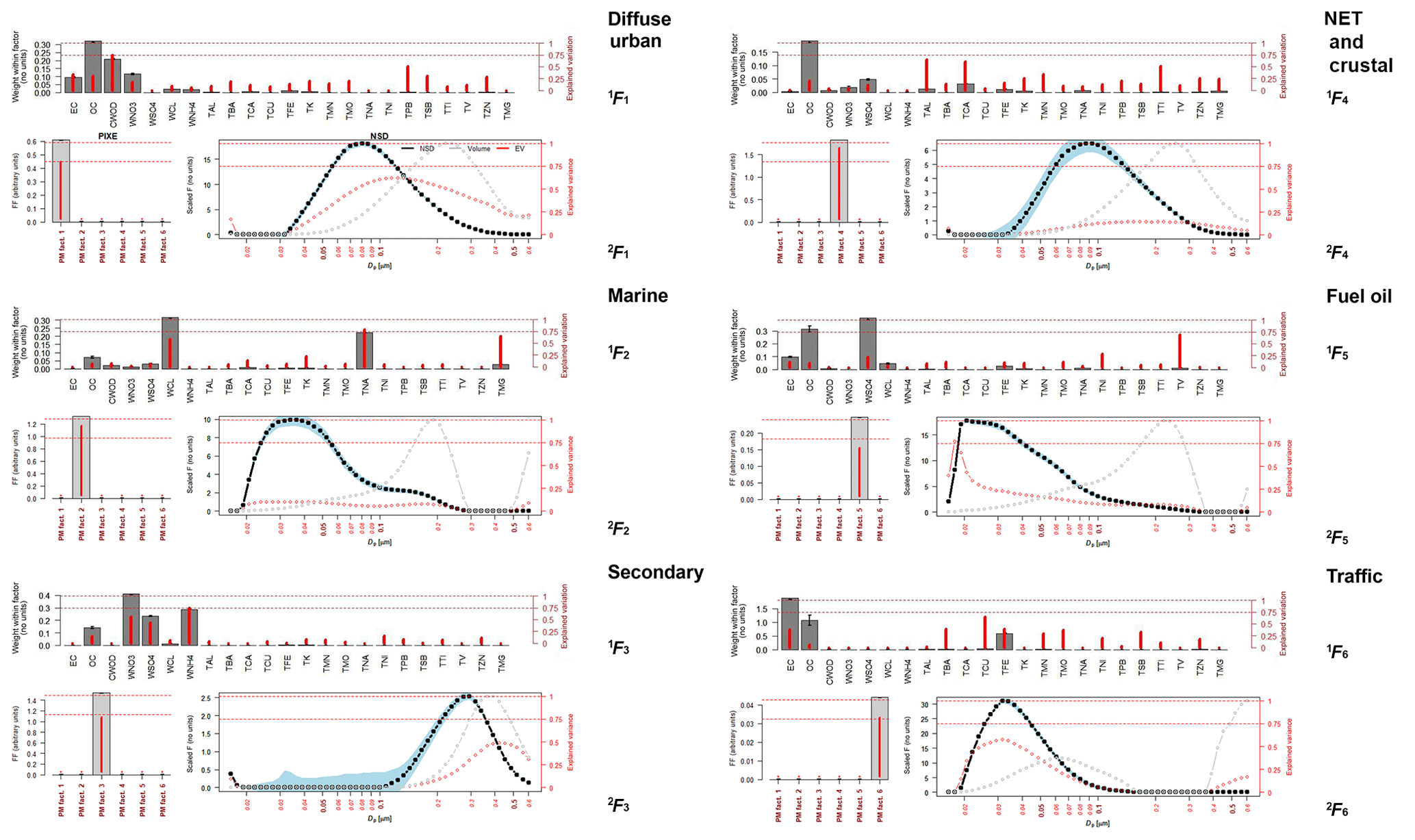
Figure 3 Source profiles ¹F and ²F from both the first and second PMF step using six factors. (Grey bars and black line indicate the values of F; red lines and dots indicate the explained variations; and the grey dotted line indicates the dV/dlogDp values.)

The time series ¹G_k and uncertainties ¹ΔGk from the first PMF analysis of PM₁₀ data were carried over into the second step, where they are combined with the NSD data for PMF analysis (Fig. 2). The uncertainties of the NSD data are taken as an optimized multiple of the NSD values themselves (∼5 % uncertainty, yielding a Q value of 30 333 in the robust mode; see Table S2 for PMF settings). Also in order to encourage ²G_k to be proportional to ¹G_k for k=1–6 (see Table S4), the FKEY matrix is applied to pull elements in the source matrix to zero, as described in Sect. 2.2.6. This ensured that the PMF analysis of the NSD data was driven by the ¹G time series and resulted in a six-factor output in which there were unique contributions from the kth factor ¹G_k from the first analysis to the kth factor ²F_k in the second analysis. This is mainly due to the aggressive pulling of the factor element in ²F applied using FKEY.

When inspecting Fig. 3 it is notable that the source profiles are surprisingly similar to those calculated for the NSD-only and PM₁₀–NSD data in Beddows et al. (2015). The diffuse urban factor has a modal diameter just below 0.1 µm, which is comparable to the same factor in the NSD-only analysis. The marine factor is comparable to the aged marine factor derived from the PM₁₀–NSD analysis. The secondary factor is again the factor with the largest modal diameter (between 0.4 and 0.5 µm), and traffic has as expected a modal diameter between 30 and 40 nm. The fuel oil factor appears to be a combination of a nucleation factor and a mode comparable to diesel exhaust seen in the traffic factor.

3.2 Two-step PMF–LR analysis

Figure S2 shows the results of the linear regression of the NSD data and the PM₁₀ ¹G_k scores, and again what is remarkable is the similarity between these regression source profiles and both the factors derived in Beddows et al. (2015) and those from the two-step PMF–PMF analysis.

This PMF–LR analysis was carried out using daily averaged data, and to obtain hourly information – and thus obtain the diurnal patterns (Fig. S2) – the resulting regression source profiles were refitted to the original NSD data. On inspection of these source profiles and diurnal plots, the negative values make interpretation a struggle, reinforcing one of the four conditions (Hopke, 1991) in the analysis if it is to make sense. We can however fit non-negative gradients using non-negative regression. However, the surprising consequence of applying this constraint is that the same profiles are derived, but they are clipped so that all negative values are replaced by zero values – hence, information is lost. One interpretation of the negative values is that these are particle sinks, but this contradicts the PMF–PMF findings, and hence it is concluded that the PMF–LR analysis only serves as an indication of how the PM₁₀ factors are augmented by the NSD data. If all profiles are shifted to above the zero line, then comparisons to the PMF–PMF data can be made. However, what is interesting to note in this result is the intercept NSD, which is comparable in profile and diurnal pattern to the nucleation mode identified in Beddows et al. (2015). This is a seventh regression source profile, in addition to the six PM₁₀ factors and suggests that although the PMF analysis of the PM₁₀ data alone misses a nucleation factor, this can be recovered in a second analysis as a remainder or bias in the data. Furthermore, this result indicates that the composition of the nucleation NSD factor has no link to the chemical PM₁₀ composition and cannot be used to infer a composition. This is unsurprising given the very small mass contributed by the nucleation-mode particles.

Returning to the PMF–PMF analysis and extending the analysis from six factors to seven factors, an extra row in the FKEY matrix was added to pull all of the ¹G₇ contributions to ²F₇ to zero in the solution (Fig. S1). The same FKEY matrix of fkey₁ and 0 values was used, but this time it was augmented with a seventh row of fkey₂ and zero values. In this case, the fkey₂ values were set to a value of 20.

The same six-factor solution is obtained with the additional seventh factor (Figs. 4 and S3), and, as expected, this seventh factor was a nucleation factor. It was suspected that in the six-factor solution, the nucleation factor was combined with the fuel oil factor. This does not suggest any link between the nucleation and fuel oil factor other than that there was an insufficient number of factors within the model for the two to factorize out of the data, giving the fuel oil NSD profile a more reasonable modal peak between 50 and 60 nm rather than 20, 30 and 60 nm.

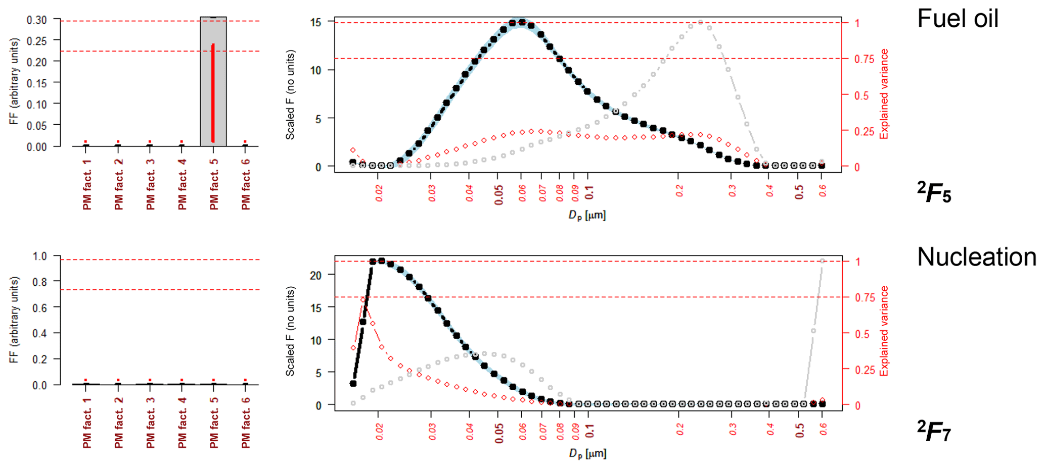
Figure 4 Nucleation and fuel oil factors derived when extending the second PMF analysis from the six factors (shown in Fig. 3) to seven factors. Source profiles ²F₁ to ²F₆ are given in Fig. S3. Each plot shows the output ²F_k. (Grey bars and black line indicate the values of F; red lines and dots indicate the explained variations; and the grey dotted line indicates the dV/dlogDp values.)

Beddows et al. (2015) applied a one-step analysis to three different datasets: PM₁₀-only; NSD-only and PM₁₀–NSD. The analyses of the PM₁₀-only and NSD-only – both with homogeneous units – produced quantitative time series G. This was unlike the analysis of the PM₁₀–NSD with heterogeneous units, which could not apportion its five factors using G but was able to factorize out a nucleation factor from the data, seen also in the four sources in the PMF solution for the NSD-only data. A PM₁₀-only seven-factor solution did not reveal this factor, presumably because the mass associated with nucleation-mode particles is too small to affect composition significantly. Furthermore, fuel oil was not factorized out of the PM₁₀–NSD data and was more likely divided across all five factors.

Another interesting observation is that although only four factors were derived from the PMF analysis of NSD-alone (diffuse urban; secondary; traffic and nucleation), when extra information is included from the PMF analysis of the PM₁₀ data, more information can be extracted from the PMF analysis of the NSD data in the form of the marine, fuel oil and NET and crustal factors. The nucleation factor is only revealed when performing a regression between the NSD size bins and the G scores of the PM₁₀ PMF analysis, which leads to increasing the factor number from six to seven and in turn yields the nucleation profile. It is also reassuring that the bivariate plots for the seven factors (discussed in the next section) correspond to the bivariate plots given in Beddows et al. (2015). Also note that there is no reason why any further investigation might not explore this using more than seven factors. In fact the nucleation factor appears at first sight to be multimodal. However, we restricted our analysis to seven factors, considering it complete in terms of identifying the sources obtained by Beddows et al. (2015).

3.3 Diurnal and bivariate plots

The original PMF was carried out on daily PM₁₀ data, and in order to make diurnal and bivariate plots, a higher time resolution is desirable. It is assumed that the factors derived in the hourly NSD data are the same as those derived from the daily averaged data; i.e. the factors are conserved when averaging the data from hourly to daily data before PMF analysis. Then the hourly NSD data can be fit with the PMF profiles derived from the daily data (see Sect. 2.4). Figure 5 shows the resulting diurnal profiles. The diurnal trends of the parameter c_k (Eq. 6), required to fit the seven daily NSD factors to the hourly NSD data, are shown. These have been scaled to PN (measured in cm⁻³) using the integral of the NSD (Eq. 7). The nucleation factor diurnal trend behaves as expected, rising to a maximum during the day and then falling back down to a minimum at night. This corresponds to the intensity of the sun during the day and the increased likelihood of nucleation on clean days when there is sufficient precursor material to form particles with a low particle condensation sink. The marine factor is also high during the day, presumably due to higher wind speeds. Diffuse urban, NET and crustal and traffic factors all follow a trend which is synchronized to the daily cycle of anthropogenic activity and traffic as influenced by greater atmospheric stability at night. The secondary factor shows a small diurnal range. Fuel oil is highest during the evening and night and may correspond to home heating rather than shipping emissions. The particle size distributions associated with the marine and NET and crustal sources are of limited value as these sources are dominated by coarse particles, beyond the range of the SMPS data, although there is a sharp increase in the volume of the particles above 0.5 µm in the marine factor. As pointed out in Beddows et al. (2015), the marine factor is identified by its chemical profile of sodium and chloride and is accompanied by an aged nucleation mode at around 30 nm. This can be either viewed simply as clean marine air being “polluted” by traffic emission and/or as the consequence of nucleation occurring over at city in clean maritime air masses (Brines et al., 2015). The key point here is that the factors derived in this work are comparable to those factorized in Beddows et al. (2015) using the combined dataset, and the advantage of the two-step approach is that now we have quantified hourly time series G.

Figure 5 Diurnal cycles of the derived PN_k calculated by the fitting of the daily PMF factor profiles to the hourly NSD data fitted (see Eq. 7 and Sect. 2.4). (Left-left column – diurnal trends of PN_k; left-middle column – bivariate plot of PN_k; middle-right – annular plot PN_k; right-right – bivariate plot of PN_k, plotted using the Openair program. Polar plots show a point coloured according to the key, the number concentration at that point on the plot whose distance from the origin represents wind speed and angle wind direction. Likewise for the angular plots, the number concentration is shown for a wind direction at an hour of the day between 00:00 and 23:00.) Note that the diurnal plots do not start at zero.

The hourly contributions are aggregated into daily values and plotted as bivariate plots in Fig. 5 to assist comparison with the daily plots in Beddows et al. (2015). In that work, the same PMF analysis of the NSD data yielded four factors which are named identically to those in the bivariate plots. The similarity of both of the polar and annular plots for each of the six factors supports our previous factor identification. The secondary and diffuse urban factors are background sources with strongest contributions in the evening and morning. Traffic is strongest for all wind speeds from the east, which makes sense since North Kensington is to the west of the city centre of London where traffic is expected to be most dense. Nucleation is also seen to be strongest for wind from the west, which is expected to be cleaner and have a lower condensation sink. NET and crustal and fuel oil factors are similar to the diffuse urban factor, suggesting a similar predominant source location in the centre of London. The marine factor is observed to be strongest for elevated wind speeds for all wind directions, which is consistent with the expected strong contribution for all high wind speeds from the south-west, as observed in the daily polar plots in Beddows et al. (2015).

3.4 Composition associated with the nucleation factor

The nucleation factor was extracted from the two-step PMF–PMF analysis, which included pulling the ¹G₁–¹G₆ values to zero of factor ²F₇. It might be reasonable to suggest that if the two-step PMF–PMF analysis is repeated and the order of analysis of PM₁₀ and NSD datasets reversed that it would be possible to derive the chemical conditions within the atmosphere which were conducive to nucleation. For this, the time series of the four NSD factors (¹G₁–¹G₄) reported in Beddows et al. (2015) were combined with the PM₁₀ data. We again assume that the first PMF step has been carried out and that we are satisfied with how the final solution represents the urban environment of the receptor site and that there are no rotational ambiguities. We then carry out the second step PMF analysis on the 34×591 input matrix ([¹G₁…¹G₄], PM₁₀[PM, PM_carbon, PM_ions, PM_metals]). The hourly output uncertainties from the first PMF analysis of the NSD data ¹ΔG₁…¹ΔG₄ were carried forward into the second PMF analysis by adding them in quadrature to give daily uncertainties. As with the analysis of the auxiliary data in the PM₁₀–NSD data, the measurement uncertainties for the PM₁₀ data (this time the auxiliary data) were naively taken to be 4 times the PM₁₀ matrix. Extra care could have been taken in assigning the PM₁₀ uncertainties, but since we force the output using FKEY, a simpler approach was taken. In fact, the FKEY consisted of a 4×4 diagonal matrix of zero values, with an fkey₁ of 20 for all the off-diagonal positions joined to a 4×30 matrix of zeros. Furthermore, the uncertainty values of the PM₁₀ were scaled until $Q/Q_{\text{theory}}=\mathrm{0.99}$ using parameter b_scale=0.35 (see Table S3 for more details).

Ideally, the chemical data would be limited to the composition of the particles in the same size range as the SMPS data. However, since we are using the PM₁₀ composition data, we can at best describe the composition of the aerosol which accompanied each factor (Fig. S4). For the NSD secondary factor, with its strongest contribution (indicated by the explained variation) ∼400 nm, we have a strong contribution to PM₁₀ and PM_2.5 together with nitrate, sulfate and ammonium. The diffuse urban factor, with its strongest contribution at 100 nm, is accompanied by contributions from elemental carbon and wood smoke, indicative of traffic and recreational wood burning. There are also contributions from barium, chromium, iron, molybdenum, antimony and vanadium, all indicative of non-exhaust traffic emissions and the burning of fuel oil. Similarly, the traffic factor has a modal diameter of roughly 30 nm, which is indicative of exhaust emissions, and this is accompanied by contributions to aluminium, barium, calcium, copper, iron, manganese, titanium and various other metals attributed to vehicles, albeit from tyre or brake wear or resuspension.

The nucleation factor, with its peak ∼20 nm, was associated with marine air, as indicated by the strong contributions to Na, Cl and Mg (Fig. S4). There are also traces of V, Cr and Ni and a high contribution to PM₁₀ mass, which are all associated with marine air. This is explained by an association with the south-westerly wind sector, which brings strong winds and marine aerosol rather than reflecting the composition of the nucleation particles themselves. Marine air is considered to provide the conditions required of an air mass conducive to nucleation, i.e. cleaner air with particles with a low condensation sink. As these air masses pass over the land and eventually into London, anthropogenic precursor gases are added to this air, which then nucleate particles seen at the receptor site as a nucleation mode. This also goes some way to explain the earlier observation of aged nucleation particles observed in the marine factor in Fig. S3. There are also strong contributions to vanadium, which is most likely from an unresolved fuel oil source being mixed into the marine and diffuse urban factors.

4 Conclusions

A two-step PMF analysis method is presented, whereby existing PMF profiles can be extended to incorporate auxiliary data concurrently measured and with different units. This is exemplified using PM₁₀ and NSD data.

When analysing PM₁₀ composition data, the inclusion of auxiliary data such as meteorological, gas and particle number data has proved to give a clearer separation of factors. However, for a successful output, there must be no rotational ambiguity in either the PM₁₀ data or in the auxiliary data. In the ideal case, the individually computed factors G(X), G(Z) and G(X,Z) need to be similar if the joint model is to be successful and not produce large residuals and hence too large a Q value. In the best case, the total weight of the PM₁₀ data can be set higher than the auxiliary data so that the PM₁₀ data drive the analysis. In this work, we present an alternative method called the two-step PMF method. In the first step the PM₁₀ data are PMF-analysed using the standard approach without the inclusion of additional data. An appropriate solution is derived using the methods described in the literature in order to give an initial separation of source factors. The time series G (and errors) of the PM₁₀ solution are then taken forward into the second step, where they are combined with the NSD data. The PMF analysis is then repeated using the combined and mixed unit G time series and NSD dataset. In order to ensure that unique factors are obtained for the G scores, FKEY is used to pull off-diagonal values to zero, thus driving the NSD data. This ensures that the NSD factors are specific to the PM₁₀ solution and the PM₁₀ analysis is not affected by any rotational ambiguity of the NSD data. For our demonstration using the Beddows et al. (2015) analysis, this results in six PM₁₀ factors whose time series are not only apportioned in mass, but the source profiles are identified for the NSD data. Comparisons of the factor profiles, diurnal trends and bivariate plots to those of Beddows et al. (2015) show that this technique produces one solution linking the two separate solutions for PM₁₀ and NSD datasets together. This generates confidence that the NSD and PM₁₀ factors ascribed to one source are in fact attributable to that same source.

Hence, the process starts with a dataset which produces a solution which is sensitive to mass, but the factors more sensitive to number can be accessed using a second step. Furthermore, by exploring a higher number of factors, NSD factors which are insensitive to PM₁₀ mass can be identified as in the case of the nucleation factor. This information can also be extracted using a linear regression, PMF–LR, whereby the size bins of the NSD data are regressed against the PM₁₀ PMF time series. For this dataset, the nucleation factor profile is identified as an intercept within the fitted model, leading to an increase in the number of PMF factors from six to seven.