Accounting for the vertical distribution of emissions in atmospheric CO₂ simulations

Inverse modeling of anthropogenic and biospheric CO₂ fluxes from ground-based and satellite observations critically depends on the accuracy of atmospheric transport simulations. Previous studies emphasized the impact of errors in simulated winds and vertical mixing in the planetary boundary layer, whereas the potential importance of releasing emissions not only at the surface but distributing them in the vertical was largely neglected. Accounting for elevated emissions may be critical, since more than 50 % of CO₂ in Europe is emitted by large point sources such as power plants and industrial facilities. In this study, we conduct high-resolution atmospheric simulations of CO₂ with the mesoscale Consortium for Small-scale Modeling model extended with a module for the simulation of greenhouse gases (COSMO-GHG) over a domain covering the city of Berlin and several coal-fired power plants in eastern Germany, Poland and Czech Republic. By including separate tracers for anthropogenic CO₂ emitted only at the surface or according to realistic, source-dependent profiles, we find that releasing CO₂ only at the surface overestimates near-surface CO₂ concentrations in the afternoon on average by 14 % in summer and 43 % in winter over the selected model domain. Differences in column-averaged dry air mole XCO₂ fractions are smaller, between 5 % in winter and 8 % in summer, suggesting smaller yet non-negligible sensitivities for inversion modeling studies assimilating satellite rather than surface observations. The results suggest that the traditional approach of emitting CO₂ only at the surface is problematic and that a proper allocation of emissions in the vertical deserves as much attention as an accurate simulation of atmospheric transport.

1 Introduction

Reliably predicting future atmospheric concentrations of CO₂, the most important long-lived greenhouse gas, requires a profound understanding of the global carbon cycle, the contributions from anthropogenic and natural fluxes and their sensitivity to climate change, and political and societal drivers. An important tool for advancing our knowledge of the carbon cycle is the integration of CO₂ observations with atmospheric transport simulations in an inverse modeling framework. Global inverse modeling systems helped to better constrain the terrestrial carbon budget, to allocate the global land sink to different continents and ecosystems, and to assess interannual variability and the sensitivity to climate variations (e.g., Bousquet et al., 2000; Chevallier et al., 2010; Peylin et al., 2013; van der Laan-Luijkx et al., 2017; Rödenbeck et al., 2018). Mesoscale inverse modeling systems assimilating observations from dense, regional in situ networks are increasingly being used to study biospheric fluxes at the regional scale (e.g., Sarrat et al., 2009; Goeckede et al., 2010; Broquet et al., 2011; Meesters et al., 2012).

The Paris Climate Agreement, adopted in 2015 (United Nations Framework Convention on Climate Change, 2016), which requires each signing partner nation to accurately report its greenhouse gas (GHG) emissions and to reduce emissions in the future following its Nationally Determined Contribution, has boosted the interest of the atmospheric science community in quantifying not only natural fluxes but also anthropogenic emissions of CO₂. “Top-down” inverse estimation of anthropogenic emissions from atmospheric observations has in fact been proposed as an independent method to complement the traditional “bottom-up” collection of national emission inventories (Nisbet and Weiss, 2010). Several initiatives at the national and international level, such as the World Meteorological Organization (WMO)'s Integrated Global Greenhouse Gas Information System (IG3IS), have been launched to advance and harmonize inverse methods with the long-term vision to establish these methods as a policy-relevant verification and support tool. A summary of the state of the science in inverse modeling for verification of greenhouse gas inventories has recently been presented by Bergamaschi et al. (2018a).

Because of the great challenge of accurately estimating CO₂ fluxes and distinguishing between the biospheric and anthropogenic contributions, the scientific community is calling for a globally integrated carbon observation and analysis system. This system should build on a substantially expanded ground-based and satellite observation capacity and should integrate observations and bottom-up data with atmospheric transport modeling in an inverse framework (Ciais et al., 2014). The individual components and necessary steps towards an operational European system for quantifying anthropogenic CO₂ emissions were outlined in two recent reports to the European Commission (Ciais et al., 2015; Pinty et al., 2017).

A central component of this system is a constellation of CO₂ satellites with imaging capability similar to the CarbonSat concept proposed by Bovensmann et al. (2010). The satellites are currently planned to be implemented in the framework of the European Earth observation Copernicus program and are commonly referred to as Sentinel-CO₂. These satellites should be able to quantify the CO₂ emissions from large sources such as power plants and cities during single overpasses. Corresponding observing system simulation experiments (OSSEs) were presented by Pillai et al. (2016) and Broquet et al. (2018).

In order to establish the requirements for the constellation of Sentinel-CO₂ satellites, the European Space Agency (ESA) has launched several scientific support studies including the use of satellite measurements of auxiliary reactive trace gases for fossil fuel carbon dioxide emission estimation (SMARTCARB), a project that focused on the potential of complementary satellite measurements of NO₂ or CO to improve the quantification of CO₂ emissions from cities and power plants. The present study makes use of the high-resolution atmospheric transport simulations conducted in SMARTCARB to address a specific topic beyond the main focus of the project. The core results of the SMARTCARB study will be presented elsewhere.

Estimating CO₂ fluxes by inverse modeling requires accurate simulation of observed atmospheric CO₂ concentrations. Systematic model biases are particularly critical as they tend to directly translate into biased flux estimates. Several studies investigated the impact of uncertainties in atmospheric transport on simulated CO₂ concentrations and how they could be accounted for in an inverse modeling framework (e.g., Lin and Gerbig, 2005; Chan et al., 2008; Lauvaux et al., 2009). A particular focus was placed on potential biases introduced by errors in vertical transport in the planetary boundary layer (PBL) (Gerbig et al., 2008; Kretschmer et al., 2012, 2014). Uncertainties associated with bottom-up CO₂ emissions were related to uncertainties in the horizontal gridding (Hogue et al., 2016) or the representation of the temporal variability (Liu et al., 2017).

Uncertainties associated with the vertical placement of emissions, conversely, have been largely ignored so far. In fact, in the vast majority of CO₂ atmospheric transport and inverse modeling studies, CO₂ emissions were released exclusively at the surface (e.g., Sarrat et al., 2009; Lauvaux et al., 2009; Broquet et al., 2011; Ganshin et al., 2012; Meesters et al., 2012; Pillai et al., 2016; Lauvaux et al., 2016; Liu et al., 2017; Graven et al., 2018; Fischer et al., 2018). In Lagrangian models such as the Stochastic Time-Inverted Lagrangian Transport model (STILT) (Lin et al., 2003) or FLEXible PARTicle dispersion model (FLEXPART) (Stohl et al., 2005), which are often used in backward, adjoint mode for inverse modeling, particles are typically sampled over a fixed vertical depth above the surface or relative to the height of planetary boundary layer to derive source sensitivities. Similar to the release of emissions at the surface in Eulerian models, this ignores the potentially different sensitivities to emissions from elevated sources.

These approaches in Eulerian and Lagrangian models are questionable given the fact that a large proportion of CO₂ is released from point sources such as power plants well above the surface. Smoke stacks are in fact designed to minimize the impact on concentrations at the ground. This is particularly important during situations with stable inversions in winter or on clear nights. However, even in well-mixed conditions, an elevated release may lead to a faster dilution and different propagation of the signal due to wind speeds and directions changing with altitude.

In the air quality modeling community, the importance of vertically distributing emissions has been recognized much earlier (e.g., Houyoux et al., 2002) and is now well established, especially for species such as SO₂ that are primarily emitted from power plants and industrial sources (Bieser et al., 2011; Mailler et al., 2013; Karamchandani et al., 2014; Guevara et al., 2014). Accounting for plume rise has also been demonstrated to be critical for biomass burning emissions (Achtemeier et al., 2011). The main goal of this study is to demonstrate that this is also critical for the simulation of atmospheric CO₂ concentrations.

We employ very-high-resolution (1.1 km × 1.1 km) simulations for the year 2015 conducted over a 750 km × 650 km wide domain centered in the city of Berlin, Germany. The simulations included separate tracers representing CO₂ emitted only at the surface and CO₂ emitted according to source-dependent vertical profiles. As the domain covered several large coal-fired power plants, we also investigate the impact of dynamically accounting for plume rise versus applying static vertical emission profiles. We focus on domain-averaged statistics rather than on individual plumes and on near-surface concentrations in the afternoon and total columns at satellite overpass time as typically used in inverse modeling. Conditions with a well-mixed and fully developed boundary layer during daytime are expected to minimize the mismatch between model and observations.

2 Data and methods

2.1 COSMO-GHG model

The Consortium for Small-scale Modeling (COSMO) is a limited-area, non-hydrostatic numerical weather prediction (NWP) model developed by the German weather service together with a consortium of seven European weather services (Baldauf et al., 2011). In addition to operational weather prediction, the model is applied widely for climate and air pollution research in various modified and extended versions (e.g., Rockel et al., 2008; Davin et al., 2011; Vogel et al., 2009; Zubler et al., 2011), making COSMO a versatile community model.

In the project CarboCount-CH (Oney et al., 2015), COSMO was extended with a module for the simulation of greenhouse gases, hereafter referred to as COSMO-GHG. The extension was built on a newly developed tracer module (Roches and Fuhrer, 2012), which replaced the previous non-uniform treatment of meteorological tracers in the model. A similar, independently developed COSMO-based CO₂ model system was presented by Uebel and Bott (2018).

COSMO-GHG was first applied by Liu et al. (2017) to study the spatiotemporal patterns of fossil fuel CO₂ in Europe. They concluded that fossil fuel CO₂ accounts for more than half of the total (anthropogenic plus biospheric) temporal variations in atmospheric CO₂ over large parts of Europe. Furthermore, they evaluated the model against observations, demonstrating that the simulated fossil fuel variations favorably agreed with observations of fossil fuel CO₂ derived from concurrent measurements of CO and ¹⁴CO₂.

COSMO is the first operational NWP model worldwide that is running on hardware accelerated using graphical processing units (GPUs) (Fuhrer et al., 2014). This highly efficient code is operationally used by the Swiss weather service MeteoSwiss and has been applied for decadal convection-resolving climate simulations (Leutwyler et al., 2017). In the framework of SMARTCARB, the modules of the GHG extension were ported to the GPU version following the concept of OpenACC compiler directives, which is a high-level approach to offload compute-intensive parts to a GPU accelerator (Lapillonne and Fuhrer, 2014). Benchmark tests showed that the GPU version achieved a speedup by a factor of 6, which allowed for an increase in spatial and time resolution, and which greatly reduced the computational (and energy) costs of the simulations conducted in this study.

2.2 Model domain and setup

The model simulations were conducted in the framework of the project SMARTCARB, which aimed at studying the potential benefit of adding an NO₂ or CO channel to the instrument package of a future CO₂ satellite mission with respect to quantifying CO₂ emissions from strong localized sources such as cities and power plants. For this purpose, a model domain was selected covering the city of Berlin as well as several large power plants in Germany, Poland and Czech Republic. The domain extended approximately 750 km in the east–west and 650 km in the south–north directions to cover at least a complete 250 km wide satellite swath on either side of the city. Berlin was selected not only because it is one of the largest cities in Europe, but also because it is rather isolated, and because it has already been investigated in previous CO₂ modeling and observation studies (Pillai et al., 2016; Hase et al., 2015). Simulations were conducted for the complete year 2015 at 1.1 km × 1.1 km horizontal resolution and 60 vertical levels with a top at 24 km. The lowest model layer had a thickness of 20 m. The vertical allocation of the emissions relative to this vertical resolution of the model will be described in Sect. 2.4. The high horizontal resolution was selected to comply with the small pixel size of 2 km × 2 km of the planned CO₂ imaging satellite, keeping in mind that the effective resolution of Eulerian transport models is much lower than the spacing of the model grid (Kent et al., 2014).

The simulations included a total of 50 different passively transported tracers of CO₂, CO and NO_x. The tracers represented different sources, release times or release altitudes and included background tracers constrained at the lateral boundaries by global-scale models. Two additional tracers for biospheric fluxes (respiration and photosynthesis) were included for CO₂, and four additional tracers with varying e-folding lifetimes of 2, 4, 12 and 24 h for NO_x. In this study, however, we focus on only a few of these tracers, notably on the following four anthropogenic CO₂ emission tracers:

• CO2_VERT: all anthropogenic emissions in the model domain released according to source-specific vertical profiles.

• CO2_SURF: same as CO2_VERT but all emissions released at the surface, i.e., into the lowest model layer.

• CO2_PP-PR: emissions from the six largest power plants with explicit plume rise calculations.

• CO2_PP-EMEP: emissions from the six largest power plants released according to a fixed vertical emission profile.

The simulations were nested into the operational European COSMO-7 analyses of MeteoSwiss, which provided the lateral boundary conditions for meteorological variables (temperature, pressure, wind, humidity, clouds) at 7 km horizontal and hourly temporal resolution. Because of the relatively small domain, these boundary conditions provided a strong constraint for the meteorology within the domain. For CO₂, lateral boundary conditions were obtained from a global free-running high-resolution CO₂ simulation (T1279, 137 levels, ∼15 km horizontal resolution) provided by the European Centre for Medium-Range Weather Forecasts (ECMWF) through the European Earth observation Copernicus program (Agustí-Panareda et al., 2014). The simulation was indirectly constrained by in situ data by using a global climatology of optimized biospheric fluxes computed with the CO₂ assimilation system of Chevallier et al. (2010).

2.3 Emissions and biospheric fluxes

Anthropogenic emissions were obtained by merging the Netherlands Organisation for Applied Scientific Research European Monitoring Atmospheric Composition and Climate version 3 (TNO/MACC-3) inventory with a detailed inventory available for the city of Berlin. Dedicated municipal inventories can accurately account for the specific conditions and activities in a city and may therefore significantly deviate from inventories obtained by simple downscaling from larger-scale inventories (Timmermans et al., 2013; Gately and Hutyra, 2017).

Version 3 of the TNO/MACC inventory was used, which has an improved representation of point sources as compared to version 2 described in Kuenen et al. (2014). It has a nominal resolution of $\mathrm{1}/{\mathrm{16}}^{\circ }\times \mathrm{1}/{\mathrm{8}}^{\circ }$ (approximately 7 km × 7 km) but additionally reports the emissions from strong point sources at their exact location. Emissions are provided separately for different source categories following the Standardized Nomenclature for Air Pollutants (SNAP) classification (European Environment Agency, 2002). The emissions of the year 2011 were taken, which was the most recent year available from the inventory.

The city of Berlin has developed a very detailed inventory for about 30 air pollutants and greenhouse gases for seven major source categories. The inventory was provided in a Geographic Information System (GIS) format as a collection of shape files representing individual area, point and line sources. The latest available year was 2012. In our simulations, separate tracers were included for three broad source groups: traffic, industry and heating. The attribution of the 10 SNAP categories in TNO/MACC-3 and the seven source categories in the Berlin inventory to these groups are described in detail in the final report of the SMARTCARB project (Kuhlmann et al., 2019).

Both inventories were projected onto the COSMO model grid (rotated latitude–longitude grid with the North Pole at 43^∘ N and 10^∘ W, ${\mathrm{0.01}}^{\circ }\times {\mathrm{0.01}}^{\circ }$ resolution) using mass-conservative methods. Point sources were placed into the proper COSMO grid cell. As a last step, the two inventories were merged using a mask for the city of Berlin. The merged emission e per grid cell was estimated as $e=(\mathrm{1}-f)e_{\mathrm{TNO}}+e_{\mathrm{Berlin}}$, where f is the fraction of the grid cell area covered by Berlin.

Figure 1 presents a map of the CO₂ inventory of Berlin in the original format and after projection onto the COSMO grid. The rasterized map reveals 22 strong CO₂ point sources, which together account for 41 % of the total emissions in the city. The two horizontal stripes correspond to the paths of airplanes taking off and landing at the two main airports.

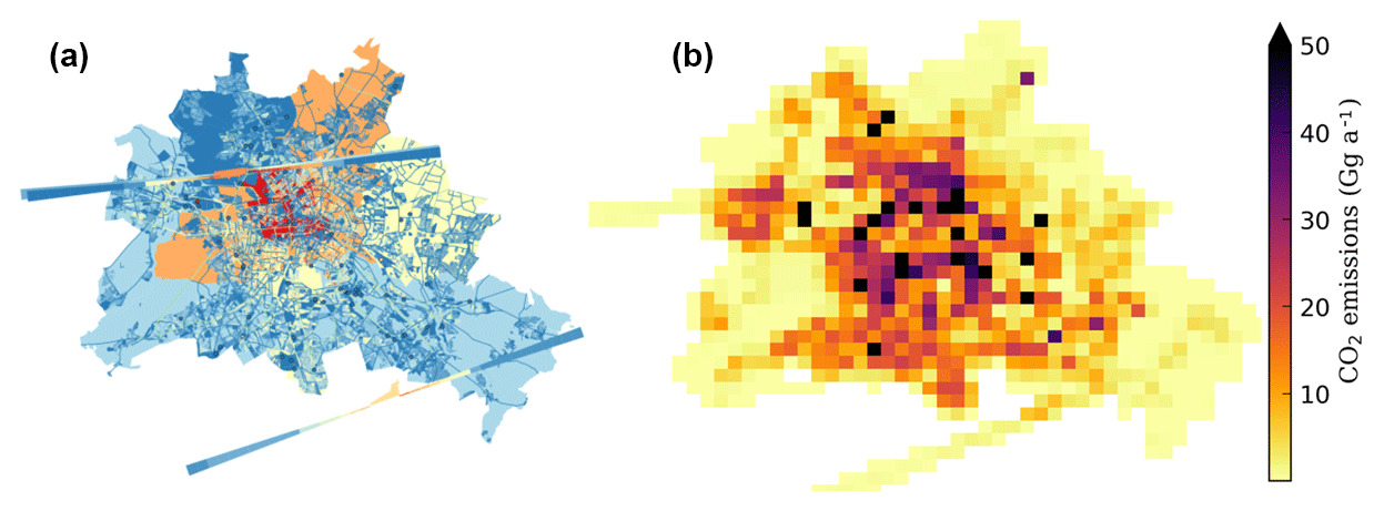
Figure 1 (a) Schematic of CO₂ emissions in the Berlin inventory with point, line and area sources from different emission categories. Point, line and area sources are in different units (in kg s⁻¹ for point, $\mathrm{kg}{\mathrm{s}}^{-\mathrm{1}}{\mathrm{m}}^{-\mathrm{1}}$ for line and $\mathrm{kg}{\mathrm{s}}^{-\mathrm{1}}{\mathrm{m}}^{-\mathrm{2}}$ for area sources) each being colored separately between minimum and maximum values. (b) Total CO₂ emissions re-projected and rasterized onto the COSMO model grid.

In order to calculate hourly emissions as input for the model simulations, temporal scaling factors were applied describing diurnal, day-of-week and seasonal variations. The same temporal profiles were used as in Liu et al. (2017), which are based on factors originally developed for air pollution modeling (Builtjes et al., 2003). These profiles depend on SNAP category and, except for diurnal profiles, on country. Diurnal profiles were matched to the local time of Germany.

Biospheric CO₂ fluxes due to gross photosynthetic production and respiration were computed at the resolution of the COSMO model using the Vegetation Photosynthesis and Respiration (VPRM) model (Mahadevan et al., 2008). This diagnostic model is based on meteorological input (2 m temperature and downward shortwave radiation at the surface) along with the Enhanced Vegetation Index (EVI) and Land Surface Water Index (LSWI) calculated from MODIS satellite reflectances. These indices were available as an 8-day product (MOD09A1, V006) at 500 m spatial resolution. Vegetation classes were determined from the 1 km SYNMAP land cover map (Jung et al., 2006). Model parameter values describing the fluxes from different vegetation types were taken from a previous study (Kountouris et al., 2018), in which they were optimized using data from 47 European eddy covariance measurement sites for the year 2007. The model was run offline for the entire year 2015, driven by the highest resolution ECMWF meteorological data available.

2.4 Vertical allocation of emissions and plume rise

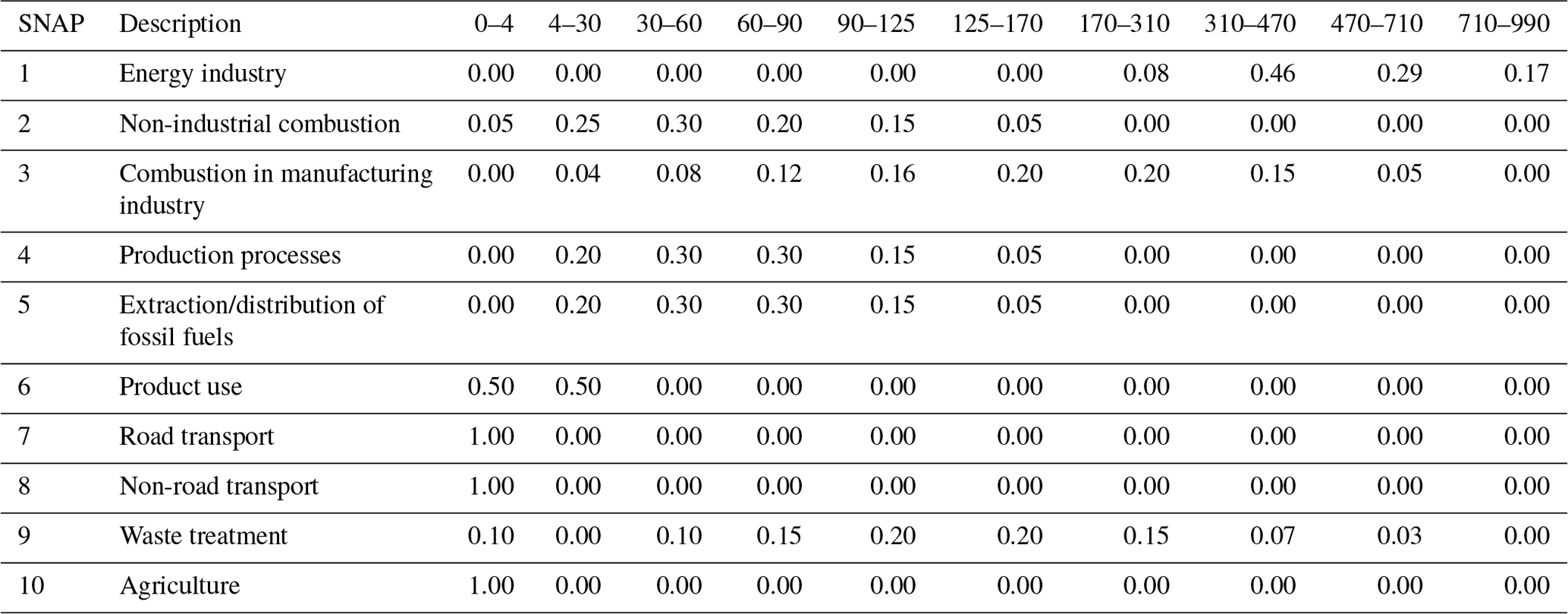
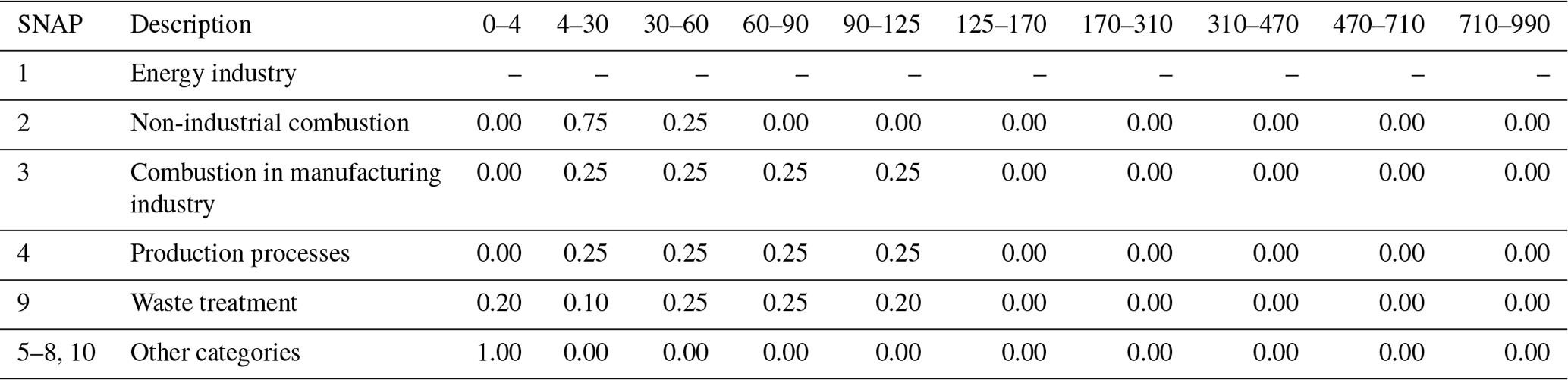
Emissions were distributed in the vertical using source-specific profiles developed for the European Monitoring and Evaluation Program (EMEP) (see, e.g., Bieser et al., 2011). For the purpose of the present study, the number of vertical layers was increased from 7 to 10 to enable a finer allocation to the model layers of COSMO-GHG. Specifically, the layers 4–90 m and 90–170 m of the original EMEP profiles were divided into three and two sublayers, respectively. The attribution of emissions to these sublayers was done in a rough way, for example, by placing a larger proportion of emissions from “combustion in manufacturing industry” into the upper parts but distributing emissions from “non-industrial (residential) combustion” rather evenly over the three layers between 4 and 90 m, considering that industrial sources are likely to emit at higher altitudes. The profile for SNAP 9 (waste) was modified in two ways: (i) by moving 10 % from higher layers to the lowest layer to account for CO₂ emissions from landfills and waste water treatment plants, and (ii) by moving the large fractions originally placed into the layers 170–310 m (40 %) and 310–470 m (35 %) into lower layers between 90 and 310 m. This latter modification was made following the study of Pregger and Friedrich (2009), which showed that the emission-weighted height of waste incinerator stacks in Germany is only about 100 m and that 90 % of the corresponding emissions including plume rise are expected to occur below 300 m.

The modified EMEP profiles are presented in Table 2 and illustrated in Fig. 2a. They were only applied to point sources such as power plants and large industrial facilities. A different set of profiles with lower average emission heights was applied to area sources, as these represent much weaker and more dispersed sources. The corresponding profiles are presented in Table 3 and Fig. 2b. The motivation for this distinction is best illustrated for SNAP category 2, residential and other non-industrial heating. In the case of point sources, these are large heating facilities such as combined heat and power plants with tall stacks. In the case of area sources, in contrast, these are mostly private heating systems releasing CO₂ through chimneys at roof level. This is reflected in our profiles for SNAP 2 area sources being limited to the layers between 4 and 60 m above surface.

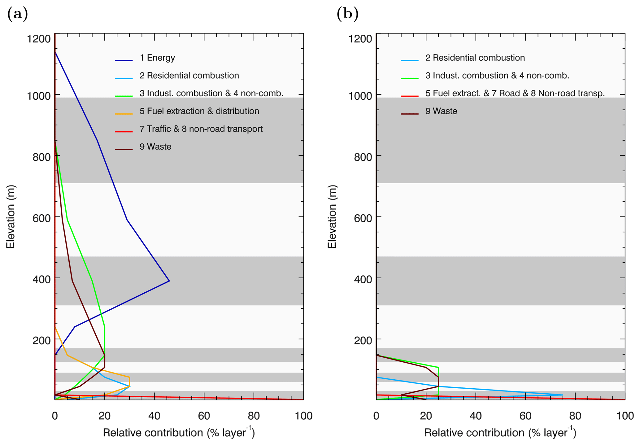
Figure 2 Vertical emission profiles applied for (a) point sources and (b) area/line sources. The alternating gray and white backgrounds denote the vertical layers.

Table 1 Stack parameters used for plume rise calculation for the six largest power plants in the model domain.

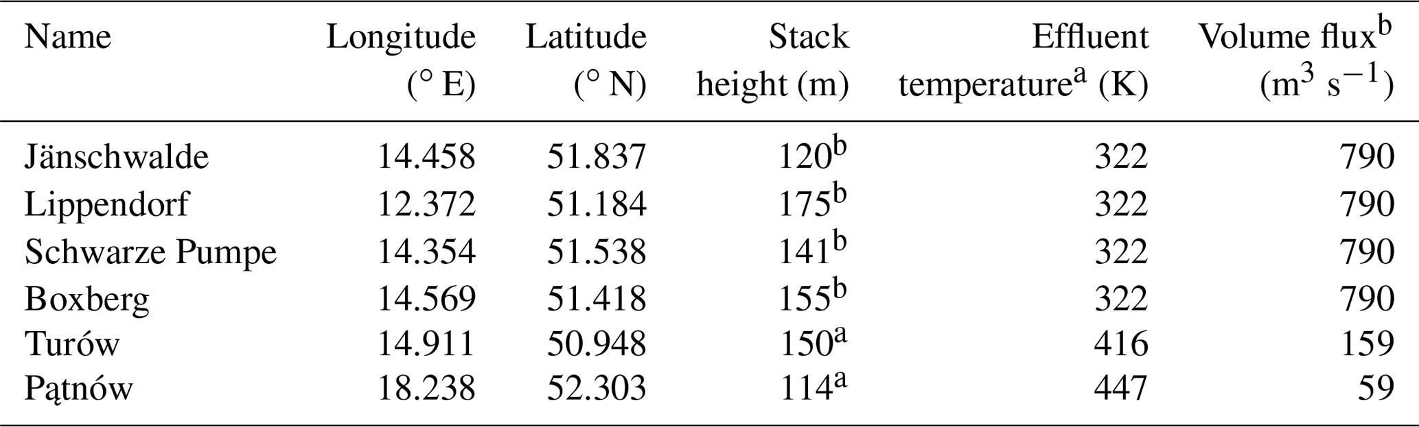
^a Average parameters by fuel and plant capacity taken from Pregger and Friedrich (2009). ^b https://de.wikipedia.org/wiki/K\”{u}hlturm (last access: 28 August 2018).

Table 2 Vertical emission profiles for point sources for different SNAP categories as fractions of the total emitted mass per vertical layer. Layers are denoted by their lower and upper limits (meters above ground).

As noted by Bieser et al. (2011), the EMEP profiles are based on very limited information originally collected for the city of Zagreb, Croatia. They therefore proposed a different set of profiles based on plume rise calculations for a large number of point sources across Europe. Their study indicated that the vertical placement of emissions in the EMEP profiles is too high for combustion processes (SNAP 1, 2, 3 and 9) but too low for production processes (SNAP 4 and 5). For SNAP 1 (power plants), for example, they proposed a median release height of about 300 m, whereas the median in the EMEP profiles is about 400 m.

Although we did not apply the profiles of Bieser et al. (2011), our modification of SNAP 9 and the distinction between point and area sources effectively reduces the emission heights of CO₂ compared to the standard EMEP profiles. Furthermore, for the 22 largest point sources in Berlin as well as the six largest power plants in the model domain in Germany (Jänschwalde, Lippendorf, Boxberg, Schwarze Pumpe) and Poland (Turów, Pątnów), the static EMEP SNAP 1 profiles were replaced by dynamic plume rise simulations for each hour of the year.

The effective emission height can be much higher than the geometric height of a stack because of the momentum and buoyancy of the flue gas. In general, plume rise depends on stack geometry (height and diameter), flue gas properties (temperature, humidity, exit velocity) and meteorological conditions (wind speed, atmospheric stability). Plume rise and the vertical extent of the plumes were calculated using the empirical equations recommended by the Association of German Engineers (VDI – Fachbereich Umweltmeteorologie, 1985), which are based on the original work of Briggs (1984). Hourly profiles of wind and temperature for the year 2015 were extracted from the COSMO-7 analyses of MeteoSwiss at the locations of the individual stacks. For power plants outside Berlin, typical stack and flue gas parameters were mainly taken from published statistics for Germany (Pregger and Friedrich, 2009), since these parameters are not publicly available (see Table 1). For stacks in Berlin, parameters were included in the emission inventory provided by the city of Berlin.

Table 3 Vertical emission profiles for area sources for different SNAP categories as fractions of the total emitted mass per vertical layer. Layers are denoted by their lower and upper limits (meters above ground). Emissions in SNAP 1 are released exclusively from point sources.

Two complicating factors were not considered in the present study. The European standards for large combustion plants (http://data.europa.eu/eli/dec_impl/2017/1442/oj, last access: 26 March 2019) require the flue gas to be cleaned for sulfur and nitrogen oxides. As a consequence of the chemical washing process, the temperature of the flue gas is reduced to a level where it can no longer be released via a classical smoke stack (Busch et al., 2002). In order to avoid reheating, the flue gas is often directed to the cooling tower and mixed into its moist buoyant air stream. This is true for the major German power plants in the domain, whereas the power plants Turów and Pątnów in Poland were, to the best of our knowledge, still equipped with smoke stacks in 2015. Plume rise computations are much more complex in the case of cooling towers due to latent heat release and the interaction with moisture in the ambient air (Schatzmann and Policastro, 1984). The additional release of latent heat may enhance plume rise by 20 % to 100 % compared to a dry plume (Hanna, 1972). Second, large power plants such as Jänschwalde are equipped with multiple cooling towers a short distance from each other. Their plumes tend to interact in a way that enhances plume rise, an effect that additionally depends on the alignment of the towers relative to the flow direction (Bornoff and Mokhtarzadeh-Dehghan, 2001). Neglecting these effects may thus underestimate true plume rise in our calculations.

3 Results

3.1 Plume rise at power plants

An example for the results of the plume rise simulations are presented for Jänschwalde, the largest power plant in the domain. Figure 3a shows the hourly evolution of the plume center heights during the year 2015. Plumes typically rise 100 to 400 m above the top of the cooling tower, but occasionally much further when both winds and atmospheric stability are low. Plume rise varies strongly from day to day and shows a pronounced seasonal cycle. Plumes rise on average to 360 m above ground in summer but only to 250 m in winter. Due to the diurnal evolution of the PBL, plume rise also varies with the hour of the day, except during winter. In summer, the amplitude of this diurnal variability is about 150 m, with a broad minimum at night from 21:00 to 08:00 LT (19:00 to 06:00 UTC) and a peak in the early afternoon.

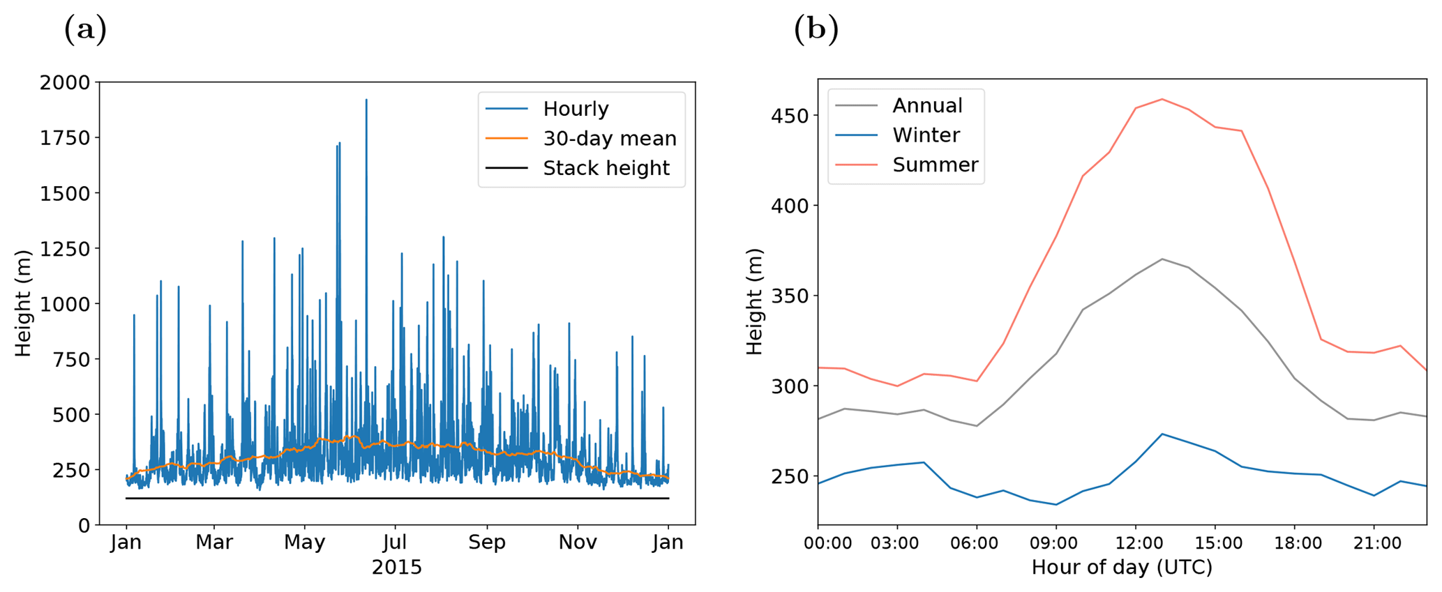
Figure 3 Effective CO₂ emission heights at the power plant in Jänschwalde, Germany, based on plume rise calculations. (a) Hourly plume rise in 2015. The orange line is a 30-day moving average. The black solid line denotes the height of the cooling tower (120 m). (b) Mean annual, winter (DJF) and summer (JJA) diurnal cycles.

Figure 4 compares the histograms of plume rise at Jänschwalde in summer and winter to the standard EMEP SNAP 1 profile of Fig. 2. In agreement with Bieser et al. (2011), the computed profiles tend to place emissions significantly lower compared to EMEP, even in summer. Median and mean effective emission heights in 2015 were 266 and 310 m above ground, respectively. For the smaller power plant (Lippendorf), these numbers were 187 and 210 m. Simulated plume rise for these two power plants was thus at least 100 m lower compared to the EMEP profile. The large fraction of emissions placed above 500 m in the EMEP profile seems particularly unrealistic. Our plume rise calculations are more consistent with the profiles recommended by Bieser et al. (2011).

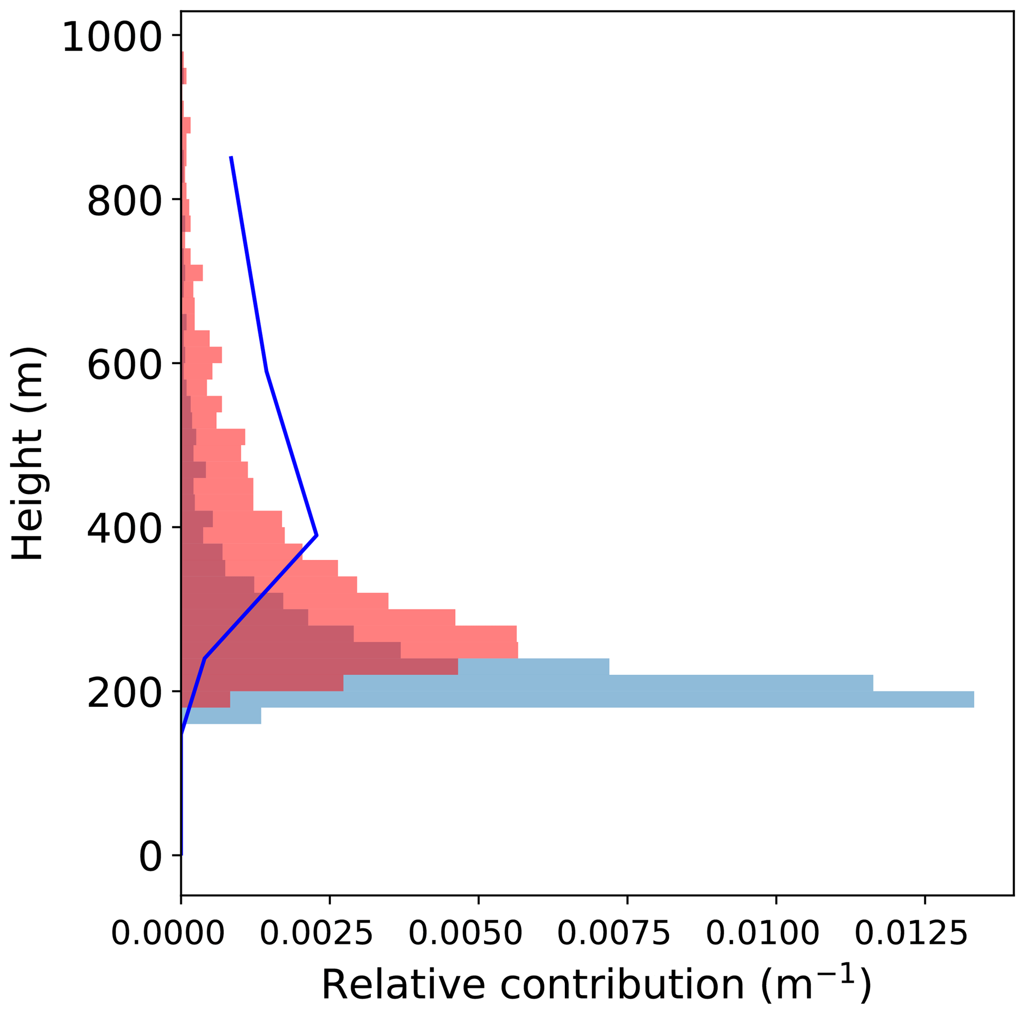
Figure 4 Normalized histogram of plume altitude above ground at the Jänschwalde power plant in winter (blue) and summer (red). The blue line shows the EMEP standard profile for power plants for comparison. Areas below the curves integrated along the vertical axis are normalized to 1.

3.2 Emission profiles over Berlin

The main emission sources of CO₂ in Berlin are “traffic”, “private households and public buildings”, “industry”, “trade and others” and the “transformation sector” which includes large facilities for heat and electricity production. In 2015, traffic only accounted for 29 % of all emissions, households and industry for 27 % (Amt für Statistik Berlin-Brandenburg, 2018). By far the largest single source was the transformation sector with a share of 42 % of the total. As a result, a significant fraction of emissions is released through stacks.

Figure 5 shows the monthly mean vertical profiles of CO₂ emissions from Berlin in a winter month (February) and a summer month (August) as used in our simulations. The profiles reflect the superposition of emissions from different sectors with different vertical profiles (see Fig. 2) and different seasonal contributions. In February, for example, residential heating is an important source between 4 and 60 m above ground, whereas emissions in these layers are almost completely absent in August. Although in both months the profiles have a pronounced peak at the surface, 36 % of CO₂ is released above 90 m in February, with that share rising to 58 % in August when residential heating is low. These numbers suggest that a proper vertical allocation of emissions is important even in cities.

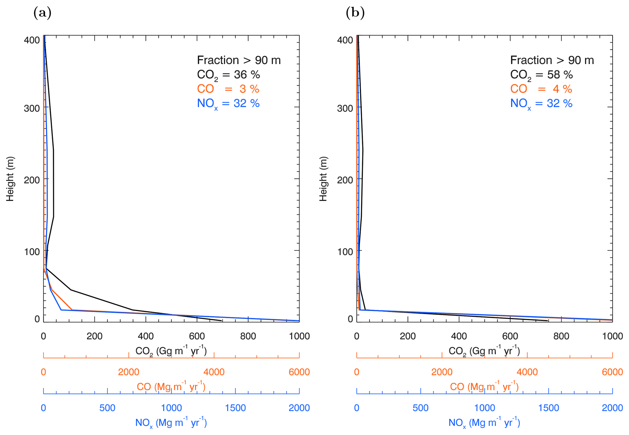
Figure 5 Monthly mean vertical emission profiles of CO₂, CO and NO_x over Berlin in (a) February and (b) August.

The vertical profiles of the emissions of CO and NO_x are overlaid in Fig. 5 for comparison, since coincident measurements of NO₂ or CO may be used by a future CO₂ satellite for emission quantification. Both CO and NO_x have a more pronounced peak at the surface due to the larger proportion of traffic emissions. Similar to CO₂, a large (albeit smaller) fraction of NO_x is emitted well above ground by large point sources. Interestingly, these sources emit very little CO, suggesting efficient combustion or cleaning of the exhaust. The fraction of CO released above 90 m is below 5 %, in sharp contrast to CO₂.

3.3 CO₂ at the surface

Maps of the monthly mean afternoon CO₂ dry air mole fractions (hereafter referred to as “concentrations”) in the lowest model layer (0–20 m) from all anthropogenic emissions within the model domain are presented in Fig. 6 for January and July, respectively. Afternoon values were selected since current inversion systems usually assimilate only observations in the afternoon when vertical concentration gradients are smallest (e.g., Peters et al., 2010). Figure 6a and c show the results for the tracer CO2_VERT, with vertically distributed emissions, while Fig. 6b and d show the tracer CO2_SURF, with all emissions concentrated at the surface. For all power plants labeled in the figure, plume rise was explicitly simulated for the tracer CO2_VERT.

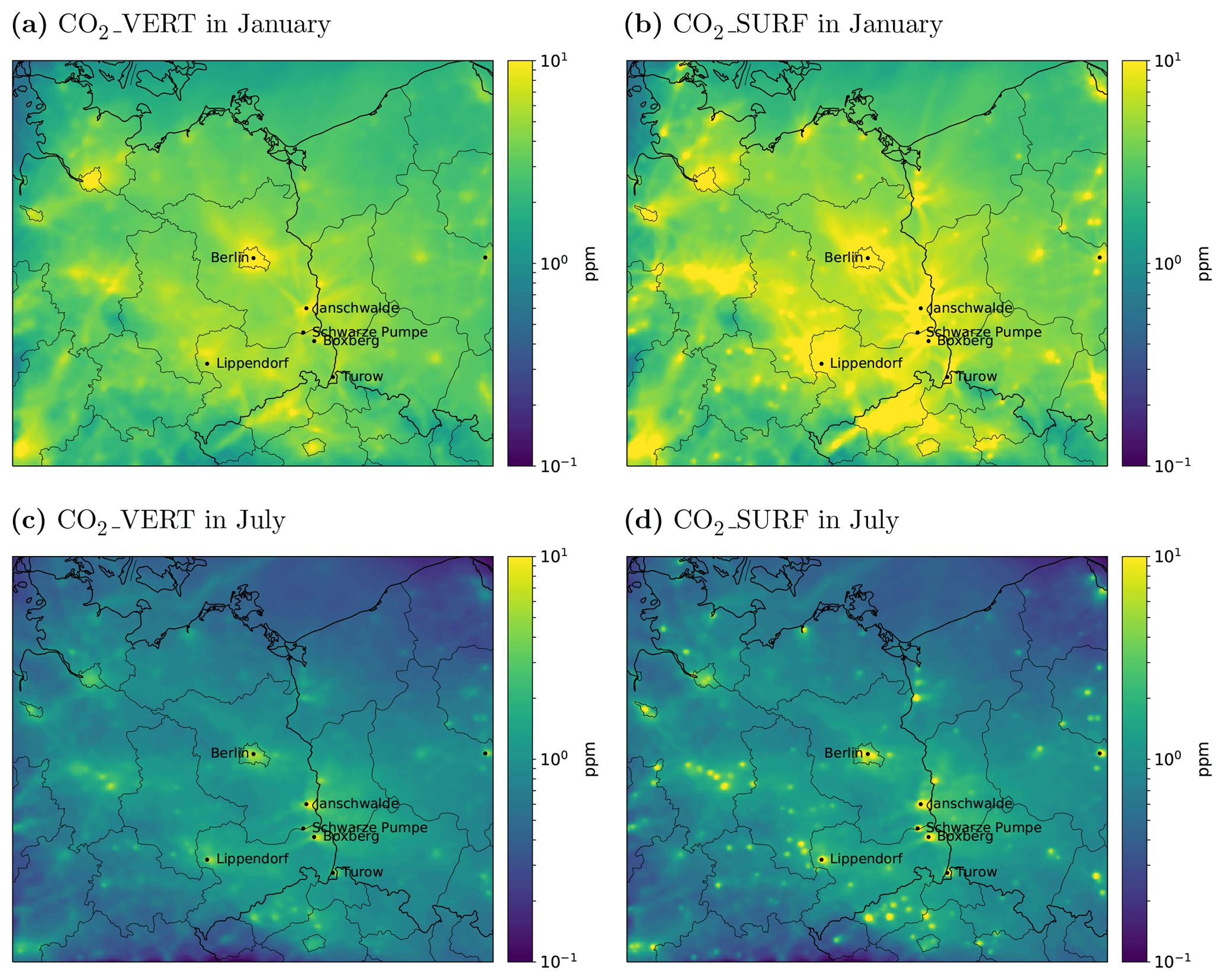
Figure 6 Mean afternoon (14:00–16:00 LT) near-surface CO₂ in (a, b) January and (c, d) July contributed by all anthropogenic sources in the domain. (a, c) Tracer CO2_VERT released according to realistic vertical profiles. (b, d) Tracer CO2_SURF released only at the surface.

The concentrations are generally higher in January than in July due to higher emissions and reduced vertical mixing in winter. The concentrations are also significantly higher when all CO₂ is released at the surface. The main reason for these differences are power plants and other point sources, which stand out prominently in the maps for the tracer CO2_SURF but not for CO2_VERT.

As shown in Fig. 7, the differences are much larger in winter than in summer. In summer, power plant emissions are mixed efficiently over the depth of the afternoon PBL. Since this mixing is not instantaneous, differences are noticeable close to the sources but fade out rapidly with increasing distance. In winter, conversely, when vertical mixing is weak, the differences between the two tracers remain well above 1 ppm over distances of a few tens of kilometers downstream, occasionally over 100 km or more.

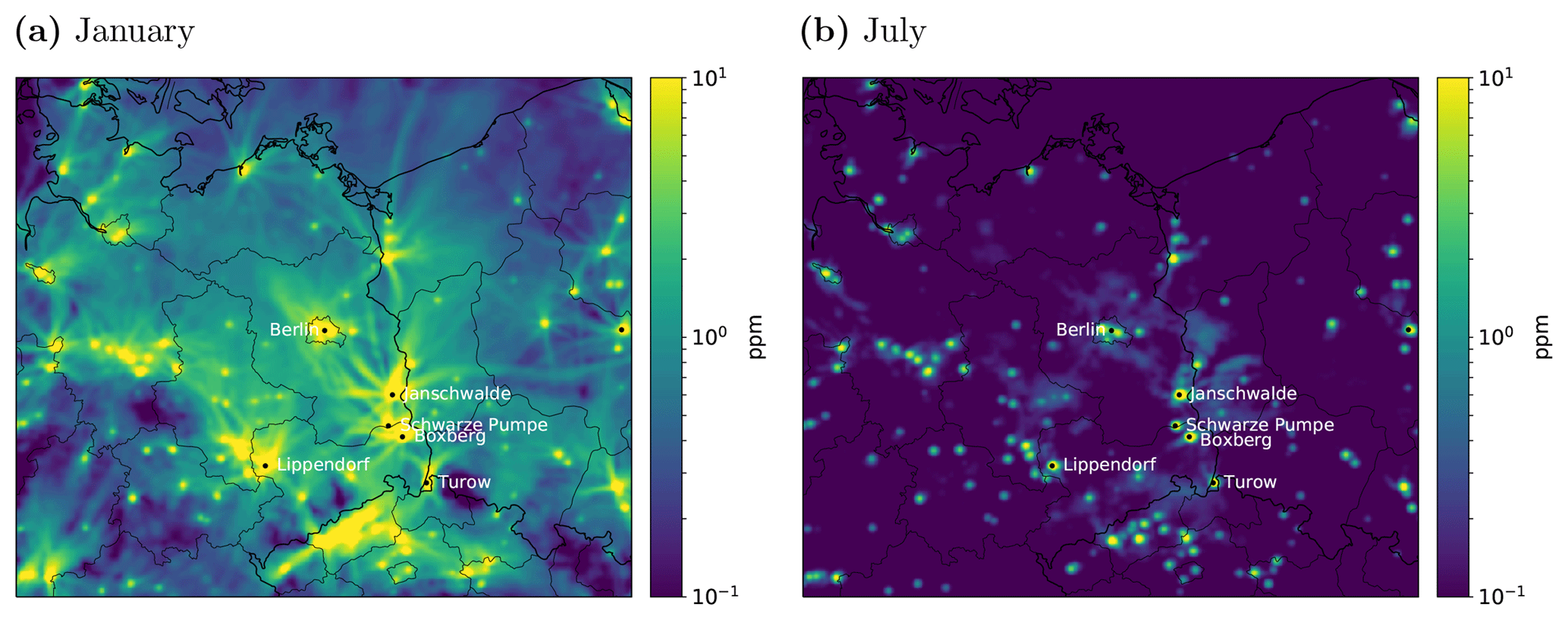
Figure 7 Difference in mean afternoon (14:00–16:00 LT) near-surface CO₂ between tracers CO2_SURF and CO2_VERT in (a) January and (b) July.

Domain-averaged monthly mean diurnal cycles of the two tracers are presented in Fig. 8 for the months of January and July. Consistent with the maps, the concentrations of CO2_SURF are significantly higher than those of CO2_VERT. This difference is around 1.6 ppm in January and almost constant during the day. The variations during the day appear to be dominated by the diurnal cycle of the emissions rather than by the dynamics of the PBL.

Figure 8 Mean diurnal cycles of the tracers CO2_VERT and CO2_SURF in January and July.

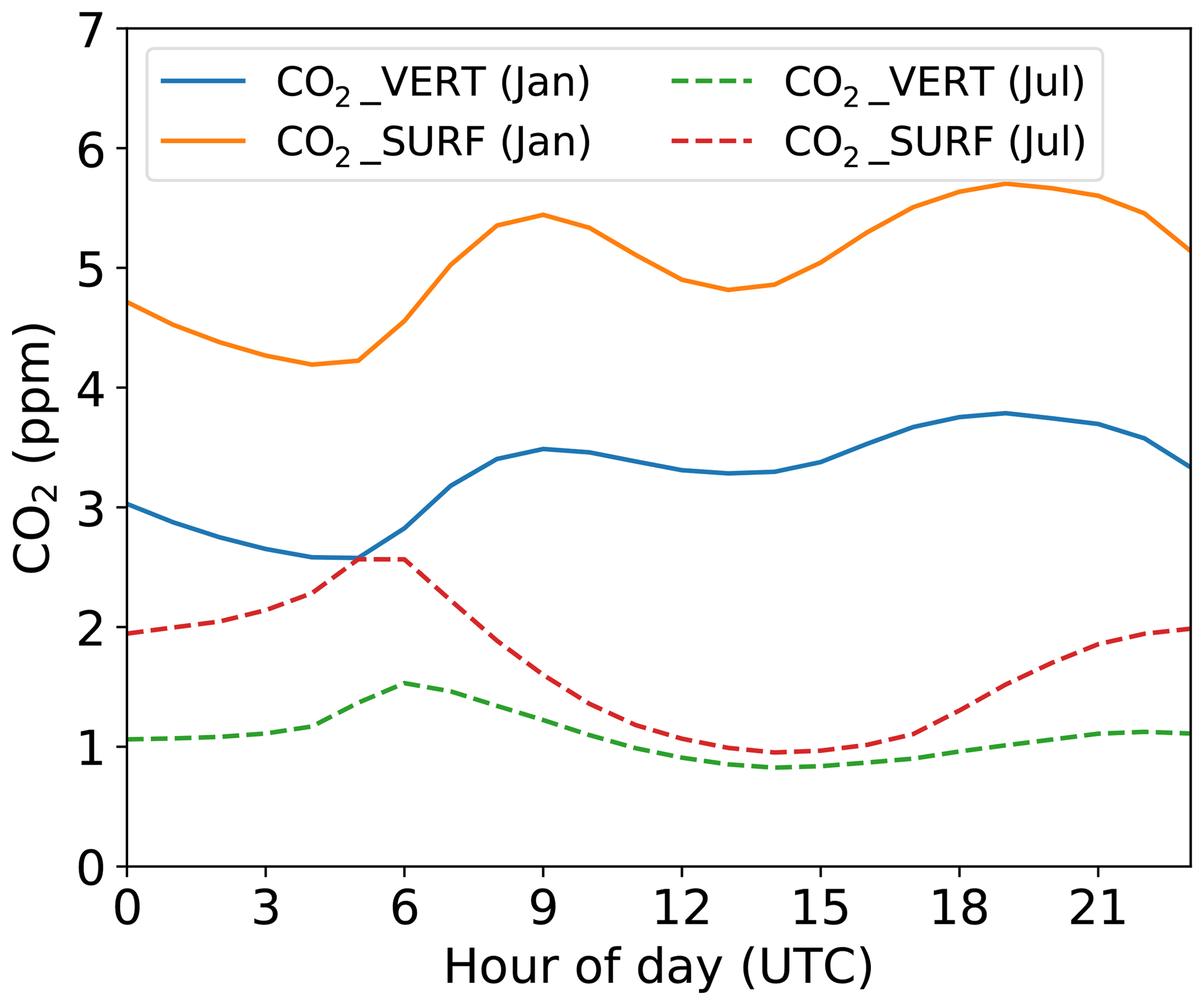
In summer, the differences are generally smaller and exhibit a pronounced diurnal cycle. Differences are about 1 ppm at night and almost vanish (about 0.1 ppm) in the afternoon. Due to the low PBL at night, the concentrations increase overnight despite relatively low emissions. This increase is much more pronounced for tracer CO2_SURF, which is susceptible to surface emissions from point sources that do not stop at night. The tracer CO2_VERT only shows a marked increase during the early morning hours when traffic increases and the PBL is still low. Emissions from point sources, on the other hand, are likely released above the nocturnal PBL, leading to marked differences between CO2_VERT and CO2_SURF at night.

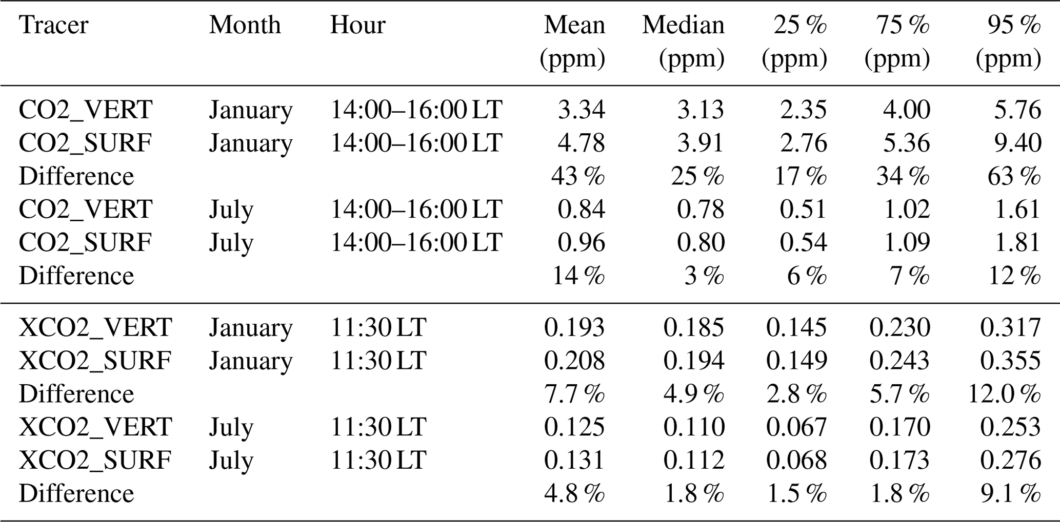
Statistics of the afternoon concentrations of the two CO₂ tracers are summarized in Table 4 in terms of mean values and different percentiles of the frequency distribution. Domain-averaged CO₂ concentrations are 43 % higher in January when all CO₂ is released at the surface compared to when emissions are distributed vertically. The differences are larger for the high percentiles, suggesting that background values are less affected than peak values. This is understandable as vertical mixing tends to reduce the differences with increasing distance from the sources. In summer, the differences are generally much smaller, but as suggested in Fig. 8, this is only true for afternoon concentrations. Mean differences in the afternoon are of the order of 14 %. Again, higher percentiles tend to show larger differences. The impact on observations from tall tower networks measuring CO₂ some 100 to 300 m above the surface (Bakwin et al., 1995; Andrews et al., 2014) will likely be somewhat smaller than suggested by the numbers above, especially in winter when the atmosphere is less well mixed.

3.4 Column-averaged dry air mole XCO₂ fractions

As shown in the previous section, the choice of vertical allocation of the emissions has a large impact on ground-level concentrations. Since the tracers CO2_VERT and CO2_SURF are based on the same mass of CO₂ emitted into the atmosphere and only differ by the vertical placement of this mass, differences in column-averaged dry air mole fractions (ratio of moles of CO₂ to moles of dry air in the vertical column, XCO₂) are expected to be small. However, since wind speeds tend to increase with altitude, CO₂ emitted at higher levels is more likely to be transported away from the sources and leave the model domain more rapidly.

Figure 9 Column-averaged dry air mole fractions (XCO₂) at 11:30 LT in (a, b) January and (c, d) July contributed by all anthropogenic sources in the domain. (a, c) Tracer CO2_VERT released according to realistic vertical profiles. (b, c) Tracer CO2_SURF released only at the surface.

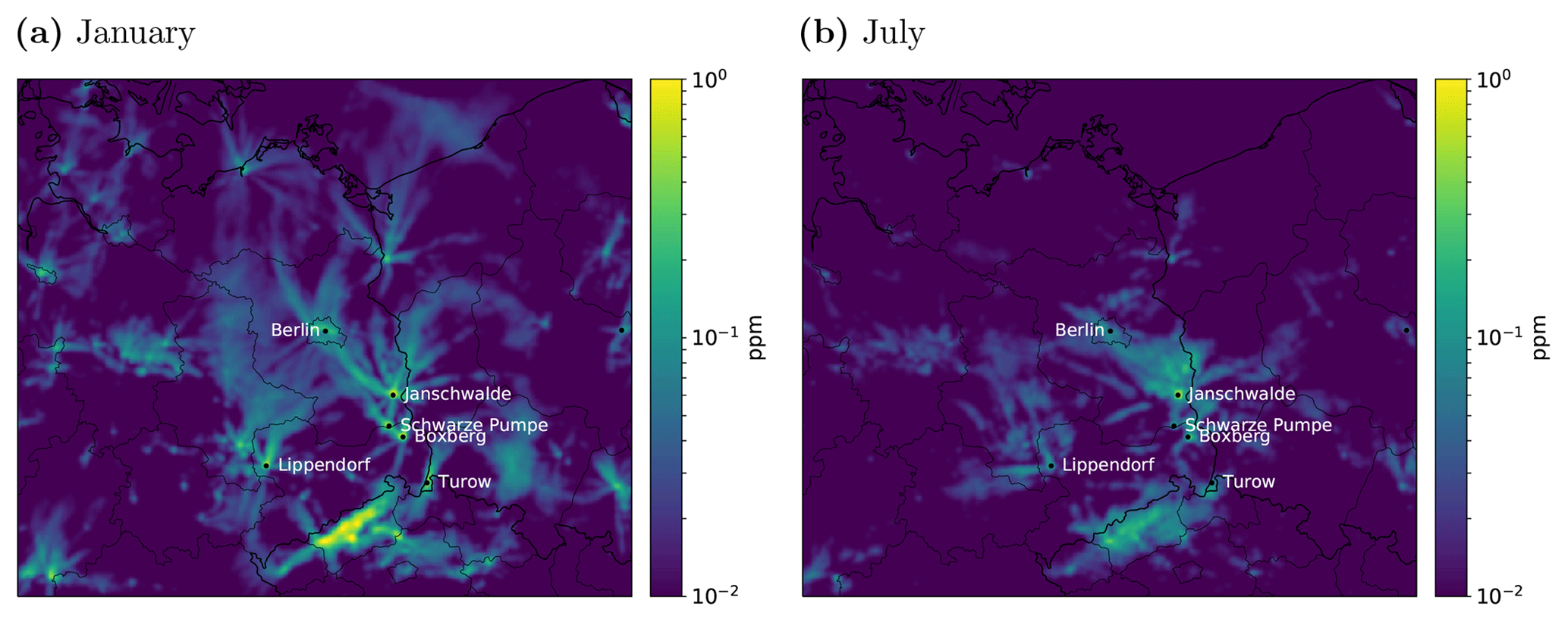
Figure 10 Difference in 11:30 LT column-averaged dry air mole fractions (XCO₂) between tracers CO2_SURF and CO2_VERT in (a) January and (b) July.

Maps of XCO₂ and of the differences between the two tracers are presented in Figs. 9 and 10 in the same way as for the surface concentrations. Instead of presenting mean afternoon values, the figures show the situation at 11:30 LT (the average of output at 10:00 and 11:00 UTC) corresponding to the expected overpass time of the planned European satellites. Note that we did not account for daylight savings time in the diurnal cycles of emissions but assumed a constant offset of +1 h between local time in the domain and UTC. Differences in XCO₂ between the two tracers are indeed much smaller than the differences in surface concentrations, suggesting that total column observations are much less sensitive to the vertical placement of emissions. However, differences are not negligible, especially in winter (Fig. 10). The largest differences in January are seen in the northern parts of Czech Republic, which is the main coal-mining region of the country featuring a large number of power plants. Since plume rise was not explicitly calculated, CO2_VERT emissions from these power plants followed the EMEP profiles, which tend to place emissions too high, as mentioned earlier. Differences over the power plants with explicit plume rise are smaller, but not negligible, with values around 1 ppm close to the sources.

Domain-averaged mean diurnal cycles are presented in Fig. 11 and overall statistics in Table 4. Similar to the results for near-surface concentrations, the differences are larger in winter than in summer. In contrast to the situation at the surface, the differences in XCO₂ remain fairly constant over the day not only in winter but also in summer. Relative differences in mean XCO₂ are only 7.7 % in January (compared to 43 % at the surface) and 4.8 % in July (compared to 14 % at the surface). Note that the differences in the columns are related to the synthetic nature of our model experiment, since no anthropogenic CO₂ emissions are advecting into the domain from sources outside. Nevertheless, the analysis reveals significant differences in the contributions from sources within the domain, which is the information used by any regional inverse modeling system. Consistent with the findings for near-surface concentrations, the differences tend to increase for higher percentiles, reaching about 10 % at the 95th percentile (see last column in Table 4).

Table 4 Statistics of near-surface CO₂ and column-averaged dry air mole XCO₂ fractions in the model domain for the tracers CO2_VERT and CO2_SURF. Differences are presented in terms of (CO2_SURF-CO2_VERT)/CO2_VERT.

Although differences in monthly mean XCO₂ values are relatively small, the differences can be very large at a given location and time, as illustrated in Fig. 12 for 2 July 2015. The figure shows the differences in XCO₂ between two CO₂ tracers representing emissions from the largest power plants in the domain. The two tracers were released either using explicit plume rise simulations (CO2_PP-PR) or according to EMEP SNAP 1 profiles (CO2_PP-EMEP). No power-plant-only tracer was simulated with emissions at the surface. Plume rise was rather moderate (to about 340 m above ground) at this time due to pronounced easterly winds. The red (positive) parts in the figure correspond to plumes produced by CO2_PP-PR, whereas the blue parts (negative) correspond to the tracer CO2_PP-EMEP.

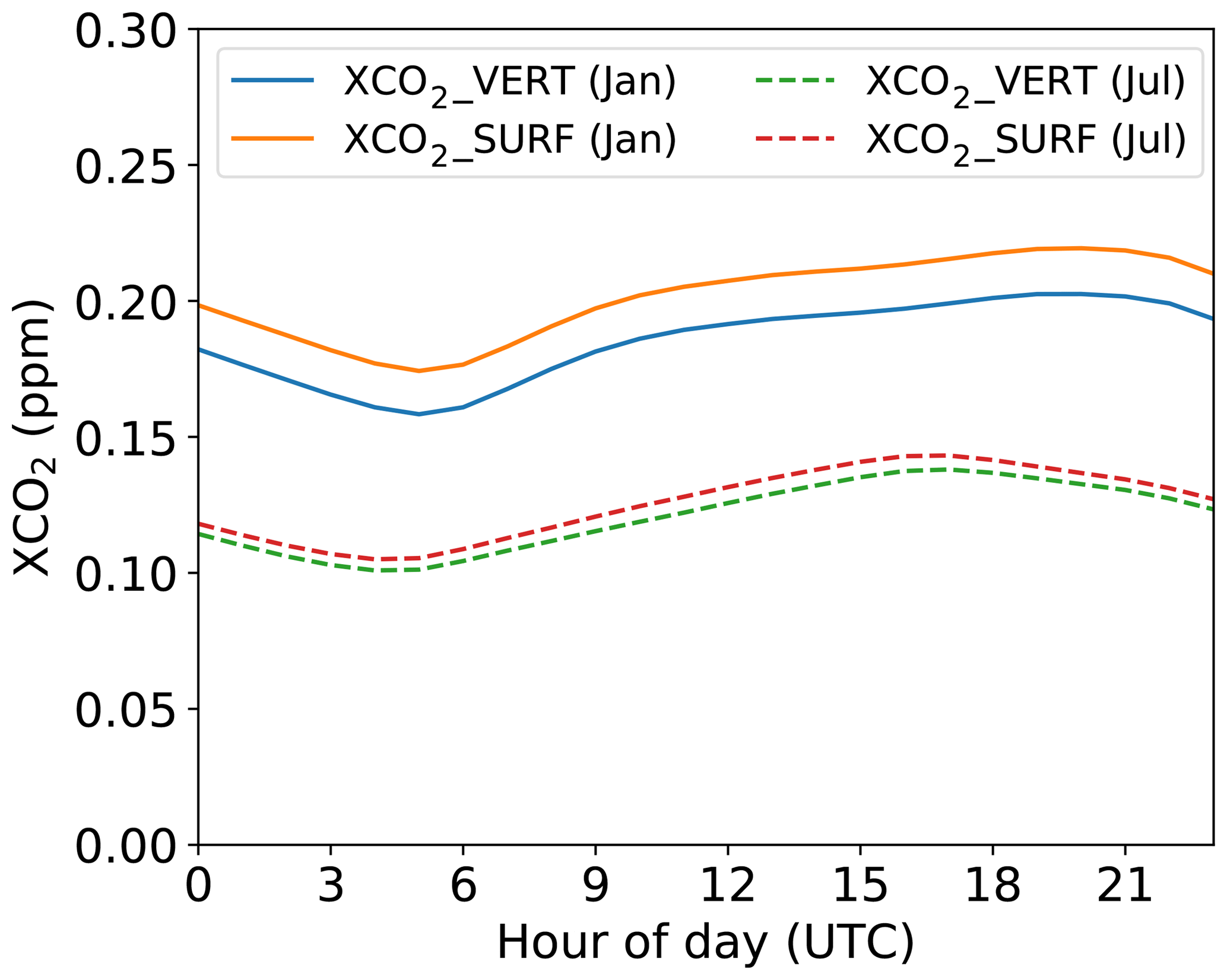
Figure 11 Mean diurnal cycles of column-averaged dry air mole fractions (XCO₂) of the tracers CO2_VERT and CO2_SURF in January and July.

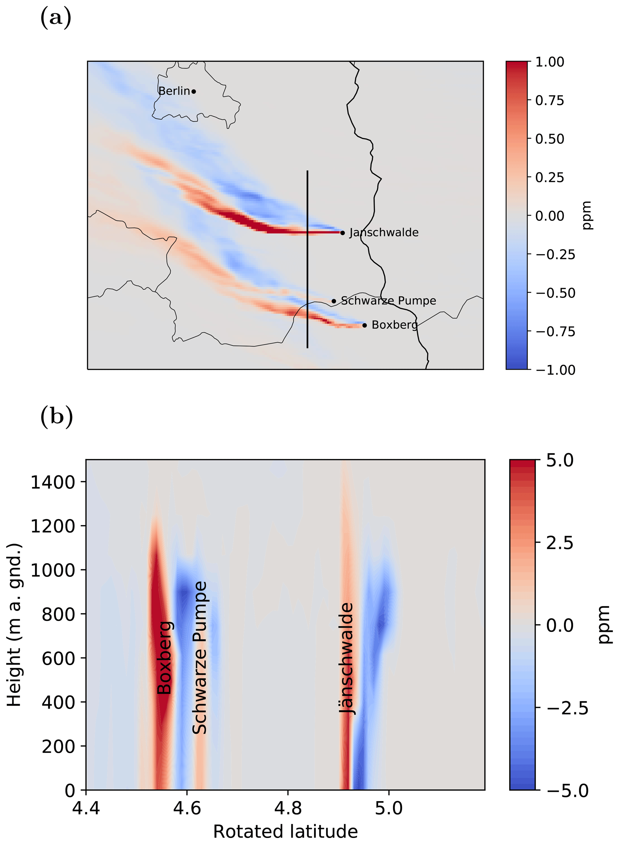
Figure 12 Difference on 2 July 2015 11:00 LT between power plant CO₂ tracer with explicit plume rise (CO2_PP-PR) and released according to standard EMEP SNAP 1 profile (CO2_PP-EMEP). (a) Map of the difference in column-averaged dry air mole XCO₂ fractions. (b) Vertical cross-section of the difference in CO₂ along the transect indicated in panel (a). The length of this cross-section is about 100 km.

Due to wind directions changing with altitude and due to the different emission heights of the tracers, the plumes are transported in different directions. Spiraling wind directions are typical of the boundary layer where winds near the surface have an ageostrophic, cross-isobaric component due to surface friction, while winds become increasingly geostrophic at higher levels. This is known as the Ekman spiral. The plumes of CO2_PP-EMEP show a stronger lateral dispersion because the tracer is released over a large vertical extent (blue line in Fig. 2). The vertical cross-section transecting the plumes about 15 to 30 km downwind of the sources suggests that both tracers are partially mixed over the full depth of the boundary layer at this distance, but that the centers of the plumes are clearly higher above the surface for the tracer CO2_PP-EMEP than for CO2_PP-PR.

4 Discussion

The results for near-surface concentrations revealed a strong sensitivity to the vertical placement of emissions, especially in winter. Similarly large sensitivities were reported for air pollution simulations. By conducting a set of five 1-year European-scale model simulations differing only in the vertical allocation of emissions, Mailler et al. (2013) found that ground-based concentrations of SO₂, an air pollutant primarily released by point sources, increased on average by about 70 % when reducing all emission heights by a factor of 4. The changes were less significant (about 15 %) for NO₂ due to the larger contribution from traffic emissions. Sensitivities of a similar magnitude were reported by Guevara et al. (2014) for simulations over Spain when replacing the EMEP profiles for power plants by more realistic plume rise calculations.

The results of the present study may be considered as upper limits of the sensitivity for two reasons. First of all, our simulations covered a region in Europe with a particularly high density of coal-fired power plants. Simulations over other regions such as France, where electricity is mostly produced by nuclear power, would likely have yielded lower sensitivities. Nevertheless, averaged over Europe, large point sources are responsible for at least half of all anthropogenic CO₂ emissions (52 % in 2011) according to the TNO/MACC-3 inventory, which underscores the general importance of properly allocating their emissions vertically.

Second, for most point sources in our domain, the standard EMEP profiles were applied, which tend to place emissions too high in the atmosphere as suggested consistently by Bieser et al. (2011); Guevara et al. (2014); Mailler et al. (2013) and by our own comparison with explicit plume rise simulations. Several improvements were already implemented in the present study, each of them leading to a reduction of the effective emission heights and likely to a more realistic representation as compared to EMEP. This included a modification of SNAP 9 profiles, the distinction between point and area sources, and the explicit computation of plume rise for the largest sources in the domain. Due to a lack of representative studies, these modifications were somewhat arbitrary. More studies like Bieser et al. (2011) and Pregger and Friedrich (2009) are needed, but should not only target large point sources but also emissions from the remaining 48 % of emissions, including residential heating, even though their vertical placement will be less critical. Explicit plume rise computations for all large point sources as performed in some air quality models (Karamchandani et al., 2014) would be the best alternative to using static profiles, but this adds significant complexity to the model, and individual stack and flue gas parameters are not publicly available in Europe (Pregger and Friedrich, 2009).

None of the studies mentioned above considered the issue of interaction between multiple plumes and latent heat release in cooling tower plumes, which tend to enhance plume rise. The SNAP 1 profiles recommended by Bieser et al. (2011) and the simulations conducted here are only representative of isolated stacks, which is not consistent with any of the German coal-fired power plants in our domain. Comprehensive models for plume rise from single and multiple interacting cooling tower plumes have been presented by Schatzmann and Policastro (1984) and Policastro et al. (1994), but they seem not to be widely applied, although the code of Schatzmann and Policastro (1984) is available through the Association of German Engineers (VDI; https://www.vdi.de/index.php?id=4791, last access: 26 March 2019). Most plume rise studies date back 20 to 50 years, and modern computational fluid dynamics simulations are lacking, with the exception of the study of Bornoff and Mokhtarzadeh-Dehghan (2001) on the interaction of plumes from two adjacent cooling towers.

Mean afternoon differences at the surface in January between the tracers CO2_VERT and CO2_SURF are of the order of 1.5 ppm, which is close to 50 % of the total anthropogenic CO₂ signal due to emissions within the model domain. In summer, the relative differences in the afternoon are much smaller due to more efficient vertical mixing but still as large as 14 %. Inaccurate vertical placement of the emissions may thus lead to biases of a magnitude comparable to other error sources reported in the literature. Random uncertainties around 30 %–50 % of the regional biospheric CO₂ signal have been estimated, for example, for model errors in PBL mixing (Gerbig et al., 2008) and in wind speed and direction (Lin and Gerbig, 2005). Systematic biases in simulated near-surface wind speeds of mesoscale weather prediction models like COSMO or WRF are typically on the order of 0.5–1 m s⁻¹ or about 10 %–20 % of the mean wind speeds (Jiménez and Dudhia, 2012; Brunner et al., 2015; Bagley et al., 2018), which may translate into similar biases in near-surface concentrations. Systematic differences in emission estimates using different regional transport and inverse modeling systems were reported to be around 20 %–40 % (Hu et al., 2014; Bergamaschi et al., 2018b). Our analysis focused on the situation in the lowest model layer at 0–20 m. However, the recommended strategy for CO₂ monitoring is to sample from tall towers well above the surface. At higher elevations, the model sensitivity to the vertical placement of emissions is likely smaller, which is another benefit of tall tower measurements in addition to their greater spatial representativeness.

Mean differences in total column XCO₂ between the tracers CO2_VERT and CO2_SURF are much smaller, around 8 % in winter and 5 % in summer. However, differences are larger at the highest percentiles (about 10 % at the 95 % percentile), which are more relevant for satellite missions like Sentinel-CO₂ designed to image individual plumes. Furthermore, the vertical placement of emissions has a significant effect on the speed and direction of individual plumes, suggesting that an accurate vertical placement is a critical requirement for inverse modeling of power plant emissions from satellite observations. Irrespective of a correct vertical placement of emissions, an appropriate simulation of power plant plumes will remain a great challenge for any mesoscale atmospheric transport model. Current approaches for estimating power plant emissions are circumventing this problem by directly matching the “observed” wind direction defined by the location of the plume, e.g., by fitting a Gaussian plume model (Krings et al., 2018; Nassar et al., 2017). However, these methods also need to make a realistic assumption about the height of the plume, since the mean advection speed of the plume needs to be estimated from a simulated or observed vertical wind profile.

5 Conclusions

We investigated the sensitivity of model-simulated near-surface and total column CO₂ concentrations to a realistic vertical allocation of anthropogenic emissions as opposed to the traditional approach of emitting CO₂ only at the surface. The study was conducted using kilometer-scale atmospheric transport simulations for the year 2015 for a domain covering the city of Berlin and numerous power plants in Germany, Poland and Czech Republic. More than 50 % of CO₂ in Europe is emitted from large point sources, mostly through stacks and cooling towers, suggesting that a proper representation of these sources in the vertical dimension may be critical. Our results indeed confirm a strong sensitivity of near-surface afternoon concentrations: a regional CO₂ tracer released in the model domain only at the surface was on average 43 % higher in winter and 14 % higher in summer than a tracer released according to realistic vertical profiles. Since measurements of CO₂ are often taken from towers some 100 to 300 m above the surface (Bakwin et al., 1995), the impact on actual ground-based observations will likely be somewhat smaller.

Differences were smaller but not negligible (5 %–8 %) for total column XCO₂, suggesting that the assimilation of satellite observations is less sensitive to the vertical placement of emissions than the assimilation of ground-based observations. Individual plumes as imaged by future CO₂ satellites, however, may propagate more rapidly and in different directions when using realistic vertical profiles instead of releasing CO₂ only at the surface.

Plume rise was explicitly simulated for the six largest power plants in the domain and for the 22 largest point sources in Berlin. Power plant plumes typically rose between 100 and 400 m above the top of the stacks. Plume rise showed significant seasonal and diurnal variability that would be missed when applying static vertical profiles. Simulated plume rise was on average more than 100 m lower than suggested by the frequently used EMEP profile for power plant emissions. An accurate vertical placement of emissions is not only critical for power plants but may also be relevant for the simulation of city plumes. In the case of Berlin, for example, more than 35 % of CO₂ is released through stacks presumably more than 90 m above surface.

We strongly recommend the representation of CO₂ emissions in all three dimensions in regional atmospheric transport and inverse modeling studies. The specific impact on the model results will depend on factors such as vertical model resolution and boundary layer scheme but in general cannot be expected to be negligible. Current gridded emission inventories only provide information in two dimensions. Information on the source-specific vertical allocation of emissions as used in this study, conversely, is still sparse and should receive more attention in the future.