Quantifying the UK's carbon dioxide flux: an atmospheric inverse modelling approach using a regional measurement network

We present a method to derive atmospheric-observation-based estimates of carbon dioxide (CO₂) fluxes at the national scale, demonstrated using data from a network of surface tall-tower sites across the UK and Ireland over the period 2013–2014. The inversion is carried out using simulations from a Lagrangian chemical transport model and an innovative hierarchical Bayesian Markov chain Monte Carlo (MCMC) framework, which addresses some of the traditional problems faced by inverse modelling studies, such as subjectivity in the specification of model and prior uncertainties. Biospheric fluxes related to gross primary productivity and terrestrial ecosystem respiration are solved separately in the inversion and then combined a posteriori to determine net ecosystem exchange of CO₂. Two different models, Data Assimilation Linked Ecosystem Carbon (DALEC) and Joint UK Land Environment Simulator (JULES), provide prior estimates for these fluxes. We carry out separate inversions to assess the impact of these different priors on the posterior flux estimates and evaluate the differences between the prior and posterior estimates in terms of missing model components. The Numerical Atmospheric dispersion Modelling Environment (NAME) is used to relate fluxes to the measurements taken across the regional network. Posterior CO₂ estimates from the two inversions agree within estimated uncertainties, despite large differences in the prior fluxes from the different models. With our method, averaging results from 2013 and 2014, we find a total annual net biospheric flux for the UK of 8±79 Tg CO₂ yr⁻¹ (DALEC prior) and 64±85 Tg CO₂ yr⁻¹ (JULES prior), where negative values represent an uptake of CO₂. These biospheric CO₂ estimates show that annual UK biospheric sources and sinks are roughly in balance. These annual mean estimates consistently indicate a greater net release of CO₂ than the prior estimates, which show much more pronounced uptake in summer months.

1 Introduction

There are significant uncertainties in the magnitude and spatiotemporal distribution of global carbon dioxide (CO₂) fluxes to and from the atmosphere, particularly those due to terrestrial ecosystems (Le Quéré et al., 2018). Reliable methods for quantifying carbon budgets at policy-relevant scales (i.e. national or subnational) will be important to accurately and transparently evaluate each country's progress towards achieving their Nationally Determined Contributions (NDCs) made following the Paris Agreement (UNFCCC, 2015).

Regional terrestrial carbon fluxes can be estimated using a range of observational, computational and inventory-based methods. These include bottom-up approaches such as the upscaling of direct flux measurements made using eddy covariance or chamber systems (Baldocchi and Wilson, 2001) and models of atmosphere–biosphere CO₂ exchange. Flux measurements are important for understanding the small-scale processes responsible for carbon fluxes. However, they are relatively localised estimates (metres to hectares), which are challenging to scale up to national levels. Biosphere models and land surface models can be used to estimate carbon fluxes using coupled representations of biogeophysical and biogeochemical processes, driven by observations of meteorology and ecosystem parameters (Potter, 1999; Clark et al., 2011; Bloom et al., 2016). Such models describe processes to varying degrees of complexity, with poorly described errors, and are driven by observational data at differing temporal and spatial resolutions; hence predictions of biogenic greenhouse gas (GHG) fluxes have poorly quantified biases and can vary significantly between models (Todd-Brown et al., 2013; Atkin et al., 2015).

Atmospheric inverse modelling is a top-down approach that provides an alternative to the bottom-up approaches. Inversions have been used to indirectly estimate country-scale (e.g. Matross et al., 2006; Schuh et al., 2010; Meesters et al., 2012) and continental (e.g. Gerbig et al., 2003; Peters et al., 2010; Rivier et al., 2010) biospheric CO₂ budgets using atmospheric mole fraction observations, where the contribution of anthropogenic fluxes to the observations has been removed. In this approach, a model of atmospheric transport relates spatiotemporally resolved surface fluxes of biospheric CO₂ to atmospheric measurements of CO₂ mole fractions. Biospheric fluxes derived from bottom-up approaches are often used as prior estimates in the inversion. Since atmospheric observations are sensitive to fluxes spanning tens to hundreds of kilometres (Gerbig et al., 2009), inverse methods are a valuable tool for examining national fluxes and evaluating estimates of surface exchange of CO₂ at larger spatial scales. However, errors in atmospheric transport, unknown uncertainties related to the prior fluxes and issues surrounding the underdetermined nature of the problem are all limitations of this approach.

The United Kingdom (UK) government has set legally binding targets to curb GHG emissions in an attempt to prevent dangerous levels of climate change. The Climate Change Act 2008 (UK government, 2008) commits the UK to 80 % cuts in GHG emissions, from 1990 levels, by 2050. To support this legislation, a continuous and automated measurement network has been established (Stanley et al., 2018; Stavert et al., 2018) with the goal of providing estimates of GHG emissions using methods that are complementary to those used to compile the UK's bottom-up emissions inventory, reported annually to the United Nations Framework Convention on Climate Change (UNFCCC). Previous studies have used data from the UK Deriving Emissions related to Climate Change (UK-DECC) network to infer emissions of methane, nitrous oxide and HFC-134a from the UK (Manning et al., 2011; Ganesan et al., 2015; Say et al., 2016). These studies found varying levels of agreement with bottom-up inventory methods, where estimates of GHG emissions are made using reported statistics from various sectors (e.g. road transport, power generation). Here we use the DECC network and two additional sites from the Greenhouse gAs Uk and Global Emissions (GAUGE) programme (Palmer et al., 2018) to estimate biospheric fluxes of CO₂. Whilst anthropogenic emissions, which are the remit of the UK inventory, are not estimated in this study, these biospheric estimates represent the first step towards a framework for estimating the complete UK CO₂ budget.

Atmospheric inverse modelling of GHGs using Bayesian methods presents some known challenges. Robust uncertainty quantification in Bayesian frameworks can be difficult as they require that uncertainties in the prior flux estimate, and uncertainties in the atmospheric transport model's ability to simulate the data, are well characterised. In practice, this is rarely the case because, for example, uncertainties related to the atmospheric transport model are poorly understood and uncertainties related to biospheric flux estimates from models are largely unknown. Various studies have investigated the use of data-driven uncertainty estimation (Michalak, 2004; Berchet et al., 2013; Ganesan et al., 2014; Kountouris et al., 2018b). Inversions are also known to suffer from aggregation errors. One type of aggregation error arises from the way in which areas of the flux domain are grouped together to decrease the number of unknowns, because usually there are not sufficient data to solve for fluxes in each model grid cell (Kaminski et al., 2001). Furthermore, for reasons of mathematical and computational convenience, Gaussian probability density functions (PDFs) are commonly used to describe prior knowledge (e.g. Miller et al., 2014). However, Gaussian assumptions can lead to unphysical solutions in the case of atmospheric GHG emissions or uptake processes, as they permit both positive and negative solutions.

CO₂ presents further complications over other GHGs in that atmosphere–biosphere CO₂ exchange has a diurnal flux cycle that is significantly larger than the net flux and has strong, spatially varying surface sources and sinks. Gerbig et al. (2003) was one of the first to develop an analysis framework for regional-scale CO₂ flux inversions. The study sets out the need to explicitly simulate the diurnal cycle of biospheric fluxes and highlights the importance of high spatial and temporal resolution data when addressing the unique problems of representation and aggregation errors caused by the highly varying nature of CO₂ fluxes in both space and time. Inverse modelling studies of CO₂ flux typically assume that anthropogenic fluxes are “fixed” in the inversion (e.g. Meesters et al., 2012; Kountouris et al., 2018a). This is based on the assumption that uncertainties in anthropogenic fluxes are low compared to those of the biospheric fluxes. However, it has been suggested that this may not necessarily be the case (Peylin et al., 2011).

Here we outline a framework for evaluating the net biospheric CO₂ exchange (net ecosystem exchange, NEE) from a small- to medium-sized country (the UK covers an area of around 250 000 km²) using the high-resolution regional, Lagrangian transport model, the Numerical Atmospheric dispersion Modelling Environment (NAME, Jones et al., 2006). To address many of the problems outlined above, we use an adapted form of a hierarchical Bayesian, trans-dimensional Markov chain Monte Carlo (MCMC) inversion (Rigby et al., 2011; Ganesan et al., 2014; Lunt et al., 2016). In the hierarchical Bayesian framework presented in Ganesan et al. (2014), “hyperparameters” that define the prior flux and model–data “mismatch” uncertainty PDFs are included in the inversion, which is solved using a Metropolis–Hastings MCMC algorithm (e.g. Rigby et al., 2011). This hierarchical approach has been shown to lead to more robust posterior uncertainty quantification in Bayesian frameworks where prior uncertainties are not well characterised (Ganesan et al., 2014). Lunt et al. (2016) built on this method, developing a “trans-dimensional” framework that accounted for the uncertainty in the definition of basis functions (the way in which flux grid cells are aggregated) and allowed this to propagate through to the posterior estimate.

Gross primary productivity (GPP) and terrestrial ecosystem respiration (TER) estimates from the Joint UK Land Environment Simulator (JULES) and Data Assimilation Linked Ecosystem Carbon (DALEC) models are used as prior flux constraints. JULES is a state-of-the-art physically based, process-driven model that estimates the energy, water and carbon fluxes at the land–atmosphere boundary and uses a variety of observation-derived products describing physical parameters as inputs (Best et al., 2011; Clark et al., 2011). DALEC, on the other hand, is a simplified terrestrial C-cycle model which is calibrated independently at each location retrieving both process parameters and initial conditions using the carbon data model framework (CARDAMOM) model–data fusion system. CARDAMOM ingests satellite-based remotely sensed estimates of the state of terrestrial ecosystems (Bloom and Williams, 2015; Bloom et al., 2016; Smallman et al., 2017).

Below, we first describe our approach for modelling biospheric CO₂ fluxes, including several novel aspects compared to previous work in this area. We then investigate the impact of using two different models that simulate biospheric fluxes (JULES and DALEC) within our proposed inverse framework and discuss the discrepancies between the prior and posterior flux estimates.

2 Method

The main components of a regional atmospheric inverse modelling framework are the atmospheric CO₂ mole fraction data themselves, a model of atmospheric transport including a set of boundary conditions at the edge of the regional domain and some initial information or “first guess” of regional CO₂ fluxes. These components are combined in an inversion set-up with a mechanism for dealing with uncertainties in the inputs. To make the problem computationally manageable, the regional domain is often decomposed into a number of basis functions, describing a spatial grouping of grid cells within which fluxes are scaled up or down. The selection of these basis functions constitutes a further key element of the atmospheric inverse problem.

2.1 Site location and measurements

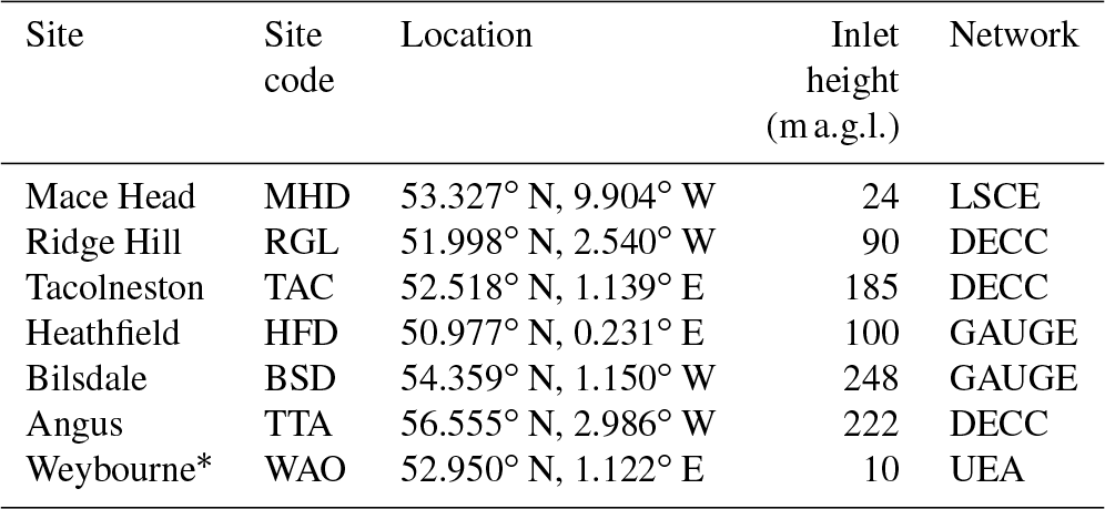
This study focuses on the years 2013 and 2014. During this period, atmospheric CO₂ mole fractions were continuously measured at six sites across the UK and Republic of Ireland (see Table 1 for site information and Fig. 1 for the location of the sites). Four of these sites originally formed the UK-DECC network and are described in Stanley et al. (2018), whilst two were developed under the GAUGE programme and are described in Stavert et al. (2018). The site at Mace Head, Republic of Ireland, is a coastal, 10 m a.g.l. (above ground level), station situated primarily to measure concentrations of background air arriving at the site from the Atlantic Ocean. The Laboratoire des Sciences du Climat et de l'Environnement (LSCE) is responsible for making CO₂ measurements at this site from a 23 m a.g.l. inlet (see Vardag et al., 2014, for a full site description). All of the UK sites are tall-tower stations (with inlets ranging from 42 to 248 m a.g.l.), designed to measure elevated GHG mole fractions as air is transported over the surface in the UK and Europe.

Figure 1 Mean annual NAME footprint for 2014, for each of the six sites. MHD: Mace Head; RGL: Ridge Hill; HFD: Heathfield; TAC: Tacolneston; BSD: Bilsdale; TTA: Angus. WAO shows the location of the Weybourne Atmospheric Observatory, where data have been used to validate the results but have not been included in the inversion (the mean footprint from this station is not plotted).

Continuous CO₂ measurements are made at all stations using cavity ring-down spectrometers (CRDS: Picarro G2301 or G2401). CRDS data are corrected for daily linear instrumental drift using standard gases and for instrumental non-linearity using calibration gases, spanning a range of above and below ambient mole fractions, on a monthly basis (Stanley et al., 2018). Calibration and standard gases are of natural composition and calibrated at the GasLab, Max Planck Institute for Biogeochemistry, Jena, or the World Calibration Centre for CO₂ at Empa, linking them to the World Meteorological Organisation (WMO) X2007 scale (Stanley et al., 2018; Stavert et al., 2018). At sites with multiple inlets, measurements are taken for the same length of time at each inlet, each hour. This means that measurements at each height at Bilsdale and Tacolneston (with three inlets) are taken continuously for roughly 20 min every hour, and at Heathfield and Ridge Hill (with two inlets) measurements are taken continuously for roughly 30 min at each inlet every hour. For the purposes of the inverse modelling carried out in this study, the continuous CRDS data are used from the highest inlets and averaged to a 2 h time resolution. Further information about the instruments, measurement protocol and uncertainty estimates can be found in Stanley et al. (2018) and Stavert et al. (2018).

2.2 Atmospheric transport model

In this work we use a Lagrangian particle dispersion model (LPDM), NAME, which tracks thousands of particles back in time from observation locations. The model determines the locations where air masses interacted with the surface and therefore where surface CO₂ sources and sinks could contribute to a CO₂ concentration measurement. The model provides a gridded sensitivity of each mole fraction observation to the potential flux from each grid cell and this is often referred to as the “footprint” of a particular observation (for further details, see e.g. Manning et al., 2011).

Table 1 Measurement site information. The location of sites is also shown in Fig. 1. ^* Weybourne data were used for validation of the results only and were not included in the inversions. LSCE – Laboratoire des Sciences du Climat et de l'Environnement; DECC – Deriving Emissions related to Climate Change; GAUGE – Greenhouse gAs Uk and Global Emissions; UEA – University of East Anglia.

At each 2-hourly measurement time step, the model releases 20 000 particles, which are tracked back in time for 30 days, so that by the end of this period the majority of particles will have left the model domain (Fig. S1 in the Supplement). Since most CO₂ flux to the atmosphere occurs at the surface, we record the instances where the particles are in the lowest 40m of the atmosphere and assume that this represents the sensitivity of observed mole fractions to surface fluxes in the inversion domain. The domain used to calculate atmospheric transport covers most of Europe, the east coast of North and Central America, and North Africa (10.729–79.057^∘ N and 97.9^∘ W–39.38^∘ E). The spatial resolution of the meteorological analysis dataset used to drive the model, from the Met Office Unified Model (Cullen, 1993), was 0.233^∘ by 0.352^∘ (roughly 25 km by 25 km over the UK).

In many previous inverse modelling studies using LPDMs (e.g. Manning et al., 2011; Thompson and Stohl, 2014; Steinkamp et al., 2017) the footprint is assumed to be equal to the integrated air history over the duration of the simulation (e.g. 30 days, as in Fig. 1). Based on the assumption that fluxes have not changed substantially during the 30-day period, the integrated footprint can be multiplied by the prior flux and summed over all the grid cells in the domain to create a time series of modelled mole fractions at each measurement site. However, many CO₂ inverse modelling studies using other LPDMs have disaggregated footprints back in time, capturing changes in surface sensitivity on timescales shorter than the duration of the simulation, thereby attempting to account for diurnal variation in CO₂ fluxes (Denning et al., 1996; Gerbig et al., 2003; Gourdji et al., 2010). Thus far, a disaggregation such as this has not been used in NAME simulations, so we describe our method here.

In our simulations, we determined the footprint for 2-hourly average periods back in time for the first 24 h before the observation and then replaced the first 24 h of integrated sensitivities with these time-disaggregated footprints. Mole fractions were simulated by multiplying these footprints by biospheric flux estimates for the corresponding time, so that the variability in the source or sink of CO₂ was represented in the modelled observations. This is demonstrated in Eq. (1), which yields the modelled mole fraction, y_t, for one 2-hourly measurement time step, t, at one measurement site.

$$\begin{array}{}\text{(1)}& {\displaystyle }{\displaystyle }{y}_t=\sum _{i=\mathrm{0}}^{\mathrm{12}}\sum _{j=\mathrm{0}}^n{\mathrm{fp}}_{t-i,j}\times q_{t-i,j}+\sum _{j=\mathrm{0}}^n{\mathrm{fp}}_{{\mathrm{remainder}}_j}\times q_{{\mathrm{month}}_j}\end{array}$$

Here i denotes the number of 2 h periods back in time before the particle release at time t; j represents the grid cell where n is the maximum number of grid cells; fp${}_{t-i,j}$ is one grid cell of the two-dimensional time-disaggregated footprint for that time; $q_{t-i,j}$ is one grid cell of the two-dimensional, 2-hourly flux field corresponding to the time the particles were interacting with the surface; fp_remainder is the remaining 29-day footprint; and q_month is the monthly average flux. The choice of 24 h disaggregation balanced considerations of computational efficiency and simulation accuracy. For certain months and sites we carried out a set of tests to determine how sensitive our simulated mole fractions and inversion results were when footprints were disaggregated for the first 12 or 72 h prior to each measurement (Fig. S2; Table S1 in the Supplement). Assuming that the 72 h simulations were the most accurate, we found little degradation in performance by using only 48 or 24 h disaggregation, when compared to the other uncertainties in the system (e.g. differences between fluxes derived using the 24, 48 and 72 h simulations were smaller than the 90 % confidence interval). However, when only 12 h was used (or fully integrated footprints), the modelled diurnal cycle was out of phase with the observations.

2.2.1 Data selection and model uncertainty

LPDMs are known to perform poorly under certain meteorological conditions. In particular, it is often assumed that model–data mismatch should be smallest during periods when the boundary layer is relatively well mixed. A common approach is to only include daytime data in the inversion (e.g. Meesters et al., 2012; Steinkamp et al., 2017; Kountouris et al., 2018a) or separate morning and afternoon averages (e.g. Matross et al., 2006). To make use of as much high-frequency-measurement information as possible, we use a filter based on two metrics to remove times of high atmospheric stability and/or stagnant conditions. The first metric is based on calculating the ratio of the NAME footprint magnitude in the 25 grid boxes in the immediate vicinity of the measurement station to the total for all of the grid boxes in the domain. A high ratio indicates times when a significant fraction of air influencing the observation point originates from very local sources, which may not be resolved by the model (Lunt et al., 2016). The second metric is based on the modelled lapse rate at each site, which is a measure of atmospheric stability. A high lapse rate suggests very stable conditions, which would be conducive for significant local influence. Thresholds for each of these criteria were chosen to preserve as much data as possible, whilst retaining only points that the model was (somewhat subjectively) found to resolve well. In practice, the filter retained many more daytime than night-time points (see Fig. S3 for an analysis of the data removed in 2014) and inversion results were mostly similar to when only daytime data were used; however, differences were seen in some months when stagnant conditions occurred for several daytime periods (Fig. S4).

Model uncertainty (or model–data mismatch) has a measurement uncertainty component and a component that takes into account the ability of the model to represent real atmospheric conditions. The measurement uncertainty was assumed to be equal to the standard deviation of the measurements over the 2 h period to give an estimate of measurement repeatability and a measure of the sub-model-timescale variability in the observations. The 2-hourly measurement uncertainty was then averaged over the month to ensure that measurements of high concentrations were not de-weighted, as they are more likely to have greater variability and therefore a larger standard deviation. Monthly average measurement uncertainty is around 0.9 ppm. The measurement uncertainty is combined with a range of prior values for model uncertainty (as this is a poorly constrained quantity), and together the model–measurement uncertainty is one of the hyper-parameters solved in the inversion (further explained in Sect. 2.4.1).

Table 2 Specifications for different prior and fixed fluxes.

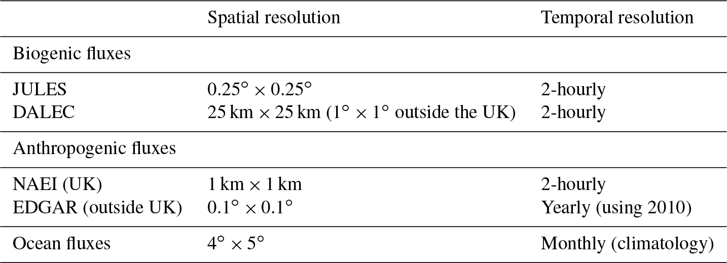
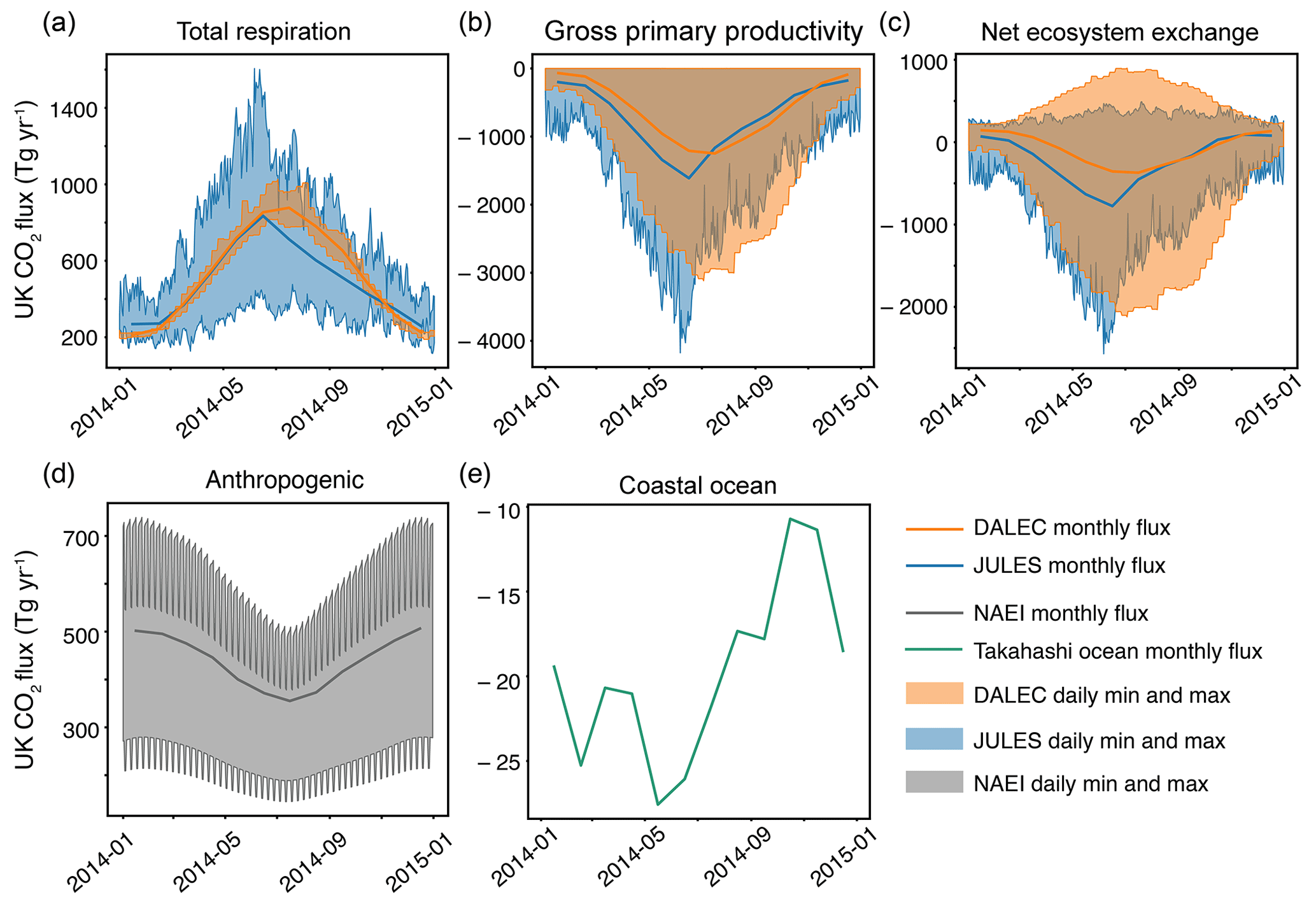
Figure 2 Prior UK fluxes in 2014. (a–c) Comparison of JULES (blue) and DALEC (orange) monthly fluxes and minimum and maximum daily values for TER, GPP and NEE respectively. (d) Monthly anthropogenic fluxes and minimum and maximum daily values from the NAEI inventory within the UK. (e) Monthly coastal ocean net fluxes from the Takahashi et al. (2009) ocean CO₂ flux product.

2.2.2 Boundary conditions

The footprints from the LPDM only take into consideration the influence on the observations of sources intercepted within the model domain. Therefore, an estimate of the mole fraction at the boundary must be made and incorporated into the simulated mole fractions. To estimate spatial and temporal gradients in these boundary conditions we use the global Eulerian Model for OZone And Related chemical Tracers (MOZART, Emmons et al., 2010). The model was run using GEOS-5 meteorology (Rienecker et al., 2011) and global biospheric fluxes from the NASA-CASA biosphere model (Potter, 1999), global ocean fluxes from Takahashi et al. (2009) and global anthropogenic fluxes from the Emission Database for Global Atmospheric Research (EDGAR, EC-JRC/PBL, 2011). When particles leave the NAME model domain, we record the time and location of the exit point. We then use MOZART to find the concentration of CO₂ at these locations to serve as prior boundary conditions. The global MOZART initial mole fraction field for January 2014 was scaled before commencing the 2014 MOZART run to match the surface South Pole value to the mean NOAA January 2014 flask value (Dlugokencky et al., 2018). This scaling factor was also applied to any pre-January 2014 MOZART output to prevent any discontinuities in the boundary mole fraction fields. The mole fraction at each domain edge (N, E, S, W) is then scaled up or down during the inversion to account for uncertainties in the MOZART boundary conditions (Lunt et al., 2016). A sensitivity test where 1 ppm is added or taken away from the mole fractions at the domain edges indicates that in June a ±1 ppm change translates to a 1 %–3 % change in the inversion result and in December a ±1 ppm change translates to a 7 %–11 % change in the inversion result. These changes are substantially smaller than the posterior uncertainty.

2.3 Prior information

In this work, we used model analyses to provide prior information about biospheric fluxes. Two models (DALEC and JULES) were used to assess how much influence the choice of biospheric prior has on the outcome of the inversion. The NAME model was used to simulate the contribution of anthropogenic and oceanic fluxes to the data, and this contribution was removed from the observations prior to the inversion. The fluxes used for this calculation are described below. The spatial and temporal resolution of the prior information and fixed fluxes are summarised in Table 2 and emissions from each source over the UK are shown in Fig. 2.

In a synthetic data study in which biospheric CO₂ was inferred, Tolk et al. (2011) found that separately solving for positive fluxes (autotrophic and heterotrophic respiration combined, TER) and negative fluxes (GPP) in atmospheric inversions provided a better fit to the atmospheric mole fraction data than inversions that scaled NEE only. Equation (2) describes the relationship between these three variables:

$$\begin{array}{}\text{(2)}& {\displaystyle }{\displaystyle }\mathrm{NEE}=\mathrm{TER}-\mathrm{GPP}.\end{array}$$

This separation has been applied in various studies demonstrating model set-ups with synthetic data, for example geostatistical approaches (Göckede et al., 2010), ensemble Kalman filter methods (Zupanski et al., 2007; Lokupitiya et al., 2008) and Bayesian methods (Schuh et al., 2009). However, this separation is not routinely used in CO₂ inversions, as there are only a limited number of real data studies where it has been implemented (e.g. Gerbig et al., 2003; Matross et al., 2006; Schuh et al., 2010; Meesters et al., 2012).

In this inversion, we separately solved for TER and GPP and then combined them a posteriori to determine NEE. Similarly to the studies cited above, we find closer agreement with the data than if NEE were scaled directly. Furthermore, we note that, if only one factor is used to scale both TER and GPP, it is impossible for the inversion to respond to a prior that has, for example, too strong a sink but a source of the correct magnitude. To demonstrate this, we have carried out a synthetic test (Fig. S5) in which we have investigated the ability of our inversion system to solve for a true flux, created using the DALEC prior fluxes and NAME simulations, in an inversion that used the JULES fluxes as the prior. Figure S5a shows that monthly posterior fluxes for the inversion where GPP and TER are separated agree with the true flux within estimated uncertainties in 16 out of 24 months. In contrast, whilst the posterior fluxes for the inversion where NEE is scaled has changed significantly from the prior, it is not in agreement with the true flux except in July 2013 and August and September 2014. The posterior diurnal cycles of GPP, TER and NEE, which are shown as an average for June 2014 in Fig. S5b and c, highlight the differences in diurnal cycle between the two models. The inversion that can adjust the two sources separately leads to higher night-time fluxes, which are closer to the true flux than the prior. On the other hand, the inversion where NEE is scaled can only stretch or shrink the diurnal cycle in one direction, increasing both the daytime sink and night-time source, or decreasing them, together. In this case, they have decreased, which does bring the net June 2014 flux in Fig. S5a closer to the true June 2014 flux but cannot go far enough to reconcile these monthly fluxes.

Given the results of our synthetic test, separating GPP and TER in the inversion appears to be an important improvement on scaling NEE directly and it is what we have implemented here. However, in addition to the main inversions presented in this paper, where GPP and TER are separated, we have carried out two further inversions for JULES and DALEC where only NEE is scaled. The results of these additional inversions are discussed in Sect. 4.1.

2.3.1 DALEC biospheric fluxes

DALEC is a simplified terrestrial C-cycle model (Smallman et al., 2017) that uses location-specific ensembles of process parameters and initial conditions retrieved using the CARDAMOM model–data fusion approach (Bloom et al., 2016). CARDAMOM uses a Bayesian approach within a Metropolis–Hastings MCMC algorithm to compare model states and flux estimates against observational information to determine the likelihood of potential parameter sets guiding the parameterisation processes at the pixel scale. DALEC simulates the ecosystem carbon balance, including uptake of CO₂ via photosynthesis, CO₂ loss via respiration, mortality and decomposition processes, and carbon flows between ecosystem pools (non-structural carbohydrates, foliage, fine roots, wood, fine litter, coarse woody debris and soil organic matter). GPP, or photosynthesis, is estimated using the aggregated canopy model (ACM; Williams et al., 1997) while autotrophic respiration is estimated as a fixed fraction of GPP. Canopy phenology is determined by a growing season index (GSI) model as a function of temperature, day length and vapour pressure deficit (proxy for water stress). Mortality and decomposition processes follow first-order kinetic equations (i.e. a daily fractional loss of the C stock in question). The decomposition parameters are modified based on an exponential temperature sensitivity parameter. The current version of DALEC used here does not include a representation of the water cycle; rather, water stress is parameterised through a sensitivity to high vapour pressure deficit as part of the GSI phenology model. Comprehensive descriptions of CARDAMOM can be found in Bloom et al. (2016) and DALEC in Smallman et al. (2017).

DALEC estimates carbon fluxes at a weekly time step and 25 km × 25 km spatial resolution. The weekly time step information was downscaled to 2-hourly intervals, assuming that each day repeated throughout each week. Downscaling of GPP fluxes was assumed to be distributed through the daylight period based on intensity of incoming shortwave radiation. Respiration fluxes were downscaled across the full diurnal cycle assuming exponential temperature sensitivity (code for downscaling is available from the authors on request).

Observation-derived information used in the current analysis comes from satellite-based remotely sensed time series of leaf area index (LAI) (MODIS; MOD15A2 LAI-8 day version 5, http://lpdaac.usgs.gov/, last access: 2 April 2019), a prior estimate of above-ground biomass (Thurner et al., 2014) and a prior estimate of soil organic matter (Hiederer and Köchy, 2012). Meteorological drivers were taken from the ERA-Interim reanalysis. Ecosystem disturbance due to forest clearances was imposed using Global Forest Watch information (Hansen et al., 2013). CARDAMOM-DALEC differs from typical land surface models in using these data to generate probabilistic model parameterisations and initial conditions estimates for each pixel, with no a priori assumptions about plant functional types, nor steady states.

2.3.2 JULES biospheric fluxes

JULES is a process-driven land surface model that estimates the energy, water and carbon fluxes at the land–atmosphere boundary (Best et al., 2011; Clark et al., 2011). We used JULES version 4.6 driven with the WATCH Forcing Data methodology applied to ERA-Interim reanalysis data (WFDEI) meteorology (Weedon et al., 2014), which were interpolated to a 0.25^∘ × 0.25^∘ grid (Schellekens et al., 2017). We prescribed the land cover for nine surface types and the vegetation phenology for five plant functional types (PFTs) using MODIS monthly LAI climatology and fixed MODIS land cover and canopy height data (Berry, et al., 2009). The soil thermal and hydrology physics are described using the JULES implementation of the Brooks and Corey formulation (Marthews et al., 2015) with the soil properties sourced from the Harmonized World Soil Database (FAO/IIASA/ISRIC/ISS-CAS/JRC, 2009). Soil carbon was calculated as the equilibrium balance between litter fall and soil respiration for the period 1990–2000 using the formulation of Mariscal (2015). The full JULES configuration and science options are available for download from the Met Office science repository (https://code.metoffice.gov.uk/trac/roses-u/browser/a/x/0/9/1/trunk?rev=75249, last access: 2 April 2019).

2.3.3 Anthropogenic fluxes

Estimates of fluxes due to anthropogenic activity within the UK were obtained from the National Atmospheric Emissions Inventory (NAEI, http://naei.beis.gov.uk, last access: 2 April 2019). The NAEI provides a yearly estimate of emissions, which we have disaggregated into a 2-hourly product, based on temporal patterns in activity data, varying on diurnal, weekly and seasonal scales. The inventory emissions were disaggregated according to the UNECE/CORINAIR Selected Nomenclature for sources of Air Pollution (SNAP) sectors (UNECE/EMEP, 2001). Figure 2d shows the seasonal and diurnal cycle for this inventory, summed over the UK, for 2014. Outside the UK, anthropogenic emissions come from EDGAR v4.2 FT2010 inventory data for 2010 (EC-JRC/PBL, 2011). This is a fixed 2-D map that is used throughout the inversion period. Within the UK, the NAEI and EDGAR fluxes differ by around 15 % (540 Tg yr⁻¹ for EDGAR, 460 Tg yr⁻¹ for NAEI). We do not find that our derived UK fluxes are significantly affected by perturbations of this magnitude applied to anthropogenic emissions outside the UK.

2.3.4 Ocean fluxes

Ocean flux estimates are from Takahashi et al. (2009). They are based on a climatology of surface ocean pCO₂ constructed using measurements taken between 1970 and 2008. The monthly UK coastal ocean flux (defined as the UK's exclusive economic zone) from this product is plotted in Fig. 2e. Since the oceanic flux component is small, the comparatively low temporal and spatial resolution of these flux estimates does not significantly impact the inversion results.

2.4 Inverse method

2.4.1 Hierarchical Bayesian trans-dimensional inversion

Like many atmospheric inverse methods, our framework is based on traditional Bayesian statistics, given by Eq. (3):

$$\begin{array}{}\text{(3)}& {\displaystyle }{\displaystyle }\mathit{\rho }\left(\mathit{x}\mathrm{|}\mathit{y}\right)={\displaystyle \frac{\mathit{\rho }\left(\mathit{y}\mathrm{|}\mathit{x}\right)\mathit{\rho }\left(\mathit{x}\right)}{\mathit{\rho }\left(\mathit{y}\right)}},\end{array}$$

where y is a vector containing the observations and x is a vector of the parameters to be estimated (such as the flux and boundary condition scaling). The traditional Bayesian approach requires that decisions about the form of the prior PDF, ρ(x), and likelihood function, ρ(y|x), are made a priori. These predefined decisions have the potential to strongly influence the form of the posterior PDF in an inversion (Ganesan et al., 2014). Instead, we introduce a second level to the traditional Bayes equation to account for the fact that initial parameter uncertainty estimates are themselves uncertain. This is known as a “hierarchical” Bayes framework where additional parameters, known as hyper-parameters, are used to describe the uncertainties in the prior and the model.

Alongside the additional hyper-parameters θ, we also introduce an additional term, k, that describes the size of the inversion grid, following the trans-dimensional inversion approach described in Lunt et al. (2016). In this approach, the number of basis functions to be solved is not fixed a priori and hence x has an unknown length. The number of unknowns is itself a parameter to be solved for in the inversion, with the uncertainty in this term propagating through to the posterior parameter estimates, more fully accounting for the uncertainties that are only tacitly implied within a traditional Bayesian approach. The full trans-dimensional hierarchical Bayesian equation that is solved in our inversion thus becomes

$$\begin{array}{}\text{(4)}& {\displaystyle }{\displaystyle }\mathit{\rho }(\mathit{x},\mathit{\theta },k\mathrm{|}\mathit{y})\propto \mathit{\rho }(\mathit{y}\mathrm{|}\mathit{x},\mathit{\theta },k)\mathit{\rho }(\mathit{x}\mathrm{|}\mathit{\theta },k)\mathit{\rho }\left(k\right)\mathit{\rho }\left(\mathit{\theta }\right),\end{array}$$

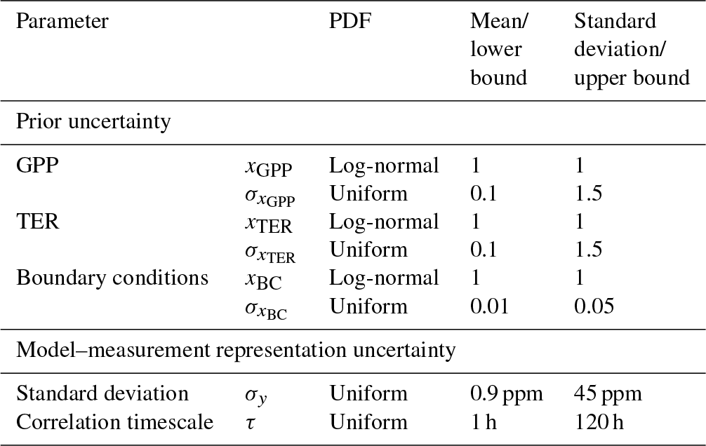
where θ is a set of hyper-parameters describing the uncertainty on x (σ_x), the model–measurement error (σ_y) and the correlation timescale in the model–measurement covariance matrix (τ). These hyper-parameters are summarised in Table 3 along with the prior PDFs used to describe them in this inversion set-up.

Table 3 Probability density functions (PDFs) for parameter and hyper-parameter scaling factors. Mean and standard deviation in the fourth and fifth columns relate to log-normal PDFs; lower bound and upper bound relate to uniform PDFs.

In this study, we have adapted the trans-dimensional method to keep a fixed set of regional basis functions (described in Sect. 2.4.3) but allow the inversions to have a variable time rather than space dimension. We perform our inversion calculations over 1 month at a time, but with the trans-dimensional case in time we find multiple scaling factors for each fixed region over the course of the inversion, down to a minimum daily resolution. Therefore, in this case k in Eq. (4) is more specifically the unknown number of time periods resolved in the inversion, which is important because CO₂ fluxes vary strongly in time and have high uncertainty in their temporal variation.

In general, there is no analytical solution to our hierarchical Bayesian equation, so we approximate the posterior solution using a reversible jump Metropolis–Hastings MCMC algorithm (Metropolis et al., 1953; Green, 1995; Tarantola, 2005; Lunt et al., 2016). The algorithm explores the possible values for each parameter by making a new proposal for a parameter value at each step of a chain of possible values. Proposals are accepted or rejected based on a comparison between the current and proposed state's fit to the data (likelihood ratio), deviation from the prior PDF (prior ratio) and a term governing the probability of generating the proposed state versus the reverse proposal (proposal ratio). More favourable parameter values or model states are always accepted; however, less favourable parameter values or model states can be randomly accepted in order to fully explore the full posterior PDF. The algorithm had a burn-in period of 5×10⁴ iterations and was then run for an additional 2×10⁵ iterations to appropriately explore the posterior distribution. At the end of the algorithm a chain of all accepted parameter values is stored (if a proposal is rejected the chain will spend longer at the previously accepted value). A histogram of this chain describes a posterior PDF for each parameter so that statistics such as the mean, median and standard deviation can be calculated. The trace of each chain was examined qualitatively to ensure that the algorithm had been run for a sufficient number of iterations to converge on a result.

2.4.2 Basis functions

Our domain is split into five spatial regions separating west-central Europe from north-east, south-east, south-west and north-west regions, shown in Fig. S1. Within the west-central Europe area (the hatched region in Fig. S1), a map of the fraction of different plant functional types in each grid cell has been used to further break down the region (Fig. S6). This is the same PFT map used in the JULES biospheric simulation (see Sect. 2.3.2). A scaling factor is solved in the inversion, scaling GPP and TER within the four outer regions and within maps of five or six PFTs in the subdomain: broadleaf tree; needleleaf tree; C₃ grasses; C₄ grasses; shrubland; and, in the case of TER, bare soil. Therefore there are 19 spatial basis functions in total.

2.4.3 Definition of Jacobian matrix

Footprints from NAME, prior fluxes, boundary conditions and basis functions are all combined into a matrix of partial derivatives, alternatively described as a “Jacobian” or “sensitivity” matrix, that describes the change in mole fraction with respect to a change in each of the input parameters. This is the “model” in the inversion set-up, denoted H in the description of the linear forward model (Eq. 7), where ε is the mismatch between modelled observations and what has actually been measured in the atmosphere. H has dimensions m (number of data points) by n (number of parameters).

$$\begin{array}{}\text{(5)}& {\displaystyle }{\displaystyle }\mathit{y}=\mathbf{H}\mathit{x}+\mathit{\epsilon }\end{array}$$

To create this linear model, we multiplied the footprints by the prior GPP and TER fluxes separately and then multiplied these by the fractional map of basis functions (described in Sect. 2.4.2) and summed over the domain. The boundary conditions were broken down by four further basis functions for each edge of the domain as explained in Sect. 2.2.2. The parameters vector, x, consisted of a set of scaling factors that multiplied the fluxes or boundary conditions. Multiplying the sensitivity matrix by the prior estimate of x, a vector of ones, yields the prior modelled mole fraction time series at a site. Therefore, during our inversion, we are updating this vector of ones as a scaling factor, to scale up or down emissions for each PFT and biospheric component to better agree with the data. Whilst in theory we have posterior information about the gross GPP and TER biospheric components separately, we combine this into a net ecosystem exchange (NEE) flux estimate, as we believe this to be more robust (Tolk et al., 2011). Therefore, throughout this paper we discuss posterior NEE estimates; however, the results of the separate sources can be found in the supplement in Figs. S7–S9.

3 Results

We have applied our CO₂ inversion set-up to UK biospheric CO₂ flux estimation using output from two different models of biospheric flux as a prior constraint in two inversions. We first describe differences between the output from the two prior models and then present the UK flux estimates found with this method, along with the spatial distribution of posterior fluxes.

3.1 Differences between DALEC and JULES

The CO₂ fluxes from DALEC and JULES differ both temporally and spatially. Figure 2a–c shows UK fluxes of GPP, TER and NEE from the two models. Most notable differences are seen in TER where JULES has a large diurnal range, whereas DALEC has a small diurnal range. Averaged to monthly resolution, the fluxes are relatively similar although DALEC has a higher TER flux from July to October. Diurnal ranges for GPP are more similar in magnitude; however, JULES exhibits a stronger sink in spring with maximum uptake in June. DALEC has maximum uptake in July and exhibits a stronger sink in autumn. Combining these two fluxes, we can see that the profile of NEE for both models is quite different. The daily maximum source from JULES remains relatively constant throughout the year, whereas the daily maximum source in DALEC follows a similar seasonal cycle to the daily maximum sink (albeit with a smaller magnitude). Monthly net fluxes are similar between both models for much of the year although JULES has stronger uptake between March and June.

In order to understand some of these seasonal differences it is useful to compare the processes taking place in each model. Section 2.3.1 and 2.3.2 provide detailed descriptions of each model and we give an overview of the main differences here. DALEC explicitly simulates the soil and litter stocks, growth and turnover processes. LAI is estimated by DALEC at a weekly time step; DALEC was calibrated using MODIS LAI estimates at the correct time and location of the analysis, explained in Sect. 2.3.1. In the JULES system, soil and litter carbon stocks are fixed values for each grid cell, calibrated from 1990 to 2000, and a fixed climatology of MODIS LAI and canopy height is used. Therefore, DALEC has interannual variability in LAI and soil carbon stocks and can adjust the parameters to find the most likely estimates in combination with other data, whereas these parameters remain constant in JULES. This is potentially advantageous for DALEC, although the use of a climatology in JULES means that noise in the MODIS LAI estimates will be averaged out. Since LAI and soil and litter carbon stocks are fixed in JULES, variability in TER and GPP fluxes is governed by meteorology – primarily temperature but also significant signals from photosynthetically active radiation and precipitation via the soil moisture. Meteorology drives the JULES model at a 2-hourly time step as opposed to a weekly time step in DALEC. Therefore, in the 2-hourly DALEC product used here, the diurnal range is not explicitly simulated and is the result of a downscaling process from a weekly resolution. This downscaling is done based on light and temperature curves as explained in Sect. 2.3.1. In DALEC, the autotrophic respiration is parameterised as a fixed fraction of the GPP for a given site but varies between sites, roughly ranging from 0.3 to 0.7. In JULES, the autotrophic respiration is the sum of plant maintenance and growth respiration terms, which are calculated separately as process-based functions of the GPP, the maximum rate of carboxylation and leaf nitrogen content (Clark et al., 2011). Typically, the autotrophic respiration in JULES is roughly 0.1–0.25 of the GPP. Therefore, there are some large differences between the model structures and parameterisations, particularly in how the respiration fluxes are simulated. This could be leading to too small a diurnal range in DALEC TER and too large a diurnal range in JULES TER.

Figures 3 and 4 show spatial maps of GPP, TER and NEE from both models averaged over winter (December, January, February) and summer (June, July, August) months. The pattern of TER is similar for both models; however, JULES always has a stronger source over Northern Ireland and DALEC has a stronger source in east England. In winter there are only small spatial variations in DALEC GPP fluxes, whereas JULES has its largest uptake in south-west England and Wales. In summer, the models are roughly in agreement in the size of the sink in Wales and the majority of England; however, JULES has a stronger sink in Scotland and Northern Ireland and DALEC has a stronger sink in central and south-east England. The differences between the models in GPP and TER lead to fairly different winter NEE flux maps. DALEC is a net source everywhere in winter, with areas of strongest net source in southern Scotland as well as east and central England. JULES is a small net winter sink in Northern Ireland, Wales, and south and central England. Summer NEE fluxes are similar between the models, although JULES has a stronger net sink in Scotland and Northern Ireland.

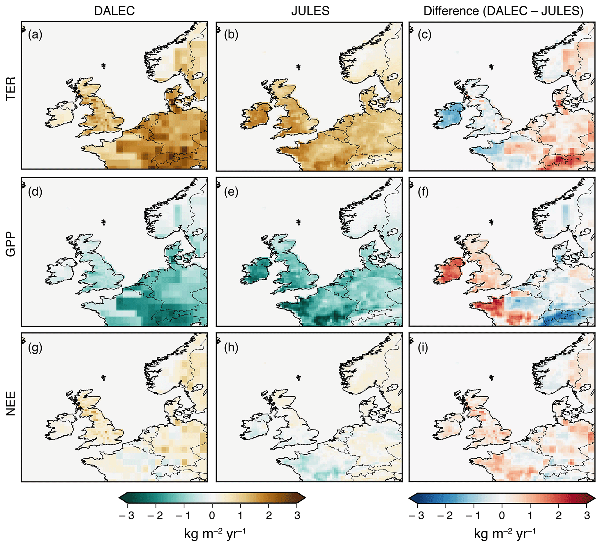
Figure 3 Average prior flux maps for winter 2013 (December 2013, January–February 2014). (a) TER from DALEC; (b) TER from JULES; (c) the difference between DALEC and JULES TER; (d) GPP from DALEC; (e) GPP from JULES; (f) the difference between DALEC and JULES GPP; (g) NEE from DALEC; (h) NEE from JULES; (i) the difference between DALEC and JULES NEE.

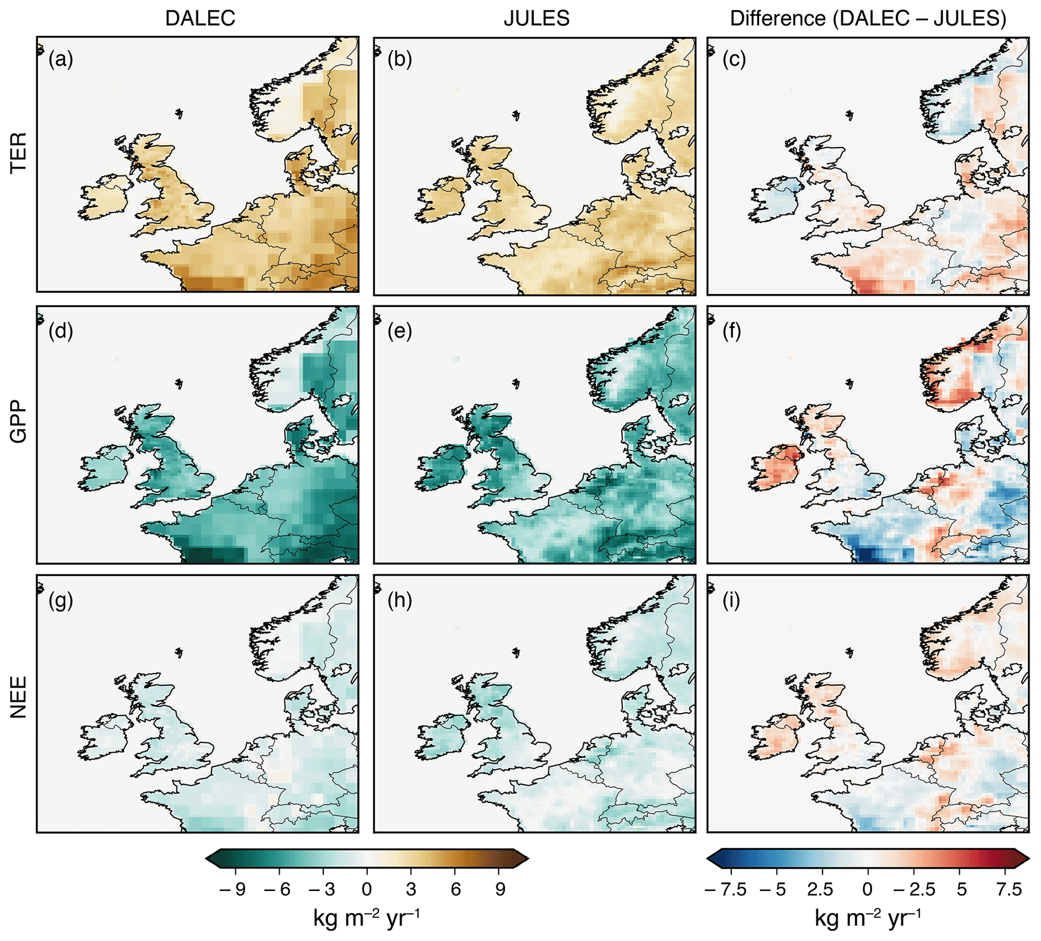
Figure 4 Prior average flux maps for summer 2014 (June–August 2014). (a) TER from DALEC; (b) TER from JULES; (c) the difference between DALEC and JULES TER; (d) GPP from DALEC; (e) GPP from JULES; (f) the difference between DALEC and JULES GPP; (g) NEE from DALEC; (h) NEE from JULES; (i) the difference between DALEC and JULES NEE.

3.2 Posterior net UK biospheric CO₂ flux 2013–2014

We have derived estimates for annual NEE from the UK using CO₂ flux output from the two different models of biospheric flux as prior information (Fig. 5 – orange and blue bars for DALEC and JULES respectively): $\mathrm{13}{\pm }_{\mathrm{87}}^{\mathrm{90}}$ Tg CO₂ yr⁻¹ (DALEC prior) and $\mathrm{76}{\pm }_{\mathrm{90}}^{\mathrm{91}}$ Tg CO₂ yr⁻¹ (JULES prior) in 2013 and $\mathrm{2}{\pm }_{\mathrm{68}}^{\mathrm{70}}$ Tg CO₂ yr⁻¹ (DALEC prior) and $\mathrm{51}{\pm }_{\mathrm{78}}^{\mathrm{80}}$ Tg CO₂ yr⁻¹ (JULES prior) in 2014. These annual net flux estimates from both models agree within the estimated uncertainties, and mean values are higher than their respective priors in both cases. The uncertainties straddle the zero net flux line, implying that the UK is roughly in balance between sources and sinks of biospheric CO₂. However, according to the inversion using JULES, a net biospheric source is less likely than in the inversion using DALEC. When added to the anthropogenic and ocean fluxes that remained fixed during the inversion, we produce the following estimates for annual total net CO₂ release from the UK (Fig. 5 – yellow and green bars for DALEC and JULES respectively): $\mathrm{448}{\pm }_{\mathrm{87}}^{\mathrm{90}}$ Tg CO₂ yr⁻¹ (DALEC prior) and $\mathrm{386}{\pm }_{\mathrm{90}}^{\mathrm{91}}$ Tg CO₂ yr⁻¹ (JULES prior) in 2013 and $\mathrm{418}{\pm }_{\mathrm{68}}^{\mathrm{70}}$ Tg CO₂ yr⁻¹ (DALEC prior) and $\mathrm{369}{\pm }_{\mathrm{78}}^{\mathrm{80}}$ Tg CO₂ yr⁻¹ (JULES prior) in 2014. While we are assuming that anthropogenic and ocean fluxes are perfectly known, the uncertainties on these fluxes are comparatively small (Peylin et al., 2011). When the anthropogenic source was varied by ±10 %, a conservatively large estimate of these uncertainties, we found posterior biospheric flux estimates using the DALEC prior that still suggest a balanced biosphere and posterior flux estimates using the JULES prior that suggest a small net sink at the lowest end of the possibilities explored here (see Fig. S10). All mean annual posterior estimates, regardless of the anthropogenic source used, suggest the prior net biospheric flux is underestimated; i.e. posterior biospheric uptake of CO₂ is smaller than predicted by the models. However, this is less statistically significant with the 2013 inversion using the DALEC prior.

The monthly posterior UK estimates using both models (Fig. 5) mostly agree well with each other within the uncertainties; however, they are both notably different from the prior estimates, especially in 2014. The posterior total UK flux estimate, achieved by adding the posterior NEE fluxes to anthropogenic and coastal ocean fluxes, shows that, according to the DALEC inversion, the UK may not be a net sink of CO₂ at any time of year in 2013 and 2014. However, the JULES inversion suggests the UK is a net sink of CO₂ in June of both years.

Figure 5 Posterior monthly net UK CO₂ flux (positive is emission to atmosphere). Orange and blue monthly fluxes are posterior net biospheric (NEE) fluxes for DALEC and JULES respectively. Prior biosphere fluxes from DALEC and JULES are shown in dashed orange and blue lines respectively. The fixed anthropogenic and ocean fluxes are denoted by the dark grey dashed line. Yellow and green monthly fluxes are the sum of the posterior NEE fluxes and the fixed anthropogenic and ocean fluxes. Shading represents 5th–95th percentile. The bar charts represent annual net UK CO₂ flux for 2013 (left) and 2014 (right). Hashed bars denote prior annual fluxes; solid bars denote posterior annual fluxes. The bar colours correspond to the line colours: left-hand bars for each model are NEE fluxes; right-hand bars for each model are total fluxes (NEE + fixed sources). Uncertainty bars represent 5th–95th percentile. DA – DALEC. JU – JULES.

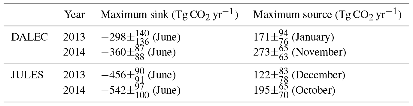
Posterior seasonal cycle amplitudes are generally smaller than the prior amplitudes, except in the DALEC inversion in 2014. Table 4 gives the posterior maximum and minimum values of NEE, leading to seasonal cycle amplitudes of 469 and 578 Tg CO₂ yr⁻¹ for 2013 and 633 and 737 Tg CO₂ yr⁻¹ for 2014, for the DALEC and JULES inversions respectively. These values are 90 % and 76 % of the prior amplitudes in 2013 and 123 % and 85 % of the prior amplitudes in 2014.

Table 4 Posterior UK estimates for the maximum net biospheric source and sink (values also shown in Fig. 5). The month in brackets indicates the month in which the maximum source or sink occurred.

The largest differences between the prior and posterior are seen in spring and summer for both models. Posterior UK NEE estimates from the DALEC inversion are in agreement with the prior for 11 months: during the first half of 2013, in the majority of winter months (December, January, February) and in June 2014. When the DALEC inversion posterior UK NEE estimates are not in agreement with the prior, they are usually larger, with a maximum difference in 2013 of $\mathrm{235}{\pm }_{\mathrm{91}}^{\mathrm{92}}$ Tg  CO₂ yr⁻¹ in August and a maximum difference in 2014 of $\mathrm{551}{\pm }_{\mathrm{84}}^{\mathrm{80}}$ Tg CO₂ yr⁻¹ in July, although in spring (March, April, May) 2014 they tend to be smaller than the prior, with a maximum difference of $-\mathrm{194}{\pm }_{\mathrm{60}}^{\mathrm{64}}$ Tg CO₂ yr⁻¹ in April. Posterior UK NEE from the JULES inversion agrees with the prior for 9 months during the 2-year period, the majority of which is between November and February. Otherwise, the posterior estimate from the JULES inversion is larger than the prior, with a maximum difference in 2013 of $\mathrm{318}{\pm }_{\mathrm{71}}^{\mathrm{70}}$ Tg CO₂ yr⁻¹ in April and a maximum difference in 2014 of $\mathrm{407}{\pm }_{\mathrm{72}}^{\mathrm{76}}$ Tg CO₂ yr⁻¹ in July.

Looking at the spring and summer differences more closely, we find that the JULES model has a systematically lower net spring flux than the posterior, and the DALEC model is either in agreement with or higher than the posterior estimate of the net spring flux. Generally, the models underestimate the net summer flux compared to the posterior flux (to the greatest extent in 2014), although the summer estimate from the JULES inversion in 2013 is not statistically different from the prior. The average spring difference between the posterior and the prior for the DALEC inversion is $-\mathrm{2}{\pm }_{\mathrm{88}}^{\mathrm{89}}$ Tg CO₂ yr⁻¹ in 2013 and $-\mathrm{133}{\pm }_{\mathrm{63}}^{\mathrm{67}}$ Tg CO₂ yr⁻¹ in 2014, whereas for the JULES inversion it is 219±87 Tg CO₂ yr⁻¹ in 2013 and $\mathrm{164}{\pm }_{\mathrm{65}}^{\mathrm{67}}$ Tg CO₂ yr⁻¹ in 2014. The average summer difference for the DALEC inversion is $\mathrm{135}{\pm }_{\mathrm{108}}^{\mathrm{111}}$ Tg CO₂ yr⁻¹ in 2013 and $\mathrm{263}{\pm }_{\mathrm{83}}^{\mathrm{82}}$ TgCO₂ yr⁻¹ in 2014, whereas for the JULES inversion it is $\mathrm{94}{\pm }_{\mathrm{107}}^{\mathrm{104}}$ Tg CO₂ yr⁻¹ in 2013 and 312±85 Tg CO₂ yr⁻¹ in 2014. The prior sink in June as estimated by the JULES model is nearly twice that of DALEC and posterior estimates tend to agree with the DALEC prior in this month.

Figure S9c shows the daily minimum and maximum in the posterior net biospheric estimates for 2014. It is worth bearing in mind at this point that while the temporal resolution of the inversion is flexible, it can go down to a minimum resolution of 1 day (as explained in Sect. 2.4.1). Therefore, the diurnal profile of TER and GPP for each model is imposed; however, it can be scaled up or down from day to day. Figure S11 shows that the inversion typically scaled the fluxes within 4 or 5 temporal regions per month, although for some parameters in some months scaling factors were found up to roughly a daily resolution. For both inversions, the posterior NEE flux shown in Fig. S9c has a similar profile. Compared to Fig. 2c the inversion tends to a seasonal cycle in daily maximum uptake that resembles that of the JULES model prior, with a turning point in maximum uptake occurring abruptly between June and July, a steep gradient in spring and a shallow gradient in autumn. On the other hand, the seasonal cycle in daily maximum source resembles that of the DALEC model prior, which has a stronger seasonal variation compared to that of the JULES model prior, albeit with a larger amplitude. This would suggest that the underestimation in net spring flux seen in the JULES prior is generally due to the model underestimating the spring source rather than overestimating the spring sink. It also suggests that the overestimation in net summer flux in the DALEC prior is possibly a combination of the model overestimating the summer sink and underestimating the summer source. The overestimation in the net summer flux in JULES is more likely to be due to an underestimation of the summer source. However, as diurnal fluxes vary on a scale nearly an order of magnitude larger than that of the monthly fluxes, it is clear that any relatively small changes in the maximum source or sink will have a relatively large effect on the daily net flux. Therefore, the monthly net flux is the more robust result here and we are not able to confidently draw conclusions from the sub-monthly results.

3.3 Posterior spatial distribution of biospheric fluxes

Figure 6 shows mean posterior net biospheric fluxes (NEE) for winter 2013 and summer 2014 from both the DALEC and JULES inversions. In winter 2013, posterior NEE fluxes from the DALEC inversion are fairly heterogeneous and are largest over south-west Scotland and east and central England. This posterior spatial distribution is roughly similar to the prior. From the inversion using JULES prior fluxes, the posterior net biospheric flux is much smoother than it is for the inversion using DALEC. It is largest in north-west England and almost zero in east England. The whole of south and central England, Wales, and Northern Ireland have increased posterior winter fluxes compared to the prior, turning these areas from a net sink in the prior to a net source in the posterior.

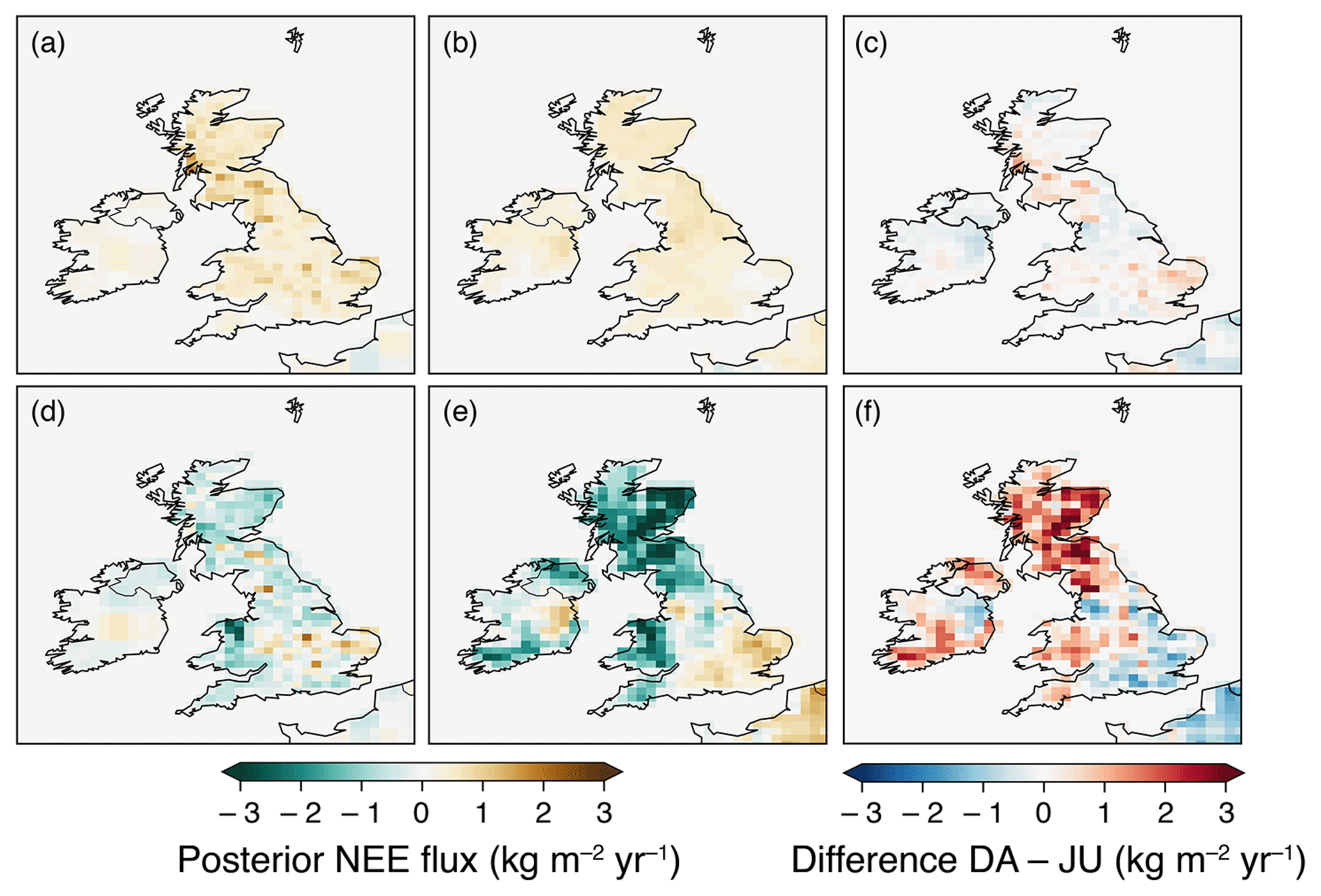
Figure 6 Posterior net biospheric (NEE) flux maps averaged over winter 2013 (December 2013, January–February 2014) and summer 2014 (June–August 2014). (a) Winter NEE flux from DALEC inversion. (b)  Winter NEE flux from JULES inversion. (c) Difference between winter NEE flux from DALEC (DA) and JULES (JU) inversions. (d) Summer NEE flux from DALEC inversion. (e) Summer NEE flux from JULES inversion. (f) Difference between summer NEE flux from DALEC (DA) and JULES (JU) inversions.

In summer 2014, NEE fluxes from the two inversions display many similarities, with areas of net source in east, central (extending further south in the JULES inversion), and north-west England and areas of net sink elsewhere. However, the net sink in the JULES inversion is larger than the DALEC inversion in Scotland, south Wales, Northern Ireland and south-west England. This differs from the prior flux maps, which have only very small areas of small net uptake in central England in DALEC and in east England in JULES. Both the DALEC and JULES posterior fluxes generally display reduced uptake compared to the prior, except in north Wales.

3.4 Model–data comparison

Agreement between the data and the posterior simulated mole fractions at the measurement sites used to constrain the inversion is greatly improved compared to prior simulated mole fractions, with R² values increasing by a minimum of 0.24 and up to 0.5 (to give values ranging between 0.53 and 0.71) and root mean square error (RMSE) decreasing by at least 1.35 ppm and up to 2.6 ppm (to give values ranging between 1.26 and 2.71 ppm). Table 5 shows all statistics for the prior and posterior mole fractions compared to the observations of atmospheric CO₂ concentrations. Overall, the fits are relatively similar between the DALEC and JULES inversions, implying that the two inversions perform similarly well by these metrics. In terms of R², the best fit to the data is observed at Heathfield in the DALEC inversion and Angus in the JULES inversion. In terms of RMSE, the best fit to the data is observed at Angus in the DALEC inversion and Mace Head in the JULES inversion. The smallest posterior mean bias is observed at Angus in the DALEC inversion and Ridge Hill in the JULES inversion. Therefore, there are some small spatial differences in how well each of the inversions is able to fit the data but no clear indication of which areas of posterior flux might be subject to the largest improvement in either inversion. Figures S12 and S13 show the residual mole fractions in 2014 and indicate that residuals are somewhat larger during the summer than the winter.

Table 5 Prior and posterior fit to data statistics for the inversion period 2013–2014. R² and RMSE are calculated monthly and averaged over this period. Values in brackets are the posterior fit statistics for the corresponding net flux inversions. ^* Weybourne data (from February to December 2013) were used for validation of the results only and were not included in the inversions.

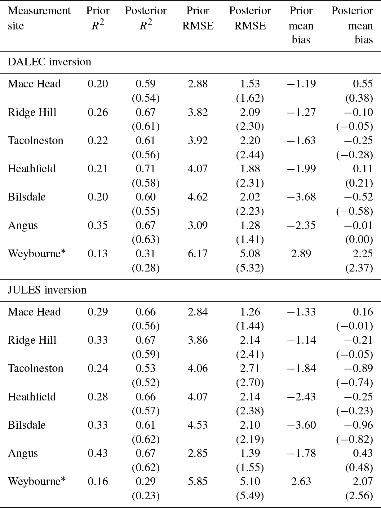
To test our posterior results against data that have not been included in the inversion, the posterior fluxes have been used to simulate mole fractions at Weybourne Atmospheric Observatory (see Fig. 1 for location in relation to the other sites and Table 1 for site information). The statistics of fit to the data are given in italics in Table 5 and show an improvement in R² of 0.18 with the DALEC inversion and 0.13 with the JULES inversion, an improvement in RMSE of 1.09 ppm with the DALEC inversion and 0.75 ppm with the JULES inversion, and an improvement in the mean bias of 0.64 ppm in the DALEC inversion and 0.56 in the JULES inversion. These results show that the a posteriori fluxes improve the fit to the data at a measurement station not included in the inversion. The results are very similar between the two inversions at this site but suggest that the DALEC inversion may perform slightly better, at least in this region of the UK. Figure S14 shows the residual mole fractions at Weybourne for each of the inversions carried out in this work.

4 Discussion

4.1 Inversion performance

Solving for both TER and GPP separately allows the JULES prior and DALEC prior inversions to converge to a similar posterior solution. Using two very different prior NEE flux estimates, we produce two similar posterior NEE flux estimates that have a similar seasonal amplitude and agree on the majority of monthly and all annual fluxes within the estimated uncertainties. This indicates that our posterior estimates are driven by the data rather than determined by the prior. However, when we carry out the same inversion but scale NEE (Fig. S15) we find the two posterior flux estimates do not converge on a common result. The posterior seasonal cycles remain relatively unchanged compared to the prior and annual net biospheric flux estimates tend to be similar to, or larger than, the prior. These annual net biospheric flux estimates are therefore 3–39 times smaller than the inversion that separates GPP and TER, meaning the posterior estimates from the two types of inversions do not overlap, even within estimated uncertainties. Evaluating the statistics of how well the NEE inversions fit the data (Table 5), we find they do not perform as well as the separate GPP and TER inversion, both at the sites included in the inversion and at the validation site, WAO. However, this is to be expected to some degree, because separating the two sources gives the inversion more degrees of freedom to fit the data.

As recommended by Tolk et al. (2011), we are only hoping to achieve an improved estimate for the net fluxes here rather than the gross GPP and TER fluxes themselves. The posterior gross fluxes are included in the supplement (Figs. S7–S9), but due to the correlation between the spatial and temporal distribution of GPP and TER they have not been presented in the main text. This can be seen in summer and winter flux maps (Figs. S7 and S8) and in the posterior annual flux estimates in Fig. S9d, in particular where JULES TER and GPP show similarly large differences from the prior. This could also be a result of the imposed diurnal cycle, as it would appear the posterior TER flux in the JULES inversion is tending to a higher daily minimum, matching that of the DALEC prior, and may ultimately be trying to move towards a smaller diurnal variation in TER. However, because the whole diurnal cycle must be scaled, the daily maximum TER must also increase and may mean the GPP must increase, causing increased uptake, to compensate for the increased source from TER. Allowing flexibility on sub-daily timescales may lead to similar estimates of GPP and TER between the two inversions with different priors. However, questions remain over whether there is enough temporal information for this to be the case.

The fact that common monthly and annual posterior net biospheric flux estimates are reached when the prior biospheric fluxes are spatially and temporally different would suggest that the choice of prior is not necessarily a major factor in guiding the inversion result for our network, when GPP and TER are scaled separately. In this respect, it is also particularly encouraging that the seasonal cycles in the posterior diurnal range are similar for both inversions (Fig. S9c).

4.2 Differences between prior and posterior NEE estimates

The posterior seasonal cycle in both inversions differs significantly from the prior. This implies that the biospheric models used to obtain prior GPP and TER fluxes are either over- or underestimating the strength of some processes, or they are omitting some processes altogether. The largest differences between the posterior solution and the prior model output are seen in spring and summer. In Sect. 3.2 we have shown that spring differences arise from an overestimation of the net spring uptake of CO₂ in the JULES model and an underestimation of the net spring uptake in the DALEC model in 2014. However, in summer (particularly in 2014), the posterior net UK fluxes are higher than both priors in July and August.

One process that occurs during the months July and August is crop harvest. Harvest is not directly resolved in either of the models of the biosphere used in this work, thereby providing a possible explanation for the differences between the posterior and prior in these months. Harvest typically occurs between July and September and arable agricultural land covered 26 % of the UK in 2013 and 2014 (DEFRA, 2014, 2015), so there is potential for unaccounted activity in this area to cause large changes to net CO₂ fluxes. The areas of net source in summer (shown in Fig. 6) do also coincide with areas of large-scale agriculture (e.g. east and central England). Crop harvest potentially changes the biosphere in the following ways: firstly, crops mature en masse, leading to an abrupt loss of productivity. Secondly, during harvest there is an abrupt removal of biomass and input of harvest residues on the field. This increases litter input that is readily available for decomposition, increasing heterotrophic respiration. Thirdly, when the field is ploughed the soil is disturbed, which can increase heterotrophic respiration. Finally, when the crop is no longer covering the soil surface this layer can become drier and the energy balance is altered. In Smallman et al. (2014), the reduction in atmospheric CO₂ concentration due to crop uptake is reported for 2006 to 2008 and an abrupt increase in atmospheric CO₂ can be seen between June (peak source) and August, where CO₂ uptake from crops is halted as a result of harvest. Harvest may explain the abrupt shift from net sink to net zero or net source observed between July and August in DALEC in 2013 and June and July in both models in 2014. The earlier time in 2014 does coincide with a year of early harvest (DEFRA, 2015) although this may well be fortuitous. Later in the summer, there may be some plant regrowth in ploughed fields leading to increased GPP. This would be consistent with the shallower gradient observed in net biospheric fluxes between September and October 2013 in the DALEC posterior estimate, between August and September 2014 in the JULES posterior estimate, and the decrease in net flux observed between July and September 2014 in the DALEC posterior estimate.

If agricultural activity is the source of the July, August and September difference between prior and posterior UK NEE estimates, then it could amount to emissions of 4 %–10 % of currently reported annual anthropogenic emissions in 2013 and 17 %–19 % in 2014. However, other explanations for this difference could be large uncertainties in the seasonal disaggregation of anthropogenic fluxes, uncertainties in the transport model, or a combination of over- and underestimation of other biospheric processes.

4.3 Implications for UK CO₂ emissions estimates

The results of UK biospheric CO₂ fluxes using our set-up suggest the UK biosphere is roughly in balance, whereas prior estimates from models of the biosphere estimate a net sink. Even when we assume an uncertainty on our anthropogenic fluxes of 10 % (a conservative estimate), inversions using both models still give mean posterior estimates that are larger than their respective priors (see Fig. S10). Therefore, when using models of the biosphere to contribute to inventory estimates of CO₂ emissions, care must be taken to attribute sufficient uncertainties to model estimates, otherwise the amount of CO₂ taken up by the biosphere on an annual basis may be overestimated. Methods such as the one described in this paper could provide an important constraint on the UK's biospheric CO₂ fluxes as carbon sequestration processes, such as reforestation, and other land use change activities are increasingly used as policy solutions to contribute to carbon targets.

5 Conclusion

We have developed a framework for estimating net biospheric CO₂ fluxes in the UK that takes advantage of recent innovation in atmospheric inverse modelling and a relatively dense regional network of measurement sites. Two inversions are carried out using prior flux estimates from two different models of the biosphere, DALEC and JULES. Fluxes of GPP and TER are scaled separately in the inversions. Despite significant differences in prior biospheric fluxes, we find consistent monthly and annual posterior flux estimates, suggesting that in this study the choice of model to provide biospheric CO₂ flux priors in the inversion is not a major factor in guiding the inversion result with our framework and network. However, given the hypothesised importance of missing process representation from both models, e.g. agriculture, an improved model may result in an improved analysis, reducing uncertainties and biases highlighted in this study.

Similarly to Tolk et al. (2011), we find that the NEE is more robustly derived if GPP and TER are solved separately and then combined a posteriori. Our results suggest that inversions that scale only NEE could be underestimating net CO₂ fluxes, as we find posterior estimates 3–39 times smaller than those obtained using an inversion where GPP and TER are separated.

We find that the UK biosphere is roughly in balance, with annual net fluxes (averaged over the study period) of 8±79 and 64±85 Tg CO₂ yr⁻¹ according to the DALEC and JULES inversions respectively. These mean annual fluxes are systematically higher than their respective priors, implying that net biospheric fluxes are underestimated in the models of the biosphere used in this study. The posterior seasonal cycles from both inversions differ significantly from the prior seasonal cycles and generally have a reduced amplitude of 90 % and 76 % of the prior amplitude in 2013 according to the DALEC and JULES inversions respectively as well as 85 % of the prior amplitude in 2014 according to the JULES inversion; however, the posterior seasonal cycle amplitude from the DALEC inversion in 2014 was increased by 122 %. Our results suggest an overestimated net spring flux in the JULES model and an overestimation of the net summer flux in both models of the biosphere. We propose that the difference seen between the prior and posterior flux estimates in summer and early autumn could be a result of the disturbance caused by crop harvest, leading to an abrupt reduction in plant CO₂ uptake and increase in respiration sources, as it is not taken into account in either model. However, this hypothesis is just one of a combination of uncertain factors that could lead to the differences seen, so further work would be needed to investigate the importance of crop harvest in UK CO₂ emissions.

The method developed and described here represents a first step towards looking at the UK biospheric CO₂ budget with a hierarchical Bayesian trans-dimensional MCMC inverse modelling framework. Further work is required to robustly constrain biospheric CO₂ fluxes through comparison with other model set-ups.