Emissions of methane in Europe inferred by total column measurements

Using five long-running ground-based atmospheric observatories in Europe, we demonstrate the utility of long-term, stationary, ground-based measurements of atmospheric total columns for verifying annual methane emission inventories. Our results indicate that the methane emissions for the region in Europe between Orléans, Bremen, Białystok, and Garmisch-Partenkirchen are overestimated by the state-of-the-art inventories of the Emissions Database for Global Atmospheric Research (EDGAR) v4.2 FT2010 and the high-resolution emissions database developed by the Netherlands Organisation for Applied Scientific Research (TNO) as part of the Monitoring Atmospheric Composition and Climate project (TNO-MACC_III), possibly due to the disaggregation of emissions onto a spatial grid. Uncertainties in the carbon monoxide inventories used to compute the methane emissions contribute to the discrepancy between our inferred emissions and those from the inventories.

1 Introduction

Recent global policy agreements have led to renewed efforts to reduce greenhouse gas emissions to cap global temperature rise (e.g., Conference of the Parties 21, COP 21; UNFCCC, 2015; Kona et al., 2016). This, in turn, has motivated countries to seek methods of reducing their greenhouse gas emissions. In Europe, methane emissions account for a significant fraction (about 11 % by mass of CO₂ equivalent) of the total greenhouse gas emissions (UNFCCC, 2017). The lifetime of atmospheric methane is significantly shorter than for carbon dioxide, its 100-year global warming potential is significantly larger, and it is at near steady state in the atmosphere; therefore, significant reductions in methane emissions are an effective short-term strategy for reducing greenhouse gas emissions (Dlugokencky et al., 2011). Emission reduction strategies that include both methane emission reductions and carbon dioxide reductions are thought to be among the most effective at slowing the increase in global temperatures (Shoemaker et al., 2013). Thus, it is important to know exactly how much methane is being emitted and the geographic and temporal source of the emissions. This requires an approach that combines state-of-the-art emissions inventories that contain information about the specific point and area sources of the known emissions and timely and long-term measurements of greenhouse gases in the atmosphere to verify that the emissions reduction targets are met.

Because atmospheric methane is well-mixed and has a lifetime of about 12 years (Stocker et al., 2013), it is transported far from its emission source, making source attribution efforts challenging from atmospheric measurements alone. Atmospheric measurements are often assimilated into “flux inversion” models to locate the sources of the emissions (e.g., Houweling et al., 2014) but rely on model wind fields to drive transport, and they also tend to have spatial resolutions that do not resolve subregional scales. Methane measurement schemes that constrain emissions on local and regional scales are thus important to help identify the sources of the emissions and to verify inventory analyses. Regional- or national-scale emissions are important to public policy as those emissions are reported annually to the United Nations Framework Convention on Climate Change (UNFCCC).

The atmospheric measurement techniques that are used to estimate methane emissions include measurements made in situ, either on the ground, from tall towers, or from aircraft. Remote sensing techniques are also used, either from space or from the ground. The spatial scale of the sensitivity to emissions differs with the measurement technique: surface in situ measurements provide information about local emissions on urban scales (e.g., McKain et al., 2015; Hopkins et al., 2016), and aircraft in situ measurements can provide information about regional- and synoptic-scale fluxes (e.g., Jacob et al., 2003; Kort et al., 2008, 2010; Wofsy, 2011; Baker et al., 2012; Frankenberg et al., 2016; Karion et al., 2016). Satellite remote sensing techniques provide information useful for extracting emission information on larger scales (regional to global) (e.g., Silva et al., 2013; Schneising et al., 2014; Alexe et al., 2015; Turner et al., 2015) and for large point or urban sources (e.g., Kort et al., 2012, 2014; Nassar et al., 2017). Several studies have shown the importance of simultaneous measurements of co-emitted species (e.g., C₂H₆ and CH₄ or CO and CO₂, Aydin et al., 2011; Simpson et al., 2012; Peischl et al., 2013; Silva et al., 2013; Hausmann et al., 2016; Wunch et al., 2016; Jeong et al., 2017) or co-located measurements (e.g., Wunch et al., 2009, 2016), showing the added analytical power of the combination of atmospheric tracer information. Ground-based remote sensing instruments have been used to estimate methane emissions on urban (e.g., Wunch et al., 2009; Hase et al., 2015; Wunch et al., 2016) and sub-urban (e.g., Chen et al., 2016; Viatte et al., 2017) scales. In Hase et al. (2015), Viatte et al. (2017), and Chen et al. (2016), the authors have placed mobile ground-based remote sensing instruments around a particular emitter of interest (e.g., a city, dairy, or neighborhood) and have designed short-term campaigns to measure the difference between upwind and downwind atmospheric methane abundances. From these differences the authors have computed emission fluxes. However, there is a network of nonmobile ground-based remote sensing instruments that have been collecting long-term measurements of atmospheric greenhouse gas abundances. These instruments were not placed intentionally around an emitter of interest, but collectively they ought to contain information about nearby emissions. To date, there have been no studies that have attempted to extract regional methane emission information from these existing ground-based remote sensing observatories.

In this paper, we will describe our methods for computing the emissions of methane using five stationary ground-based remote sensing instruments located in Europe in Sect. 2. Our results and comparisons to the state-of-the-art inventories are shown in Sect. 3, and we summarize our results in Sect. 4.

2 Methods

Our study area is the region between five long-running atmospheric observatories situated in Europe. Three of the stations are in Germany: Bremen (Notholt et al., 2014), Karlsruhe (Hase et al., 2014), and Garmisch-Partenkirchen (Sussmann and Rettinger, 2014). The other two are in Poland (Białystok, Deutscher et al., 2017) and France (Orléans, Warneke et al., 2014). Each station measures the vertical column-averaged dry-air mole fraction of carbon dioxide (${\mathrm{X}}_{{\mathrm{CO}}_{\mathrm{2}}}$), carbon monoxide (X_CO), methane (${\mathrm{X}}_{{\mathrm{CH}}_{\mathrm{4}}}$), and other trace gas species. The locations are shown in Fig. 1, overlaid on a nighttime light image from the National Aeronautics and Space Administration (NASA) to provide a sense of the population density of the area. These observatories are part of the Total Carbon Column Observing Network (TCCON, Wunch et al., 2011) and have been tied to the World Meteorological Organization trace-gas scale through comparisons with vertically integrated, calibrated in situ profiles over the observatories (Wunch et al., 2010, 2015; Messerschmidt et al., 2011; Geibel et al., 2012).

Figure 1 The locations of the TCCON observatories overlaid on a NASA nighttime light image. From west to east, the stations are Orléans (or, pink), Karlsruhe (ka, green), Bremen (br, blue-green), Garmisch-Partenkirchen (gm, orange), and Białystok (bi, purple).

Following a similar method to Wunch et al. (2009, 2016), we estimate emissions of methane from the data recorded from the TCCON observatories, coupled with gridded inventories of carbon monoxide within the region. We compute changes (or “anomalies”) in ${\mathrm{X}}_{{\mathrm{CH}}_{\mathrm{4}}}$ and X_CO that we will refer to as $\mathrm{\Delta }{\mathrm{X}}_{{\mathrm{CH}}_{\mathrm{4}}}$ and ΔX_CO, and we then compute the slopes relating $\mathrm{\Delta }{\mathrm{X}}_{{\mathrm{CH}}_{\mathrm{4}}}$ to ΔX_CO. From the computed slopes (α), we can infer emissions of methane (E${}_{{\mathrm{CH}}_{\mathrm{4}}}$) if emissions of carbon monoxide (E_CO, in mass per unit time) are known, using the following relationship:

$$\begin{array}{}\text{(1)}& {\mathrm{E}}_{{\mathrm{CH}}_{\mathrm{4}}}=\mathit{\alpha }{\displaystyle \frac{m_{{\mathrm{CH}}_{\mathrm{4}}}}{m_{\mathrm{CO}}}}{\mathrm{E}}_{\mathrm{CO}},\end{array}$$

where $\frac{m_{{\mathrm{CH}}_{\mathrm{4}}}}{m_{\mathrm{CO}}}$ is the ratio of the molecular masses of CH₄ and CO.

In Wunch et al. (2009, 2016), measurements from a single atmospheric observatory were used to infer emissions because the unique dynamics of the region advected the polluted air mass into and out of the study area diurnally. In this paper, we rely on several stations to provide measurements of the boundary of the study region to measure CO and CH₄ emitted between the stations. This analysis relies on a few assumptions about the nature of the emissions. First, that the lifetimes of the gases of interest are longer than the transport time within the region. This is the case both for methane, which has an atmospheric lifetime of 12 years, and for carbon monoxide, which has an atmospheric lifetime of a few weeks. Second, we assume that typical emissions are consistent over time periods longer than a few days so that they are advected together. The nature of the emissions in this region (mostly residential and industrial energy needs) supports this assumption. Third, we assume that the spatial distribution of the emissions is similar for CH₄ and CO, as confirmed by the inventory maps (Fig. A3). This method does not require carbon monoxide and methane to be co-emitted (as they generally do not have the same emissions sources).

To compute anomalies and slopes, we first filter the data to minimize the impact of data sparsity and air mass differences between stations (Appendix Appendix A). Then, for each station, the daily median value is subtracted from each measurement. This reduces the impact of the station altitude and any background seasonal cycle from aliasing into the results. Subsequently, we compute the differences in the ${\mathrm{X}}_{{\mathrm{CH}}_{\mathrm{4}}}$ and X_CO abundances measured at the same solar zenith and solar azimuth angles on the same day at two TCCON stations. By computing anomalies at the same solar zenith angles, we minimize any impact that air-mass-dependent biases could have on the calculated anomalies. This analysis is repeated for all combinations of pairs of stations within the study area. The vertical sensitivity of the TCCON measurements is explicitly taken into account by dividing the anomalies by the surface layer column averaging kernel value, as we assume that the anomalies are due to emissions near the surface. The slopes computed for each year and each pair of stations are shown in Fig. 2.

The farthest distance between the European TCCON stations included in this study is between Orléans and Białystok (1580 km). Climatological annual mean surface wind speeds from the National Centers for Environmental Prediction (NCEP) and National Center for Atmospheric Research (NCAR) reanalysis (Kalnay et al., 1996) within the study area are about 6 km h⁻¹ (Fig. A1). The air from Orléans will quickly mix vertically from the surface where the winds aloft are more rapid than at the surface (see Appendix Appendix B). Thus, air from Orléans would normally reach Białystok in a few days. To determine whether these anomalies are consistent throughout the transport time through the study area, we compute anomalies between sites lagged by up to 14 days. The slopes of the anomalies do not change significantly or systematically with the lag time (Appendix Appendix B; Fig. A2), presumably because the atmospheric composition within the study area is relatively well-mixed or because the emissions are relatively consistent from day to day within the study area.

Figure 2 The bars show the methane to carbon monoxide anomaly slopes for each site pair. The method of computing these anomaly slopes is detailed in Sect. 2 of the main text. The black targets indicate the median value of the slope for that year, when all site pairs are considered simultaneously, and the 25th and 75th quartiles of the median value are indicated by the vertical black bars. Outliers are indicated by open black circles.

Previous papers have used carbon dioxide instead of carbon monoxide to infer methane emissions. We choose to compute emissions using measurements of X_CO instead of ${\mathrm{X}}_{{\mathrm{CO}}_{\mathrm{2}}}$ in this work because the natural CO₂ fluxes in the region are large compared with the anthropogenic emissions, and they have a strong diurnal and seasonal cycle. The distance between the stations is large enough that local (sub-daily) uptake of CO₂ differs from station to station, significantly obscuring the relationships between methane and carbon dioxide, and thus the anomaly slopes, especially in the summer months. While the emissions inventory of anthropogenic CO₂ may be more accurate than the CO inventory in the region, the presence of these large natural fluxes of CO₂ precludes its use in the anomaly slope calculation. The accuracy of our method, therefore, is limited by the accuracy of the carbon monoxide emission inventory. Fires could provide a large flux of CO without a large CH₄ flux, and this should also be taken into consideration in these types of analyses. In our study area fluxes from fires are small.

2.1 Inventories

To obtain an estimate of carbon monoxide emissions (E_CO) within the study area, we use gridded inventories and sum the emissions within the study area to compare with our emissions inferred from the TCCON measurements (see Appendix Appendix C and Fig. A3 for details). The two inventories employed here are the Emissions Database for Global Atmospheric Research (EDGAR) and the Netherlands Organisation for Applied Scientific Research (TNO) high-resolution emissions database developed as part of the Monitoring Atmospheric Composition and Climate project (TNO-MACC_III). The EDGAR version v4.3.1_v2 of January 2016 annual gridded inventory is available at $\mathrm{0.1}{}^{\circ }\times \mathrm{0.1}{}^{\circ }$ spatial resolution and reports global emissions from the year 2000 to 2010 (Olivier et al., 1994; EC-JRC and PBL, 2016). The TNO-MACC_III inventory is a Europe-specific air quality emissions inventory, available on a $\mathrm{0.125}{}^{\circ }\times \mathrm{0.0625}{}^{\circ }$ grid, and reports emissions for 2000–2011 (Kuenen et al., 2014). Both EDGAR and TNO-MACC_III provide spatially and temporally coincident methane inventories which we use to compare with our inferred emissions. We use the EDGAR version v4.2 FT2010 and the TNO-MACC_III methane inventories.

Using country-level emissions reported through 2015 from the European Environment Agency (EEA, 2015), we extrapolate the EDGAR and TNO-MACC_III gridded inventory CO emissions for the study area through 2015. This facilitates more direct comparisons with the TCCON measurements, which begin with sufficient data for our study in 2009. We extrapolate the emissions by scaling the total emissions from the countries that are intersected by the area of interest (Germany, Poland, Belgium, France, Luxembourg, and the Czech Republic) to the last reported year of emissions from the inventory. We then assume that the same scaling factor applies for each subsequent year. The details of the extrapolation method are in Appendix Appendix D and Figs. A4 and A5.

The time series of the reported emissions from 2000 to 2015 are shown in Fig. 3. The inventories and scaled country-level reported emissions for this region suggest that emissions of CO and CH₄ have decreased by about 40 % and 20 %, respectively, between 2000 and 2015. The TNO-MACC_III carbon monoxide emissions are on average 15 % higher than the EDGAR v.4.3.1 emissions in the study area. The total TNO-MACC_III and EDGAR methane emissions agree to within 2 % in the study area.

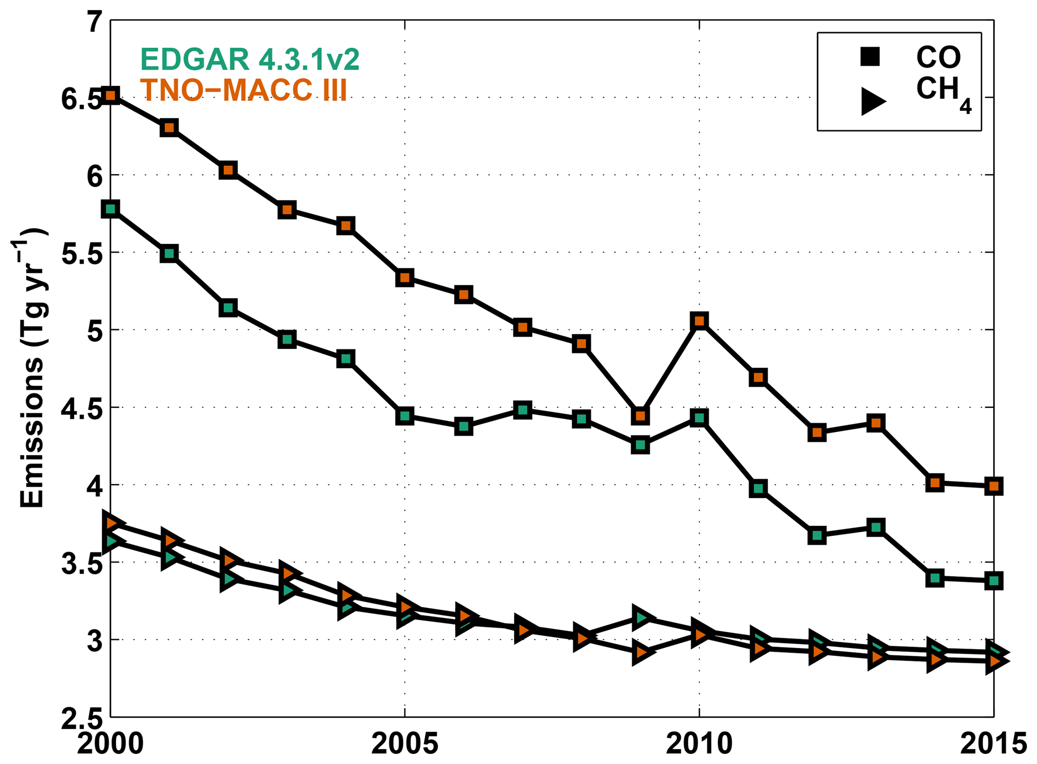
Figure 3 This figure shows the summed EDGAR (green) and TNO-MACC_III (orange) emissions within the study area for CO (squares) and CH₄ (triangles). The study area is defined in Fig. 1. All emissions are shown in units of Tg yr⁻¹. Extrapolation begins after 2010 for EDGAR and 2011 for TNO-MACC_III.

An earlier version of the EDGAR carbon monoxide inventory was evaluated by Stavrakou and Müller (2006) and Fortems-Cheiney et al. (2009), who assimilated satellite measurements of CO using the EDGAR v3.3FT2000 CO emissions inventory as the a priori. Stavrakou and Müller (2006) found that, over Europe, the a posteriori emissions increase by less than 15 % when assimilating carbon monoxide from the Measurements of Pollution in the Troposphere (MOPITT) satellite instrument (Emmons et al., 2004). Fortems-Cheiney et al. (2009) assimilated Infrared Atmospheric Sounding Interferometer (IASI) CO (Clerbaux et al., 2009) and MOPITT CO and found that the a posteriori emissions increase by 16 % and 45 %, respectively.

The more recent EDGAR v4.3.1 CO emissions in our study are 24 % lower than the EDGAR v3.3FT2000 CO emissions for the year 2000, so it may be that the EDGAR v4.3.1 CO emissions are significantly underestimated. However, assimilations of CO are known to be very sensitive to the chemistry described in the model: most notably the OH chemistry (Protonotariou et al., 2010; Yin et al., 2015). Therefore, it is difficult to determine how much of the discrepancy between versions of the model is from the inventory or the model chemistry.

The EDGAR methane inventory has been evaluated in several previous studies. It has been shown to overestimate regional CH₄ emissions (e.g., Wunch et al., 2009; Wecht et al., 2014) but to underestimate oil and gas emissions (e.g., Miller et al., 2013; Buchwitz et al., 2017). However, recent methane isotope analysis by Röckmann et al. (2016) has suggested that the EDGAR inventory overestimates fossil-fuel-related emissions. The study area of interest here has little oil and gas production, except for some test sites in Poland (USEIA, 2015), no commercial shale gas industry, and few pipelines.

2.2 Model experiment

To test whether the anomaly method described in Sect. 2 can accurately infer methane emissions, we conducted a modeling experiment using version v12.1.0 of the GEOS-Chem model (http://www.geos-chem.org, last access: 4 January 2019) to simulate methane and carbon monoxide for the year 2010. The model is driven by the Modern-Era Retrospective analysis for Research and Applications, version 2 (MERRA-2) meteorology from the NASA Global Modeling and Assimilation Office. The native resolution of the meteorological fields is $\mathrm{0.25}{}^{\circ }\times \mathrm{0.3125}{}^{\circ }$, with 72 vertical levels from the surface to 0.01 hPa, which we degraded to $\mathrm{2}{}^{\circ }\times \mathrm{2.5}{}^{\circ }$ and 47 vertical levels. We use the linear CO-only and CH₄-only simulations of GEOS-Chem, with prescribed monthly mean OH fields. In the CO-only simulation, global anthropogenic emissions are from EDGAR v4.3.1, which are overwritten regionally with the following emissions: the Cooperative Programme for Monitoring and Evaluation of the Long-range Transmission of Air Pollutants in Europe (EMEP), the U.S. Environmental Protection Agency National Emission Inventory for 2011 (NEI2011), the MIX inventory for Asia, the Visibility Observational (BRAVO) Study Emissions Inventory for Mexico, and the criteria air contaminants (CAC) inventory for Canada. The sources of CO from the oxidation of CH₄ and volatile organic compounds (VOCs) are prescribed following Fisher et al. (2017). For the CH₄-only simulation, the emissions are as described in Maasakkers et al. (2019). Global anthropogenic emissions are from EDGAR v4.3.2, but the US emissions were replaced with those from Maasakkers et al. (2016), and emissions from wetlands are from WetCHARTs version 1.0 (Bloom et al., 2017). For both CO and CH₄ simulations, emissions from biomass burning are from the Quick Fire Emissions Dataset (QFED) (Darmenov and Silva, 2015). The biomass burning in the study area produces less than 2 % of the total anthropogenic emissions of CO.

Figure 4 This figure compares seasonally averaged modeled total X_CO with the X_CO contribution from emissions in Europe. Each season has two maps: the left map shows the total X_CO and the right map shows the contribution from European emissions (X_CO−Eur). The spatial pattern of the gradients in modeled X_CO between the TCCON stations is reflected in the European contribution.

We used identical OH fields (from version v7-02-03 of GEOS-Chem) for the CO and CH₄ simulations, so that the chemical losses of methane and carbon monoxide are consistent, and ran tagged CO experiments so that we could identify the source of the emissions. The model atmospheric carbon monoxide and methane profiles were integrated to compute simulated X_CO and ${\mathrm{X}}_{{\mathrm{CH}}_{\mathrm{4}}}$. To illustrate the sensitivity of the modeled fields to European emissions, we show the seasonal means of the modeled X_CO sampled at the five TCCON stations in Fig. 4. Also plotted is the column contribution (X_CO−Eur) from CO emissions only in Europe (defined as the broader region between 0–45^∘ E and 45–55^∘ N). As can be seen, the spatial pattern of the differences in modeled X_CO between the TCCON stations is reflected in X_CO−Eur. We calculated the anomalies in X_CO and X_CO−Eur, using the same approach employed with the atmospheric data, and found that the anomalies in X_CO−Eur, which represent the direct influence of European emissions on atmospheric CO, account for about 35 % of the anomalies in X_CO. This confirms that the X_CO anomalies between the TCCON stations are sensitive to European emissions.

Figure 5 This figure shows the results from the modeling experiment using GEOS-Chem. Panel (a) shows the model $\mathrm{\Delta }{\mathrm{X}}_{{\mathrm{CH}}_{\mathrm{4}}}$–ΔX_CO slopes for each month and pair of stations (indicated by the colors). The median slopes for each month are overlaid with grey squares. Panel (b) shows the model carbon monoxide emissions (excluding VOC and methane oxidation) and the model methane emissions. The inferred methane emissions from our tracer–tracer slope method are plotted in pink squares. Panel (c) shows the annual methane emissions from the tracer–tracer slope method and the model.

To estimate the modeled CH₄ emissions using the modeled CO, the modeled X_CO and ${\mathrm{X}}_{{\mathrm{CH}}_{\mathrm{4}}}$ were interpolated to the locations of the TCCON stations and anomalies and slopes were computed. We then applied Eq. (1) to our anomaly slopes to compute methane emissions from the known CO emissions, accounting for only the CO emissions from anthropogenic, biomass burning, and biofuel sources. We neglect sources of CO emissions from the oxidation of CH₄ and VOCs because the column enhancements for those emissions are relatively spatially uniform across this region of Europe, and thus they should not contribute significantly to the anomalies. The resulting annual CH₄ emissions agree well with the model emissions: the inferred emissions from the anomaly analysis are higher than the model emissions by less than 2 % (Fig. 5).

While the inferred annual emissions agree well with the modeled annual emissions, the seasonal pattern of the emissions inferred from the anomaly analysis differs from that of the model. The anomaly analysis overestimates emissions in the winter and underestimates emissions in the summer. This may be due to small spatial inhomogeneities in the column enhancements from VOC (biogenic) emissions that influence the anomaly analysis most in summertime when VOC emissions are largest. Including the VOC emissions in the total carbon monoxide emissions leads us to infer annual methane emissions that are overestimated by 15 %, increasing the inferred summertime emissions without significantly changing the inferred wintertime emissions.

The seasonal analysis suggests that the 2 % agreement in the annual emission estimate may reflect the compensating effects of discrepancies over the seasonal cycle, and improving the seasonal estimate may require a better treatment of the VOC contribution to atmospheric CO. Nevertheless, the results here suggest that for this region of Europe, where VOC and methane oxidation emissions lead to relatively spatially uniform column enhancements and fire emissions are small, we can successfully use the anomaly method described in Sect. 2 to infer annual methane emissions.

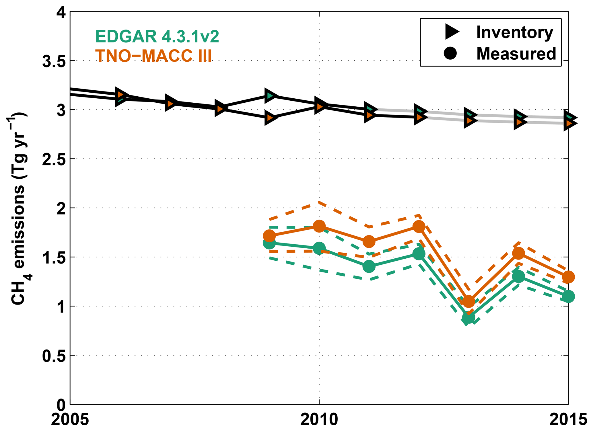
Figure 6 The black line is the summed EDGAR (green) and TNO-MACC_III (orange) methane emissions within the study area shown in Fig. 1. The grey lines indicate the projected emissions based on scaling the country-level emissions reported by the UNFCCC (UNFCCC, 2017) to the area emissions in 2010 for EDGAR and 2011 for TNO-MACC_III. The lower solid lines show the emissions inferred from the TCCON anomaly analysis using CO emissions from the two models, and the dashed lines indicate the 5th and 95th percentiles.

3 Results and discussion

To compute methane emissions, we apply Eq. (1) to our anomaly slopes and the inventory-reported carbon monoxide emissions in the study region (Fig. 6). If we choose the mean of the reported CO emissions from EDGAR v4.3.1 and TNO-MACC_III, the methane emissions we compute within the study area based on the TCCON measurements are 1.7±0.3 Tg yr⁻¹ in 2009, with a non-monotonic decrease to 1.2±0.3 Tg yr⁻¹ in 2015. The uncertainties quoted here are from the standard errors on the data slope fitting only; we have not included uncertainties from the inventories. The magnitude of methane emissions we compute from the TCCON data are, on average, about 2.3 times lower than the methane emissions reported by EDGAR and about 2 times lower than the methane emissions reported by TNO-MACC_III.

Our method of inferring methane emissions depends critically on the carbon monoxide inventory. The carbon monoxide emissions for 2010 in the study area from our GEOS-Chem model run, derived from EMEP emissions, were 6.4 Tg, about 35 % higher than the average of the EDGAR and TNO-MACC_III emissions for that year. This magnitude underestimate has also been suggested by Stavrakou and Müller (2006) and Fortems-Cheiney et al. (2009) using independent data. Using the GEOS-Chem carbon monoxide emissions increases the methane emissions inferred by the anomaly analysis to 2.4±0.3 Tg in 2010. This value remains lower than the EDGAR and TNO-MACC_III methane emissions estimates for 2010, which are 3 Tg, but by only 20 %. Therefore, we find that the inventories likely overestimate methane emissions, but the accuracy of our results relies on the accuracy of the carbon monoxide inventory.

Although the EDGAR and TNO-MACC_III inventories agree to within 15 % in carbon monoxide emissions and 2 % in methane emissions in the study region, they spatially distribute these emissions differently. Maps of the spatial differences between the TNO-MACC_III and EDGAR emissions are shown in Fig. 7 for carbon monoxide and Fig. 8 for methane. EDGAR estimates larger emissions of carbon monoxide from the main cities in the study region and the surrounding areas. This is clearly visible from the difference map (Fig. 7), where cities such as Hamburg, Berlin, Prague, Wrocław, Warsaw, Munich, Paris, and Vienna appear in blue. However, the overall carbon monoxide emissions from TNO-MACC_III in the study area are higher than EDGAR, and this comes from regions between the main cities, particularly in Poland and eastern France.

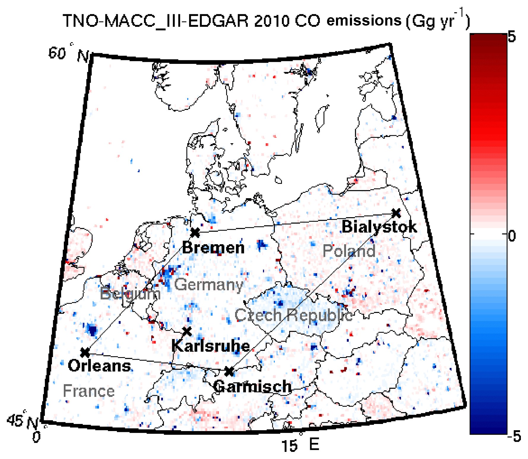
Figure 7 This map shows the difference between the TNO-MACC_III carbon monoxide emissions and the EDGAR emissions for the year 2010. The black straight lines delineate the study area from the surrounding region. The TCCON stations included in this study are marked with black “x” symbols and labeled in black bold font. The countries intersected by or contained within the study area are labeled in grey. Warm (red) colors indicate that the TNO-MACC_III inventory is larger than the EDGAR inventory; cool (blue) colors indicate that the EDGAR inventory is larger than TNO-MACC_III.

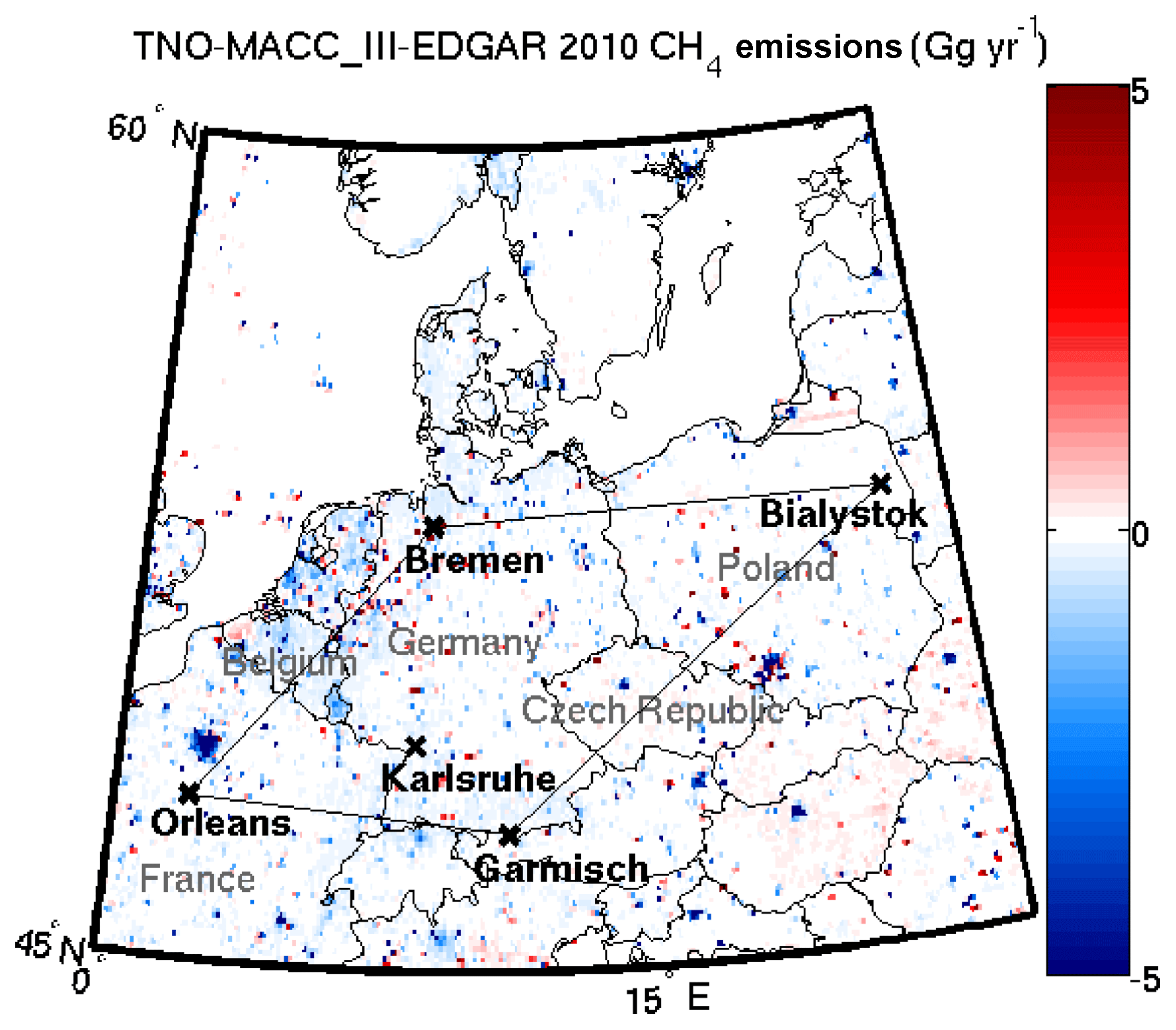
Figure 8 This map shows the difference between the TNO-MACC_III methane emissions and the EDGAR emissions for the year 2010. The labeling and coloring follows that in Fig. 7.

The differences between EDGAR and TNO-MACC_III methane emissions also show that the EDGAR emissions estimates near large cities are significantly larger (Fig. 8). In contrast to the carbon monoxide spatial distribution, the TNO-MACC_III methane emissions are generally smaller everywhere, except for discrete point sources.

Comparing country-level carbon monoxide emissions reported in 2010 with the inventories shows reasonable agreement, which is expected since the inventories use country-level reports as input. The sum of the carbon monoxide emissions within the entire countries of Germany, Poland, France, Luxembourg, Belgium, and the Czech Republic differ between EDGAR and TNO-MACC_III by 18 %, with EDGAR estimates lower than those from TNO-MACC_III. Emissions from Germany, most of which are included in the study area, differ by only 6 % between EDGAR and TNO-MACC_III, again with EDGAR estimates lower than TNO-MACC_III. The national carbon monoxide emissions reported to the Convention on Long-range Transboundary Air Pollution (LRTAP Convention, https://www.eea.europa.eu/ds_resolveuid/0156b7a0ca47485593e7754c52c24afd, last access: 15 November 2017,  EEA, 2015) agree to within a few percent of the TNO-MACC_III country-level emissions (e.g., 5.5 % for Germany in 2010).

The differences between 2010 country-level emissions estimates are larger for methane: EDGAR estimates are larger than TNO-MACC_III estimates by 36 % when summing all countries intersected by the study area and 8 % when considering only German emissions. The TNO-MACC_III country-level emissions estimates agree to within a few percent of the UNFCCC (http://di.unfccc.int/time_series, last access: 15 November 2017) country-level reported methane emissions (e.g., 8 % for Germany in 2010).

The differences between the EDGAR and TNO-MACC_III inventories suggest that the spatial distribution of emissions is less certain than the larger-scale emissions, since the total carbon monoxide and methane emissions between the inventories agree to within 15 % and 2 %, respectively, in the study area, but these estimates can disagree by a factor of 2 on city-level scales.

If we assume that the national-scale methane emissions are correctly reported in EDGAR and TNO-MACC_III, our results indicate that the methane emissions in the region are incorrectly spatially distributed in the inventories. It could be that point or urban sources outside the study area but within the countries intersected by the study area emit a larger proportion of the country-level emissions than previously thought.

4 Conclusions

Using co-located measurements of methane and carbon monoxide from five long-running ground-based atmospheric observing stations, we have shown that in the area of Europe between Orléans, Bremen, Białystok, and Garmisch-Partenkirchen, the inventories likely overestimate methane emissions and point to a large uncertainty in the spatial distribution (i.e., the spatial disaggregation) of country-level emissions. However, the magnitude of our inferred methane emissions relies heavily on the EDGAR v4.3.1 and TNO-MACC_III carbon monoxide inventories, and thus there is a need for rigorous validation of the carbon monoxide inventories.

This study demonstrates the potential of clusters of long-term ground-based stations monitoring total columns of atmospheric greenhouse and tracer gases. It also shows the potential of having co-located measurements of multiple pollutants to derive better estimates of emissions. These types of observing systems can help policy makers verify that greenhouse gas emissions are reducing at a rate necessary to meet regulatory obligations. The atmospheric measurements are agnostic to the source (and country of origin) of the methane, measuring only what is emitted into the atmosphere in a given area. Thus, they can help validate and reveal inadequacies in the current inventories, and, in particular, how country-wide emission reports are disaggregated on a grid. To enhance these results, simultaneous measurements of complementary atmospheric trace gases, such as ethane, acetylene, nitrous oxide, nitrogen dioxide, ammonia, and isotopes, would help distinguish between sources of methane. This would provide additional valuable information that would likely improve inventory disaggregation.