the Creative Commons Attribution 4.0 License.
the Creative Commons Attribution 4.0 License.
 | 22 Mar 2019
Effects of two different biogenic emission models on modelled ozone and aerosol concentrations in Europe
Giancarlo Ciarelli
Emmanouil Oikonomakis
Imad El-Haddad
Francesco Canonaco
Colin O'Dowd
Jurgita Ovadnevaite
María Cruz Minguillón
Urs Baltensperger
André S. H. Prévôt
Biogenic volatile organic compound (BVOC) emissions are one of the essential inputs for chemical transport models (CTMs), but their estimates are associated with large uncertainties, leading to significant influence on air quality modelling. This study aims to investigate the effects of using different BVOC emission models on the performance of a CTM in simulating secondary pollutants, i.e. ozone, organic, and inorganic aerosols. European air quality was simulated for the year 2011 by the regional air quality model Comprehensive Air Quality Model with Extensions (CAMx) version 6.3, using BVOC emissions calculated by two emission models: the Paul Scherrer Institute (PSI) model and the Model of Emissions of Gases and Aerosol from Nature (MEGAN) version 2.1. Comparison of isoprene and monoterpene emissions from both models showed large differences in their general amounts, as well as their spatial distribution in both summer and winter. MEGAN produced more isoprene emissions by a factor of 3 while the PSI model generated 3 times the monoterpene emissions in summer, while there was negligible difference (∼4 %) in sesquiterpene emissions associated with the two models. Despite the large differences in isoprene emissions (i.e. 3-fold), the resulting impact in predicted summertime ozone proved to be minor (<10 %; MEGAN O3 was higher than PSI O3 by ∼7 ppb). Comparisons with measurements from the European air quality database (AirBase) indicated that PSI emissions might improve the model performance at low ozone concentrations but worsen performance at high ozone levels (>60 ppb). A much larger effect of the different BVOC emissions was found for the secondary organic aerosol (SOA) concentrations. The higher monoterpene emissions (a factor of ∼3) by the PSI model led to higher SOA by ∼110 % on average in summer, compared to MEGAN, and lead to better agreement between modelled and measured organic aerosol (OA): the mean bias between modelled and measured OA at nine measurement stations using Aerodyne aerosol chemical speciation monitors (ACSMs) or Aerodyne aerosol mass spectrometers (AMSs) was reduced by 21 %–83 % at rural or remote stations. Effects on inorganic aerosols (particulate nitrate, sulfate, and ammonia) were relatively small (<15 %).
- Article
(10128 KB) - Full-text XML
-
Supplement
(1745 KB) - BibTeX
- EndNote


Biogenic volatile organic compounds (BVOCs) from the terrestrial biosphere play an important role in atmospheric chemistry. They affect production of ozone (Calfapietra et al., 2013; Curci et al., 2009) and the formation process of secondary inorganic aerosol (SIA) (Aksoyoglu et al., 2017) and are the largest source of secondary organic aerosol (SOA) worldwide (Bonn et al., 2004; Hallquist et al., 2009; Hodzic et al., 2016; Kirkby et al., 2016). Emissions of BVOCs such as isoprene, monoterpenes (MTs), and sesquiterpenes (SQTs) are now commonly used as inputs within numerous chemical transport models (CTMs). While in many model inter-comparison studies anthropogenic emissions are harmonised, biogenic emissions usually differ (Bessagnet et al., 2016; Colette et al., 2017; Im et al., 2015; Solazzo et al., 2012). Different approaches in biogenic emission models may result in substantial difference in predicted emission rates of BVOCs (Messina et al., 2016; Oderbolz et al., 2013). Although there are a few studies comparing different BVOC models (Karl et al., 2009; Keenan et al., 2009; Steinbrecher et al., 2009), comprehensive studies showing the impact of using different BVOC emission models on secondary pollutants in Europe are scarce. Some studies report the effect of biogenic emissions with zero-out simulations (Sartelet et al., 2012) or with doubled BVOC emissions (Aksoyoglu et al., 2017; Ciarelli et al., 2016). Curci et al. (2009) compared effects of two different biogenic emission inventories, one based on Guenther et al. (1995) and one based on Steinbrecher et al. (2009), on ozone in Europe for 4 years (1997, 2000, 2001, 2003). However, the limitation of ozone production might have been altered due to large emission reductions of the various precursors in Europe during the past decades. Understanding the potential influence of biogenic emissions on European air quality is therefore of great importance, especially under the continuously reduced anthropogenic emissions since the early 1990s.
BVOCs, dominated by isoprene and monoterpenes, are generated from biosynthesis of precursor isopentenyl pyrophosphate in plants (Kesselmeier and Staudt, 1999). Isoprene is emitted from leaf surfaces immediately after synthesis (referred to as synthesis emission), while monoterpenes are mostly stored in plant organs after their production (pool emission) and some monoterpene species have synthesis emissions as well. The emission processes are influenced by various factors, such as plant species, foliage biomass, temperature, solar radiation as well as carbon and water availability (Grote and Niinemets, 2008), leading to high uncertainty in the estimates of BVOC emissions. Current BVOC emission models are mostly based on an empirical bottom-up approach using emission factors as a function of leaf temperature and photosynthetically active radiation (PAR) (Andreani-Aksoyoglu and Keller, 1995; Guenther et al., 2006, 2012; Solmon et al., 2004). Although most of these models share similar algorithms, the inputs such as emission factors and land use types might vary widely for different studies. For example, the widely used MEGAN (Model of Emissions of Gases and Aerosols from Nature) (Guenther et al., 2012) estimates 19 categories of BVOC species by emission factors based on 15 CLM4 (Community Land Model) plant function types (PFTs) (e.g. broadleaf evergreen tropical tree, broadleaf deciduous temperate shrub). To account for variability of different tree species within the same PFT, MEGAN version 2.1 provides emission factors for more than 2000 ecoregions worldwide based on tree species composition and tree-species-specific emission factors (Guenther et al., 2012). For regional simulations in which more detailed land use and vegetation information were available, Solmon et al. (2004) estimated isoprene and monoterpene emissions in France based on CORINE Land Cover (CLC) land use data with a resolution of 50–100 m and BVOC emission factors of each tree species. Significant influence of land use and vegetation on the spatial distribution and magnitude of estimated BVOC emissions has been reported by many studies (Hantson et al., 2017; Oderbolz et al., 2013; Rosenkranz et al., 2015; Steinbrecher et al., 2009; Szogs et al., 2017).
As an important input to air quality models, BVOC emissions strongly influence the simulated concentrations of ozone and aerosols, with great spatial and temporal difference. BVOCs play crucial roles in both the formation and removal processes of ozone (Calfapietra et al., 2013). Comparison between MEGAN and another widely used biogenic emission model, the Biogenic Emission Inventory System (BEIS), indicated that the influence of biogenic emission models on ozone simulation results over the United States is far greater than using a different photosynthetically active radiation (PAR) input (Zhang et al., 2017). The potential influence of biogenic emissions on aerosol modelling results is more complicated. BVOCs are oxidised by reactions with oxidants like hydroxyl radicals (OH), nitrate radicals (NO3), and ozone (O3) and generate secondary organic aerosols via gas-to-particle partitioning (Griffin et al., 1999; Hoffmann et al., 1997). Different estimates of BVOC emissions directly influence the amount of biogenic SOA precursors (mainly MTs and SQTs) (Bonn et al., 2004), while they also indirectly influence the aerosol simulations via effects on oxidants (Ayres et al., 2015; Calfapietra et al., 2013; Ng et al., 2017). Significant influence of anthropogenic activities and climate conditions on biogenic SOA formation (Carlton et al., 2010; Fu et al., 2014; Hoyle et al., 2011) makes it even more challenging to understand the effect of BVOC emissions on SOA simulations. Moreover, BVOCs also influence the secondary inorganic aerosol formation by changing the oxidant concentrations (Aksoyoglu et al., 2017; Karambelas, 2013; Sotiropoulou et al., 2004; Zhang et al., 2016). Aksoyoglu et al. (2017) found that doubled BVOC emissions in Europe led to an increase in particulate inorganic nitrate concentrations by up to 35 %.
In spite of an increasing interest in understanding the influences of biogenic emissions on ozone and aerosols, limitations still remain: most of the studies focus on short periods (mostly in summer), while the potential influence of BVOCs on SOA could still be high in winter at the local scale, the evaluation of modelled OA is challenged by the scarcity of field measurements, and not much attention has been paid to the effects of BVOCs on SIA by different biogenic models. In this study, we investigated the effects of different estimates of BVOC emissions on modelled ozone and aerosol concentrations in Europe. Biogenic emissions were estimated by two BVOC emission models with different land cover inputs and emission factors: MEGAN as a widely used model globally and the PSI model to represent models developed for a specific region. The BVOC emissions from the two models were then used as input for the regional air quality model Comprehensive Air Quality Model with extensions (CAMx) to simulate gaseous and particulate pollutant concentrations in 2011. The modelled results were evaluated by comparisons with ozone measurements from the European air quality database (AirBase) and aerosol measurement from nine Aerodyne aerosol chemical speciation monitor (ACSM) or Aerodyne aerosol mass spectrometer (AMS) stations over Europe.
2.1 Regional air quality model CAMx
The regional air quality model CAMx version 6.3 (http://www.camx.com/, last access: 12 March 2019) with the VBS (volatility basis set) scheme (Koo et al., 2014) was used to simulate the year 2011 in this study. The model domain (15∘ W–35∘ E, 35∘–70∘ N) covered Europe with a horizontal resolution of . The meteorological inputs were prepared by the Weather Research and Forecasting Model Advanced Research (WRF-ARW) version 3.7.1 (NCAR, 2016; Skamarock et al., 2008). We used the ECMWF (European Centre for Medium-Range Weather Forecasts) global atmospheric reanalysis ERA-Interim data as initial and boundary conditions for the WRF model, with a spatial resolution of and a time step of 6 h (Dee et al., 2011). The meteorological fields from the WRF output were further processed by WRFCAMx version 4.4 (http://www.camx.com/download/support-software.aspx, last access: 12 March 2019) to match the CAMx vertical layers and to prepare the required parameters (e.g. vertical diffusivity). In CAMx, there were 14 terrain-following vertical layers reaching up to 460 hPa, with the first layer being ∼20 m thick. The Carbon Bond 6 Revision 2 (CB6r2) mechanism (Hildebrandt Ruiz and Yarwood, 2013) was used for the gas-phase chemistry. Aqueous sulfate and nitrate formation in resolved cloud water was simulated by the Regional Acid Deposition Model (RADM) algorithm (Chang et al., 1987). Partitioning of inorganic aerosol components between the gas and particle phases was calculated by the ISORROPIA thermodynamic model (Nenes et al., 1998). Organic aerosol formation from anthropogenic (including both land and ships) and biogenic (terrestrial) sources was modelled by the 1.5-D VBS organic aerosol chemistry and partitioning module (Koo et al., 2014), which describes the evolution of OA in the 2-D space of oxidation state and volatility. The standard CAMx v6.3 treats the aging and partitioning processes of secondary aerosols from biogenic and biomass burning sources in the same basis sets. To distinguish the contributions of biogenic and biomass burning sources to OA, we separated the combined basis set VBS–PBS (V: vapour; P: particle; S: secondary; B: biogenic and biomass burning) into two sets: VBIS–PBIS (BI: biogenic) for biogenic sources and VBBS–PBBS (B: biomass burning) for biomass burning sources.
The gridded initial concentrations of chemical species in each layer of the model domain as well as at the domain lateral boundaries were obtained from the global model data MOZART-4/GEOS-5 (Horowitz et al., 2003) with a time resolution of 6 h. The ozone column densities were obtained from Total Ozone Mapping Spectrometer (TOMS) data by the National Aeronautics and Space Administration (ftp://toms.gsfc.nasa.gov/pub/omi/data/, last access: 12 March 2019) and photolysis rates were calculated using the Tropospheric Ultraviolet and Visible (TUV) Radiation Model version 4.8 (NCAR, 2011). Anthropogenic emissions of non-methane volatile organic compounds (NMVOCs), SO2, NOx, CO, NH3, PM10, and PM2.5 were obtained from the high-resolution European emission inventory TNO-MACC (The Netherlands Organization for Applied Scientific Research - Monitoring Atmospheric Composition and Climate)-III. As an update to TNO-MACC-II (Kuenen et al., 2014), TNO-MACC-III has a major improvement in spatial distribution proxies, especially for urban areas (van Der Gon, 2015). The NMVOC speciation was conducted following the approach described by Passant (2002). The PM emissions were further split into organic carbon, elemental carbon, sodium, sulfate, and crustal minerals, based on country-specific profiles provided by TNO.
2.2 Biogenic emission models
Two different biogenic emission models were used to calculate BVOC emissions (isoprene, MT, SQT), i.e. MEGAN version 2.1 (Guenther et al., 2012) and the BVOC model developed by the Laboratory of Atmospheric Chemistry, Paul Scherrer Institute (referred to as the PSI model in this study; Andreani-Aksoyoglu and Keller, 1995). MEGAN is among the most widely used modelling systems estimating emission rates of BVOCs from terrestrial ecosystems. MEGAN version 2.1 covers 147 individual BVOC species within 19 categories (Guenther et al., 2012). The PSI model was first developed for fine-resolution estimation of monoterpene and isoprene emissions in Switzerland (Andreani-Aksoyoglu and Keller, 1995) and was later expanded to the European domain (Oderbolz et al., 2013; Oikonomakis et al., 2018). Both MEGAN and PSI models estimate biogenic emissions through an empirical bottom-up approach with similar algorithms based on standard emission rates (at a leaf temperature of 30 ∘C and photosynthetically active radiation of 1000 µmol m−2 s−1) and the emission response to environmental conditions (Guenther et al., 2012; Andreani-Aksoyoglu and Keller, 1995). The major difference between the two models is that MEGAN uses emission factors specific to PFT (plant function type), while the PSI model uses emission factors specific to plant species. Here we mainly focus on the differences in the calculation of emission rates and inputs of land use and vegetation. A general comparison between the major inputs of the PSI model and MEGAN version 2.1 is presented in Table 1.
Table 1Comparison between the major input of the PSI model and MEGAN version 2.1.
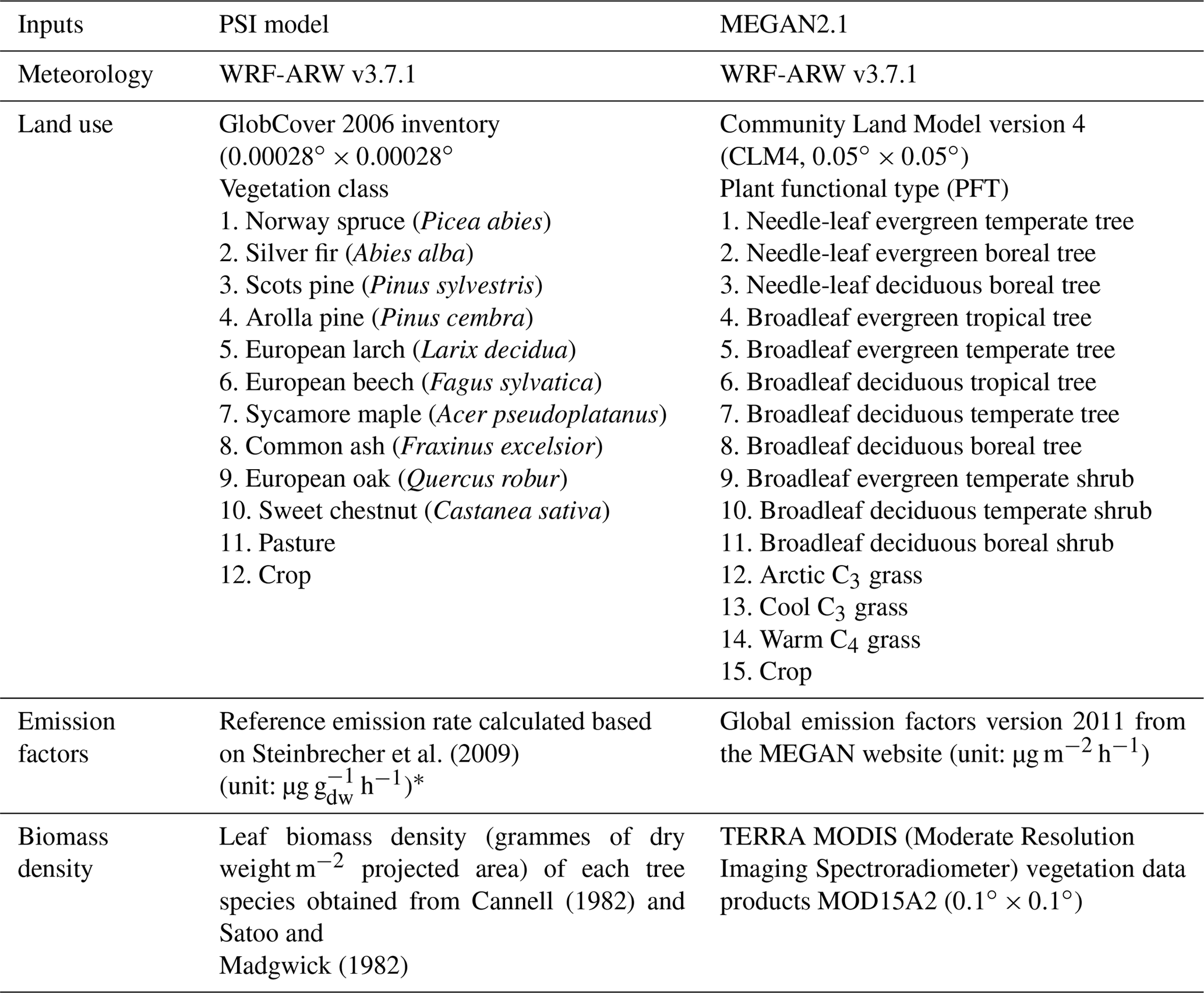
*dw in the unit means dry weight of biomass.
2.2.1 Emission rates
MEGAN estimates the reference emission rates by emission factors of 15 PFTs, as listed in Table 1. The Global Emission Factors (version 2011) from the MEGAN website (http://lar.wsu.edu/megan/guides.html, last access: 12 March 2019) were used in this study. Emission factors of compounds are given for each of the 15 PFTs (Guenther et al., 2012). Tree-species-based emission factors and forest species composition profiles for more than 2000 ecoregions worldwide were used to generate the high-resolution () global emission factor dataset. On the other hand, the PSI model uses reference emission rates of typical plant species in Europe (see Table 1). The reference emission rates (µg g(dry weight)−1 h−1) of isoprene and monoterpenes from forests, pasture, and crops were calculated based on algorithms given by Lamb et al. (1993). Isoprene emissions from Norway spruce were assumed to be about 10 % of α-pinene emission rates during daytime (Steinbrecher, 1989). SQTs are the least studied among the identified BVOCs due to their high reactivity and relatively low vapour pressure (Duhl et al., 2008). Determination of their basal emission rates is therefore challenging. In the PSI model, SQT emissions were treated only as pool emissions and assumed to be 5 % (by weight) of the monoterpene emissions based on the emission rate data for 116 species compiled from various studies as given by Steinbrecher et al. (2009).
2.2.2 Response functions
Isoprene, one of the most important BVOC species, is released after biosynthesis by volatilisation, which depends on both temperature and solar radiation. On the other hand, monoterpenes are stored in large storage pools after their production in the plant organs. Emissions of monoterpenes are mostly temperature-dependent, although there are some species that have both light- and temperature-dependent synthesis emissions of MTs (Tingey et al., 1980). In the PSI model, the isoprene emissions are corrected by light (γL) and temperature (γT) response functions based on the algorithm described by Guenther et al. (1993):
where α (=0.0027), CL1 (=1.066), CT1 (=95 000 J mol−1), CT2 (=230 000 J mol−1), and TM (=314 K) are all empirical coefficients determined by nonlinear fitting based on emission rate measurements, R is the gas constant (8.314 J K−1 mol−1), and Ts is the standard leaf temperature (303.16 K). The response functions of the isoprene emission in MEGAN are based on Guenther et al. (1999), an updated version of Guenther et al. (1993). The major difference of the improved algorithm is the inclusion of the influence of past temperature and light conditions. New empirical coefficients Topt and Eopt calculated by the average leaf temperature over the past 24 and 240 h are added to include the continuous influence over time, respectively (Eq. 3):
where . A detailed introduction to Topt and Eopt can be found in Guenther et al. (2006).
For the light-independent response of MT pool emissions, similar exponential corrections are used by MEGAN and the PSI model, which are based on Lamb et al. (1993) and Tingey et al. (1980) as shown in Eq. (4):
where E is the MT emission at temperature T, Es is the emission under standard conditions (Ts=30 ∘C), and β is the slope coefficient of dlnE dT−1. The slope value β has a wide range between 0.057 and 0.144 according to previous literature (Guenther et al., 1993). The value of 0.1 is used for most MT species (e.g. α-pinene, β-pinene, 3-carene, and limonene) in MEGAN2.1, while the values are between 0.065 and 0.077 for different MT species in the PSI model. The light-dependent synthesis emissions of MTs were considered in MEGAN2.1 as described in Guenther et al. (2012). Depending on different MT species, the light-dependent fraction of MT emissions ranges between 0.2 and 0.8 for MEGAN. In the PSI model, the light-dependent emissions from Norway spruce are calculated for each monoterpene species as a function of PAR based on the data of Schürmann (1993). In addition to the light and temperature response, MEGAN2.1 also covers some other factors such as leaf age and leaf area index (Guenther et al., 2012). Since the correction of soil moisture and CO2 dependence is not included in the offline version of MEGAN (Emmerson et al., 2016), we used the default parameterisation where the correction factors were set to 1.
The variation in light and temperature within the forest canopy are corrected by a canopy model in both the PSI model and MEGAN. The PSI model uses the canopy model by Baldocchi et al. (1985) combined with experiments in Hartheim forest (Germany) and central Switzerland (Joss, 1995). The detailed algorithm of the canopy correction for the PSI model was reported by Keller et al. (1995). The MEGAN canopy environmental model is based on Guenther et al. (1999), which estimates incident PAR and the temperature of sun and shade leaves at different canopy depths. Details can be found in Guenther et al. (2006, 2012). A BVOC reduction of about ∼20 % due to the canopy model was reported for the PSI model by Oderbolz et al. (2013). Although different canopy models could influence the modelled BVOC emission, such influence was within the uncertainty range of observed fluxes (Guenther et al., 2006; Lamb et al., 1996).
2.2.3 Inputs of driving variables
Three types of basic driving variables are required for both MEGAN and the PSI model, namely meteorological conditions, land use, and biomass density. The meteorological data provide hourly gridded information of temperature, solar radiation, wind speed, moisture, and surface pressure to drive the model simulation of emission response. We used the same meteorological data retrieved from the WRF-ARW model as input for both models. The main difference between the two model inputs is in the land use and leaf biomass density.
MEGAN2.1 uses the Community Land Model version 4 (CLM4) including 15 PFTs as shown in Table 1. In this study, we adopted for MEGAN the same global PFT map as in Sindelarova et al. (2014) with a resolution of 0.05∘. For the PSI model, the GlobCover 2006 inventory by the European Space Agency (http://due.esrin.esa.int/page_globcover.php, last access: 12 March 2019) was used. This inventory was developed based on MERIS (MEdium Resolution Imaging Spectrometer) FRS (Fine Resolution Full Swath product) level 1B data during December 2004 to June 2006 (Bicheron et al., 2008). The raw data have a fine resolution of 300 m and 64 categories of land use types, e.g. needle-leaf evergreen forest, broadleaf deciduous forest, and mixed broadleaf and needle-leaf forest. The grid-scale fractions of needle-leaf, broadleaf, and mixed forests were first calculated based on the GlobCover inventory data. The mixed forest was assumed to be composed of 50 % needle-leaf and 50 % broadleaf species. Different tree species in the same category may have different emission factors. For instance, although all belong to broadleaf tree species, oak (Quercus) has a high emission rate, while beech (Fagus sylvatica) and maple (Acer) are negligible BVOC emitters. Even within the same genus, there might be large differences in emissions, e.g. two oak species, where Quercus robur is a high isoprene emitter and Quercus suber a low isoprene emitter (Steinbrecher et al., 2009). Europe has a relatively low abundance of flora in both diversity and numbers, and six tree species cover two-thirds of the forest area, namely Scots pine, Norway spruce, beech, maritime pine, European oak, and evergreen oak (Simpson et al., 1999). Therefore, in the PSI model, we classified the forests into 10 typical forest species (see Table 1: vegetation classes 1–10) found in Europe based on the country-specific forest species profile from Simpson et al. (1999). The original 35 forest species in Simpson et al. (1999) were grouped into 10 classes (including five coniferous species and five broadleaf species), and the ratio of each species class to the total coniferous forest and broadleaf forest was calculated (Table S2). The ratio of “other trees” was proportionally added to the 10 tree species. As the other trees are mainly in a few Mediterranean countries, their influence on the whole domain is small. The species coverage was then generated by multiplying the forest coverage from GlobCover with the country-specific tree species profile.
The biomass density in MEGAN was calculated by the canopy environment module based on the satellite data of the leaf area index (LAI, m2 leaves m−2 projected area) with a time step of 8 days. The TERRA MODIS vegetation data products MOD15A2 were downloaded from the NASA Earth Observations website (https://neo.sci.gsfc.nasa.gov/view.php?datasetId=MOD15A2_E_LAI&year=2011, last access: 12 March 2019). The grid-scale LAI was then divided by the fraction of vegetation coverage of each grid (sum of PFT) to get the average LAI of vegetation-covered surfaces (LAIv).
As the reference emission rates of the PSI model are based on dry weight of leaf biomass, the leaf biomass density factors (grammes of dry weight m−2 projected area) of each tree species (Cannell, 1982; Satoo and Madgwick, 1982) were explicitly used in the PSI model. To simulate the vertical variation in foliar biomass in the canopy, the biomass density was scaled by the leaf area distribution in each canopy layer as described in Oderbolz et al. (2013). The temporal variation in the biomass was simulated by monthly factors for different plant types. For example, the PSI model assumes that the leaf biomass of deciduous trees, such as oak and larch, turn to zero in the winter months (November–March) and crops only have biomass in the growing season (April–August).
2.3 Observation datasets and statistics
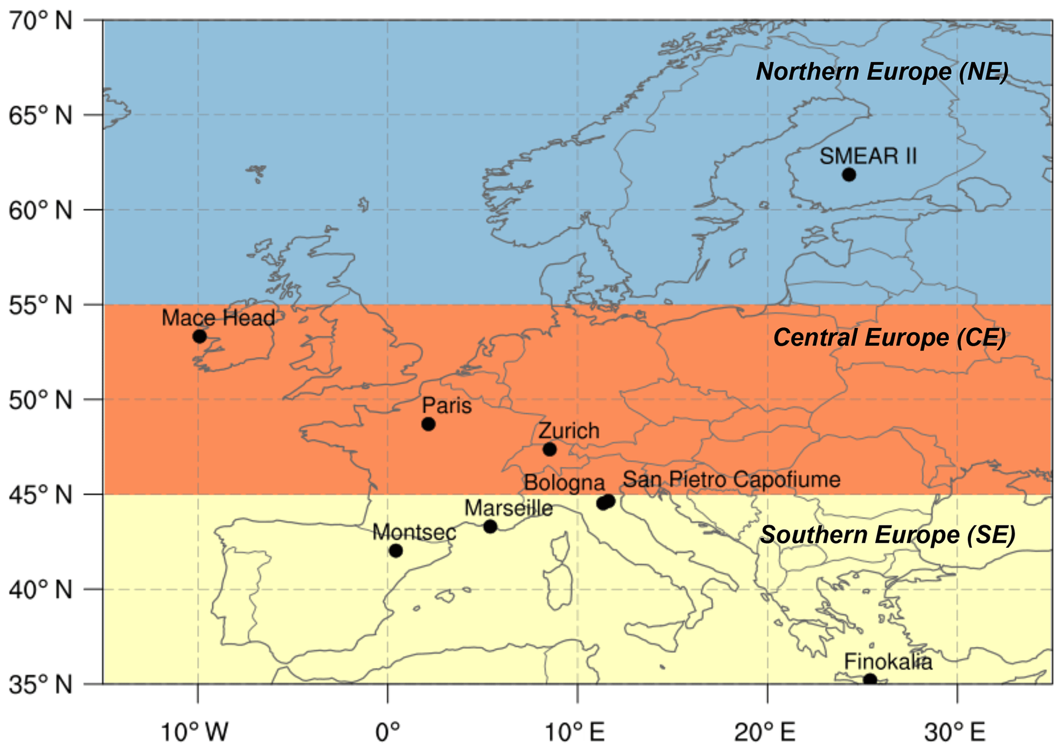
Two types of measurement datasets were used to evaluate the model results. Measurements of hourly ozone concentrations in 2011 were extracted from the European air quality database (AirBase v7) from the European Environment Agency (Mol and Leeuw, 2005). To reduce the uncertainties arising from the model resolution, only ozone measurements at background rural stations were used in the model evaluation. Concentrations of OA and secondary inorganic aerosol (particulate nitrate, sulfate, and ammonium) were obtained from ACSM/AMS measurements at nine stations: Zurich (Canonaco et al., 2013), Mace Head (Ovadnevaite et al., 2014; Schmale et al., 2017), Montsec (Ripoll et al., 2015), Bologna and San Pietro Capofiume (Gilardoni et al., 2014), Paris SIRTA (Site Instrumental de Recherche par Télédétection Atmosphérique) (Petit et al., 2015), Marseille (Bozzetti et al., 2017), Finokalia (as continuation of Hildebrandt et al., 2010), and the SMEAR II (Station for Measuring Forest Ecosystem–Aerosol Relations) Hyytiälä station (Kortelainen et al., 2017). The spatial distribution of the measurement sites is shown in Fig. 1. Zurich, Bologna, and Marseille are urban sites; Paris SIRTA is a suburban site; and Mace Head, Finokalia, San Pietro Capofiume, and Montsec are in rural or remote areas. We divided the whole domain into three regions to enable a comparison for different latitudes: northern Europe (NE: 55–70∘ N), central Europe (CE: 45–55∘ N), and southern Europe (SE: 35–45∘ N). The time span of OA observations at each station is shown in Fig. S1. The measurements cover nearly the whole year of 2011 in Zurich (except for January) and Mace Head (except for November and December), while other stations cover shorter periods (Fig. S1). The modelled concentrations at the surface (first) layer were interpolated to the location of the stations to compare with the measurements. The statistical metrics, such as mean bias (MB), mean error (ME), mean fractional bias (MFB), mean fractional error (MFE), and root-mean-square error (RMSE), were calculated and compared for two CAMx simulations using different BVOC emissions obtained by MEGAN and the PSI model. The definitions of these statistical metrics are presented in Table S1.
3.1 Biogenic VOCs in Europe
BVOC emissions estimated by the PSI model and MEGAN showed significant differences in both spatial and temporal variations. To evaluate the seasonal differences, we compared the BVOC emissions in February and July to represent winter and summer periods, respectively. BVOC emissions in winter are much lower than in summer, especially for isoprene, which is mainly emitted by deciduous broadleaf trees. The PSI model produced negligible isoprene in winter, as the leaf biomass of oak trees, the largest isoprene emitters, was set to zero during that period. For monoterpenes, which are mainly emitted by evergreen needle-leaf forests, the seasonal difference was less obvious than for isoprene, although the emissions in winter were lower than in summer due to lower temperatures (about 82 % and 96 % lower than in summer for the PSI model and for MEGAN, respectively).
Isoprene emissions by MEGAN were substantially higher than those in the PSI model (Fig. 2a) by a factor of 2.9 on average in summer. The highest difference occurred in southern Europe (Fig. S2a), where the highest grid-scale absolute difference (MEGAN−PSI) reached 203 kg cell−1 h−1 in Spain. The major reason for low isoprene emissions from the PSI model is the assumption of oak being the main broadleaf tree species emitting isoprene, while all the broadleaf trees and shrubs (PFT4–PFT11) have positive emission factors in MEGAN. On the other hand, the PSI model estimates more monoterpene emissions than MEGAN in general (Fig. 2b). The total emissions in the whole domain were 486 t h−1 (winter) and 2768 t h−1 (summer) for the PSI model, while the values were only 40 t h−1 (winter) and 994 t h−1 (summer) for MEGAN. Accordingly, the average MT emissions in the PSI model were higher than MEGAN by a factor of 12.2 and 2.8 in winter and summer, respectively. Significantly higher MT emissions by the PSI model can be found in Scandinavia, the Iberian Peninsula, and southeastern Europe (Fig. S2b). The only areas where the PSI model estimated lower MT emissions than MEGAN were in Italy, the Balkans, and France, due to a relatively low needle-leaf forest coverage in these regions (Fig. S3). The difference in SQT emissions by two models was smaller in magnitude (average PSI SQT is 4.1 % higher than MEGAN SQT in summer) compared with other BVOC species with a similar pattern of spatial difference as for MT (Figs. 2c, S2c).
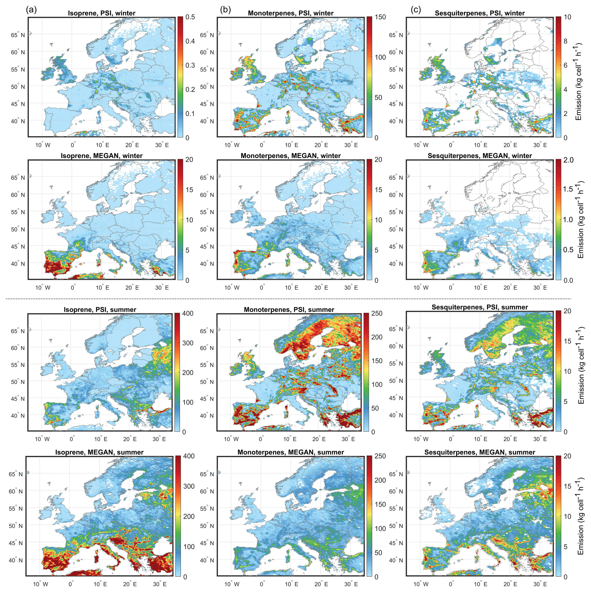
Figure 2Average hourly emissions of isoprene (a), monoterpenes (b), and sesquiterpenes (c) estimated by the PSI model and MEGAN2.1. The upper and lower panels represent winter and summer cases, respectively.
The diurnal variations in the isoprene and monoterpene emissions showed a peak around noon for both models (Fig. 3). In winter, the highest isoprene emissions occurred in central Europe (CE) for the PSI model, while this was in southern Europe (SE) for MEGAN (Fig. 3a). The main reason is PSI isoprene mainly came from Norway spruce in CE instead of deciduous trees in the south during wintertime. Comparison of the monoterpene emissions (Fig. 3b) with temperature and photosynthetically active radiation (PAR) (Fig. 3c) indicates that monoterpene emissions by the PSI model are mostly temperature-dependent while the influence of light is stronger for the MEGAN MT emissions. For instance, the highest PSI MT emissions in summer occurred at the same time of the highest temperature (13:00–14:00 UTC), while the occurrence of the highest MEGAN MT is close to the PAR peak (10:00–12:00 UTC). MEGAN showed steeper changes () due to a larger slope coefficient β value used in the exponential temperature response function, as well as potentially higher fraction of light-dependent MT emissions. Especially for monoterpenes in southern Europe (SE) in summer, the highest increase and decrease rates reached 43.8 % (at 05:00 UTC) and −57.1 % (at 18:00 UTC), respectively, while in the PSI model the hourly changes varied between 18.6 % (at 09:00 UTC) and −15.6 % (at 19:00 UTC).
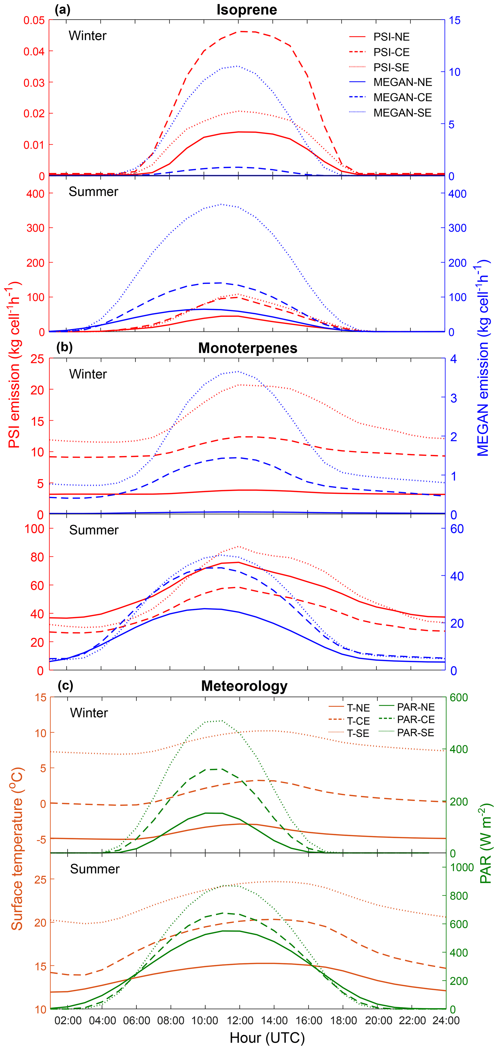
Figure 3Diurnal variations of average grid-scale isoprene (a), monoterpene emissions (b) in the model domain estimated by the PSI model (y axis left) and MEGAN2.1 (y axis right), and meteorological conditions (c). NE represents northern Europe, CE central Europe, and SE southern Europe.
BVOC measurements are rare and the concentrations are associated with very high spatial gradients (especially vertical) due to high reactivity and local mixing processes that are unlikely to be captured by the model in the respective grid cell. Nevertheless, with these caveats in mind, we compared a few measurements available for isoprene with our model results to get an idea about the range of differences. Compared to monoterpenes, there were more isoprene measurements at various European sites in 2011 (see Fig. 4). Clearly, the MEGAN isoprene data are much higher than measurements at all 12 sites while the PSI isoprene results are closer to the measurements.
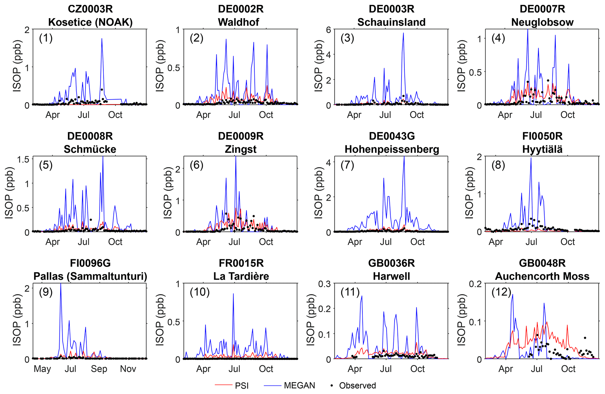
Figure 4Comparison between modelled and measured isoprene concentrations in 2011. The measurement data were obtained from the EBAS database (http://ebas.nilu.no/, last access: 12 March 2019) operated by Norwegian Institute for Air Research (NILU). The time resolution of measurements varies with sites: at station 9 FI0096G every 72 h, at stations 1–6 and 10 every 96 h, and at stations 7, 8, 11, and 12 every 3–12 h but averaged to 96 h for better visualisation.
Unlike the single compound of isoprene, monoterpenes consist of several species and therefore it is even more difficult to perform comparisons with these measurements, which are rare and have large uncertainties. Only a limited number of MT measurements were reported in Europe (only in Finland) during our simulation period (Hakola et al., 2012 Hellen et al., 2012). Hakola et al. (2012) reported average MT concentrations of about 508 ppt (with a range between about 150 and 800 ppt) in August 2011 at SMEAR II station at Hyytiälä. MEGAN MT for the same period was 117 ppt while PSI MT was around 2 ppb (for the same site Rinne et al. (2005) reported MT concentrations of between 200 and 500 ppt during daytime and more than 1 ppb at night-time in summer 2004). On the other hand, the measured MT concentrations at a nearby urban background station SMEAR III in Helsinki were lower, with around 117 ppt in summer (Hellen et al., 2012). Both models predicted higher concentrations for that site (MEGAN MT 303 ppt; PSI MT 1 ppb). In order to get an idea about the model performance in other regions, we also compared our results with MT concentrations measured at Hohenpeissenberg (southern Germany) in June 2006 (Oderbolz et al., 2013). Both model results (PSI MT: 75 ppt; MEGAN MT: 130 ppt) in that region were similar to measurements (∼100 ppt). Although this comparison of measurements and model results for different years under different meteorological conditions has a very high uncertainty, it might help to understand the range of differences between the model results and the measurements. In general, all these comparisons suggest that MT concentrations might be underestimated using MEGAN emissions over Scandinavia while PSI emissions might be too high. On the other hand, both models seem to predict MT emissions relatively well in central Europe.
These results generally agree with previous inter-comparison studies. Studies comparing different models with each other, as well as with measurements, suggest that MEGAN tends to overestimate isoprene emissions especially in Scandinavian countries and southwest Europe and to underestimate monoterpene emissions by more than a factor of 2 (Bash et al., 2016; Carlton and Baker, 2011; Emmerson et al., 2016; Poupkou et al., 2010; Silibello et al., 2017). However, due to limited measurement data and large uncertainties, and especially due to representativeness of measurement and modelled locations, it is not possible to conclude which model predicts more reliable BVOC emissions.
3.2 Influence of different BVOC emissions on the modelling of ozone and aerosols
3.2.1 Ozone
The modelled ozone mixing ratios from two simulations using the biogenic emissions calculated by the PSI model and MEGAN were evaluated by the measurements from the European air quality database (AirBase; Mol and Leeuw, 2005). Table 2 shows the statistical metrics of modelled average mixing ratios of afternoon (12:00–18:00 UTC) surface ozone at 537 rural background stations. The model performance in summer was generally better than in winter for all regions, but the difference between the PSI model and MEGAN was small. In winter, the two models showed similar mean bias (∼3 ppb) and RMSE (∼9.2 ppb) between modelled and measured concentrations. In summer, the PSI model showed lower (34.0 %) mean bias but slightly higher (1.3 %) RMSE than MEGAN. To investigate the difference in more detail, we compared the bias between modelled and observed O3 in different mixing ratio bins for different regions in summer (Fig. 5). In general, ozone modelled using the BVOC emission input from both models was overestimated at low mixing ratios and underestimated at high mixing ratios. A similar pattern was found in previous O3 modelling studies in Europe (Im et al., 2015; Oikonomakis et al., 2018; Solazzo et al., 2017). CAMx performed better with MEGAN emissions at most stations at the high ozone bins. Although the PSI model led to lower overall MB (Table 2), it was mostly due to compensation at the low- and high-O3 level bins.
Table 2Comparison between modelled and measured mean afternoon (12:00–18:00 UTC) mixing ratios of surface ozone at 537 rural AirBase stations. NE represents northern Europe, CE central Europe, and SE southern Europe. MB: mean bias; ME: mean error; RMSE: root-mean-square error; MFB: mean fractional bias; MFE: mean fractional error.

To further explore the reasons for the different model performance in the ozone simulations, we present the spatial distributions of modelled ozone in summer calculated using BVOC emissions from the PSI model and MEGAN in Fig. 6. PSI O3 was generally lower than MEGAN O3 across all of Europe. In summer, the largest effect of using different BVOC emissions on ozone was mostly in southern Europe, especially in the Mediterranean region, with the highest relative difference between PSI O3 and MEGAN O3 reaching −14 % (7.5 ppb, in Italy). On the other hand, in the UK and Ireland, where isoprene emissions by the PSI model were higher than MEGAN (Fig. S2), a positive difference up to 3.9 ppb was found. The spatial distribution of the ozone difference, i.e. (PSI O3)–(MEGAN O3) (Fig. 6c), is very similar to that of the difference in the isoprene emissions (Fig. S2a). As an important ozone precursor, isoprene reacts with hydroxyl radicals (OH) to form peroxyl radicals (RO2, HO2), which further react with NO to generate NO2 and finally ozone (Wennberg et al., 2018). This process can be significantly affected by the availability of isoprene and NOx in the atmosphere as well as temperature (Calfapietra et al., 2013), leading to high uncertainties in the net influence of BVOC emissions. Li et al. (2007) found that increasing the isoprene emissions by 50 % resulted in an increase in the O3 mixing ratios by 5–25 ppb in urban Houston in the United States, and Zare et al. (2012) suggested that the 21 % higher annual isoprene emissions by MEGAN than GEIA (Global Emissions Inventory Activity) led to up to 10 % higher O3 concentrations in the African savannah. However, the effect of the BVOC emissions on the ozone levels in Europe was much smaller in this study. The around 3 times higher isoprene emissions in MEGAN only led to up to ∼10 % (7 ppb) higher ozone mixing ratios in summer compared to the PSI model. Similarly, an earlier study by Aksoyoglu et al. (2012) using the PSI model for BVOC emissions suggested that increasing the isoprene emissions by a factor of 4 in Europe led to an increase of less than 10 % in the afternoon ozone mixing ratios. The main reason for the weak effect of the isoprene emissions on ozone is the stronger sensitivity of ozone formation in general to NOx emissions rather than VOC emissions in Europe. An additional reason might be the rather low ozone production compared to the background ozone, where the latter is not affected by local European emissions (Oikonomakis et al., 2018; Sartelet et al., 2012). Several European studies reported that ozone formation in most regions is NOx-sensitive, except around the English Channel, Benelux, and Po Valley regions, where NOx emissions are high (due to intensive anthropogenic NOx emissions from both land and shipping or geographical characteristics leading to high accumulation of pollutants) and the response to a change in the VOC emissions is relatively strong (Aksoyoglu et al., 2012; Beekmann and Vautard, 2010; Oikonomakis et al., 2018). However, the sensitivity of ozone formation to its precursor emissions might be changing as a result of large NOx emission reductions in Europe since 1990 according to the Gothenburg Protocol. On the other hand, emissions from shipping activities are not regulated as strictly as land emissions and have been increasing continuously, especially in the Mediterranean, affecting both ozone and particulate matter concentrations (Aksoyoglu et al., 2016; Viana et al., 2014).
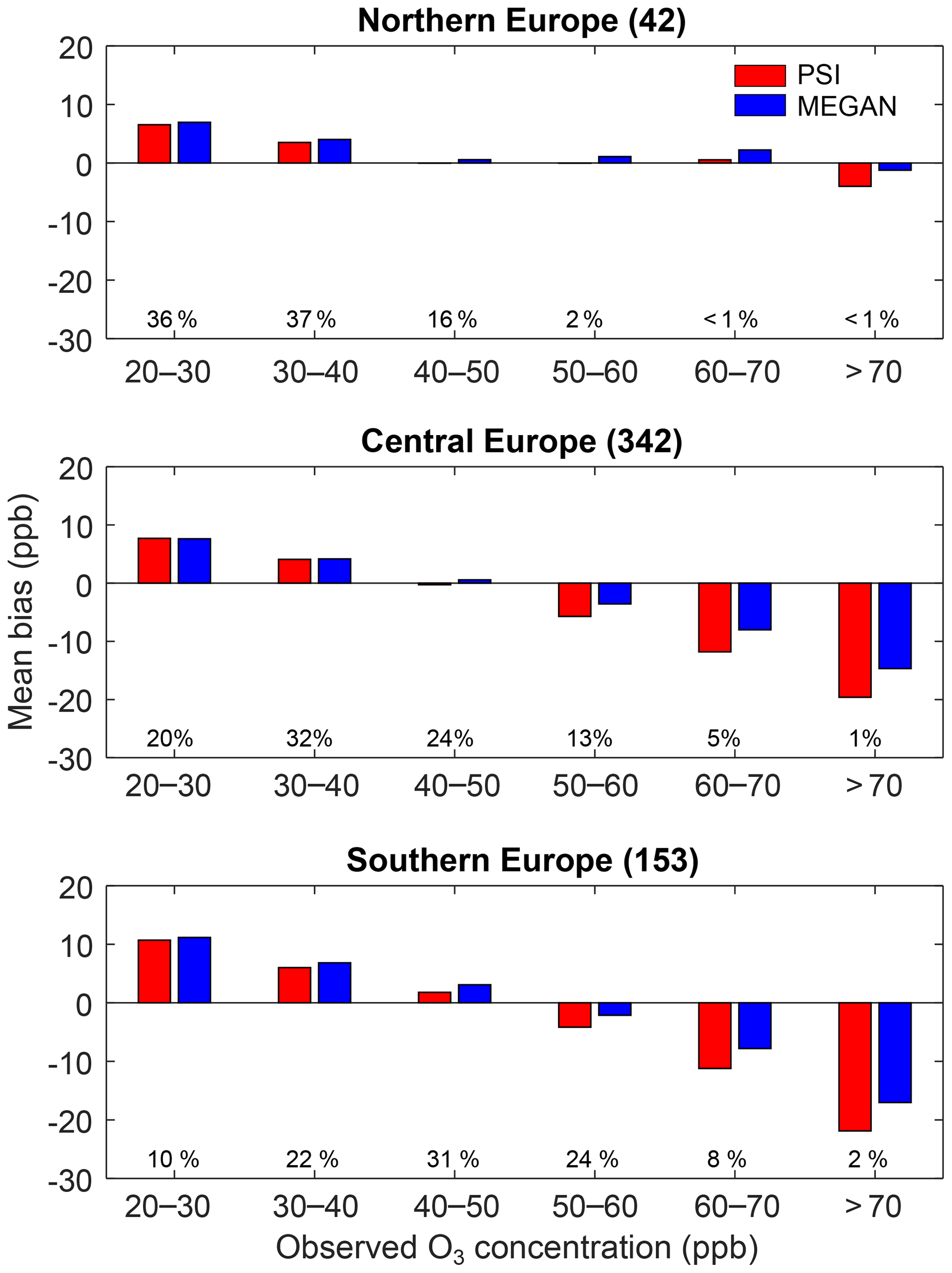
Figure 5Mean bias of surface O3 mixing ratios in the afternoon (12:00–18:00 UTC) for each bin of observed hourly average ozone in July 2011. The number of stations available for each region is reported in parentheses at the top of each panel. Percentage values below the bars show the relative fraction of data in each bin.
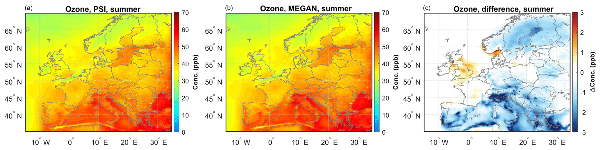
Figure 6Modelled afternoon (12:00–18:00 UTC) mixing ratios of surface ozone in summer using PSI emissions (PSI O3, a), MEGAN emissions (MEGAN O3, b), and the difference between PSI O3 and MEGAN O3 (c).
3.2.2 Organic aerosols
The effects of different BVOC emissions on organic aerosols were investigated by comparing modelled OA concentrations with measurements at nine ACSM/AMS stations. Although the OA concentrations were generally under-predicted in both cases, the model performance for OA was better with the PSI biogenic emissions (Fig. 7). About 67 % of the modelled OA concentrations were below the 1:2 line in the case of MEGAN (Fig. 7b). The mean bias between observed and modelled OA concentrations with the PSI BVOC emissions was lower than the bias obtained with MEGAN emissions (3.9 % in Paris and 83.4 % in Mace Head; see Table 3). The better model performance when using the PSI emissions was more obvious at rural or remote stations where biogenic sources play a major role in OA formation. The mean bias of OA by the PSI model was 21 % to 83 % lower than MEGAN at rural or remote stations (Finokalia, San Pietro Capofiume, Montsec, SMEAR II, and Mace Head), while the range was 4 %–12 % for Paris, Bologna, and Marseille (see Table 3). The situation of Zurich was different with an MB reduction of 67 % by the PSI model compared with MEGAN as an urban station, mostly because the station is an urban background site that is strongly affected by biogenic emissions (Daellenbach et al., 2017).
Table 3Statistical analysis of aerosols for different ACSM/AMS stations. MB: mean bias; ME: mean error; RMSE: root-mean-square error; MFB: mean fractional bias; MFE: mean fractional error.
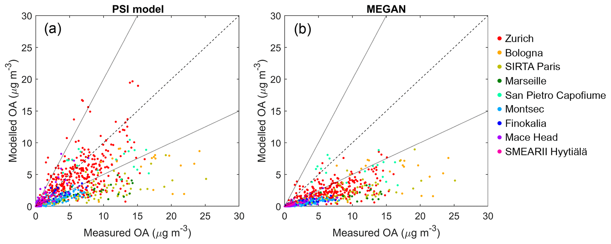
Figure 7Modelled versus measured daily OA concentrations using BVOC emissions calculated by the PSI model (PSI OA) (a) and MEGAN (MEGAN OA) (b) at nine ACSM/AMS stations. The dashed line represents the 1:1 line and dotted lines represent the 2:1 and 1:2 lines.
We further evaluated the model performance of the temporal variation at Zurich and Mace Head as examples of urban background and rural stations, respectively (Fig. 8, top row), because these two datasets covered almost the whole year. In spite of some underestimation, the temporal variation was well captured. At Zurich, the difference between the two cases (PSI OA and MEGAN OA) was small in February and March and they were both lower than the measurements, possibly due to underestimation of biomass burning OA (Fountoukis et al., 2014). The largest difference occurred in autumn when PSI OA reproduced the measurements quite well, while MEGAN OA showed a large underestimation. This is consistent with source apportionment studies performed for Zurich (Canonaco et al., 2013; Daellenbach et al., 2017) which reported that the contribution of biogenic sources to OA was minor in the period of January to March but significant (>50 %) in summer and autumn.
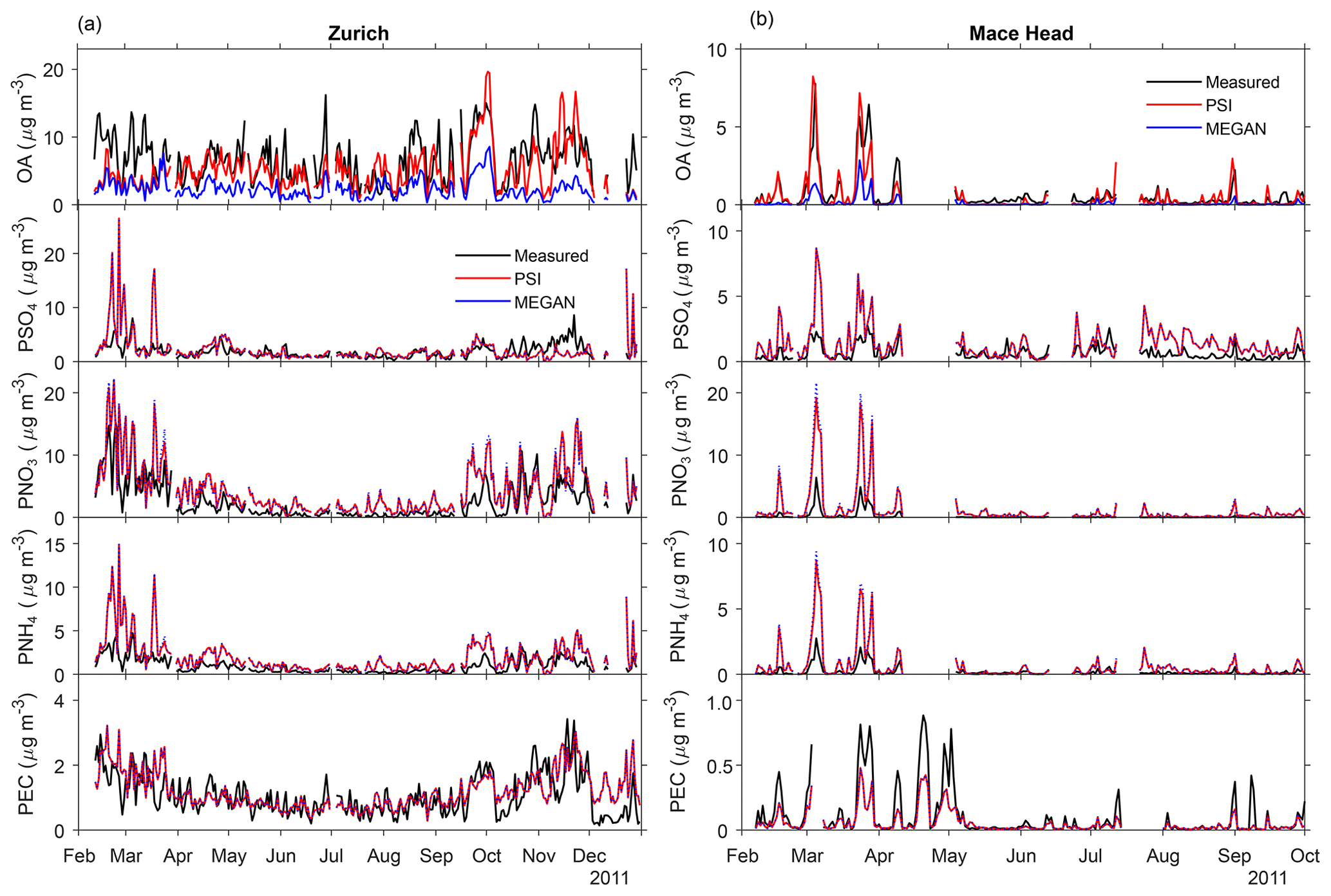
Figure 8Temporal variation in the modelled (with both PSI and MEGAN emissions) and measured concentrations of organic and inorganic aerosols at Zurich (a) and Mace Head (b) in 2011.
The situation was quite different for Mace Head. Located on the west coast of Ireland and 90 km away from the closest city Galway (Schmale et al., 2017), Mace Head is a remote station with low influence from anthropogenic activity (O'Dowd et al., 2014). The simulation with the PSI biogenic emission model could reproduce all the measured peaks quite well, while the simulation using the MEGAN emissions failed to capture their magnitude. To investigate the cause of the high OA concentrations during certain periods, 72 h back-trajectory analyses ending at Mace Head on 26 March (as an example for a high-OA day) and on 4 August (as an example for a low-OA day) were conducted by NOAA's HYSPLIT atmospheric transport and dispersion modelling system (Stein et al., 2015). According to the HYSPLIT results (Fig. S4), the air masses were transported from Ireland and Scotland during the high-OA period (Fig. S4a), while during the low-OA period the air masses came from the North Atlantic Ocean (Fig. S4b), suggesting that the OA peaks originated from anthropogenic or biogenic sources on land. The influence of wind direction was further studied by comparing modelled and measured OA during the two periods featured land-based wind (24–26 March) and marine-based wind (2–4 August) in Fig. S5. Measured OA in periods with dominant wind direction from land was higher than during the marine-based wind-dominant periods by a factor of ∼10. Modelled PSI OA was very close to measurements while MEGAN OA was underestimated in both periods. However, it is not possible to conclude that the good model performance for OA with PSI emissions is due to the fact that its high MT emissions are more accurate. It could also be due to the overestimated MT emissions compensating for other missing continental sources of OA, e.g. biomass burning.
The spatial distribution of the SOA difference showed a similar pattern as its main precursor, monoterpenes (Fig. 9). The PSI emissions lead to significantly higher SOA production than MEGAN (by 113 % and 109 % in winter and summer, respectively). The grid-scale difference reached up to a factor of 35 and 17 for winter and summer SOA, respectively. The largest differences occurred in central Europe, the Iberian Peninsula, and Turkey in winter, and especially in Scandinavia in summer.

Figure 9Modelled SOA concentrations using PSI emissions (PSI SOA) (a, b), MEGAN emissions (MEGAN SOA) (c, d), and the difference between PSI SOA and MEGAN SOA (e, f).
The modelled primary organic aerosol (POA) was also slightly higher (6.5 % in winter and 7.8 % in summer on average) in PSI emissions compared to the case with MEGAN (Fig. S6). Unlike in the traditional CTMs, where POA is treated as inert, the VBS scheme of CAMx allows POA to evaporate and react with oxidants. According to the partitioning theory (Donahue et al., 2006; Odum et al., 1996), higher total OA concentrations led to higher partitioning to the particle phase for all compounds that are soluble in the aerosol matrix. Therefore, in our case, the high PSI OA shifted the particle–gas equilibrium of primary condensable gases towards the particle phase, resulting in higher POA.
3.2.3 Inorganic aerosols
The influence of BVOC emissions on SIA was much smaller than on SOA according to the comparison of model results with measurements (Table 3). At the nine ACSM/AMS stations, using the PSI emissions generally reduced the RMSE between modelled and measured particulate nitrate (PNO3), sulfate (PSO4), and ammonium (PNH4) by up to 15.0 %, 1.7 %, and 7.7 %, respectively, compared to CAMx simulations with the MEGAN emissions. Only Finokalia (Greece, rural) and San Pietro Capofiume (Italy, rural) had lower RMSE in the MEGAN emissions. Unlike the obvious difference in OA, the difference between the modelled temporal variations of the inorganic aerosol was negligible with the two emission estimates (Fig. 8). MEGAN PNO3 was slightly higher than PSI because lower MT emission by MEGAN led to a lower MT–NO3 reaction and therefore more NOx was available to be oxidised to PNO3 (Fig. S7).
The modelled and measured daily average concentrations match well, except for February and March at Zurich, when temperature was significantly underestimated and resulted in higher condensation (Fig. S8a). A similar effect on temperature was not observed in OA during the same period, possibly due to compensation of underestimated winter OA as a consequence of lacking sources in the model, especially biomass burning (Ciarelli et al., 2017). On the other hand, the modelled primary elemental carbon (PEC) matched the measurements at Zurich very well.
Similar to the situation of OA, the measured SIA (PSO4, PNO3, and PNH4) at Mace Head peaked during the periods with wind from land. Both biogenic models captured the peaks well but overestimated the SIA during the peak periods. The modelled elemental carbon concentrations (PEC, in Fig. 8), on the other hand, were lower than the measured equivalent black carbon (EBC) in general but followed the temporal variation very well. In a study about the aerosols at Mace Head, O'Dowd et al. (2014) reported that EBC measurements can significantly overestimate black carbon concentration by up to 50 % or more. Overestimation of SIA could result from either precursor emissions that are too high or from too much particle formation in the aqueous phase. The precursor gases SO2 and NOx from anthropogenic sources (continental, shipping) (Fig. S7) might be accumulated too highly in the surface layer since all emissions were injected into the first layer, leading to SIA formation that is too high.
The differences in the spatial distributions of PSO4, PNO3, and PNH4 between the two simulations with PSI and MEGAN emissions are shown in Fig. 10. The inorganic aerosol concentrations varied by less than 15 % on the grid scale for the different BVOC emissions. The highest PSO4 levels were predicted in central and eastern Europe in winter, where SO2 emissions are higher, while in summer the elevated sulfate concentrations were mostly along the shipping routes (Fig. 10). The PSI BVOC emissions lead to higher PSO4 than MEGAN, especially over the area from southern Poland to Turkey through the Balkan Peninsula in summer. These regions have the highest SO2 emissions in the model domain due to large combustion-based power plants and coal burning. In summer, the main pathway for sulfate formation in southern Europe is the gas-phase oxidation of SO2 with OH radical (Chrit et al., 2018; Megaritis et al., 2013). The higher sulfate concentrations predicted by CAMx with PSI BVOC emissions are consistent with the spatial pattern of the differences between PSI and MEGAN simulations for SO2 concentrations and OH radicals (Fig. S9) due to the following reason: as reaction with OH radical is the largest loss pathway for isoprene in the atmosphere (Wennberg et al., 2018), higher isoprene emissions in MEGAN consume more OH radical. As a consequence, less SO2 is oxidised to form PSO4 when MEGAN emissions are used (Fig. S9), leading to lower PSO4 formation.
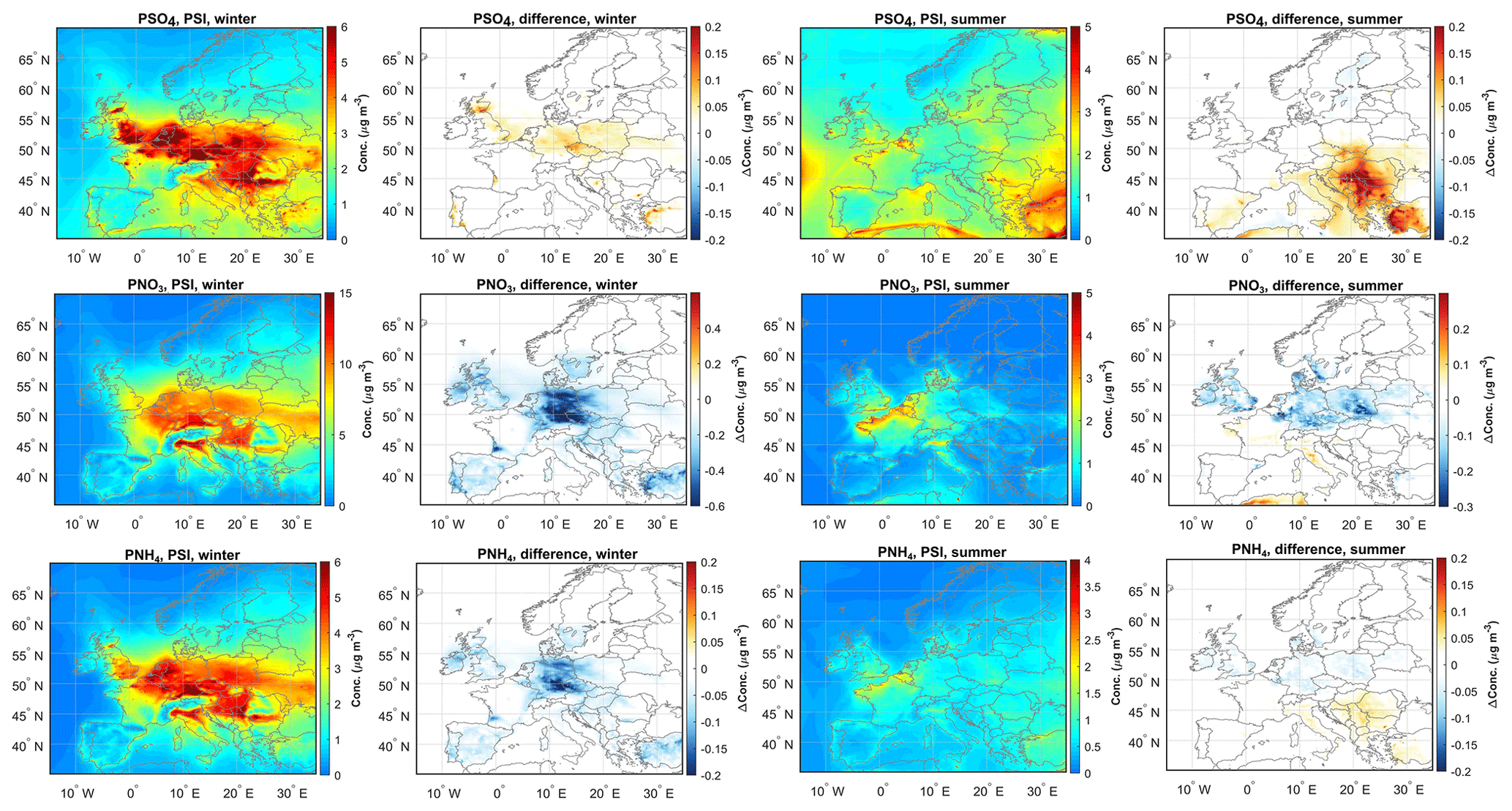
Figure 10Modelled secondary inorganic aerosol (SIA) concentrations using PSI emissions and the difference between PSI and MEGAN.
Formation of PNO3 depends on the availability of NOx and NH3 emissions (Aksoyoglu et al., 2011; Wen et al., 2015). In contrast to PSO4, PNO3, and PNH4 concentrations modelled using the PSI biogenic emissions were generally lower than those using MEGAN emissions, especially in regions where the PSI model has more MT emissions (Fig. S2b). Nitrate radicals are recognised as a significant sink for BVOCs, especially monoterpenes at night (while OH oxidation is more relevant for isoprene during daytime) (Kiendler-Scharr et al., 2016; Ng et al., 2017). Higher monoterpene emissions produced by the PSI model lead to larger consumption of nitrate radicals affecting PNO3 formation from HNO3 and NH3. These results are consistent with a recent study showing the significant effect of BVOCs on ammonium nitrate (Aksoyoglu et al., 2017).
In this study, European air quality in the year 2011 was simulated by the regional air quality model CAMx using two biogenic volatile organic compound (BVOC) emission models: MEGAN and PSI model. The model results were evaluated by O3 measurements from the European air quality database (AirBase v7), as well as the aerosol measurements at nine ACSM/AMS stations. The results indicate that MEGAN generates more isoprene (by a factor of about 3) but less (∼36 %) monoterpene emissions than the PSI model in Europe in summer, mainly due to their different vegetation classification and reference emission rates. In spite of much higher isoprene emissions, simulations with MEGAN only led to slightly higher (7 ppb, <10 %) ozone concentrations in summer compared to PSI emissions, especially in southern Europe. The evaluation of model results showed that PSI emissions improve the model performance for low ozone mixing ratios, but they worsen it at mixing ratios above 60 ppb.
The largest effect of using different BVOC emissions was predicted to be on SOA. PSI emissions led to higher SOA concentrations by about 110 % compared to MEGAN due to higher monoterpene emissions and therefore show a better model performance for OA at all nine measurement sites. A more detailed evaluation of modelled organic and inorganic aerosols was performed at Zurich and Mace Head, where aerosol measurements were available for relatively long periods. Comparison of modelled and measured OA at Zurich suggested that OA concentrations could be captured very well with PSI BVOC emissions most of the time except in winter when modelled OA was underestimated by both PSI and MEGAN emissions. These results pointed out the missing winter sources, such as biomass burning. On the other hand, at the remote site Mace Head, aerosol concentrations were affected by the prevailing air masses. Using PSI biogenic emissions, we could reproduce the OA peaks almost perfectly while OA concentrations were significantly underestimated when MEGAN biogenic emissions were used. One should, however, keep in mind that good model performance could also be due to the compensation for other factors.
Effects of using different BVOC emission models on secondary inorganic aerosols (particulate nitrate, sulfate, ammonium) were relatively small (<15 %). The mean bias between modelled and measured values was lower when the PSI model was used. The results of this study emphasise the importance of BVOC emissions in ozone and organic aerosol simulations and model inter-comparison studies. In future studies, emission factors should be improved in BVOC models to include more regional-specific vegetation types to reduce the uncertainties in BVOC emission estimates and to improve air quality modelling results.
Data related to this article are available online at https://doi.org/10.5281/zenodo.2598386 (Jiang and Aksoyoglu, 2019).
The supplement related to this article is available online at: https://doi.org/10.5194/acp-19-3747-2019-supplement.
JJ and SA initiated the study. JJ carried out the model simulation and data analysis. GC and EO contributed to model set-up. IEH, FC, COD, JO, and MCM provided the measurement data and contributed to data interpretation. SA, ASHP, and UB supervised the entire work development. The paper was prepared by JJ. All authors discussed and contributed to the final paper.
The authors declare that they have no conflict of interest.
We would like to thank the TNO for providing anthropogenic emissions, the
European Centre for Medium-Range Weather Forecasts (ECMWF) for the access to
the meteorological data, the European Environmental Agency (EEA) for the air
quality data, and the National Aeronautics and Space Administration (NASA) and
its data-contributing agencies (NCAR, UCAR) for the TOMS and MODIS data, the
global air quality model data, and the TUV model. Simulations of WRF and CAMx
models were performed at the Swiss National Supercomputing Centre (CSCS). We
thank the EBAS database of the Norwegian Institute for Air Research (NILU) for
the measurement data of isoprene concentration. We are grateful to RAMBOLL
for the valuable support for CAMx. We thank the ACSM/AMS data providers,
namely Stefania Gilardoni for the Bologna and San Pietro Capofiume stations,
Nicolas Marchand and the MASSALYA instrumental platform
(https://lce.univ-amu.fr/en/massalya, last access: 12 March 2019 for Marseille, Olivier Favez (INERIS) and the
whole SIRTA team for measurements conducted in the Paris area in the frame of
the EU FP7 ACTRIS programme under the grant agreement no. 262254, Kalliopi
Florou for Finokalia, and Liqing Hao and Annele Virtanen for SMEAR II
Hyytiälä. EPA-Ireland (AEROSOURCE, 2016-CCRP-MS-31) is acknowledged,
as well as EGAR group from IDAEA-CSIC (special mention to Anna Ripoll and
Andrés Alastuey) and Generalitat de Catalunya (AGAUR 2017 SGR41). María Cruz Minguillón acknowledges the Ramón y Cajal fellowship awarded by the
Spanish Ministry of Economy, Industry and Competitiveness.
Edited by: Ilona Riipinen
Reviewed by: three
anonymous referees
Aksoyoglu, S., Keller, J., Barmpadimos, I., Oderbolz, D., Lanz, V. A., Prévôt, A. S. H., and Baltensperger, U.: Aerosol modelling in Europe with a focus on Switzerland during summer and winter episodes, Atmos. Chem. Phys., 11, 7355–7373, https://doi.org/10.5194/acp-11-7355-2011, 2011.
Aksoyoglu, S., Keller, J., Oderbolz, D. C., Barmpadimos, I., Prévôt, A. S. H., and Baltensperger, U.: Sensitivity of ozone and aerosols to precursor emissions in Europe, Int. J. Environ. Pollut., 50, 451–459, https://doi.org/10.1504/ijep.2012.051215, 2012.
Aksoyoglu, S., Baltensperger, U., and Prévôt, A. S. H.: Contribution of ship emissions to the concentration and deposition of air pollutants in Europe, Atmos. Chem. Phys., 16, 1895–1906, https://doi.org/10.5194/acp-16-1895-2016, 2016.
Aksoyoglu, S., Ciarelli, G., El-Haddad, I., Baltensperger, U., and Prévôt, A. S. H.: Secondary inorganic aerosols in Europe: sources and the significant influence of biogenic VOC emissions, especially on ammonium nitrate, Atmos. Chem. Phys., 17, 7757–7773, https://doi.org/10.5194/acp-17-7757-2017, 2017.
Andreani-Aksoyoglu, S. and Keller, J.: Estimates of monoterpene and isoprene emissions from the forests in Switzerland, J. Atmos. Chem, 20, 71–87, https://doi.org/10.1007/bf01099919, 1995.
Ayres, B. R., Allen, H. M., Draper, D. C., Brown, S. S., Wild, R. J., Jimenez, J. L., Day, D. A., Campuzano-Jost, P., Hu, W., de Gouw, J., Koss, A., Cohen, R. C., Duffey, K. C., Romer, P., Baumann, K., Edgerton, E., Takahama, S., Thornton, J. A., Lee, B. H., Lopez-Hilfiker, F. D., Mohr, C., Wennberg, P. O., Nguyen, T. B., Teng, A., Goldstein, A. H., Olson, K., and Fry, J. L.: Organic nitrate aerosol formation via NO3 + biogenic volatile organic compounds in the southeastern United States, Atmos. Chem. Phys., 15, 13377–13392, https://doi.org/10.5194/acp-15-13377-2015, 2015.
Baldocchi, D. D., Hutchison, B. A., Matt, D. R., and McMillen, R. T.: Canopy radiative-transfer models for spherical and known leaf inclination angle distributions – a test in an oak hickory forest, J. Appl. Ecol., 22, 539–555, https://doi.org/10.2307/2403184, 1985.
Bash, J. O., Baker, K. R., and Beaver, M. R.: Evaluation of improved land use and canopy representation in BEIS v3.61 with biogenic VOC measurements in California, Geosci. Model Dev., 9, 2191–2207, https://doi.org/10.5194/gmd-9-2191-2016, 2016.
Beekmann, M. and Vautard, R.: A modelling study of photochemical regimes over Europe: robustness and variability, Atmos. Chem. Phys., 10, 10067–10084, https://doi.org/10.5194/acp-10-10067-2010, 2010.
Bessagnet, B., Pirovano, G., Mircea, M., Cuvelier, C., Aulinger, A., Calori, G., Ciarelli, G., Manders, A., Stern, R., Tsyro, S., García Vivanco, M., Thunis, P., Pay, M.-T., Colette, A., Couvidat, F., Meleux, F., Rouïl, L., Ung, A., Aksoyoglu, S., Baldasano, J. M., Bieser, J., Briganti, G., Cappelletti, A., D'Isidoro, M., Finardi, S., Kranenburg, R., Silibello, C., Carnevale, C., Aas, W., Dupont, J.-C., Fagerli, H., Gonzalez, L., Menut, L., Prévôt, A. S. H., Roberts, P., and White, L.: Presentation of the EURODELTA III intercomparison exercise – evaluation of the chemistry transport models' performance on criteria pollutants and joint analysis with meteorology, Atmos. Chem. Phys., 16, 12667–12701, https://doi.org/10.5194/acp-16-12667-2016, 2016.
Bicheron, P., Defourny, P., Brockmann, C., Schouten, L., Vancutsem, C., Huc, M., Bontemps, S., Leroy, M., Achard, F., Herold, M., Ranera, F., and Arino, O.: GLOBCOVER: Products Description and Validation Report, Medias France, Toulouse Cedex, France, 2008.
Bonn, B., von Kuhlmann, R., and Lawrence, M. G.: High contribution of biogenic hydroperoxides to secondary organic aerosol formation, Geophys. Res. Lett., 31, L10108, https://doi.org/10.1029/2003gl019172, 2004.
Bozzetti, C., El Haddad, I., Salameh, D., Daellenbach, K. R., Fermo, P., Gonzalez, R., Minguillón, M. C., Iinuma, Y., Poulain, L., Elser, M., Müller, E., Slowik, J. G., Jaffrezo, J.-L., Baltensperger, U., Marchand, N., and Prévôt, A. S. H.: Organic aerosol source apportionment by offline-AMS over a full year in Marseille, Atmos. Chem. Phys., 17, 8247–8268, https://doi.org/10.5194/acp-17-8247-2017, 2017.
Calfapietra, C., Fares, S., Manes, F., Morani, A., Sgrigna, G., and Loreto, F.: Role of Biogenic Volatile Organic Compounds (BVOC) emitted by urban trees on ozone concentration in cities: A review, Environ. Pollut., 183, 71–80, https://doi.org/10.1016/j.envpol.2013.03.012, 2013.
Cannell, M. G. R.: World forest biomass and primary production data, Academic Press, London, 1982.
Canonaco, F., Crippa, M., Slowik, J. G., Baltensperger, U., and Prévôt, A. S. H.: SoFi, an IGOR-based interface for the efficient use of the generalized multilinear engine (ME-2) for the source apportionment: ME-2 application to aerosol mass spectrometer data, Atmos. Meas. Tech., 6, 3649–3661, https://doi.org/10.5194/amt-6-3649-2013, 2013.
Carlton, A. G. and Baker, K. R.: Photochemical Modeling of the Ozark Isoprene Volcano: MEGAN, BEIS, and Their Impacts on Air Quality Predictions, Environ. Sci. Technol., 45, 4438–4445, https://doi.org/10.1021/es200050x, 2011.
Carlton, A. G., Pinder, R. W., Bhave, P. V., and Pouliot, G. A.: To What Extent Can Biogenic SOA be Controlled?, Environ. Sci. Technol., 44, 3376–3380, https://doi.org/10.1021/es903506b, 2010.
Chang, J. S., Brost, R. A., Isaksen, I. S. A., Madronich, S., Middleton, P., Stockwell, W. R., and Walcek, C. J.: A 3-dimensional Eulerian acid deposition model – physical concepts and formulation, J. Geophys. Res.-Atmos., 92, 14681–14700, https://doi.org/10.1029/JD092iD12p14681, 1987.
Chrit, M., Sartelet, K., Sciare, J., Pey, J., Nicolas, J. B., Marchand, N., Freney, E., Sellegri, K., Beekmann, M., and Dulac, F.: Aerosol sources in the western Mediterranean during summertime: a model-based approach, Atmos. Chem. Phys., 18, 9631–9659, https://doi.org/10.5194/acp-18-9631-2018, 2018.
Ciarelli, G., Aksoyoglu, S., Crippa, M., Jimenez, J.-L., Nemitz, E., Sellegri, K., Äijälä, M., Carbone, S., Mohr, C., O'Dowd, C., Poulain, L., Baltensperger, U., and Prévôt, A. S. H.: Evaluation of European air quality modelled by CAMx including the volatility basis set scheme, Atmos. Chem. Phys., 16, 10313–10332, https://doi.org/10.5194/acp-16-10313-2016, 2016.
Ciarelli, G., Aksoyoglu, S., El Haddad, I., Bruns, E. A., Crippa, M., Poulain, L., Äijälä, M., Carbone, S., Freney, E., O'Dowd, C., Baltensperger, U., and Prévôt, A. S. H.: Modelling winter organic aerosol at the European scale with CAMx: evaluation and source apportionment with a VBS parameterization based on novel wood burning smog chamber experiments, Atmos. Chem. Phys., 17, 7653–7669, https://doi.org/10.5194/acp-17-7653-2017, 2017.
Colette, A., Andersson, C., Manders, A., Mar, K., Mircea, M., Pay, M.-T., Raffort, V., Tsyro, S., Cuvelier, C., Adani, M., Bessagnet, B., Bergström, R., Briganti, G., Butler, T., Cappelletti, A., Couvidat, F., D'Isidoro, M., Doumbia, T., Fagerli, H., Granier, C., Heyes, C., Klimont, Z., Ojha, N., Otero, N., Schaap, M., Sindelarova, K., Stegehuis, A. I., Roustan, Y., Vautard, R., van Meijgaard, E., Vivanco, M. G., and Wind, P.: EURODELTA-Trends, a multi-model experiment of air quality hindcast in Europe over 1990–2010, Geosci. Model Dev., 10, 3255–3276, https://doi.org/10.5194/gmd-10-3255-2017, 2017.
Curci, G., Beekmann, M., Vautard, R., Smiatek, G., Steinbrecher, R., Theloke, J., and Friedrich, R.: Modelling study of the impact of isoprene and terpene biogenic emissions on European ozone levels, Atmos. Environ., 43, 1444–1455, https://doi.org/10.1016/j.atmosenv.2008.02.070, 2009.
Daellenbach, K. R., Stefenelli, G., Bozzetti, C., Vlachou, A., Fermo, P., Gonzalez, R., Piazzalunga, A., Colombi, C., Canonaco, F., Hueglin, C., Kasper-Giebl, A., Jaffrezo, J.-L., Bianchi, F., Slowik, J. G., Baltensperger, U., El-Haddad, I., and Prévôt, A. S. H.: Long-term chemical analysis and organic aerosol source apportionment at nine sites in central Europe: source identification and uncertainty assessment, Atmos. Chem. Phys., 17, 13265–13282, https://doi.org/10.5194/acp-17-13265-2017, 2017.
Dee, D. P., Uppala, S. M., Simmons, A. J., Berrisford, P., Poli, P., Kobayashi, S., Andrae, U., Balmaseda, M. A., Balsamo, G., Bauer, P., Bechtold, P., Beljaars, A. C. M., van de Berg, L., Bidlot, J., Bormann, N., Delsol, C., Dragani, R., Fuentes, M., Geer, A. J., Haimberger, L., Healy, S. B., Hersbach, H., Holm, E. V., Isaksen, L., Kallberg, P., Kohler, M., Matricardi, M., McNally, A. P., Monge-Sanz, B. M., Morcrette, J. J., Park, B. K., Peubey, C., de Rosnay, P., Tavolato, C., Thepaut, J. N., and Vitart, F.: The ERA-Interim reanalysis: configuration and performance of the data assimilation system, Q. J. Roy. Meteor. Soc., 137, 553–597, https://doi.org/10.1002/qj.828, 2011.
Donahue, N. M., Robinson, A. L., Stanier, C. O., and Pandis, S. N.: Coupled Partitioning, Dilution, and Chemical Aging of Semivolatile Organics, Environ. Sci. Technol., 40, 2635–2643, https://doi.org/10.1021/es052297c, 2006.
Duhl, T. R., Helmig, D., and Guenther, A.: Sesquiterpene emissions from vegetation: a review, Biogeosciences, 5, 761–777, https://doi.org/10.5194/bg-5-761-2008, 2008.
Emmerson, K. M., Galbally, I. E., Guenther, A. B., Paton-Walsh, C., Guerette, E.-A., Cope, M. E., Keywood, M. D., Lawson, S. J., Molloy, S. B., Dunne, E., Thatcher, M., Karl, T., and Maleknia, S. D.: Current estimates of biogenic emissions from eucalypts uncertain for southeast Australia, Atmos. Chem. Phys., 16, 6997–7011, https://doi.org/10.5194/acp-16-6997-2016, 2016.
Fountoukis, C., Megaritis, A. G., Skyllakou, K., Charalampidis, P. E., Pilinis, C., Denier van der Gon, H. A. C., Crippa, M., Canonaco, F., Mohr, C., Prévôt, A. S. H., Allan, J. D., Poulain, L., Petäjä, T., Tiitta, P., Carbone, S., Kiendler-Scharr, A., Nemitz, E., O'Dowd, C., Swietlicki, E., and Pandis, S. N.: Organic aerosol concentration and composition over Europe: insights from comparison of regional model predictions with aerosol mass spectrometer factor analysis, Atmos. Chem. Phys., 14, 9061–9076, https://doi.org/10.5194/acp-14-9061-2014, 2014.
Fu, P. Q., Kawamura, K., Chen, J., and Miyazaki, Y.: Secondary Production of Organic Aerosols from Biogenic VOCs over Mt. Fuji, Japan, Environ. Sci. Technol., 48, 8491–8497, https://doi.org/10.1021/es500794d, 2014.
Gilardoni, S., Massoli, P., Giulianelli, L., Rinaldi, M., Paglione, M., Pollini, F., Lanconelli, C., Poluzzi, V., Carbone, S., Hillamo, R., Russell, L. M., Facchini, M. C., and Fuzzi, S.: Fog scavenging of organic and inorganic aerosol in the Po Valley, Atmos. Chem. Phys., 14, 6967–6981, https://doi.org/10.5194/acp-14-6967-2014, 2014.
Griffin, R. J., Cocker, D. R., Seinfeld, J. H., and Dabdub, D.: Estimate of global atmospheric organic aerosol from oxidation of biogenic hydrocarbons, Geophys. Res. Lett., 26, 2721–2724, https://doi.org/10.1029/1999gl900476, 1999.
Grote, R. and Niinemets, U.: Modeling volatile isoprenoid emissions – a story with split ends, Plant Biology, 10, 8–28, https://doi.org/10.1055/s-2007-964975, 2008.
Guenther, A., Hewitt, C. N., Erickson, D., Fall, R., Geron, C., Graedel, T., Harley, P., Klinger, L., Lerdau, M., McKay, W. A., Pierce, T., Scholes, B., Steinbrecher, R., Tallamraju, R., Taylor, J., and Zimmerman, P.: A global-model of natural volatile organic-compound emissions, J. Geophys. Res.-Atmos., 100, 8873–8892, https://doi.org/10.1029/94jd02950, 1995.
Guenther, A., Baugh, B., Brasseur, G., Greenberg, J., Harley, P., Klinger, L., Serca, D., and Vierling, L.: Isoprene emission estimates and uncertainties for the Central African EXPRESSO study domain, J. Geophys. Res.-Atmos., 104, 30625–30639, https://doi.org/10.1029/1999jd900391, 1999.
Guenther, A., Karl, T., Harley, P., Wiedinmyer, C., Palmer, P. I., and Geron, C.: Estimates of global terrestrial isoprene emissions using MEGAN (Model of Emissions of Gases and Aerosols from Nature), Atmos. Chem. Phys., 6, 3181–3210, https://doi.org/10.5194/acp-6-3181-2006, 2006.
Guenther, A. B., Zimmerman, P. R., Harley, P. C., Monson, R. K., and Fall, R.: Isoprene and monoterpene emission rate variability – model evaluations and sensitivity analyses, J. Geophys. Res.-Atmos., 98, 12609–12617, https://doi.org/10.1029/93jd00527, 1993.
Guenther, A. B., Jiang, X., Heald, C. L., Sakulyanontvittaya, T., Duhl, T., Emmons, L. K., and Wang, X.: The Model of Emissions of Gases and Aerosols from Nature version 2.1 (MEGAN2.1): an extended and updated framework for modeling biogenic emissions, Geosci. Model Dev., 5, 1471–1492, https://doi.org/10.5194/gmd-5-1471-2012, 2012.
Hakola, H., Hellén, H., Hemmilä, M., Rinne, J., and Kulmala, M.: In situ measurements of volatile organic compounds in a boreal forest, Atmos. Chem. Phys., 12, 11665–11678, https://doi.org/10.5194/acp-12-11665-2012, 2012.
Hallquist, M., Wenger, J. C., Baltensperger, U., Rudich, Y., Simpson, D., Claeys, M., Dommen, J., Donahue, N. M., George, C., Goldstein, A. H., Hamilton, J. F., Herrmann, H., Hoffmann, T., Iinuma, Y., Jang, M., Jenkin, M. E., Jimenez, J. L., Kiendler-Scharr, A., Maenhaut, W., McFiggans, G., Mentel, Th. F., Monod, A., Prévôt, A. S. H., Seinfeld, J. H., Surratt, J. D., Szmigielski, R., and Wildt, J.: The formation, properties and impact of secondary organic aerosol: current and emerging issues, Atmos. Chem. Phys., 9, 5155–5236, https://doi.org/10.5194/acp-9-5155-2009, 2009.
Hantson, S., Knorr, W., Schurgers, G., Pugh, T. A. M., and Arneth, A.: Global isoprene and monoterpene emissions under changing climate, vegetation, CO2 and land use, Atmos. Environ., 155, 35–45, https://doi.org/10.1016/j.atmosenv.2017.02.010, 2017.
Hellen, H., Tykka, T., and Hakola, H.: Importance of monoterpenes and isoprene in urban air in northern Europe, Atmos. Environ., 59, 59–66, https://doi.org/10.1016/j.atmosenv.2012.04.049, 2012.
Hildebrandt, L., Engelhart, G. J., Mohr, C., Kostenidou, E., Lanz, V. A., Bougiatioti, A., DeCarlo, P. F., Prevot, A. S. H., Baltensperger, U., Mihalopoulos, N., Donahue, N. M., and Pandis, S. N.: Aged organic aerosol in the Eastern Mediterranean: the Finokalia Aerosol Measurement Experiment – 2008, Atmos. Chem. Phys., 10, 4167–4186, https://doi.org/10.5194/acp-10-4167-2010, 2010.
Hildebrandt Ruiz, L. and Yarwood, G.: Interactions between organic aerosol and NOy: Influence on oxidant production, University of Texas at Austin, ENVIRON International Corporation, Novato, CA, available at: http://aqrp.ceer.utexas.edu/projectinfoFY12_13\%5C12-012\%5C12-012\%20Final\%20Report.pdf (last access: 12 March 2019), 2013.
Hodzic, A., Kasibhatla, P. S., Jo, D. S., Cappa, C. D., Jimenez, J. L., Madronich, S., and Park, R. J.: Rethinking the global secondary organic aerosol (SOA) budget: stronger production, faster removal, shorter lifetime, Atmos. Chem. Phys., 16, 7917–7941, https://doi.org/10.5194/acp-16-7917-2016, 2016.
Hoffmann, T., Odum, J. R., Bowman, F., Collins, D., Klockow, D., Flagan, R. C., and Seinfeld, J. H.: Formation of organic aerosols from the oxidation of biogenic hydrocarbons, J. Atmos. Chem, 26, 189–222, https://doi.org/10.1023/a:1005734301837, 1997.
Horowitz, L. W., Walters, S., Mauzerall, D. L., Emmons, L. K., Rasch, P. J., Granier, C., Tie, X. X., Lamarque, J. F., Schultz, M. G., Tyndall, G. S., Orlando, J. J., and Brasseur, G. P.: A global simulation of tropospheric ozone and related tracers: Description and evaluation of MOZART, version 2, J. Geophys. Res.-Atmos., 108, 4784, https://doi.org/10.1029/2002jd002853, 2003.
Hoyle, C. R., Boy, M., Donahue, N. M., Fry, J. L., Glasius, M., Guenther, A., Hallar, A. G., Huff Hartz, K., Petters, M. D., Petäjä, T., Rosenoern, T., and Sullivan, A. P.: A review of the anthropogenic influence on biogenic secondary organic aerosol, Atmos. Chem. Phys., 11, 321–343, https://doi.org/10.5194/acp-11-321-2011, 2011.
Im, U., Bianconi, R., Solazzo, E., Kioutsioukis, I., Badia, A., Balzarini, A., Baro, R., Bellasio, R., Brunner, D., Chemel, C., Curci, G., Flemming, J., Forkel, R., Giordano, L., Jimenez-Guerrero, P., Hirtl, M., Hodzic, A., Honzak, L., Jorba, O., Knote, C., Kuenen, J. J. P., Makar, P. A., Manders-Groot, A., Neal, L., Perez, J. L., Pirovano, G., Pouliot, G., San Jose, R., Savage, N., Schroder, W., Sokhi, R. S., Syrakov, D., Torian, A., Tuccella, P., Werhahn, J., Wolke, R., Yahya, K., Zabkar, R., Zhang, Y., Zhang, J., Hogrefe, C., and Galmarini, S.: Evaluation of operational on-line-coupled regional air quality models over Europe and North America in the context of AQMEII phase 2. Part I: Ozone, Atmos. Environ., 115, 404–420, https://doi.org/10.1016/j.atmosenv.2014.09.042, 2015.
Jiang, J. and Aksoyoglu, S.: Dataset for “Effects of two different biogenic emission models on modelled ozone and aerosol concentrations in Europe”, Data set, Zenodo, https://doi.org/10.5281/zenodo.2598386, 2019.
Joss, U.: Mikrometeorologie, Profile und Flüsse von CO2, H2O, NO2, O3 in zwei mitteleuropäischen Nadelwäldern, PhD Thesis, University of Basel, Basel, Switzerland, 1995.
Karambelas, A.: The interactions of biogenic and anthropogenic gaseous emissions with respect to aerosol formation in the united states, Master of Science, Department of Atmospheric and Oceanic Sciences, University of Wisconsin, Madison, 2013.
Karl, M., Guenther, A., Köble, R., Leip, A., and Seufert, G.: A new European plant-specific emission inventory of biogenic volatile organic compounds for use in atmospheric transport models, Biogeosciences, 6, 1059–1087, https://doi.org/10.5194/bg-6-1059-2009, 2009.
Keenan, T., Niinemets, Ü., Sabate, S., Gracia, C., and Peñuelas, J.: Process based inventory of isoprenoid emissions from European forests: model comparisons, current knowledge and uncertainties, Atmos. Chem. Phys., 9, 4053–4076, https://doi.org/10.5194/acp-9-4053-2009, 2009.
Keller, A., Andreani-aksoyoglu, S., and Joss, U.: Inventory of natural emissions in Switzerland, in: Air Pollution III, Volume 2, Air Pollution Engineering and Management, edited by: Power, H., Moussiopoulos, N., and Brebbia C. A., Computational Mechanics Publications, Southampton, UK, 339–346, 1995.
Kesselmeier, J. and Staudt, M.: Biogenic Volatile Organic Compounds (VOC): An Overview on Emission, Physiology and Ecology, J. Atmos. Chem, 33, 23–88, https://doi.org/10.1023/a:1006127516791, 1999.
Kiendler-Scharr, A., Mensah, A. A., Friese, E., Topping, D., Nemitz, E., Prévôt, A. S. H., Aijala, M., Allan, J., Canonaco, F., Canagaratna, M., Carbone, S., Crippa, M., Dall Osto, M., Day, D. A., De Carlo, P., Di Marco, C. F., Elbern, H., Eriksson, A., Freney, E., Hao, L., Herrmann, H., Hildebrandt, L., Hillamo, R., Jimenez, J. L., Laaksonen, A., McFiggans, G., Mohr, C., O'Dowd, C., Otjes, R., Ovadnevaite, J., Pandis, S. N., Poulain, L., Schlag, P., Sellegri, K., Swietlicki, E., Tiitta, P., Vermeulen, A., Wahner, A., Worsnop, D., and Wu, H. C.: Ubiquity of organic nitrates from nighttime chemistry in the European submicron aerosol, Geophys. Res. Lett., 43, 7735–7744, https://doi.org/10.1002/2016gl069239, 2016.
Kirkby, J., Duplissy, J., Sengupta, K., Frege, C., Gordon, H., Williamson, C., Heinritzi, M., Simon, M., Yan, C., Almeida, J., Trostl, J., Nieminen, T., Ortega, I. K., Wagner, R., Adamov, A., Amorim, A., Bernhammer, A. K., Bianchi, F., Breitenlechner, M., Brilke, S., Chen, X. M., Craven, J., Dias, A., Ehrhart, S., Flagan, R. C., Franchin, A., Fuchs, C., Guida, R., Hakala, J., Hoyle, C. R., Jokinen, T., Junninen, H., Kangasluoma, J., Kim, J., Krapf, M., Kurten, A., Laaksonen, A., Lehtipalo, K., Makhmutov, V., Mathot, S., Molteni, U., Onnela, A., Perakyla, O., Piel, F., Petaja, T., Praplan, A. P., Pringle, K., Rap, A., Richards, N. A. D., Riipinen, I., Rissanen, M. P., Rondo, L., Sarnela, N., Schobesberger, S., Scott, C. E., Seinfeld, J. H., Sipila, M., Steiner, G., Stozhkov, Y., Stratmann, F., Tome, A., Virtanen, A., Vogel, A. L., Wagner, A. C., Wagner, P. E., Weingartner, E., Wimmer, D., Winkler, P. M., Ye, P. L., Zhang, X., Hansel, A., Dommen, J., Donahue, N. M., Worsnop, D. R., Baltensperger, U., Kulmala, M., Carslaw, K. S., and Curtius, J.: Ion-induced nucleation of pure biogenic particles, Nature, 533, 521–526, https://doi.org/10.1038/nature17953, 2016.
Koo, B., Knipping, E., and Yarwood, G.: 1.5-Dimensional volatility basis set approach for modeling organic aerosol in CAMx and CMAQ, Atmos. Environ., 95, 158–164, https://doi.org/10.1016/j.atmosenv.2014.06.031, 2014.
Kortelainen, A., Hao, L. Q., Tiitta, P., Jaatinen, A., Miettinen, P., Kulmala, M., Smith, J. N., Laaksonen, A., Worsnop, D. R., and Virtanen, A.: Sources of particulate organic nitrates in the boreal forest in Finland, Boreal Environ. Res., 22, 13–26, 2017.
Kuenen, J. J. P., Visschedijk, A. J. H., Jozwicka, M., and Denier van der Gon, H. A. C.: TNO-MACC_II emission inventory; a multi-year (2003–2009) consistent high-resolution European emission inventory for air quality modelling, Atmos. Chem. Phys., 14, 10963–10976, https://doi.org/10.5194/acp-14-10963-2014, 2014.
Lamb, B., Gay, D., Westberg, H., and Pierce, T.: A biogenic hydrocarbon emission inventory for the U.S.A. using a simple forest canopy model, Atmos. Environ. A-Gen., 27, 1673–1690, https://doi.org/10.1016/0960-1686(93)90230-V, 1993.
Lamb, B., Pierce, T., Baldocchi, D., Allwine, E., Dilts, S., Westberg, H., Geron, C., Guenther, A., Klinger, L., Harley, P., and Zimmerman, P.: Evaluation of forest canopy models for estimating isoprene emissions, J. Geophys. Res.-Atmos., 101, 22787–22797, https://doi.org/10.1029/96jd00056, 1996.
Li, G. H., Zhang, R. Y., Fan, J. W., and Tie, X. X.: Impacts of biogenic emissions on photochemical ozone production in Houston, Texas, J. Geophys. Res.-Atmos., 112, D10309, https://doi.org/10.1029/2006jd007924, 2007.
Megaritis, A. G., Fountoukis, C., Charalampidis, P. E., Pilinis, C., and Pandis, S. N.: Response of fine particulate matter concentrations to changes of emissions and temperature in Europe, Atmos. Chem. Phys., 13, 3423–3443, https://doi.org/10.5194/acp-13-3423-2013, 2013.
Messina, P., Lathière, J., Sindelarova, K., Vuichard, N., Granier, C., Ghattas, J., Cozic, A., and Hauglustaine, D. A.: Global biogenic volatile organic compound emissions in the ORCHIDEE and MEGAN models and sensitivity to key parameters, Atmos. Chem. Phys., 16, 14169–14202, https://doi.org/10.5194/acp-16-14169-2016, 2016.
Mol, W. and Leeuw, F.: AirBase: a valuable tool in air quality assessments, Proceedings of the 5th International Conference on Urban Air Quality, Valencia, Spain, 2005.
NCAR: The Tropospheric Visible and Ultraviolet (TUV) Radiation Model web page, National Center for Atmospheric Research, Atmospheric Chemistry Division, Boulder, Colorado, 2011.
NCAR: Weather Research and Forecasting Model WRF-ARW Version 3 Modeling System User's Guide, National Center for Atmospheric Research, Boulder, Colorado, USA, 2016.
Nenes, A., Pandis, S. N., and Pilinis, C.: ISORROPIA: A new thermodynamic equilibrium model for multiphase multicomponent inorganic aerosols, Aquat. Geochem., 4, 123–152, https://doi.org/10.1023/a:1009604003981, 1998.
Ng, N. L., Brown, S. S., Archibald, A. T., Atlas, E., Cohen, R. C., Crowley, J. N., Day, D. A., Donahue, N. M., Fry, J. L., Fuchs, H., Griffin, R. J., Guzman, M. I., Herrmann, H., Hodzic, A., Iinuma, Y., Jimenez, J. L., Kiendler-Scharr, A., Lee, B. H., Luecken, D. J., Mao, J., McLaren, R., Mutzel, A., Osthoff, H. D., Ouyang, B., Picquet-Varrault, B., Platt, U., Pye, H. O. T., Rudich, Y., Schwantes, R. H., Shiraiwa, M., Stutz, J., Thornton, J. A., Tilgner, A., Williams, B. J., and Zaveri, R. A.: Nitrate radicals and biogenic volatile organic compounds: oxidation, mechanisms, and organic aerosol, Atmos. Chem. Phys., 17, 2103–2162, https://doi.org/10.5194/acp-17-2103-2017, 2017.
O'Dowd, C., Ceburnis, D., Ovadnevaite, J., Vaishya, A., Rinaldi, M., and Facchini, M. C.: Do anthropogenic, continental or coastal aerosol sources impact on a marine aerosol signature at Mace Head?, Atmos. Chem. Phys., 14, 10687–10704, https://doi.org/10.5194/acp-14-10687-2014, 2014.
Oderbolz, D. C., Aksoyoglu, S., Keller, J., Barmpadimos, I., Steinbrecher, R., Skjøth, C. A., Plaß-Dülmer, C., and Prévôt, A. S. H.: A comprehensive emission inventory of biogenic volatile organic compounds in Europe: improved seasonality and land-cover, Atmos. Chem. Phys., 13, 1689–1712, https://doi.org/10.5194/acp-13-1689-2013, 2013.
Odum, J. R., Hoffmann, T., Bowman, F., Collins, D., Flagan, R. C., and Seinfeld, J. H.: Gas/particle partitioning and secondary organic aerosol yields, Environ. Sci. Technol., 30, 2580–2585, https://doi.org/10.1021/es950943+, 1996.
Oikonomakis, E., Aksoyoglu, S., Ciarelli, G., Baltensperger, U., and Prévôt, A. S. H.: Low modeled ozone production suggests underestimation of precursor emissions (especially NOx) in Europe, Atmos. Chem. Phys., 18, 2175–2198, https://doi.org/10.5194/acp-18-2175-2018, 2018.
Ovadnevaite, J., Ceburnis, D., Leinert, S., Dall'Osto, M., Canagaratna, M., O'Doherty, S., Berresheim, H., and O'Dowd, C.: Submicron NE Atlantic marine aerosol chemical composition and abundance: Seasonal trends and air mass categorization, J. Geophys. Res.-Atmos., 119, 11850–11863, https://doi.org/10.1002/2013jd021330, 2014.
Passant, N. R.: Speciation of UK emissions of non-methane volatile organic compounds, AEA Technology, Culham, Abingdon, Oxon, UK, 2002.
Petit, J.-E., Favez, O., Sciare, J., Crenn, V., Sarda-Estéve, R., Bonnaire, N., Mocnik, G., Dupont, J.-C., Haeffelin, M., and Leoz-Garziandia, E.: Two years of near real-time chemical composition of submicron aerosols in the region of Paris using an Aerosol Chemical Speciation Monitor (ACSM) and a multi-wavelength Aethalometer, Atmos. Chem. Phys., 15, 2985–3005, https://doi.org/10.5194/acp-15-2985-2015, 2015.
Poupkou, A., Giannaros, T., Markakis, K., Kioutsioukis, I., Curci, G., Melas, D., and Zerefos, C.: A model for European Biogenic Volatile Organic Compound emissions: Software development and first validation, Environ. Modell. Softw., 25, 1845–1856, https://doi.org/10.1016/j.envsoft.2010.05.004, 2010.
Rinne, J., Ruuskanen, T. M., Reissell, A., Taipale, R., Hakola, H., and Kulmala, M.: On-line PTR-MS measurements of atmospheric concentrations of volatile organic compounds in a European boreal forest ecosystem, Boreal Environ. Res., 10, 425–436, 2005.
Ripoll, A., Minguillón, M. C., Pey, J., Jimenez, J. L., Day, D. A., Sosedova, Y., Canonaco, F., Prévôt, A. S. H., Querol, X., and Alastuey, A.: Long-term real-time chemical characterization of submicron aerosols at Montsec (southern Pyrenees, 1570 m a.s.l.), Atmos. Chem. Phys., 15, 2935–2951, https://doi.org/10.5194/acp-15-2935-2015, 2015.
Rosenkranz, M., Pugh, T. A. M., Schnitzler, J. P., and Arneth, A.: Effect of land-use change and management on biogenic volatile organic compound emissions – selecting climate-smart cultivars, Plant Cell Environ., 38, 1896–1912, https://doi.org/10.1111/pce.12453, 2015.
Sartelet, K. N., Couvidat, F., Seigneur, C., and Roustan, Y.: Impact of biogenic emissions on air quality over Europe and North America, Atmos. Environ., 53, 131–141, https://doi.org/10.1016/j.atmosenv.2011.10.046, 2012.
Satoo, T. and Madgwick, H. A.: Forest Biomass, Martinus Nijhoff/Dr W. Junk Publishers, The Hague, 1982.
Schmale, J., Henning, S., Henzing, B., Keskinen, H., Sellegri, K., Ovadnevaite, J., Bougiatioti, A., Kalivitis, N., Stavroulas, I., Jefferson, A., Park, M., Schlag, P., Kristensson, A., Iwamoto, Y., Pringle, K., Reddington, C., Aalto, P., Äijälä, M., Baltensperger, U., Bialek, J., Birmili, W., Bukowiecki, N., Ehn, M., Fjæraa, A. M., Fiebig, M., Frank, G., Fröhlich, R., Frumau, A., Furuya, M., Hammer, E., Heikkinen, L., Herrmann, E., Holzinger, R., Hyono, H., Kanakidou, M., Kiendler-Scharr, A., Kinouchi, K., Kos, G., Kulmala, M., Mihalopoulos, N., Motos, G., Nenes, A., O'Dowd, C., Paramonov, M., Petäjä, T., Picard, D., Poulain, L., Prévôt, A. S. H., Slowik, J., Sonntag, A., Swietlicki, E., Svenningsson, B., Tsurumaru, H., Wiedensohler, A., Wittbom, C., Ogren, J. A., Matsuki, A., Yum, S. S., Myhre, C. L., Carslaw, K., Stratmann, F., and Gysel, M.: Collocated observations of cloud condensation nuclei, particle size distributions, and chemical composition, Sci. Data, 4, 170003, https://doi.org/10.1038/sdata.2017.3, 2017.
Schürmann, W.: Emission von Monoterpenen aus Nadeln von Picea Abies (L.) Karst, sowie deren Verhalten in der Atmosphäre, PhD Thesis, Technische Universität München, München, 1993.
Silibello, C., Baraldi, R., Rapparini, F., Facini, O., Neri, L., Brilli, F., Fares, S., Finardi, S., Magliulo, E., Ciccioli, P., and Ciccioli, P.: Modelling of biogenic volatile organic compounds emissions over italy, 18th International Conference on Harmonisation within Atmospheric Dispersion Modelling for Regulatory Purposes (HARMO), Bologna, Italy, 2017.
Simpson, D., Winiwarter, W., Borjesson, G., Cinderby, S., Ferreiro, A., Guenther, A., Hewitt, C. N., Janson, R., Khalil, M. A. K., Owen, S., Pierce, T. E., Puxbaum, H., Shearer, M., Skiba, U., Steinbrecher, R., Tarrason, L., and Oquist, M. G.: Inventorying emissions from nature in Europe, J. Geophys. Res.-Atmos., 104, 8113–8152, https://doi.org/10.1029/98jd02747, 1999.
Sindelarova, K., Granier, C., Bouarar, I., Guenther, A., Tilmes, S., Stavrakou, T., Müller, J.-F., Kuhn, U., Stefani, P., and Knorr, W.: Global data set of biogenic VOC emissions calculated by the MEGAN model over the last 30 years, Atmos. Chem. Phys., 14, 9317–9341, https://doi.org/10.5194/acp-14-9317-2014, 2014.
Skamarock, W. C., Klemp, J. B., Dudhia, J., Gill, D. O., Barker, D. M., Duda, M. G., Huang, X.-Y., Wang, W., and Powers, J. G.: A Description of the Advanced Research WRF Version 3, Mesoscale and Microscale Meteorology Division, National Center for Atmospheric Research, Boulder, Colorado, USA, 2008.
Solazzo, E., Bianconi, R., Pirovano, G., Matthias, V., Vautard, R., Moran, M. D., Appel, K. W., Bessagnet, B., Brandt, J., Christensen, J. H., Chemel, C., Coll, I., Ferreira, J., Forkel, R., Francis, X. V., Grell, G., Grossi, P., Hansen, A. B., Miranda, A. I., Nopmongcol, U., Prank, M., Sartelet, K. N., Schaap, M., Silver, J. D., Sokhi, R. S., Vira, J., Werhahn, J., Wolke, R., Yarwood, G., Zhang, J. H., Rao, S. T., and Galmarini, S.: Operational model evaluation for particulate matter in Europe and North America in the context of AQMEII, Atmos. Environ., 53, 75–92, https://doi.org/10.1016/j.atmosenv.2012.02.045, 2012.
Solazzo, E., Bianconi, R., Hogrefe, C., Curci, G., Tuccella, P., Alyuz, U., Balzarini, A., Baró, R., Bellasio, R., Bieser, J., Brandt, J., Christensen, J. H., Colette, A., Francis, X., Fraser, A., Vivanco, M. G., Jiménez-Guerrero, P., Im, U., Manders, A., Nopmongcol, U., Kitwiroon, N., Pirovano, G., Pozzoli, L., Prank, M., Sokhi, R. S., Unal, A., Yarwood, G., and Galmarini, S.: Evaluation and error apportionment of an ensemble of atmospheric chemistry transport modeling systems: multivariable temporal and spatial breakdown, Atmos. Chem. Phys., 17, 3001–3054, https://doi.org/10.5194/acp-17-3001-2017, 2017.
Solmon, F., Sarrat, C., Serca, D., Tulet, P., and Rosset, R.: Isoprene and monoterpenes biogenic emissions in France: modeling and impact during a regional pollution episode, Atmos. Environ., 38, 3853–3865, https://doi.org/10.1016/j.atmosenv.2004.03.054, 2004.
Sotiropoulou, R. E. P., Tagaris, E., Pilinis, C., Andronopoulos, S., Sfetsos, A., and Bartzis, J. G.: The BOND project: Biogenic aerosols and air quality in Athens and Marseille greater areas, J. Geophys. Res.-Atmos., 109, D05205, https://doi.org/10.1029/2003jd003955, 2004.
Stein, A. F., Draxler, R. R., Rolph, G. D., Stunder, B. J. B., Cohen, M. D., and Ngan, F.: Noaa's hysplit atmospheric transport and dispersion modeling system, B. Am. Meteorol. Soc., 96, 2059–2077, https://doi.org/10.1175/bams-d-14-00110.1, 2015.
Steinbrecher, R.: Gehalt und Emission von Monoterpenen in oberirdischen Organen von Picea Abies, PhD Thesis, Technische Universitat München, München, 1989.
Steinbrecher, R., Smiatek, G., Koble, R., Seufert, G., Theloke, J., Hauff, K., Ciccioli, P., Vautard, R., and Curci, G.: Intra- and inter-annual variability of VOC emissions from natural and semi-natural vegetation in Europe and neighbouring countries, Atmos. Environ., 43, 1380–1391, https://doi.org/10.1016/j.atmosenv.2008.09.072, 2009.
Szogs, S., Arneth, A., Anthoni, P., Doelman, J. C., Humpenoder, F., Popp, A., Pugh, T. A. M., and Stehfest, E.: Impact of LULCC on the emission of SVOCs during the 21st century, Atmos. Environ., 165, 73–87, https://doi.org/10.1016/j.atmosenv.2017.06.025, 2017.
Tingey, D. T., Manning, M., Grothaus, L. C., and Burns, W. F.: Influence of light and temperature on monoterpene emission rates from slash pine, Plant Physiol., 65, 797–801, https://doi.org/10.1104/pp.65.5.797, 1980.
van Der Gon, H. D.: TNO-MACC_III emission high resolution emission inventory and a small excursion to source apportionment, MACC policy workshop, Vienna, 2015.
Viana, M., Hammingh, P., Colette, A., Querol, X., Degraeuwe, B., de Vlieger, I., and van Aardenne, J.: Impact of maritime transport emissions on coastal air quality in Europe, Atmos. Environ., 90, 96–105, https://doi.org/10.1016/j.atmosenv.2014.03.046, 2014.
Wen, L., Chen, J., Yang, L., Wang, X., Caihong, X., Sui, X., Yao, L., Zhu, Y., Zhang, J., Zhu, T., and Wang, W.: Enhanced formation of fine particulate nitrate at a rural site on the North China Plain in summer: The important roles of ammonia and ozone, Atmos. Environ., 101, 294–302, https://doi.org/10.1016/j.atmosenv.2014.11.037, 2015.
Wennberg, P. O., Bates, K. H., Crounse, J. D., Dodson, L. G., McVay, R. C., Mertens, L. A., Nguyen, T. B., Praske, E., Schwantes, R. H., Smarte, M. D., St Clair, J. M., Teng, A. P., Zhang, X., and Seinfeld, J. H.: Gas-Phase Reactions of Isoprene and Its Major Oxidation Products, Chem. Rev., 118, 3337–3390, https://doi.org/10.1021/acs.chemrev.7b00439, 2018.
Zare, A., Christensen, J. H., Irannejad, P., and Brandt, J.: Evaluation of two isoprene emission models for use in a long-range air pollution model, Atmos. Chem. Phys., 12, 7399–7412, https://doi.org/10.5194/acp-12-7399-2012, 2012.
Zhang, R., Cohan, A., Biazar, A. P., and Cohan, D. S.: Source apportionment of biogenic contributions to ozone formation over the United States, Atmos. Environ., 164, 8–19, https://doi.org/10.1016/j.atmosenv.2017.05.044, 2017.
Zhang, Y., He, J., Zhu, S., and Gantt, B.: Sensitivity of simulated chemical concentrations and aerosol-meteorology interactions to aerosol treatments and biogenic organic emissions in WRF/Chem, J. Geophys. Res.-Atmos., 121, 6014–6048, https://doi.org/10.1002/2016jd024882, 2016.