On the interpretation of upper-tropospheric humidity based on a second-order retrieval from infrared radiances

We present a novel retrieval for upper-tropospheric humidity (UTH) from High-resolution Infrared Radiation Sounder (HIRS) channel 12 radiances that successfully bridges the wavelength change from 6.7 to 6.5 µm that occurred from HIRS/2 on National Oceanic and Atmospheric Administration satellite NOAA-14 to HIRS/3 on satellite NOAA-15. The jump in average brightness temperature (in the water vapour channel; T₁₂) that this change had caused (about −7 K) could be fixed with a statistical inter-calibration method (Shi and Bates, 2011). Unfortunately, the retrieval of UTHi (upper-tropospheric humidity with respect to ice) based on the inter-calibrated data was not satisfying at the high tail of the distribution of UTHi. Attempts to construct a better inter-calibration in the low T₁₂ range (equivalent to the high UTHi range) were either not successful (Gierens et al., 2018) or required additional statistically determined corrections to the measured brightness temperatures (Gierens and Eleftheratos, 2017).

The new method presented here is based on the original one (Soden and Bretherton, 1993; Stephens et al., 1996; Jackson and Bates, 2001), but it extends linearisations in the formulation of water vapour saturation pressure and in the temperature dependence of the Planck function to second order. To achieve the second-order formulation we derive the retrieval from the beginning, and we find that the most influential ingredient is the use of different optical constants for the two involved channel wavelengths (6.7 and 6.5 µm). The result of adapting the optical constant is an almost perfect match between UTH data measured by HIRS/2 on NOAA-14 and HIRS/3 on NOAA-15 on 1004 common days of operation. The method is applied to both UTH and UTHi. For each case retrieval coefficients are derived.

We present a number of test applications, e.g. on computed brightness temperatures based on high-resolution radiosonde profiles, on the brightness temperatures measured by the satellites on the mentioned 1004 common days of operation. Further, we present time series of the occurrence frequency of high UTHi cases, and we show the overall probability distribution of UTHi. The two latter applications expose indications of moistening of the upper troposphere over the last 35 years.

Finally, we discuss the significance of UTH. We state that UTH algorithms cannot be judged for their correctness or incorrectness, since there is no true UTH. Instead, UTH algorithms should fulfill a number of usefulness postulates, which we suggest and discuss.

1 Introduction

Upper-tropospheric humidity (UTH) is a climate parameter which is important to monitor and study in order to determine long-term trends. The effective determination of these trends requires high-quality and continuous water vapour measurements in the upper troposphere. Tropospheric and stratospheric water vapour have been measured over the past 50 years by a large number of individuals and institutions using a variety of in situ and remote-sensing measurement techniques. Measurement results by different instruments are widely spread in the literature (e.g. Sherwood et al., 2010, and references therein). Instrumentation has evolved from a small number of manually operated in situ instruments to automatic devices deployed on balloon and aircraft platforms and more recently to high-precision sensors on satellites. However, only a limited number of measurements of relative or specific humidity using a single instrument type have records longer than 10 years (Kley et al., 2000).

Polar-orbiting satellite sensors have the advantage of providing measurements at a near-global scale. The era of meteorological satellites began in the late 1950s, and first concepts of the use of their measurement data, including infrared-radiometer data, appeared at the same time (Greenfield and Kellogg, 1960). Möller (1961) demonstrated with simple arguments and calculations that the brightness temperature in the 6 to 7 µm wavelength band is much more sensitive to relative humidity than to temperature, so that this brightness temperature can be used as a hygrometer rather than a thermometer. First measurements in the 6.0–6.5 µm band were made onboard TIROS II (Television Infrared Observation Satellite II), which was launched on 23 November 1960 (Hawkins, 1964). A few years later Raschke and Bandeen (1967) evaluated infrared-radiometer data from TIROS IV to obtain a nearly global view of spatial and temporal variation in the “mean relative humidity” of the upper troposphere for a 5-month period in 1962. Meanwhile, numerical algorithms had been developed to solve the radiative transfer equation in inverse mode, that is, to determine profiles of temperature and absorbing gases from measured radiances (see, e.g., Smith, 1970, and references therein). Still later, algorithms for operational purposes, e.g. for the assimilation of humidity data into numerical forecast models, were developed. Schmetz and Turpeinen (1988) described the algorithm that was used to determine UTH from Meteosat data. It was based on lookup tables using precalculated radiances for fixed values of UTH between 600 and 300 hPa and a linearly decreasing relative humidity (RH) profile above that level. According to a quick scan through the old literature, it appears that the term UTH was used in that paper for the first time.

For climate variability studies it is important to understand the continuity of long-term measurements in both the stratosphere and upper troposphere. In this respect, satellite missions are planned to provide overlap with existing instruments in orbit. This allows the comparison between different instruments during common periods of observation, which helps scientists to perform inter-satellite calibrations and create continuous long-term data sets. Such a long-term data set comes from the National Oceanic and Atmospheric Administration (NOAA) polar-orbiting satellites in which measurements are based on the High-resolution Infrared Radiation Sounder (HIRS). The first series of the satellites from TIROS-N and NOAA-6 to NOAA-14 carried version 2 of the HIRS instrument (HIRS/2), NOAA-15; NOAA-16 and NOAA-17 carried version 3 of the HIRS instrument (HIRS/3), while later satellites carried a newer version of the HIRS instrument: version 4 (HIRS/4). Ongoing satellite missions NOAA-19 and MetOp-A and B (part of the European Organisation for the Exploitation of Meteorological Satellites, EUMETSAT) both operate with HIRS/4 instruments.

The transition from HIRS/2 to HIRS/3 in the late 1990s, accompanied with a change in the central measurement wavelength of channel 12 from 6.7 to 6.5 µm, caused a change in the measured brightness temperatures at channel 12 (the water vapour channel; T₁₂ for convenience). This technical alteration split the continuous HIRS time series into two parts. The problem of discontinuity in the long-term time series was recently corrected by Shi and Bates' inter-satellite calibrations (Shi and Bates, 2011), and indeed results presented by Chung et al. (2016) indicated the success of their inter-calibration method throughout the whole time series. Later on, Gierens and Eleftheratos (2017) noted that the inter-calibration works well for the mean T₁₂ but does not account for the low T₁₂ values (data found at the low tail of the distribution of T₁₂). The authors came up with a second statistical correction procedure that brings HIRS/3 levels down to HIRS/2 levels, which takes effect at cold temperatures when T₁₂<235 K. The method appeared to satisfactorily correct the low T₁₂ values, such that jumps in the time series from HIRS/2 to HIRS/3 were no longer apparent at the low T₁₂ temperature range.

Very recently, Gierens et al. (2018) tested the physics behind the statistical inter-calibration of Shi and Bates (2011), wondering whether it is right from a physical point of view to combine measurements by two instruments which sense different layers of the upper atmosphere. They compared T₁₂ data calculated by radiative transfer modelling of large sets of temperature and relative humidity profiles, using the HIRS/2 and HIRS/3 spectral response functions. By applying appropriate corrections to the modelled T₁₂, corrections that take into account variability in mid-tropospheric humidity, they calculated T₁₂ data consistent with those found by Shi and Bates' independent inter-calibration method. Nevertheless, the Gierens et al. (2018) physics-based correction method failed to correct the data at the low tail of the T₁₂ distribution, indicating the necessity of additional corrections to the low T₁₂ values as proposed by Gierens and Eleftheratos (2017).

The study that forms the basis for the new method for retrieving UTH is that of Soden and Bretherton (1993), referred to as SB93 in what follows. Their method was based upon observations of clear-sky 6.7 µm radiances by the Visible Infrared Spin Scan Radiometer (VISSR) Atmospheric Sounder (VAS) on board the Geostationary Operational Environmental Satellites (GOES). The 6.7 µm channel is located near the centre of a strong water vapour absorption band, and under clear-sky conditions it is primarily sensitive to the relative humidity averaged over a depth of atmosphere extending from 200 to 500 hPa (SB93). The approach of SB93 involved a simplified structure of the atmosphere with linearised profiles of temperature and first-order approximations of the Clausius–Clapeyron equation and of the temperature dependence of the Planck function.

Stephens et al. (1996), referred to as SJW96 in what follows, expanded the research of SB93 to make use of similar data available from polar-orbiting satellites. They described a method for retrieving UTH based on the use of radiance data collected by the TIROS Operational Vertical Sounder (TOVS), principally channels 4 (14.2 µm), 6 (13.7 µm) and 12 (6.7 µm) of HIRS. The SJW96 UTH retrieval was based on the SB93 linear formula, with the exception that SJW96 used a varying lapse rate parameter instead of a constant one, as SB93 did, which varied linearly with the difference in HIRS temperature channels 4 and 6 (hereafter T₄ and T₆, respectively). A few years later, Jackson and Bates (2001), referred to as JB01 in what follows, worked on the retrieval formula of SB93 and determined UTH data using both T₁₂ and T₆ measurements in the retrieval formula. All these methods regard UTH as a radiance-based quantity, obtained from T₁₂ measurements. It is therefore expected that any natural or artificial change in the T₁₂ data will be directly depicted and magnified by the exponential function in the UTH retrievals.

Gierens et al. (2018) speculated that the linearisations involved in the derivation of the traditional retrieval formula would lead to the inconsistencies in the low range of T₁₂ following the HIRS/2 to HIRS/3 transition. Building upon the work of past studies, we have formulated a new method to retrieve UTH from HIRS channel 12 brightness temperatures in an effort to bridge the channel's central wavelength change from 6.7 to 6.5 µm between HIRS/2 and HIRS/3 instruments. The new method retains the second-order term in the linearisation of the UTH formulation. The addition of the second-order term and the choice of the spectroscopic constant for the retrievals are shown to successfully match the UTH between HIRS/2 and HIRS/3 observations. The added value of this study is the formulation and application of the second-order retrieval for UTH, which, to our knowledge, has not been examined until now. Therefore, we further studied the retrieval formula for this important atmospheric quantity in order to succeed better coherency between HIRS/2 and HIRS/3 high UTH values.

In Sect. 2 we analyse the simple radiative transfer model to derive the usual first-order UTH retrievals from 6.7 µm radiances and introduce the reader to the second-order approximations. Section 3 presents the derivation of the second-order radiative transfer model UTH retrievals in depth, and Sect. 4 tests the second-order model retrievals with some applications. Section 5 provides a discussion of the significance of UTH and sets up a few postulates an UTH retrieval should fulfill in order to be useful and intrinsically consistent. The study ends with the conclusions in Sect. 6.

2 Analysis of the first-order retrieval

The relation between the optical thickness between a pressure level p and the top of the atmosphere, τ(p), and the column density of water vapour above level p, w(p), is fundamental to the desired retrieval. SJW96 use an approximation involving the square root of the column density:

$$\begin{array}{}\text{(1)}& \mathit{\tau }\left(p\right)=k_{\mathit{\lambda }}\sqrt{w\left(p\right)},\end{array}$$

where k_λ is a spectroscopic constant that depends on wavelength λ. SJW96 give k_λ=1.85 m kg${}^{-\mathrm{1}/\mathrm{2}}$ for HIRS/2 and the same value is used here. For HIRS/3 we need a larger value since the optical thickness in channel 12 of HIRS/3 is larger than that of HIRS/2. We use an iterative procedure to determine it, starting from an initial guess, working through all the equations that follow, up to the comparison of UTHi retrieved from T₁₂ measured on 1004 common days of NOAA-14 and NOAA-15 operation. The constant is determined such that the bivariate regression between these two data sets has a slope very close to unity (described below in Sect. 4.2). The iteration results in k_λ=2.85 m kg${}^{-\mathrm{1}/\mathrm{2}}$. That value for k_λ is thus chosen for HIRS/3 and HIRS/4. Note also the assumption that the optical thickness originates from water vapour only, not from clouds. The retrieval is thus for clear sky only.

The column density w(p) for nadir direction is

$$\begin{array}{}\text{(2)}& w\left(p\right)=\underset{\mathrm{0}}{\overset{p}{\int }}\mathit{ϵ}{\displaystyle \frac{r\left(p^{\prime }\right)e^{\ast }\left[T\right(p^{\prime }\left)\right]}{g{p}^{\prime }}}\mathrm{d}{p}^{\prime },\end{array}$$

where ϵ=0.622 is the ratio of the molar masses of water vapour and air, g=9.81 m s⁻² is gravitational acceleration, r(p) is the relative humidity profile, and e^∗ is the saturation pressure of water vapour, which depends on temperature and thus indirectly on pressure.

Now, SB93 and SJW96 introduce two linearisations. The first one is for e^∗(T):

$$\begin{array}{}\text{(3)}& e^{\ast }\left(T\right)\approx e^{\ast }\left(T_{\mathrm{0}}\right)\exp \left(\mathit{\kappa }{\displaystyle \frac{T-T_{\mathrm{0}}}{T_{\mathrm{0}}}}\right).\end{array}$$

For T₀=240 K we have $e^{\ast }\left(T_{\mathrm{0}}\right)=\mathrm{37.7}$ Pa and κ=23.1 (both computed with the vapour pressure formulation of Murphy and Koop, 2005). A similar linearisation is assumed for the relation between pressure and temperature profiles in the upper troposphere with

$$\begin{array}{}\text{(4)}& p\left(T\right)\approx p\left(T_{\mathrm{0}}\right)\exp \left({\displaystyle \frac{T-T_{\mathrm{0}}}{\mathit{\beta }{T}_{\mathrm{0}}}}\right).\end{array}$$

Here, $\mathit{\beta }=\mathrm{d}\ln T/\mathrm{d}\ln p\approx \mathrm{0.22}$ is a dimensionless lapse rate.

If we assume a temperature-independent latent heat in the Clausius–Clapeyron equation, the saturation vapour pressure formula can be written as

$$\begin{array}{}\text{(5)}& e^{\ast }\left(T\right)\approx e^{\ast }\left(T_{\mathrm{0}}\right)\exp \left(\mathit{\kappa }{\displaystyle \frac{T-T_{\mathrm{0}}}{T}}\right).\end{array}$$

This is very similar to the linearised form apart from the denominator in the exponential function. Thus, linearisation is achieved simply by replacing T by the constant T₀, which requires that T should be close to T₀ where water vapour contributes significantly to the column density.

Similarly, if $\mathit{\beta }=d\ln T/d\ln p$, as it was introduced by SB93, then the correct expression for p(T) must have T instead of T₀ in the denominator under the exponential function. However, since 1∕β is much smaller than κ, deviations of T from T₀ have a smaller effect for p(T) than for e^∗(T).

The factor $(T-T_{\mathrm{0}})/T$ can be developed into a Taylor series:

$$\begin{array}{}\text{(6)}& {\displaystyle \frac{T-T_{\mathrm{0}}}{T}}={\displaystyle \frac{T-T_{\mathrm{0}}}{T_{\mathrm{0}}}}-{\left({\displaystyle \frac{T-T_{\mathrm{0}}}{T_{\mathrm{0}}}}\right)}^{\mathrm{2}}+{\left({\displaystyle \frac{T-T_{\mathrm{0}}}{T_{\mathrm{0}}}}\right)}^{\mathrm{3}}\mathrm{\dots }.\end{array}$$

Retaining the second order already gives considerable more accuracy to the e^∗(T) approximation than the linearised form, so we will use now the second-order approximation

$$\begin{array}{}\text{(7)}& e^{\ast }\left(T\right)\approx e^{\ast }\left(T_{\mathrm{0}}\right)\exp \left\{\mathit{\kappa }\left[{\displaystyle \frac{T-T_{\mathrm{0}}}{T_{\mathrm{0}}}}-{\left({\displaystyle \frac{T-T_{\mathrm{0}}}{T_{\mathrm{0}}}}\right)}^{\mathrm{2}}\right]\right\}.\end{array}$$

Figure 1 shows the ratio of the first- and second-order approximations to the correct Clausius–Clapeyron formula for the temperature range 220 to 260 K (we remind readers that T₀=240 K). It is seen that the first-order approximation leads to overestimation and errors exceeding 10 % when temperatures below 225 K occur in the layer channel 12 is sensitive to. The second-order approximation has much smaller errors of less than 2 % even at T=220 K. The situation is much better for the approximation of p(T), and therefore it is not necessary to extend the approximation of p(T) to its second order then.

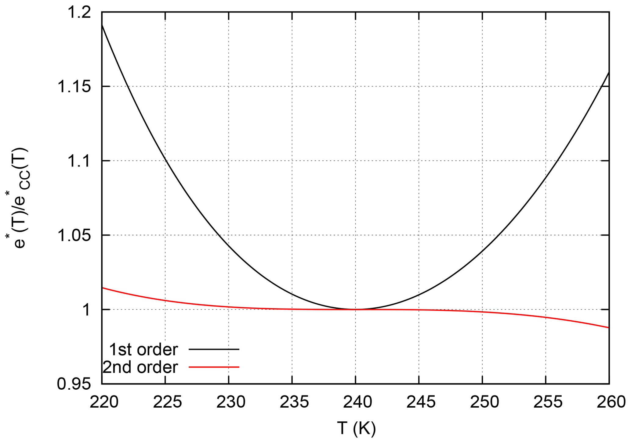
Figure 1 Ratio of the first-order (black) and second-order (red) approximations to the correct Clausius–Clapeyron saturation pressure of water vapour.

Also, the first-order approximation of the temperature dependence of the Planck function,

$$\begin{array}{}\text{(8)}& B_{\mathrm{1}}\left(T\right)=B\left(T_{\mathrm{0}}\right)\exp \left({\displaystyle \frac{hc}{\mathit{\lambda }k{T}_{\mathrm{0}}}}{\displaystyle \frac{T-T_{\mathrm{0}}}{T_{\mathrm{0}}}}\right)\end{array}$$

has relative errors of more than 10 % at low but not untypical upper-tropospheric temperatures; see Fig. 2. Thus we introduce a second-order approximation in the same way as above:

$$\begin{array}{}\text{(9)}& B_{\mathrm{2}}\left(T\right)=B\left(T_{\mathrm{0}}\right)\exp \left\{{\displaystyle \frac{hc}{\mathit{\lambda }k{T}_{\mathrm{0}}}}\left[{\displaystyle \frac{T-T_{\mathrm{0}}}{T_{\mathrm{0}}}}-{\left({\displaystyle \frac{T-T_{\mathrm{0}}}{T_{\mathrm{0}}}}\right)}^{\mathrm{2}}\right]\right\}.\end{array}$$

For this approximation the relative error does not exceed 3 % in the relevant temperature range, which suggests more accurate calculations of brightness temperature data.

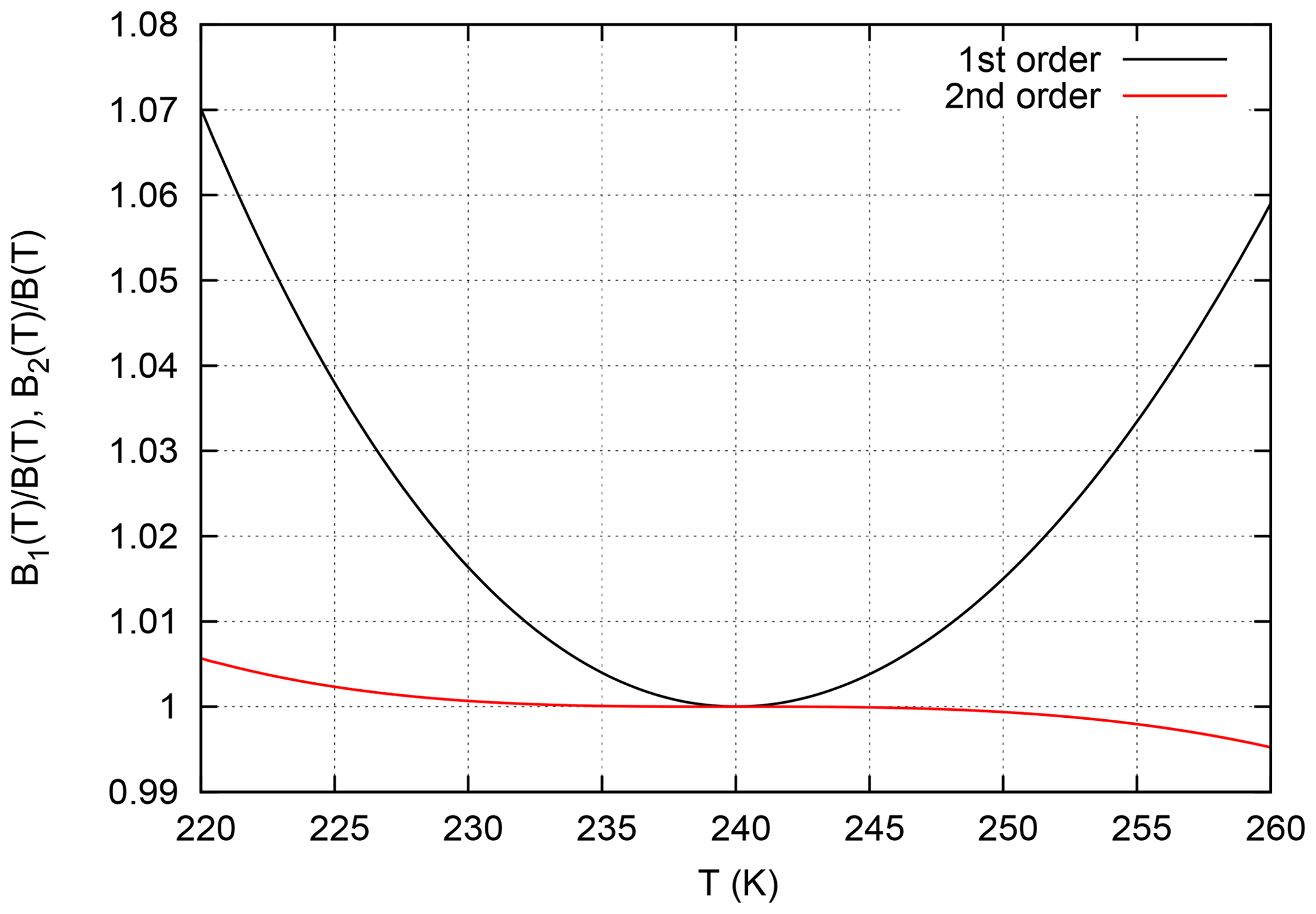
Figure 2 Ratio of first- (black) and second-order (red) approximations of the Planck function to the true Planck function vs. temperature, T. The wavelength for the calculation of the Planck functions was 6.7 µm.

3 Derivation of the second-order retrieval

3.1 Water vapour column density and optical depth

Let us now take the expression for the water vapour column density in Eq. (2) and invoke the mean value theorem for integration to draw the profile of relative humidity, r(p), outside the integral and write

$$\begin{array}{}\text{(10)}& w\left(p\right)={\displaystyle \frac{\mathit{ϵ}\stackrel{\mathrm{‾}}{r}\left(p\right)}{g}}\underset{\mathrm{0}}{\overset{p}{\int }}{\displaystyle \frac{e^{\ast }\left[T\right(p^{\prime }\left)\right]}{p^{\prime }}}\mathrm{d}{p}^{\prime }.\end{array}$$

$\stackrel{\mathrm{‾}}{r}\left(p\right)$ is a weighted mean relative humidity between the top of the atmosphere and pressure level p, defined as

$$\begin{array}{}\text{(11)}& \stackrel{\mathrm{‾}}{r}\left(p\right)={\displaystyle \frac{{\int }_{\mathrm{0}}^p\left[r\right(p^{\prime })/p^{\prime }]e^{\ast }\left[T\right(p^{\prime }\left)\right]\mathrm{d}{p}^{\prime }}{{\int }_{\mathrm{0}}^p[\mathrm{1}/p^{\prime }]e^{\ast }\left[T\right(p^{\prime }\left)\right]\mathrm{d}{p}^{\prime }}}.\end{array}$$

To proceed with the calculation of column density we need to calculate the integral

$$\begin{array}{}\text{(12)}& E^{\ast }\left(p\right)=\underset{\mathrm{0}}{\overset{p}{\int }}{\displaystyle \frac{e^{\ast }\left[T\right(p^{\prime }\left)\right]}{p^{\prime }}}\mathrm{d}{p}^{\prime }.\end{array}$$

The second-order approximation for the saturation pressure in pressure coordinates is

$$\begin{array}{}\text{(13)}& e^{\ast }\left(p\right)=e^{\ast }\left(p_{\mathrm{0}}\right)\exp \left[\mathit{\kappa }\mathit{\beta }\ln \left({\displaystyle \frac{p}{p_{\mathrm{0}}}}\right)-\mathit{\kappa }{\mathit{\beta }}^{\mathrm{2}}{\ln }^{\mathrm{2}}\left({\displaystyle \frac{p}{p_{\mathrm{0}}}}\right)\right],\end{array}$$

where we write p₀ for p(T₀). Substitution of x for ln (p∕p₀) gives the integral the following simple form:

$$\begin{array}{}\text{(14)}& E^{\ast }\left(p\right)=e^{\ast }\left(p_{\mathrm{0}}\right)\underset{-\mathrm{\infty }}{\overset{\ln (p/p_{\mathrm{0}})}{\int }}\exp (\mathit{\kappa }\mathit{\beta }x-\mathit{\kappa }{\mathit{\beta }}^{\mathrm{2}}{x}^{\mathrm{2}})\mathrm{d}x.\end{array}$$

The integral is of a form

$$\begin{array}{ll}{\displaystyle }\int & {\displaystyle }\exp [-(a{x}^{\mathrm{2}}+\mathrm{2}bx\left)\right]\mathrm{d}x={\displaystyle \frac{\mathrm{1}}{\mathrm{2}}}\sqrt{{\displaystyle \frac{\mathit{\pi }}{a}}}\exp \left({\displaystyle \frac{b^{\mathrm{2}}}{a}}\right)\\ \text{(15)}& {\displaystyle }& {\displaystyle }\text{erf}\left(\sqrt{a}x+{\displaystyle \frac{b}{\sqrt{a}}}\right)+\mathrm{const}\end{array}$$

(Abramowitz and Stegun, 1972, formula 7.4.32). Inserting the proper expressions for a:=κ β² and $b:=-\mathit{\kappa }\mathit{\beta }/\mathrm{2}$, we find

$$\begin{array}{ll}{\displaystyle }{E}^{\ast }\left(p\right)& {\displaystyle }={\displaystyle \frac{e^{\ast }\left(p_{\mathrm{0}}\right)}{\mathrm{2}\mathit{\beta }}}\sqrt{{\displaystyle \frac{\mathit{\pi }}{\mathit{\kappa }}}}\exp \left({\displaystyle \frac{\mathit{\kappa }}{\mathrm{4}}}\right)\\ \text{(16)}& {\displaystyle }& {\displaystyle }{\left[\text{erf}\left(\sqrt{\mathit{\kappa }}\mathit{\beta }x-\sqrt{\mathit{\kappa }}/\mathrm{2}\right)\right]}_{-\mathrm{\infty }}^{\ln (p/p_{\mathrm{0}})}{\displaystyle }& {\displaystyle }={\displaystyle \frac{e^{\ast }\left(p_{\mathrm{0}}\right)}{\mathrm{2}\mathit{\beta }}}\sqrt{{\displaystyle \frac{\mathit{\pi }}{\mathit{\kappa }}}}\exp \left({\displaystyle \frac{\mathit{\kappa }}{\mathrm{4}}}\right)\\ {\displaystyle }& {\displaystyle }\left[\text{erf}\left(\sqrt{\mathit{\kappa }}\mathit{\beta }\ln (p/p_{\mathrm{0}})-\sqrt{\mathit{\kappa }}/\mathrm{2}\right)+\mathrm{1}\right].\end{array}$$

Using this expression, and putting together all constant prefactors, the vapour column density above p is

$$\begin{array}{}\text{(17)}& w\left(p\right)=\mathrm{644.8}\cdot \stackrel{\mathrm{‾}}{r}\left(p\right)\left[\mathrm{1}+\text{erf}\left(\sqrt{\mathit{\kappa }}\mathit{\beta }\ln (p/p_{\mathrm{0}})-\sqrt{\mathit{\kappa }}/\mathrm{2}\right)\right]\end{array}$$

and the corresponding optical depth follows from Eq. (1). Note that the corresponding prefactor for the retrieval of UTHi is 847.9.

3.2 Radiance calculation

The radiance measured by the satellite instrument is given as the solution of the following simple form of the radiative transfer equation (see SB93 and SJW96):

$$\begin{array}{}\text{(18)}& I=\underset{\mathrm{0}}{\overset{\mathrm{\infty }}{\int }}\exp [-\mathit{\tau }(p\left)\right]{\displaystyle \frac{\mathrm{d}B\left(p\right)}{\mathrm{d}p}}\mathrm{d}p.\end{array}$$

The second-order formulation of the Planck function as a function of pressure is

$$\begin{array}{}\text{(19)}& B\left(p\right)=B_{\mathrm{0}}\exp \left[C_{\mathit{\lambda }}\mathit{\beta }\ln \left({\displaystyle \frac{p}{p_{\mathrm{0}}}}\right)-C_{\mathit{\lambda }}{\mathit{\beta }}^{\mathrm{2}}{\ln }^{\mathrm{2}}\left({\displaystyle \frac{p}{p_{\mathrm{0}}}}\right)\right],\end{array}$$

where we write B₀ for B(T₀) and where $C_{\mathit{\lambda }}=hc/\left(\mathit{\lambda }k{T}_{\mathrm{0}}\right)=\mathrm{8.95}$ is a constant, computed for a wavelength (λ) of 6.7 µm (and T₀=240 K). Further, we have

$$\begin{array}{}\text{(20)}& {\displaystyle \frac{\mathrm{d}B\left(p\right)}{\mathrm{d}p}}={\displaystyle \frac{B\left(p\right)C_{\mathit{\lambda }}\mathit{\beta }}{p}}\left[\mathrm{1}-\mathrm{2}\mathit{\beta }\ln \left({\displaystyle \frac{p}{p_{\mathrm{0}}}}\right)\right].\end{array}$$

We now introduce another abbreviation for use in the expression for the optical depth:

$$\begin{array}{ll}{\displaystyle }& {\displaystyle }{A}_{\mathit{\lambda }}=k_{\mathit{\lambda }}\sqrt{\mathrm{644.8}}\text{for UTH}\text{and}\\ \text{(21)}& {\displaystyle }& {\displaystyle }{A}_{\mathit{\lambda }}=k_{\mathit{\lambda }}\sqrt{\mathrm{847.9}}\text{for UTHi},\end{array}$$

and we replace $\stackrel{\mathrm{‾}}{r}\left(p\right)$ with a constant parameter U (or U_i) (the value of UTH or UTHi, whose meaning will be clarified later). Finally we substitute x for ln (p∕p₀). This gives

$$\begin{array}{ll}{\displaystyle }I=& {\displaystyle }{B}_{\mathrm{0}}{C}_{\mathit{\lambda }}\mathit{\beta }\underset{-\mathrm{\infty }}{\overset{\mathrm{\infty }}{\int }}\exp \left\{-A_{\mathit{\lambda }}\sqrt{U}{\left[\mathrm{1}+\text{erf}\left(\sqrt{\mathit{\kappa }}\mathit{\beta }x-\sqrt{\mathit{\kappa }}/\mathrm{2}\right)\right]}^{\mathrm{1}/\mathrm{2}}\right\}\\ \text{(22)}& {\displaystyle }& {\displaystyle }\exp \left[C_{\mathit{\lambda }}\right(\mathit{\beta }x-{\mathit{\beta }}^{\mathrm{2}}{x}^{\mathrm{2}}\left)\right](\mathrm{1}-\mathrm{2}\mathit{\beta }x)\mathrm{d}x.\end{array}$$

The integrand of this equation, which we will abbreviate as Φ(x;U) for later discussions, measures the contribution of each infinitesimal layer dx of the atmosphere to the flux of photons at the receiver. Dividing it by its integral gives a normalised weighting function – let us call it ϕ(x;U) – that has all properties of a probability density function in x with a form parameter U. This fact opens some interesting possibilities to compute moments, as for example the mean altitude from which photons emerge, its variance, the skewness of this distribution, etc. In the present paper we will not pursue these possibilities further.

For comparison we also show the first-order version that can be derived from Eq. (18) if we take the first-order formulation of the Planck function:

$$\begin{array}{ll}{\displaystyle }{I}_{\mathrm{1}}=& {\displaystyle }{B}_{\mathrm{0}}{C}_{\mathit{\lambda }}\mathit{\beta }\underset{-\mathrm{\infty }}{\overset{\mathrm{\infty }}{\int }}\exp \left(-A_{\mathit{\lambda }}^{\prime }\sqrt{U}{e}^{(\mathit{\beta }\mathit{\kappa }+\mathrm{1})x/\mathrm{2}}\right)\\ \text{(23)}& {\displaystyle }& {\displaystyle }\exp \left(C_{\mathit{\lambda }}\mathit{\beta }x\right)\mathrm{d}x,\end{array}$$

where $A_{\mathit{\lambda }}^{\prime }$ is an abbreviation for $k_{\mathit{\lambda }}\mathit{\left\{}\right(\mathit{ϵ}{e}^{\ast }\left(T_{\mathrm{0}}\right)p_{\mathrm{0}})/[g{p}_{\ast }(\mathit{\beta }\mathit{\kappa }+\mathrm{1})]{\mathit{\}}}^{\mathrm{1}/\mathrm{2}}$. Note that the same substitution has been made here as before for the sake of comparison. Using the logarithm is not actually necessary for the first order.

Figure 3 shows the two versions of the integrand just derived. The curves depend as expected on U, that is, higher U leads to lower integrals and thus lower radiances. The variation in the curves is similar in both panels, testifying to the correctness of the second-order calculations. In these integrands, U must be interpreted as that parameter that gives the resulting integral value, the radiance I, the correct (i.e. measured) value. The figure shows that for the same value of U, the radiances are higher in the second-order version than in first order.

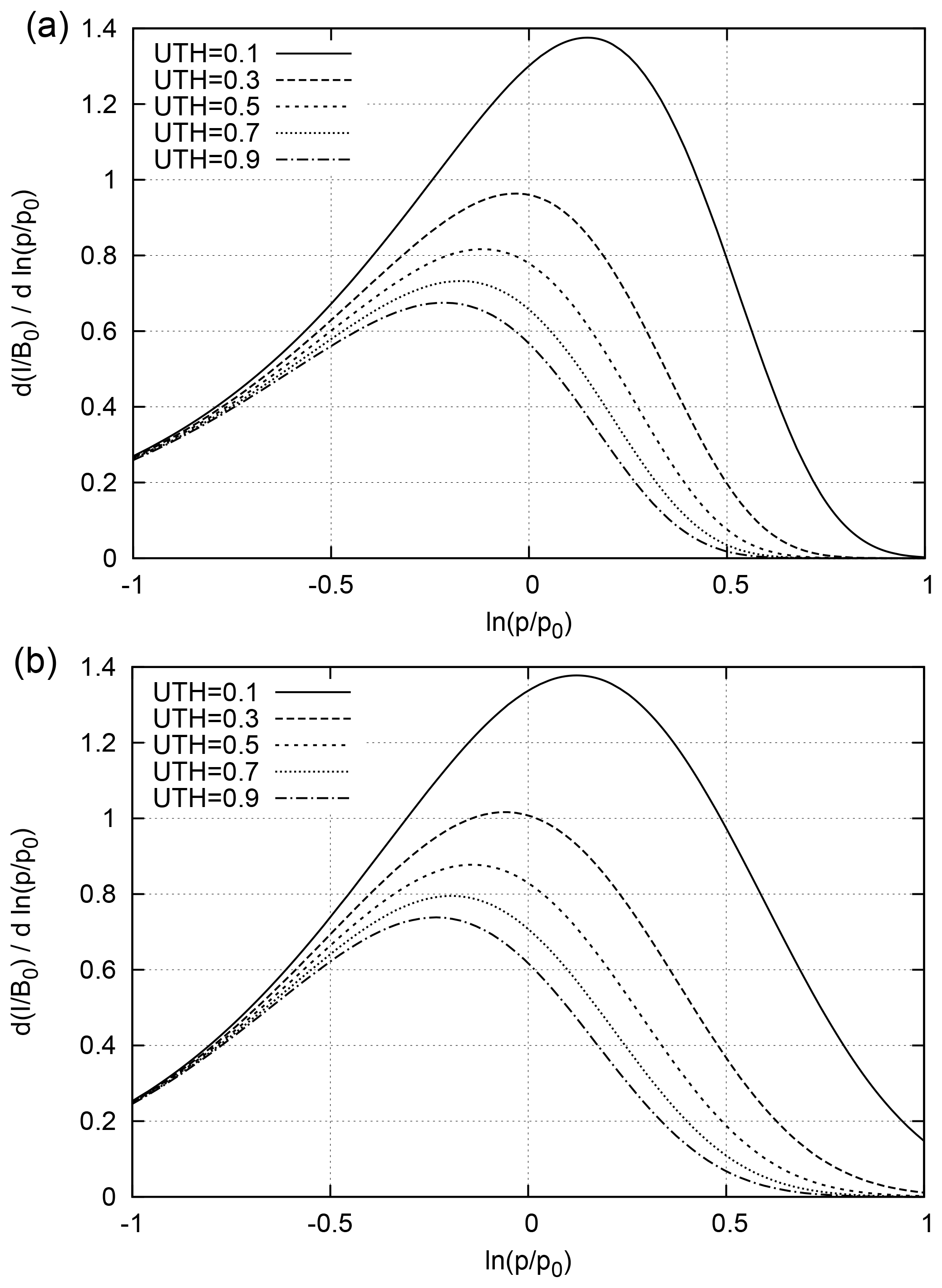
Figure 3 The function (normalised by the Planck function at T₀) to be integrated to get the radiance in channel 12 as a function of ln (p∕p₀) shown for various values of the UTH: (a) using the first-order approximations of SB93; (b) using the second-order approximations (this study). The higher the UTH, the less radiation is received at the satellite.

The necessary integrations were performed numerically (Romberg integration) and the results for UTH ranging from 1 % to 99 % are presented in Fig. 4 for the first- and second-order retrievals. As expected, the more humid the upper troposphere is, the lower the radiance at the satellite becomes. There is some radiation from altitudes below the 240 K level when the upper troposphere is quite dry, which explains the values above unity. For comparison and test purpose we have included the corresponding result of SB93, directly as given in that paper (labelled “analytically”, circles). This curve is practically identical to the numerically integrated one, which shows that the numerical integration works. The difference between the first- and second-order formulation turns out to be small but non-negligible.

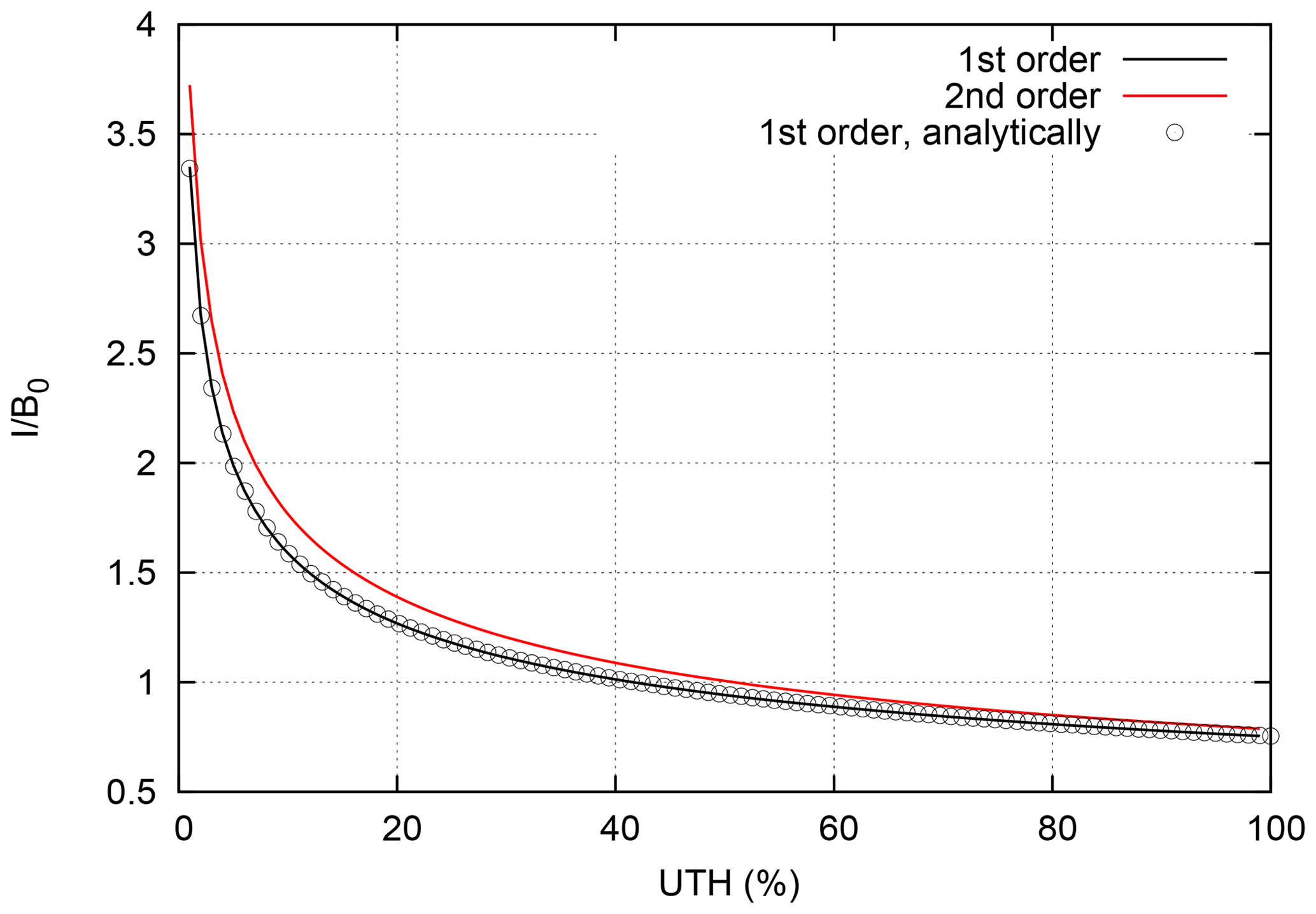
Figure 4 Normalised radiances, I∕B₀, resulting from numerical integration of Eqs. (22) and (23) for the first- (black) and second-order (red) retrievals. The curve consisting of circles is computed directly from the analytical formula (Eq. 18 of SB93).

Finally we need to express the radiances as brightness temperatures, T₁₂, where one can exploit the fact that 6.7 µm is on the Wien wing of the Planck function at T₀, that is,

$$\begin{array}{}\text{(24)}& {\displaystyle \frac{I}{B_{\mathrm{0}}}}={\displaystyle \frac{e^{hc/\mathit{\lambda }k{T}_{\mathrm{0}}}-\mathrm{1}}{e^{hc/\mathit{\lambda }k{T}_{\mathrm{12}}}-\mathrm{1}}}\approx \exp \left[{\displaystyle \frac{hc}{\mathit{\lambda }k{T}_{\mathrm{0}}}}\left(\mathrm{1}-{\displaystyle \frac{T_{\mathrm{0}}}{T_{\mathrm{12}}}}\right)\right].\end{array}$$

For the channel 12 brightness temperature, this gives the expression

$$\begin{array}{}\text{(25)}& T_{\mathrm{12}}={\displaystyle \frac{T_{\mathrm{0}}}{\mathrm{1}-\ln (I/B_{\mathrm{0}})/C_{\mathit{\lambda }}}},\end{array}$$

where I∕B₀ is a unique function of U. Four versions of the retrieval function are compared in Fig. 5, viz. the original function derived by SB93 (their Eq. 20, constants slightly adapted, that is, $e^{\ast }\left(T_{\mathrm{0}}\right)=\mathrm{37.7}$ Pa and μ=8.95, and their Eq. (23), which gives a slightly different result), the update of this function by Jackson and Bates (2001) without their correction for a variable lapse rate (i.e. the prefactor 1∕P_H they introduced is set to unity) and the new second-order retrieval. For the latter we have computed the integral of Eq. (22) for every integer value of U (1 % to 99 %), the radiance has been expressed as brightness temperature (Eq. 25) and the two resulting columns of data have been plotted against each other. The second-order retrieval gives higher UTH values than the other three retrievals at a given brightness temperature, except for temperatures below 240 K, where it matches the SB93 (their Eq. 23) line.

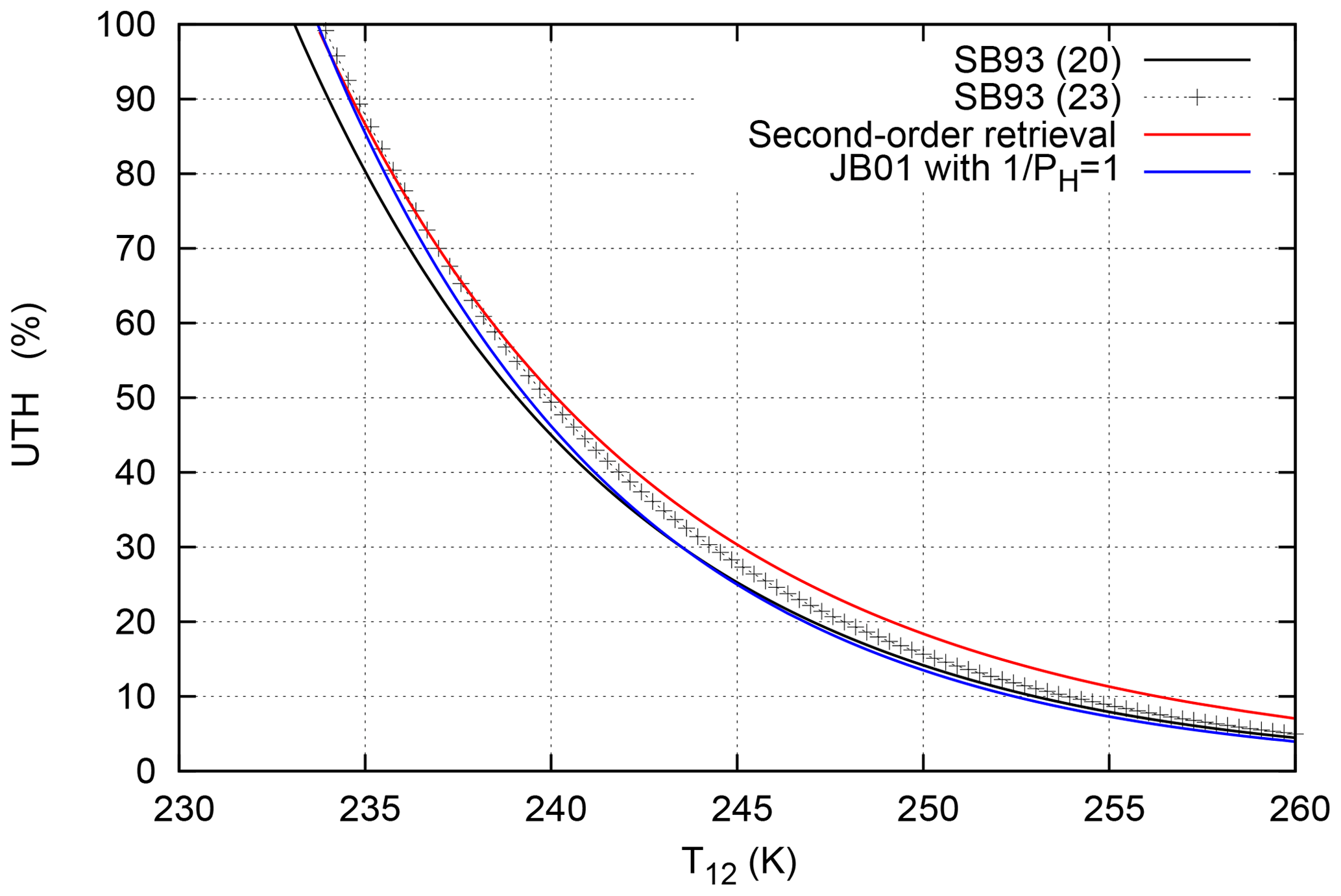
Figure 5 Comparison of retrieval functions UTH vs. T₁₂: the simple black line is the original function from SB93 (Eq. 20); the black line with crosses is their Eq. (23). The blue line is the improved SB93-type retrieval from JB01, shown here without the correction for lapse rate variability (i.e. $\mathrm{1}/P_H=\mathrm{1}$), and the red curve represents the second-order retrieval.

3.3 The retrieval for different channel central frequencies

The transition from HIRS/2 to HIRS/3 was accompanied by a change in the central wavelength of channel 12 from 6.7 to 6.5 µm (Shi and Bates, 2011). The spectroscopic quantities changed in a corresponding way. Furthermore, as we are interested in ice supersaturation, it is important to have the retrieval for UTHi as well, which implies a different saturation vapour pressure and a different factor κ. All necessary physical constants are given in Table 1 and the resulting retrieval functions are presented in Fig. 6.

Table 1 Constants used for the two different central wavelengths of HIRS channel 12 and fit coefficients.

Figure 6 Second-order retrieval functions for all cases of Table 1.

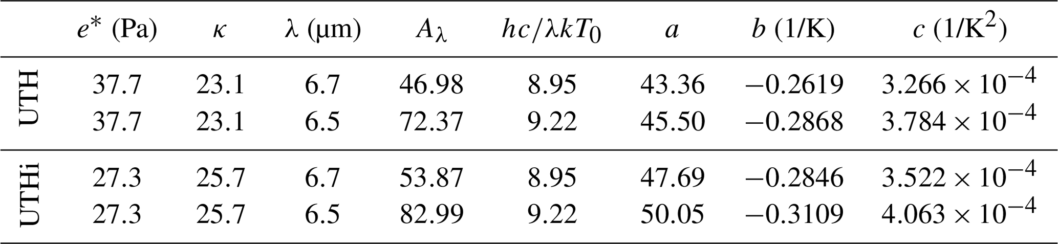
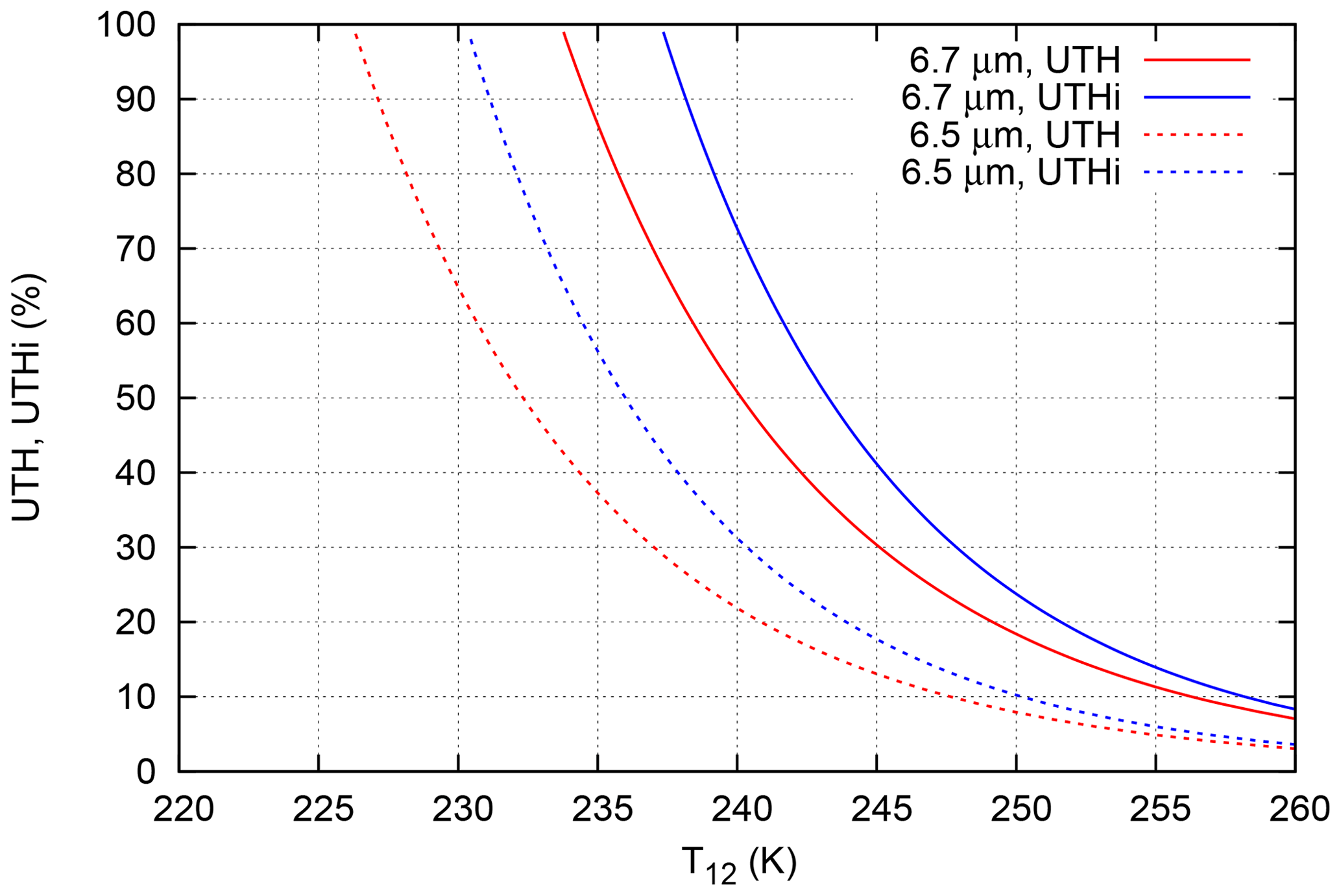
Since the atmosphere is more opaque at the latter wavelength, 6.5 µm, the HIRS/3 sensor is sensitive to a layer that is approximately 1 km higher than the layer HIRS/2 is sensitive to. The transition thus implies an average temperature change of −7 K (Gierens et al., 2018). This is reflected in the shift of the retrieval curves (compare the solid with the dotted UTH curves), the mean difference of which is very close to the expected 7 K. The same holds when comparing the solid and dotted UTHi curves. Therefore we expect that with the new second-order retrievals the number of ice-supersaturated cases from HIRS/2 and HIRS/3 and 4 sensors will become more similar than before. This expectation will be tested in the next section.

Table 1 contains three additional columns labelled $a,b,c$; these are fit coefficients computed with the Levenberg–Marquardt method (Press et al., 1989) that is implemented in gnuplot for the retrieval functions. The form of the fit is quite similar to the fit used by SB93 (Eq. 23), apart from the addition of a quadratic term that is appropriate for the second-order retrieval. Thus, for practical purpose one can use

$$\begin{array}{}\text{(26)}& U/\mathit{\%}=\mathrm{100}\exp \left(a+b{T}_{\mathrm{12}}+c{T}_{\mathrm{12}}^{\mathrm{2}}\right).\end{array}$$

It is not necessary to show the fits since they are nearly congruent with the retrieval functions.

Finally, we follow JB01 and introduce a prefactor that accounts for variability of the lapse rate factor β. Instead of repeating the derivation of the retrieval ab initio with variable β, JB01 introduced a correction that uses the brightness temperature measured with channel 6, T₆, and the final result is

$$\begin{array}{}\text{(27)}& U/\mathit{\%}=\mathrm{100}{\displaystyle \frac{\exp \left(a+b{T}_{\mathrm{12}}+c{T}_{\mathrm{12}}^{\mathrm{2}}\right)}{a^{\prime }+b^{\prime }{T}_{\mathrm{6}}}}.\end{array}$$

The coefficients $a^{\prime }=\mathrm{10.236}$ and $b^{\prime }=-\mathrm{0.036}$ have been recomputed by Gierens et al. (2014) in response to the change in the inter-calibration basis of the brightness temperatures between JB01 and Shi and Bates (2011).

4 Test applications

4.1 Application to computed brightness temperatures

While the jump in the mean retrieved brightness temperatures of channel 12 following the transition from HIRS/2 to HIRS/3 could be remedied with various methods (Shi and Bates, 2011; Gierens and Eleftheratos, 2017; Gierens et al., 2018), a pertinacious problem remained for cases with low brightness temperature (around 230 K and below) and corresponding high retrieved values of UTHi. We found that much more supersaturation (UTHi > 100 %) and high UTHi in general was retrieved from NOAA-15 than from NOAA-14 brightness temperatures of the same location and the same day (see, for instance, Fig. 1 of Gierens and Eleftheratos, 2017). Here we show that this problem no longer occurs when the second-order retrieval function for 6.7 µm is used for NOAA-14 and that for 6.5 µm is used for NOAA-15. Let us begin first with brightness temperatures derived from radiative transfer calculations for a large set of radiosonde profiles (meteorological observatory Lindenberg; see Gierens et al., 2018). Here we have two sets of brightness temperatures: one computed for the channel 12 spectral response function of NOAA-14 and one for NOAA-15. We now apply the UTHi fits of Table 1 and compare the resulting values. Figure 7 shows that the UTHi pairs from both retrievals are close to the diagonal line, and there is little deviation of the cloud of pairs from the diagonal at the upper end. So it seems that this old problem could be solved with the new retrieval.

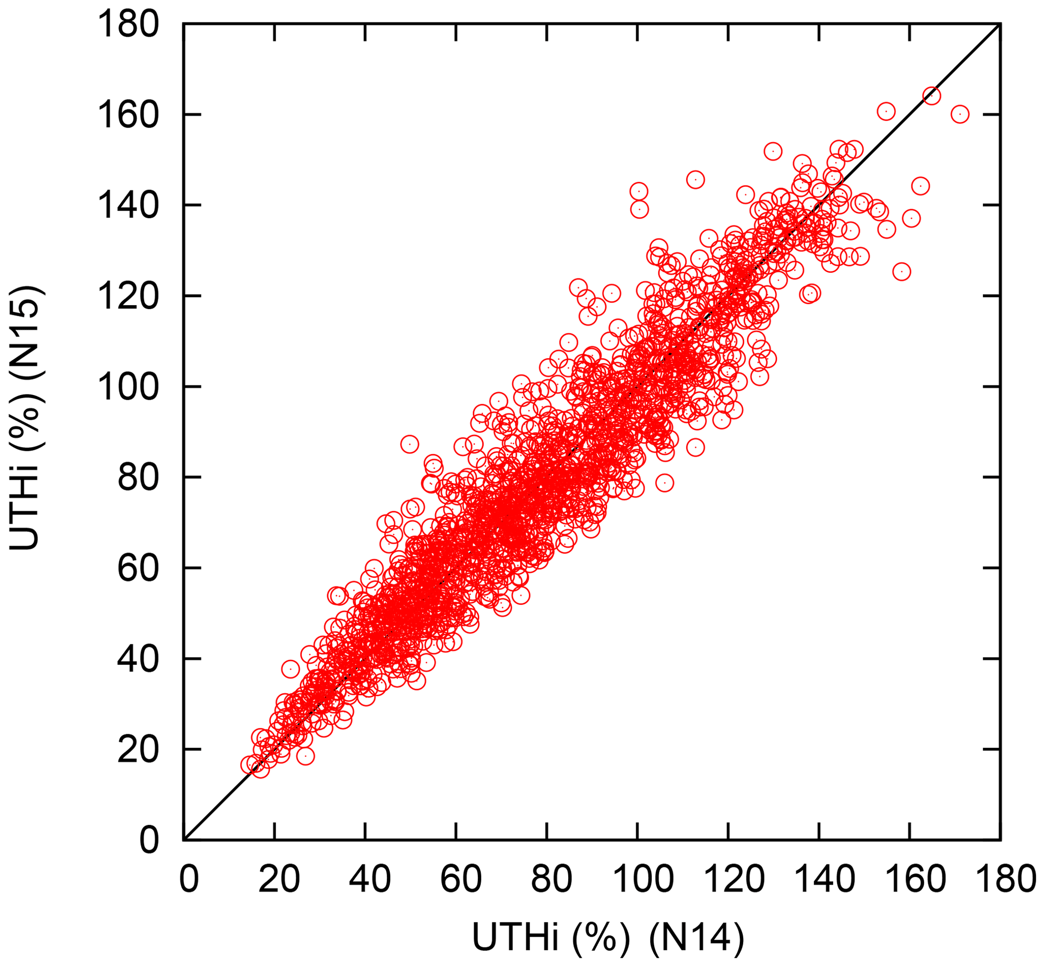
Figure 7 UTHi values from channel 12 brightness temperatures computed with a radiative transfer code using the NOAA-14 and NOAA-15 spectral response functions (Gierens et al., 2018). The UTHi values have been computed with the fit function given in the text using the coefficients from Table 1 for the two central wavelengths 6.7 (NOAA-14) and 6.5 µm (NOAA-15). The black line is simply the diagonal, and all points would ideally lie above it. Contrary to earlier inter-calibration attempts, the problem of having much more supersaturation cases in NOAA-15 than in NOAA-14 data is no longer present.

4.2 Application to the HIRS/2 to HIRS/3 transition

To check the performance of the second-order retrieval formulae on real brightness temperature data, we have used the clear-sky limb-corrected brightness temperatures measured by HIRS/2 on NOAA-14 and HIRS/3 on NOAA-15 on 1004 common days of operation. These data have been used in recent papers for similar checking purposes, for instance of the cdf (cumulative distribution function) nudging (Gierens and Eleftheratos, 2017) and the superposition methods (Gierens et al., 2018). To perform the check, the brightness temperatures are translated into UTHi according to the new formulation developed in this paper. Then UTHi is gridded on a 2.5^∘ × 2.5^∘ grid, and a daily average is formed for each grid point where data are available. A simple plausibility check removes all data where the corresponding UTH > 100 %. The valid daily averages are then compared day by day and grid by grid. This results in more than 700 000 data pairs, whose distribution is shown in Fig. 8. As the figure demonstrates, the data pairs are grouped along the diagonal line (black), and there is no deviation from this line towards the high UTHi values. The bivariate regression (red line) has the equation

$$\begin{array}{}\text{(28)}& U_i\left(\mathrm{N}\mathrm{15}\right)/\mathit{\%}=\mathrm{1.17}+\mathrm{0.998}{U}_i\left(\mathrm{N}\mathrm{14}\right)/\mathit{\%},\end{array}$$

with a slope of practically unity. The mean difference is −1.3 % and the standard deviation is 15.8 %.

With this result it can be expected that time series of high-UTHi cases can be constructed without the need for statistical corrections for the NOAA-14 and NOAA-15 T₁₂ data pairs. This will be considered next.

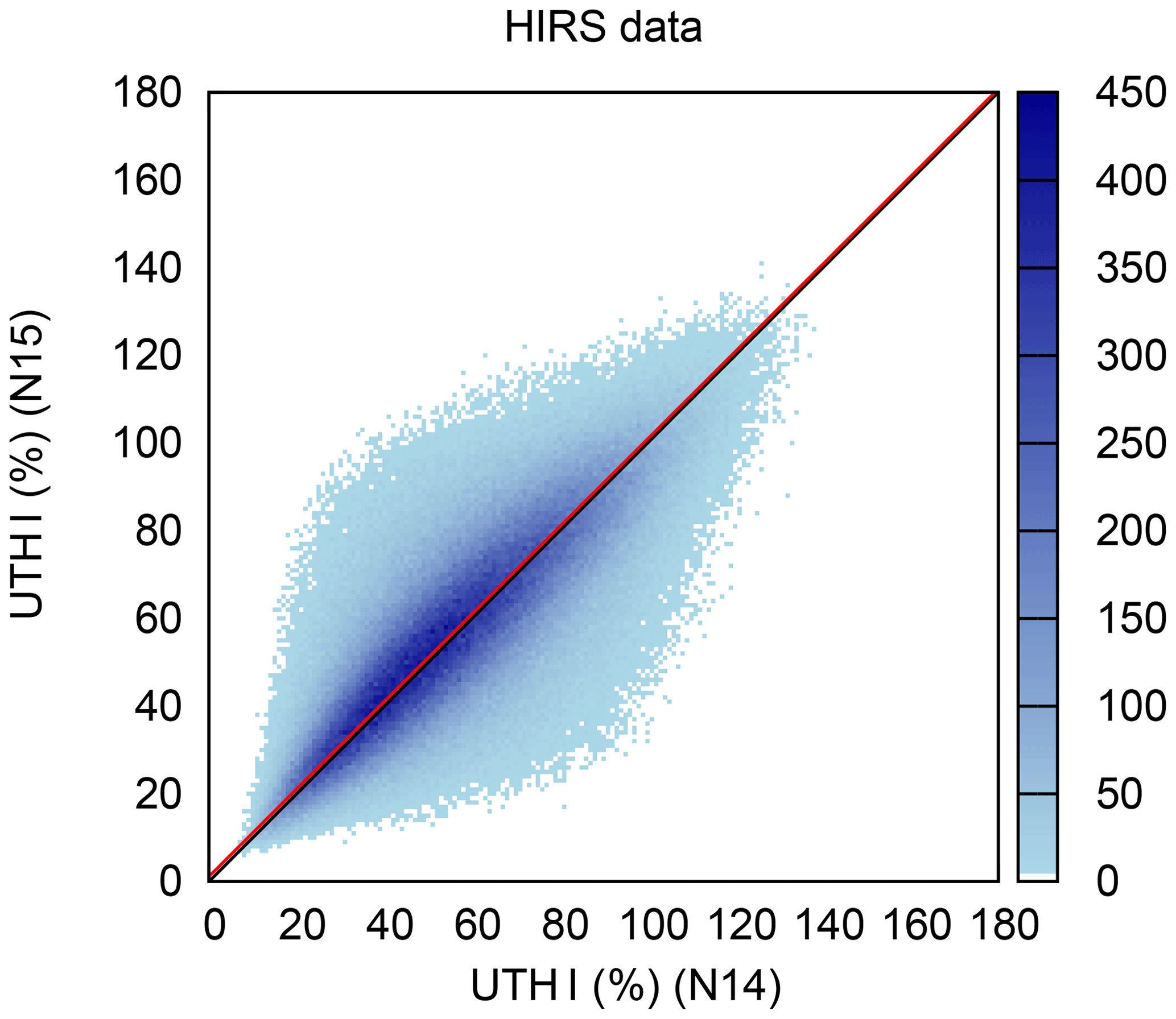
Figure 8 Heat map of UTHi from NOAA-15 vs. UTHi from NOAA-14 for 1004 common days of operation. The corresponding brightness temperatures have been transformed into UTHi using the second-order retrieval formulae derived in this paper. More details are given in the main text. Evidently the data pairs are nicely spread out along the diagonal line and there is not the same deviation from the diagonal in the upper UTHi range as before. The red line represents the bivariate regression between the two data sets. It is almost identical to the black diagonal.

4.3 Time series of occurrence of high UTHi cases

The above-mentioned problem of much higher cases of retrieved supersaturation after the HIRS/2 to HIRS/3 transition was first noticed by the authors when we made Fig. 9a in (Gierens and Eleftheratos, 2017); hereafter abbreviated GE17. That figure was produced using the inter-calibrated data of Shi and Bates (2011) and showed a very steep increase in the occurrence frequency of high UTHi (>70 %) cases, and the time when the increase started coincided with the start of NOAA-15 and the corresponding transition to a new channel 12 central frequency. Figure 9 shows the time series of high UTHi-value occurrences from July 1979 to December 2014 computed from non-inter-calibrated HIRS data (monthly frequencies of daily mean values per 2.5^∘ × 2.5^∘ grid box in the midlatitude zone 30 to 70^∘ N) using the second-order retrieval for 6.7 µm up to NOAA-14 and for 6.5 µm from NOAA-15 on. The figure shows a tendency for increasing frequencies as well, but it is a small increase instead of a nearly exponential one as seen in Fig. 9a of GE17. One can also notice a minimum after 1985 followed by quite a strong increase just before 1990.

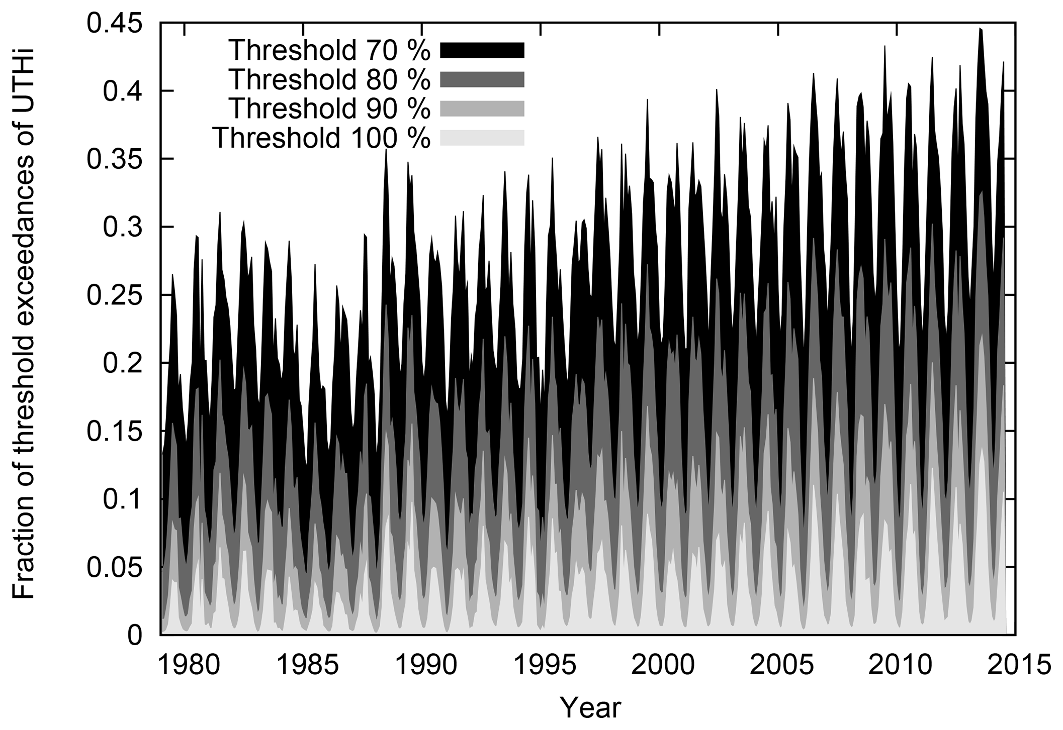
Figure 9 Time series of monthly fractional threshold exceedances for UTHi exceeding 70 %, 80 %, 90 % and 100 % (various grey scales) in the Northern Hemisphere between 30 and 70^∘ N and from July 1979 to December 2014.

For a more detailed study of these time series it would be better to have the series NOAA-6 to NOAA-14 and the subsequent one NOAA-15 to MetOp 2 inter-calibrated instead of using non-inter-calibrated data. For this it seems possible to use the channel 12 and 6 data inter-calibrated to NOAA-12 (Shi and Bates, 2011; Gierens et al., 2014) for NOAA-6 to NOAA-14 and the data that are inter-calibrated to Metop-A (Shi and Bates, 2011) for NOAA-15 and later satellites. An inter-calibration between NOAA-14 and NOAA-15 should, however, be replaced by using different retrieval formulae as done here.

4.4 The probability distribution of UTHi

The same daily values as before can be used to determine the probability distribution of UTHi. We have done this for the second-order retrieval with the non-inter-calibrated data as above, but for the JB01 retrieval it was necessary to use the inter-calibrated data.

Figure 10 shows probability density functions of UTHi in both versions of the retrieval and for different periods of time. Solid curves represent data from 1979 to 2014; the dashed and dotted curves represent the earliest and latest approximately 10 years in our data set 1979–1989 and 2006–2014, respectively. Recall that in the first of these periods the satellites carried HIRS/2 only and in the last period only HIRS/3 or HIRS/4. There is no qualitative difference between the curves of the different time periods and HIRS versions. All curves have a similar shape, but with the second-order retrieval the pdf (probability density function) has a longer tail to high and supersaturated values, as can be expected from the foregoing discussion. The upper tail is exponentially distributed in all pdfs shown. An exponential distribution of supersaturation values is expected from many other data sets studied (e.g. aircraft in situ measurements, radiosondes, other satellites: Gierens et al., 1999; Spichtinger et al., 2002, 2003; Haag et al., 2003; Gettelman et al., 2006; Lamquin et al., 2009).

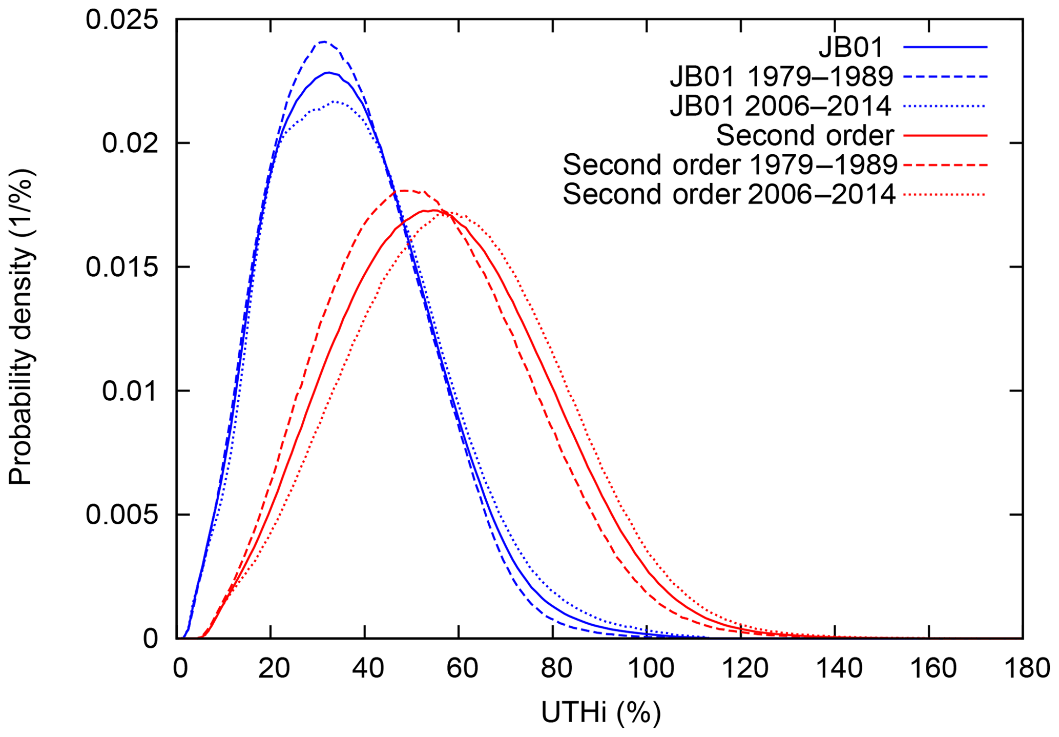
Figure 10 Probability density functions of UTHi retrieved with the formula of JB01 (using inter-calibrated brightness temperatures, blue) and with the second-order retrieval (using non-inter-calibrated brightness temperatures, red). Solid curves represent data from 1979 to 2014; dashed: data from 1979 to 1989; dotted: data from 2006 to 2014. We note that all curves have a similar shape but with the second-order retrieval, the pdf has a longer tail to high and supersaturated values. The upper tail is exponentially distributed in all pdfs shown. In both retrievals, the data show a tendency to higher UTHi values over the long observation period.

Mean values ± 1 standard deviation for the pdfs are as follows for the JB01 data: 37.2±16.7 % for the overall data set, 36.2±15.8 % for the period 1979–1989 and 38.5±17.6 % for 2006–2014. The corresponding values for the second-order retrieval are 56.8±21.9 % for all data, 53.6±21.2 % for 1979–1989 and 59.7±22.6 % for 2006–2014. In both retrievals, the data show a tendency to higher UTHi and fewer low values over the long observation period, which is consistent with the increasing tendency that can also be seen in Fig. 9. Also, the distributions become slightly broader. It should be noted that the pdfs and their trends refer to clear sky only, since the data have been cloud-cleared by Shi and Bates (2011) using the cloud-clearing procedure detailed by Jackson et al. (2003).

An obvious question is whether this trend of increasing UTHi is true or an artefact. For instance, an increase in thin high cirrus clouds or contrail cirrus (thin enough to stay undetected by the applied cloud-clearance methods) would lead to lower brightness temperatures and thus higher retrieved UTHi values. However, studies of cirrus occurrence (e.g. by Minnis et al., 2004; Eleftheratos et al., 2007) indicate declining cirrus coverage at many locations of the world, and only where air traffic is intense, is the declining trend balanced by increasing contrail cover. Now, there is a decadal increase in UTHi over Siberia and a slight decrease over the western North Atlantic (Gierens et al., 2014, their Fig. 3), which is hardly explainable with air traffic patterns in these two regions. It also hardly conceivable that orbital drifts of the satellites could reflect any significant trend, which would need a single satellite with a drift and a diurnal cycle of relative humidity in the UT that is stable over the whole observation period. However, there are many satellites, generally with overlapping operation and in morning and afternoon orbits, such that any single pseudo-trend would become averaged out. In addition, recall that the time series presented in Fig. 9 comes from monthly means of daily means averaged over quite a wide latitude zone (30–70 ^∘N), and as such, it is hardly possible that any daily orbital drift could determine the behaviour of the monthly zonal mean. Another potential contribution to the positive trend may come from the global increase in the concentration of carbon dioxide (CO₂). Using radiative transfer calculations, Shi et al. (2016) showed that an increase in the CO₂ concentration from 330 to 410 ppmv leads on average to a decrease in T₆ by about 2 K. Gierens et al. (2014, their Fig. 7) found that T₆ was up to 1 K lower in the 1980s than in 2000–2009 (in the northern midlatitudes). According to Eq. (27), a decrease in T₆ contributes to an increase in UTHi, but the contribution is about 5 times smaller than the contribution from changes in T₁₂ (Gierens et al., 2014, Appendix A). Finally, we want to mention that global climate models consistently show increases in relative humidity in the extratropical upper troposphere (e.g. Sherwood et al., 2010; Wright et al., 2010; Irvine and Shine, 2015).

5 On the meaning and purpose of UTH

5.1 Simple postulates

When we are talking about upper-tropospheric humidity we must distinguish the substance water vapour in the upper troposphere from the physical quantity UTH. While the substance is clearly defined and can be seen nicely, for instance on satellite images in the water vapour channels, the definition of the physical quantity UTH is not necessarily unique. If humidity and temperature profiles are given in high resolution, UTH can be defined as a weighted mean over the humidity profile where the weighting function is given by the transfer of radiation through the atmosphere. Evidently, the definition then depends on radiation details (e.g. wavelength, channel width, filter function). In practice, however, we do not know the necessary profiles. All that is given is the brightness temperature measured by channel 12, and U is simply a function of T₁₂. That there is no UTH per se and thus no true value implies that there is no wrong value either. Hence the function that maps T₁₂ into U is in principle arbitrary. Is it then possible to validate an UTH algorithm? Now, validation is often mistaken for verification, and this makes no sense when there is no truth. Validation, in the sense of Oreskes et al. (1994), means the “establishment of legitimacy”, which has connotations of usefulness. Certainly there are more or less useful mappings from T₁₂ into U when the interest is a typical or “mean” relative humidity in the upper troposphere. To be a useful quantity, UTH as determined from the brightness temperature should obey a number of postulates.

A simple postulate is that UTH should have values on the familiar scale of relative humidity: that is, 0 % $<U<\mathrm{100}$ % and 0 % < U_i, where the latter can exceed 100 %, like relative humidity with respect to ice does. This is usually fulfilled, and values U>100 % are discarded as bad data.

An increase in relative humidity somewhere in the region to which HIRS channel 12 is sensitive should result in increasing UTH. This postulate is fulfilled if the temperature decreases upwards in the layers where the weighting function has non-negligible values. A temperature inversion in that layer would violate the basic assumptions for the retrieval and thus yield bad results (cf. the warning expressed by SB93, after their Eq. 16).

Another simple postulate that is important for consistency is that in an academic case of a constant relative humidity throughout the atmosphere, say r(p)=r₀, U should have the same value, that is, U=r₀. This postulate is not generally fulfilled when in the defining integral for w(p) the factor r(p)∕p is drawn out instead of only r(p). The original derivation of SB93 is equivalent to drawing out r(p)∕p of the integral. p is replaced by the constant p_∗. This leads to

$$\begin{array}{}\text{(29)}& \stackrel{\mathrm{‾}}{r}\left(p\right)=p_{\ast }{\displaystyle \frac{{\int }_{\mathrm{0}}^p\left[r\right(p^{\prime })/p^{\prime }]e^{\ast }\left[T\right(p^{\prime }\left)\right]\mathrm{d}{p}^{\prime }}{{\int }_{\mathrm{0}}^p{e}^{\ast }\left[T\right(p^{\prime }\left)\right]\mathrm{d}{p}^{\prime }}},\end{array}$$

and the two integrals do not cancel if r(p)=r₀, and in general $\stackrel{\mathrm{‾}}{r}\left(p\right)\ne r_{\mathrm{0}}$. Thus, the consistency postulate is not fulfilled in that case. In contrast, in the approach by SJW96, only r(p) is drawn out, and the two integrals (Eq. 11) cancel if r(p)=r₀ such that $\stackrel{\mathrm{‾}}{r}\left(p\right)=r_{\mathrm{0}}$. We followed their method in our derivation.

Furthermore, the ratio U_i∕U should depend on the brightness temperature of the water vapour channel in a way similar to the dependence of r_i∕r on local temperature. This is considered next in some detail.

5.2 The relation between UTH and UTHi

Between the local quantities r(p) and r_i(p) (relative humidity with respect to supercooled liquid water and ice, respectively), the relation $r{e}_w^{\ast }\left(T\right)=r_i{e}_i^{\ast }\left(T\right)$ holds. A similar relation should hold between U and U_i. Figure 11 shows a number of curves. The solid black one is the ratio between the saturation vapour pressures as a function of temperature (using the formulas of Murphy and Koop, 2005) that holds locally (at a point). The dashed black curve is the corresponding non-local ratio $E_w^{\ast }\left(T\right)/E_i^{\ast }\left(T\right)$. Using the fit coefficients from Table 1 and Eq. (26), we compute U_i∕U for the two wavelengths as functions of temperature (red lines). The blue line is the corresponding ratio using the coefficients from JB01. The black rectangle in the middle represents the range of values we computed from over 1600 radiosonde profiles of Lindenberg (using Eq. 10 with the 245 K isotherm as the lower integration limit and Eq. (5) for the representation of the vapour pressure). Evidently, the new second-order retrieval leads to U_i∕U values that obey the postulation that such ratios should be close to $E_w^{\ast }\left(T\right)/E_i^{\ast }\left(T\right)$. U_i∕U in the version of JB01 is far below the reference.

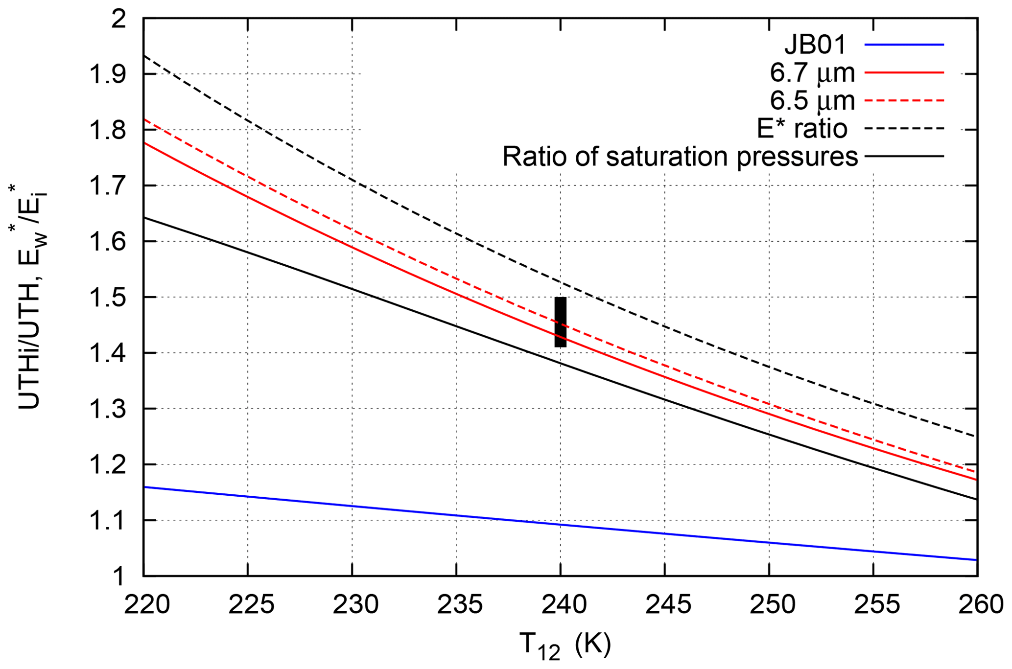
Figure 11 Ratio of UTHi vs. UTH retrieval (blue: JB01; red: present paper using the retrieval for 6.7 µm (solid) and the same but for the 6.5 µm retrieval (dashed)) as a function of brightness temperature. The other curves are for comparison. The black solid line is the ratio of saturation vapour pressures $e_w^{\ast }\left(T\right)/e_i^{\ast }\left(T\right)$ (Murphy and Koop, 2005), and the black dashed line represents the ratio of the corresponding $E_{w/i}^{\ast }\left(T\right)$ functions (Eq. 16 with the corresponding parameters from Table 1). The black bar in the middle represents more than 1600 values computed by integration over the actual RH, RH with respect to ice and T profiles from the Lindenberg radiosoundings, assuming the lower integration limit is 245 K (Eq. 10). Obviously, the second-order formula matches the actual data quite well, but the ratio obtained from the JB01 coefficients is quite different.

This fact explains why the frequency values (y axis) in Fig. 9 are much larger than in our previous paper (GE17). In that paper we used the JB01 formulation, and this seems to underestimate U_i when it computes U correctly (as Fig. 5 shows, the JB01 retrieval of UTH is consistent with the second-order retrieval). Thus it seems that we have underestimated the frequency of high-U_i cases in previous papers, and the new formulation will give more reliable results.

We note, however, two subtle issues. First, the retrieved U_i∕U ratio depends on the channel wavelength, which is surprising. The source of the difference lies in the non-locality of this ratio and the fact that 6.7 and 6.5 µm photons originate from different layers. The second issue is that U_i∕U is not exactly $E_w^{\ast }\left(T\right)/E_i^{\ast }\left(T\right)$. This is because the assumed structure of the atmosphere depends a little on whether it is modelled via the relative humidity over liquid water or via the relative humidity over ice. This small difference arises because of the approximation of the saturation vapour pressure formulation. So, in Eq. (22) the optical thickness is differently distributed as a function of pressure altitude when we use r_i and the corresponding quantities instead of r. Fortunately, these differences and issues are small.

5.3 Comparison to regression approach

Traditionally the coefficients in the retrieval formula are determined via a regression process, based on a large number of humidity and temperature profiles (e.g. Jackson and Bates, 2001). In order to obtain the necessary average over the profile of relative humidity, a weighting function is applied. There is some freedom in choosing the weighting function; thus several possibilities have been tested and the one resulting in the lowest scatter is selected (Jackson and Bates, 2001; Brogniez et al., 2009; Schröder et al., 2014). The relative humidity profile weighted with the optimal weighting function is integrated and then taken as the upper-tropospheric humidity (or free-tropospheric humidity). It should be noted that the weighting function in this method is computed with full radiative transfer and actual atmospheric profiles, while the retrieval formula to which the regression coefficients are applied is based on the first-order simplifications mentioned above. This is a subtle inconsistency that has to our knowledge not been noticed before.

Our approach does not involve a regression to determine the coefficients. As described in Sect. 3.3, they follow from a numerical fit to the theoretically derived functions shown in Fig. 6. The upper-tropospheric humidity in our case is that value that must be inserted into Φ(x;U) in order to fulfill Eq. (22). It is evident that this approach involves a different kind of weighting of the humidity profile than the traditional methods described in the studies mentioned.

Now assume a profile r(x) of relative humidity is given without accompanying satellite information on T₁₂, but one is interested in the value of UTH, for instance for diagnostic purpose. The result should be consistent with the retrieved UTH that would be determined if the corresponding brightness temperature were available. What can be done? It is possible to run a radiative transfer code to calculate the channel 12 brightness temperature and then to apply one of the retrieval methods to get the UTH. Another possibility from the radiative transfer code is to obtain the weighting functions mentioned above and then to compute the UTH as the correspondingly weighted average of r(x). These two answers will generally differ because of the inconsistency mentioned above.

5.4 The ill-posedness of the problem and interpretation of UTH

Nothing demonstrates the ill-posedness of the problem to determine a typical relative humidity of the upper troposphere from just one datum, the measured brightness temperature, better than Eq. (22). On the left side of the equation there is the given radiance (measured or computed with a radiative transfer model) which one tries to reproduce with an appropriate choice of U in the function Φ. Now, while I (or T₁₂) is the result of a full radiative transfer through the real atmosphere, Φ represents a simplified radiative transfer through a pseudo-atmosphere. One must conclude that U is the mean UTH in such a simple atmosphere with simple radiation physics that would yield the same radiance as the true measured one.

Furthermore, Eq. (22) is not the only possibility for a simplified radiative transfer in a pseudo-atmosphere. Equation (23) shows an example of the first-order approximations. Evidently, using Eq. (23) instead of Eq. (22) requires a different U to reproduce the measured radiance. But this is still not the end of the story; the operator Φ(x;U) can represent any model atmosphere and any more or less sophisticated radiative transfer. This combination determines the resulting U. In this spirit it is possible to obtain an optimal U if actual profiles of r(p) and T(p) are given and if Φ(x;U) represents a full radiative transfer through the actual atmosphere. In this case, Φ should be written as $\mathrm{\Phi }[p;r(p),T(p\left)\right]$ to make the dependencies clear.

It is evident that UTH (and UTHi) does not only represent the humidity in the upper troposphere and the radiation transfer as such. It also represents the kind of model atmosphere and the kind of radiative transfer model that is used to define the operator Φ.

6 Conclusions

In spite of the largely successful inter-calibration of the HIRS channel 12 data (Shi and Bates, 2011), which works well for the bulk of the data, there remained a pertinacious problem in the high range of upper-tropospheric humidities retrieved from the inter-calibrated brightness temperatures: the change in channel wavelength from 6.7 to 6.5 µm, where the atmosphere is more opaque, resulted in quite a strong increase in the frequency of high and very high values of UTHi. Over the last years we tried different potential remedies (adjustment of low brightness temperatures using so-called cdf nudging and the additional use of channel 11 brightness temperatures), but these were not completely satisfying. Gierens et al. (2018) speculated that the linearisations used in the derivation of the original retrievals by SB93 and SJW96 were insufficient for the tails of the UTH and UTHi distributions and we hoped that a retrieval with second-order approximations would yield better results. In reworking the derivation we noticed the necessity to adapt the optical constant k_λ to the changed channel wavelength, and it turned out that this adaptation is the key to the desired smooth transition from HIRS/2 to HIRS/3, that is a transition without a jump in the frequency of high UTHi values.

The achievements of this paper are as follows:

1. The second-order approximations give a more accurate representation of the variation in water vapour saturation pressure and the Planck function with temperature in the relevant range of T than linearisations.

2. The change in k_λ reflects the change in wavelength and leads to a smooth HIRS/2 to HIRS/3 transition. Comparing data from 1004 days of common operation of NOAA-14 and NOAA-15 leads to a scatter plot of pairs of UTHi values that has a bivariate regression function with a slope of nearly unity and a small intercept.

3. For future applications we provide retrieval coefficients for both UTH and UTHi and for both HIRS/2 and HIRS/3/4. The mathematical form of the retrieval formula is similar to that given by JB01 but includes the second order of T₁₂ under the exponential function.

4. A first application of the new method indicates a moistening of the upper troposphere (in northern midlatitudes) over the last decades, consistent with earlier results (Soden et al., 2005; Gierens et al., 2014).

5. We argue that our method fulfills a set of consistency requirements (postulates).

The second-order retrieval has been used to produce UTHi data for the northern midlatitudes. The same retrieval will be applied to produce UTHi data for the tropics (30^∘ N to 30^∘ S) and the southern midlatitudes (30 to 70^∘ S). A near-global UTHi satellite data set will allow us to investigate the natural variability of UTHi on larger space scales. We need to know whether natural cycles or other events (e.g. seasonal variations, quasi-biennial oscillation, El Niño–Southern Oscillation, North Atlantic Oscillation, solar cycle) have an imprint on UTHi that can be detected in the data after the application of our retrieval, and we need to understand to what degree these natural fluctuations affect the natural variability of UTHi. With this long-term data set of 35+ years, we are particularly interested in exploring trends in the mean and in high UTHi values, which are important to follow the evolution of cirrus cloudiness in a future warmer climate. The studies are going to be performed using a time series that is composed of two inter-calibrated data sets (one for HIRS/2 only and one for HIRS/3 and 4) and one without an inter-calibration between NOAA-14 and 15 as has been done here.