Characterization of ozone production in San Antonio, Texas, using measurements of total peroxy radicals

Observations of total peroxy radical concentrations ([XO₂] ≡ [RO₂] + [HO₂]) made by the Ethane CHemical AMPlifier (ECHAMP) and concomitant observations of additional trace gases made on board the Aerodyne Mobile Laboratory (AML) during May 2017 were used to characterize ozone production at three sites in the San Antonio, Texas, region. Median daytime [O₃] was 48 ppbv at the site downwind of central San Antonio. Higher concentrations of NO and XO₂ at the downwind site also led to median daytime ozone production rates (P(O₃)) of 4.2 ppbv h⁻¹, a factor of 2 higher than at the two upwind sites. The 95th percentile of P(O₃) at the upwind site was 15.1 ppbv h⁻¹, significantly lower than values observed in Houston. In situ observations, as well as satellite retrievals of HCHO and NO₂, suggest that the region was predominantly NO_x-limited. Only approximately 20 % of observations were in the VOC-limited regime, predominantly before 11:00 EST, when ozone production was low. Biogenic volatile organic compounds (VOCs) comprised 55 % of total OH reactivity at the downwind site, with alkanes and non-biogenic alkenes responsible for less than 10 % of total OH reactivity in the afternoon, when ozone production was highest. To control ozone formation rates at the three study sites effectively, policy efforts should be directed at reducing NO_x emissions. Observations in the urban center of San Antonio are needed to determine whether this policy is true for the entire region.

1 Introduction

Tropospheric ozone (O₃) is a secondary air pollutant formed through a series of reactions involving volatile organic compounds (VOCs) and NO_x ([NO_x] ≡ [NO] + [NO₂], where NO is nitric oxide and NO₂ is nitrogen dioxide). While tropospheric ozone exists naturally through stratospheric transport (Holton et al., 1995) and in situ tropospheric production, human activities have drastically perturbed these background values (Lamarque et al., 2005). Exposure to ozone adversely impacts human health, limiting lung and cardiac function, exacerbating chronic respiratory illnesses, and precipitating early mortality (Bell et al., 2006; Park et al., 2005; Jerrett et al., 2009; Silva et al., 2013). In response to these adverse impacts, in 2015 the United States Environmental Protection Agency (EPA) imposed an 8 h ozone standard of 70 ppbv, lowering the exposure limit from the 75 ppbv standard set in 2008 (EPA, 2015). While ambient concentrations of the ozone precursor NO_x have declined significantly over much of the US (Choi and Souri, 2015; He et al., 2013; Duncan et al., 2016; Lamsal et al., 2015), reductions in ozone concentrations have been less dramatic. Background ozone concentrations have actually increased in some locations (Cooper et al., 2012; Choi and Souri, 2015); in other areas that have seen decreases in ambient ozone concentrations, such as Texas and the Mid-Atlantic region, ozone still periodically exceeds the EPA standard (e.g., He et al., 2013).

Ozone production is generally classified as either NO_x- or VOC-limited (Kleinman, 1994; Thornton, 2002). Net formation of ozone occurs when NO is oxidized to NO₂ by reaction with the hydroperoxyl radical (HO₂) or an organic peroxy radical (RO₂). In the NO_x-limited regime, comparatively low concentrations of NO_x allow for the removal of RO_x radicals ([RO_x] ≡ [OH] + [HO₂] + [RO₂], where OH is the hydroxyl radical) through self-reactions (e.g., Reactions R1–R3). In the VOC-limited regime, RO_x radicals are removed from the atmosphere via reactions with NO_x, producing less reactive compounds such as nitric acid (HNO₃) (Reactions R4–R6). In the NO_x-limited regime, reductions in NO_x lead to reductions in O₃, while in the VOC-limited regime, reductions in NO_x without concomitant reductions in VOCs can actually increase O₃ production. One prominent example of this is the weekday–weekend effect in the southern California South Coast Air Basin, where O₃ increases on weekends due to decreases in NO_x emissions from heavy-duty diesel trucks (Pollack et al., 2012). The effective implementation of ozone reduction policies therefore requires a detailed understanding of the ozone production regime of the target area.

$$\begin{array}{}\text{(R1)}& {\displaystyle }& {\displaystyle }{\mathrm{HO}}_{\mathrm{2}}+\mathrm{OH}\to {\mathrm{H}}_{\mathrm{2}}\mathrm{O}+{\mathrm{O}}_{\mathrm{2}}\text{(R2)}& {\displaystyle }& {\displaystyle }{\mathrm{HO}}_{\mathrm{2}}+{\mathrm{HO}}_{\mathrm{2}}+\mathrm{M}\to {\mathrm{H}}_{\mathrm{2}}{\mathrm{O}}_{\mathrm{2}}+{\mathrm{O}}_{\mathrm{2}}+\mathrm{M}\text{(R3)}& {\displaystyle }& {\displaystyle }{\mathrm{HO}}_{\mathrm{2}}+{\mathrm{RO}}_{\mathrm{2}}\to \mathrm{ROOH}+{\mathrm{O}}_{\mathrm{2}}\text{(R4)}& {\displaystyle }& {\displaystyle }\mathrm{OH}+{\mathrm{NO}}_{\mathrm{2}}+\mathrm{M}\to {\mathrm{HNO}}_{\mathrm{3}}+\mathrm{M}\text{(R5)}& {\displaystyle }& {\displaystyle }\mathrm{NO}+{\mathrm{RO}}_{\mathrm{2}}+\mathrm{M}\to {\mathrm{RONO}}_{\mathrm{2}}+\mathrm{M}\text{(R6)}& {\displaystyle }& {\displaystyle }{\mathrm{NO}}_{\mathrm{2}}+\mathrm{R}\left(\mathrm{O}\right){\mathrm{O}}_{\mathrm{2}}+\mathrm{M}\to \mathrm{R}\left(\mathrm{O}\right){\mathrm{O}}_{\mathrm{2}}{\mathrm{NO}}_{\mathrm{2}}+\mathrm{M}\end{array}$$

Texas is the second most populous state in the US. With multiple large urban centers and a mixture of urban and industrial emissions from petrochemical processing facilities as well as from natural gas and oil extraction, the state has complex pollution chemistry. This combination of a large population and pollution makes understanding ozone production in this region particularly important. Previous studies of ozone formation in Texas have focused primarily on Houston and the surrounding region. Mazzuca et al. (2016) used in situ observations of NO_x and O₃ from the DISCOVER-AQ campaign in summer 2013 along with output from the CMAQ model to find significant diurnal variability in ozone production, with higher ozone production rates (P(O₃)) in the morning and a transition from the VOC- to NO_x-limited regime before the afternoon. Similar results were found during the TEXAQS2000, TRAMP2006, and SHARP 2009 campaigns (Mao et al., 2010; Ren et al., 2013). Multiple studies have found that anthropogenic alkenes, particularly ethylene and propylene, are major contributors to OH reactivity and therefore O₃ production (Mao et al., 2010; Kleinman et al., 2002; Ryerson et al., 2003) in the region, leading to P(O₃) greater than 50 ppbv h⁻¹ (Mazzuca et al., 2016). OH reactivity is defined as the sum of the products of the concentration of species X and the reaction rate coefficient (k_X+OH) of X with OH (Eq. 1).

$$\begin{array}{}\text{(1)}& k_{\mathrm{OH}}=\sum _i{k}_{(\mathrm{X}+\mathrm{OH})}[\mathrm{X}{]}_i\end{array}$$

There have been comparatively few field campaigns, however, to study San Antonio, Texas, the seventh most populous city in the US. In July 2018, the EPA designated the San Antonio region as being in marginal non-attainment with the new 70 ppbv standard, suggesting a need to understand the O₃ formation chemistry in the region. In addition, San Antonio has a significantly different emissions profile than Houston. For example, examination of long-term VOC monitoring in Floresville, Texas, a site immediately upwind of San Antonio, suggests that OH reactivity is dominated by alkanes (Schade and Roest, 2016) in contrast with the dominance of alkenes in Houston. Figure 1 shows the trends in concentrations of ozone, NO_x, and O_x (O_x ≡ O₃ + NO₂) at two Texas Commission on Environmental Quality (TCEQ) monitoring sites, with one (Camp Bullis) located northwest of the urban center and the other (Pecan Valley) in the downtown area (Fig. 2b). With the lowering of the 8 h ozone standard from 75 ppbv (dashed purple line) to 70 ppbv (solid purple line), the Camp Bullis site is much more likely to be in exceedance, while the Pecan Valley site remains below both standards. Despite noticeable decreases in maximum NO_x at both sites over the 14-year period shown here, there is little noticeable trend in ozone. This is in agreement with Choi and Souri (2015), who found a 0.07×10¹⁵ cm⁻² yr⁻¹ decrease in tropospheric column NO₂ over San Antonio between the years 2005 and 2014 while finding an increasing trend of 0.64 ppbv yr⁻¹ in the minimum value of surface ozone over the same period. Further study is needed in the San Antonio region to understand the driving factors behind ozone production.

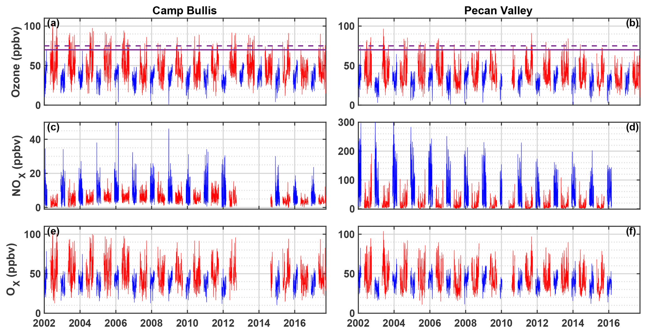
Figure 1 Time series of maximum daily average 8 h (MDA8) O₃, NO_x, and O_x at the Camp Bullis (a, c, e) and Pecan Valley (b, d, f) TCEQ sites for 2002–2017. Summer months (May–September) are shown in red, and winter months (December–February) are shown in blue. MDA8 is calculated by determining the maximum value of a species from running 8 h averages throughout the day. The purple dashed and solid red lines represent the 2008 (75 ppbv) and 2015 (70 ppbv) O₃ standards, respectively. Data were downloaded from https://www17.tceq.texas.gov/tamis/index.cfm?fuseaction=home.welcome (last access: 27 January 2019).

In this paper, we present results from the San Antonio Field Study (SAFS) conducted in the San Antonio, Texas, region in May 2017. We show observations of total peroxy radical concentrations ([XO₂] ≡ [RO₂] + [HO₂]) from three sites in the San Antonio area, characterizing the XO₂ distribution in the region. We use these XO₂ measurements, along with observations of NO and other trace gas species, to quantify ozone production in regions up- and downwind of the urban core. Though there have been many prior determinations of P(O₃) using measurements of a subset of peroxy radicals (i.e., using laser-induced fluorescence measurements of HO₂ and a fraction of RO₂) (e.g., Ren et al., 2013), this is one of the few determinations of ozone production using the direct observation of total peroxy radicals (Sommariva et al., 2011). Combined with quantification of the primary production of RO_x radicals (P(RO_x)) and satellite retrievals of HCHO and NO₂, we determine the ozone production regime in San Antonio. Finally, we explore the main contributors to OH reactivity in the region.

2 Methodology

2.1 Campaign description

The SAFS campaign was conducted from 11 to 31 May 2017 at several sites in the greater San Antonio region. We describe measurements made on the Aerodyne Mobile Laboratory (AML) at three sites: the University of Texas San Antonio (UTSA) from 11 to 16 May and from 27 to 31 May, Floresville, Texas, from 16 to 21 May, and Lake Corpus Christi (Corpus) from 21 to 26 May. The sites were chosen to determine the impact of various emission sources on ozone formation affecting San Antonio. During May in southeastern Texas, the prevailing wind direction is southeasterly, coming off the Gulf of Mexico. UTSA is located northwest (i.e. downwind) of downtown San Antonio (Fig. 2a), while the Floresville and Corpus sites were both located upwind of the city. This allows for the determination of background values of compounds through observation at the Floresville and Corpus sites, while observations at UTSA are more representative of air photochemically processed with urban emissions. We define background here as values upwind of the UTSA site. The AML was situated at all sites to minimize influence from local emissions. At UTSA, the AML was located in a mostly vacant parking lot about 1 km south of the nearest major roadway. In Floresville and Corpus, there were no nearby major roadways, local traffic was at a minimum, and influence from local point and mobile sources was limited. Potential influences from transient local sources (e.g., lawn mowers and jet skis) were removed in the same manner as interference from the generator emissions described below.

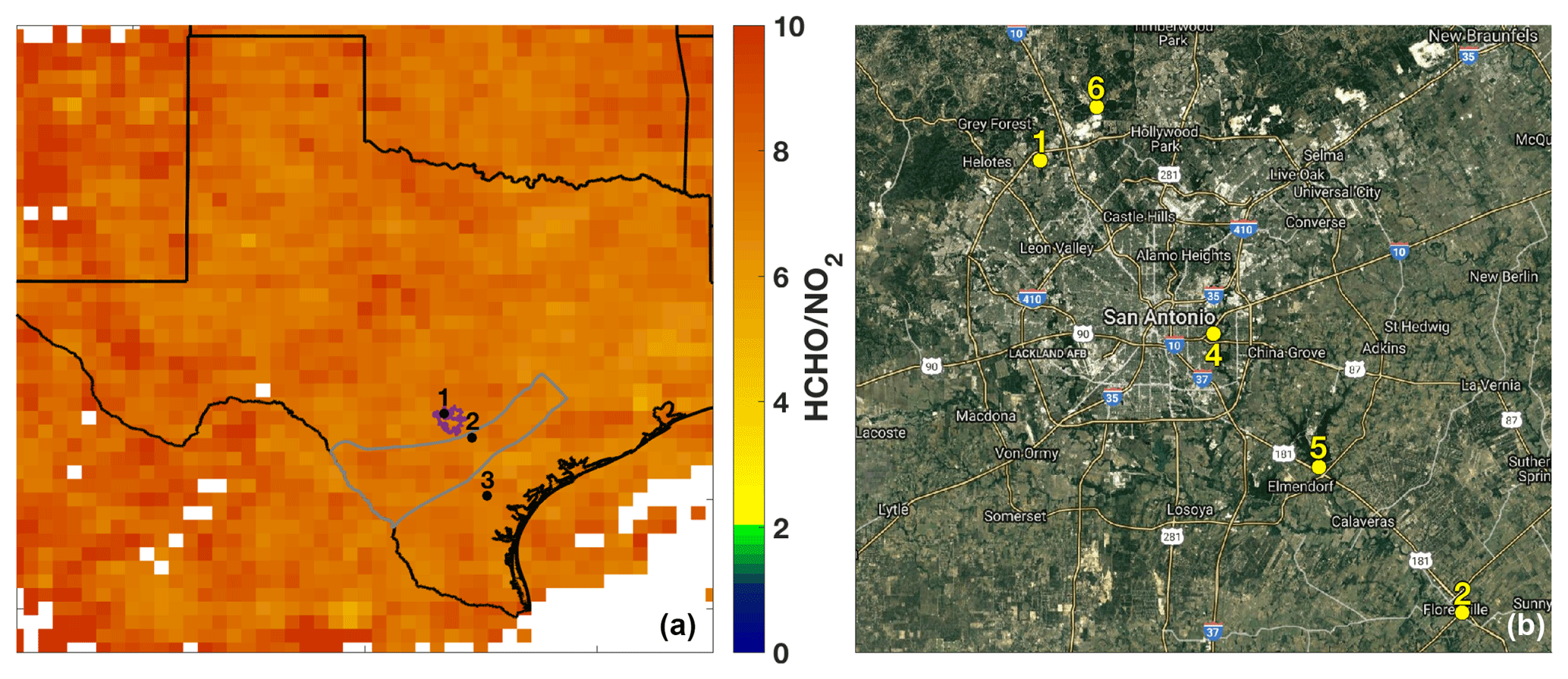
Figure 2 (a) The sampling locations for the AML are indicated: 1 – University of Texas San Antonio, 2 – Floresville, and 3 – Lake Corpus Christi. The ratio of total column HCHO to tropospheric column NO₂ averaged over the months of May through July 2017 is also shown for grid boxes with 10 or more observations of both species over the indicated time period. The outlines of the Eagle Ford Shale (grey) play and San Antonio city limits (purple) are also shown for reference. (b) The major roadways and TCEQ monitoring stations (6: Camp Bullis, 4: Pecan Valley, 5: Calaveras Lake) in the San Antonio region used in this study are shown. The UTSA and Floresville SAFS sites are also shown for reference.

The AML is outfitted to measure a suite of gas- and particle-phase atmospheric species (Herndon et al., 2005). All instrument inlets were mounted approximately 15 m above ground level on a retractable tower located near the AML. At both the Floresville and UTSA sites, the AML was powered through connection to the local electric utility, while at Corpus a diesel generator was used. Although the generator was situated downwind of the instrument inlets, some stagnation and recirculation did occur, allowing for occasional sampling of generator exhaust. Air parcels affected by the generator exhaust were removed through analysis of CO observations. A filter for generator-influenced air was created by determining the minimum CO value over a 100 s period every 5 min. Any air parcel with a CO mixing ratio 10 ppbv higher than this minimum was assumed to be impacted by a local transient source, including the generator.

Trace gases measured during SAFS and used in this study are summarized here. Unless otherwise indicated, data used in this study were reported as 1 min averages and then averaged to the 2 min Ethane CHemical AMPlifier (ECHAMP) time base, described in the following section. NO₂ was measured at 1 Hz via Cavity Attenuated Phase Shift (CAPS) spectroscopy (Kebabian et al., 2005, 2008). Nitric oxide (NO) was measured at 0.1 Hz through the same inlet as NO₂ and O₃ using a Thermo Fisher 42i-TL chemiluminescence analyzer, while O₃ was measured with a 2B-Tech model 205 ultraviolet (UV) absorption instrument. Uncertainties (2σ) of the NO, NO₂, and O₃ observations on the ECHAMP measurement timescale are below 5 %. The above instruments were zeroed every 15 min with humidity-matched zero air. The zero air was generated by passing ambient air through an Aadco ZA30 Catalyst system for VOC removal and through Purafil Chemisorbant Media, a potassium-permanganate-based scrubber, for NO_x removal.

Quantum Cascade Tunable Infrared Laser Direct Absorption Spectrometer (QC-TILDAS) instruments from Aerodyne Research Inc. (ARI) were used to measure CO and H₂O (2200 cm⁻¹; measurement wave number), HCHO (1765 cm⁻¹), CH₄ and C₂H₆ (2990 cm⁻¹), H₂O₂ (1277 cm⁻¹), and C₃H₈ (2965 cm⁻¹) (McManus et al., 2015). A proton-transfer-reaction high-resolution time-of-flight (PTR-HR-ToF) mass spectrometer was used to measure isoprene, acetaldehyde, acetone, benzene, methanol, the sum of monoterpenes, the sum of methyl vinyl ketone (MVK) and methacrolein, and toluene. Typical measurement uncertainties were on the order of 25 %. Finally, a prototype of a commercially available gas chromatograph from ARI with an electron-impact time-of-flight mass spectrometer (GC-EI-ToF-MS) was used to measure a suite of VOCs, including isoprene, 1,2,3-trimethylbenzene, ethylbenzene, cyclohexane, n-heptane, n-hexane, n-octane, n-pentane, o-xylene, and the sum of m- and p-xylenes. The GC sampled with a multicomponent adsorbent trap (Pollmann et al., 2006) for a 5 min integration period every 20 min. GC observations are unavailable for 20–30 May. While toluene and m- and p-xylene measurement uncertainty was on the order of 20 %, typical measurement uncertainties of other observed species, except isoprene, were on the order of 10 %.

While there were two independent observations of isoprene, there were limitations with both methods. It was determined that the actual isoprene concentration in the calibration standard used in the field for the PTR had degraded over time, resulting in erroneously high isoprene values. On the other hand, the GC was not calibrated for isoprene during the campaign, and observations are only available for half the time. As a result, we use the PTR isoprene from the entire campaign scaled to the GC values, using a GC isoprene sensitivity determined after the campaign. This method results in an estimated isoprene uncertainty of ≈30 % (1σ). See the Supplement for more information.

Temperature, wind speed, and wind direction were measured at the top of the inlet tower with a 3-D R.M. Young (Model 81000RE) sonic anemometer. Atmospheric pressure observations used in this study were taken from the National Weather Service observations at the San Antonio International Airport for the UTSA and Floresville sites and from the Corpus Christi International Airport for the Corpus site. NO₂ photolysis frequencies ($J_{{\mathrm{NO}}_{\mathrm{2}}}$) were measured via a filter radiometer (MetCon, GmbH) located on top of the AML (Shetter et al., 2003; Stark et al., 2007).

2.2 ECHAMP

Total peroxy radical concentrations ([XO₂]) were measured via chemical amplification by the ECHAMP instrument. A complete instrument description can be found in Wood et al. (2017), and only the most relevant details are summarized here, including a new sampling system that includes an integrated, remotely controlled RO_x calibration source. Briefly, ECHAMP measures total XO₂ concentration at a 2 min resolution by reacting peroxy radicals with excess NO and ethane (C₂H₆). Through a series of chain reactions, each XO₂ radical produces approximately 20 NO₂ molecules (depending on the relative humidity (RH)), which are then measured with a commercially available NO₂ monitor. Because this NO₂ monitor also measures ambient O₃ and NO₂ (O_x), a second channel and dedicated NO₂ monitor are used to only measure the sum of [O₃] and [NO₂]. The difference between the two channels, divided by the “amplification factor” of ≈20, yields the XO₂ concentration.

The inlet box is a 39 cm × 44 cm × 16 cm fiberglass, rainproof electrical enclosure. The box was mounted at the top of the sampling tower and connected to the rest of the instrument via a bundle of tubes and electrical cables. Ambient air was sampled at a flow rate of 6.5 L min⁻¹ through 76 mm of 3.6 mm inner diameter glass into the inlet box (see Supplement Fig. S1 for a schematic of the plumbing). The glass was internally coated with halocarbon wax to minimize wall losses of XO₂. The flow was subsampled into two 1.9 cm³ reaction chambers at a flow rate of 1.1 L min⁻¹ each. Temperature and RH of the remaining 4.5 L min⁻¹ of sampled air were measured with a Vaisala probe (Model HMP60). Laboratory tests over a range of flow rates and RH have demonstrated sampling losses of HO₂ of less than 3 % and negligible losses of CH₃O₂ (Kundu et al., 2019).

Reaction chambers cycled every minute between an amplification mode and a background mode, for a total cycle time of 2 min. In both modes, 25 sccm of 39.3 ppmv NO in N₂ (Praxair) was added at the beginning of the reaction chamber, resulting in a final NO mixing ratio of 0.90 ppmv. In amplification mode, 35 sccm of a 42.2 % ethane mixture in N₂ (Praxair) was also added to the sampled air at the beginning of the reaction chamber. The radical propagation scheme shown in Reactions (R7)–(R13), in which Reactions (R9)–(R13) repeat numerous times, results in the formation of NO₂. The number of NO₂ molecules formed per XO₂ molecule sampled is known as the amplification factor (F) and varies with RH. During SAFS, F was 23 for dry air and decreased to 12 at 58 % RH. The two calibration methods used to determine F are described below and more fully in the Supplement. At 15.2 cm downstream of the NO∕C₂H₆ injection point, 35 sccm of N₂ was added to the flow. In the background chamber, the N₂ and C₂H₆ flows were switched (N₂ was added upstream, and C₂H₆ was added downstream), allowing XO₂ radicals to react with NO to form HONO or alkyl nitrates before 35 sccm of the 42.2 % ethane mixture was added at the end of the reaction chamber. The resultant NO₂ from each chamber was then measured with separate, dedicated CAPS instruments. Total XO₂ was then determined by the difference between the two NO₂ measurements divided by F.

$$\begin{array}{}\text{(R7)}& {\displaystyle }& {\displaystyle }{\mathrm{RO}}_{\mathrm{2}}+\mathrm{NO}\to \mathrm{RO}+{\mathrm{NO}}_{\mathrm{2}}\text{(R8)}& {\displaystyle }& {\displaystyle }\mathrm{RO}\to {\mathrm{HO}}_{\mathrm{2}}+\mathrm{products}\text{(R9)}& {\displaystyle }& {\displaystyle }{\mathrm{HO}}_{\mathrm{2}}+\mathrm{NO}\to \mathrm{OH}+{\mathrm{NO}}_{\mathrm{2}}\text{(R10)}& {\displaystyle }& {\displaystyle }\mathrm{OH}+{\mathrm{C}}_{\mathrm{2}}{\mathrm{H}}_{\mathrm{6}}\to {\mathrm{H}}_{\mathrm{2}}\mathrm{O}+{\mathrm{C}}_{\mathrm{2}}{\mathrm{H}}_{\mathrm{5}}\text{(R11)}& {\displaystyle }& {\displaystyle }{\mathrm{C}}_{\mathrm{2}}{\mathrm{H}}_{\mathrm{5}}+{\mathrm{O}}_{\mathrm{2}}+\mathrm{M}\to {\mathrm{C}}_{\mathrm{2}}{\mathrm{H}}_{\mathrm{5}}{\mathrm{O}}_{\mathrm{2}}+\mathrm{M}\text{(R12)}& {\displaystyle }& {\displaystyle }{\mathrm{C}}_{\mathrm{2}}{\mathrm{H}}_{\mathrm{5}}{\mathrm{O}}_{\mathrm{2}}+\mathrm{NO}\to {\mathrm{C}}_{\mathrm{2}}{\mathrm{H}}_{\mathrm{5}}\mathrm{O}+{\mathrm{NO}}_{\mathrm{2}}\text{(R13)}& {\displaystyle }& {\displaystyle }{\mathrm{C}}_{\mathrm{2}}{\mathrm{H}}_{\mathrm{5}}\mathrm{O}+{\mathrm{O}}_{\mathrm{2}}\to {\mathrm{CH}}_{\mathrm{3}}\mathrm{CHO}+{\mathrm{HO}}_{\mathrm{2}}\end{array}$$

The CAPS instruments were calibrated for NO₂ before, after, and once during deployment via the quantitative reaction of known concentrations of O₃ generated with a 2B Technologies ozone generator (Model 306) with excess NO. This ozone source agreed within 1 % with a separate Thermo ozone generation source (Model 49C). All NO₂ calibrations agreed within 5 %. The amplification factor (F) was determined by producing known amounts of peroxy radicals with two calibration methods: photolysis of H₂O and of CH₃I. Both methods are described in more detail in the Supplement. Briefly, the H₂O photolysis method is similar to that used by most HO_x instruments, in which H₂O was photolyzed at a wavelength of 184.9 nm to form an equimolar mixture of OH and HO₂ (Mihele and Hastie, 2000; Faloona et al., 2004). This mixture was then reacted with H₂ to convert the OH into HO₂. Radical concentrations were quantified using the relevant spectroscopic parameters and the measured H₂O and O₃ concentrations in the calibration gas.

The second calibration method was based on 254 nm photolysis of CH₃I in humidified air, producing the CH₃O₂ radical. The radical concentration is quantified by reaction of the CH₃O₂ with NO in the absence of C₂H₆, producing 1.86 NO₂ molecules per CH₃O₂. The H₂O photolysis method was performed six times, while the CH₃I method was performed once during the field campaign, on 31 May. Both methods were repeated twice in the laboratory after the campaign. Observations from ECHAMP agreed within 12 % with the H₂O photolysis calibration source operated by Indiana University during a comparison study in 2015 (Kundu et al., 2019). For the XO₂ observations described in this paper, we use the CH₃I calibration. While both methods agree within uncertainty, the H₂O photolysis method was only conducted for RH values of less than approximately 20 %, much lower than typical ambient RH. See the Supplement for further information.

The total 2σ accuracy for XO₂ during SAFS was approximately 25 %. Calibrations were not performed at RH values greater than 71 %. Therefore, we omit all observations with a sample RH greater than 71 %. Approximately 85 % of these high RH points were observed at nighttime, so we only consider daytime data (07:00–20:00 local time) unless otherwise indicated.

2.3 Calculation of P(O₃) and P(RO_x)

We use measurements of XO₂ and NO to calculate the gross rate of ozone production P(O₃) using Eq. (2), in which $k_{\mathrm{NO}+{\mathrm{HO}}_{\mathrm{2}}}$ is the reaction constant for the reaction of NO with HO₂ and k_i is the reaction constant for NO with an organic peroxy radical [RO₂]_i. We note that this is more accurately described as the rate of odd oxygen (O_x) production. Because ECHAMP only measures the sum of peroxy radicals and not their speciation, we assume a simplified form of this relationship (Eq. 3), where k_eff is an effective rate constant taken as that of $k_{\mathrm{NO}+{\mathrm{HO}}_{\mathrm{2}}}$. Box modeling results for this site, which will be discussed more fully in a forthcoming paper, show the dominant XO₂ species are HO₂, CH₃O₂, and isoprene RO₂. At 298 K, $k_{\mathrm{NO}+{\mathrm{HO}}_{\mathrm{2}}}$ is within 10 % of the k values for the reaction of NO with CH₃O₂ and isoprene RO₂ (Orlando and Tyndall, 2012), supporting our choice of k_eff. Further, while the reaction of NO with acetyl peroxy radicals is approximately 2.5 times faster than with other peroxy radicals at 298 K, box modeling results suggest that these radicals comprise only 5 %–10 % of total XO₂, resulting in an average difference in P(O₃) of 15 % from the $k_{\mathrm{NO}+{\mathrm{HO}}_{\mathrm{2}}}$ value used here. This uncertainty is comparable to the total uncertainty of the $k_{\mathrm{NO}+{\mathrm{HO}}_{\mathrm{2}}}$ rate constant, estimated as 15 % (Sanders et al., 2011). As will be shown in Sect. 3.2, our conclusions are insensitive to the value of k_eff chosen. Uncertainty in gross P(O₃) results from uncertainty in the NO and XO₂ measurements, 5 % and 25 %, respectively, and k_eff, whose uncertainty we estimate at 23 %, determined by adding the uncertainty in the $k_{\mathrm{NO}+{\mathrm{HO}}_{\mathrm{2}}}$ rate constant and the uncertainty in the choice of k_eff in quadrature. This results in a total P(O₃) uncertainty of 34 %.

$$\begin{array}{ll}\text{(2)}& {\displaystyle }& {\displaystyle }{P\left({\mathrm{O}}_{\mathrm{3}}\right)}_{\mathrm{Gross}}=k_{\mathrm{NO}+{\mathrm{HO}}_{\mathrm{2}}}\left[\mathrm{NO}\right]\left[{\mathrm{HO}}_{\mathrm{2}}\right]+\left[\mathrm{NO}\right]\sum _i{k}_i[{\mathrm{RO}}_{\mathrm{2}}{]}_i\text{(3)}& {\displaystyle }& {\displaystyle }{P\left({\mathrm{O}}_{\mathrm{3}}\right)}_{\mathrm{Gross}}=k_{\mathrm{eff}}\left[\mathrm{NO}\right]\left[X{\mathrm{O}}_{\mathrm{2}}\right]{\displaystyle }& {\displaystyle }L\left({\mathrm{O}}_{\mathrm{3}}\right)=\\ {\displaystyle }& {\displaystyle }\left({\displaystyle \frac{k_{{\mathrm{O}}^{\mathrm{1}}\mathrm{D}+{\mathrm{H}}_{\mathrm{2}}\mathrm{O}}\left[{\mathrm{H}}_{\mathrm{2}}\mathrm{O}\right]}{k_{{\mathrm{O}}^{\mathrm{1}}\mathrm{D}+{\mathrm{H}}_{\mathrm{2}}\mathrm{O}}\left[{\mathrm{H}}_{\mathrm{2}}\mathrm{O}\right]+k_{{\mathrm{O}}^{\mathrm{1}}\mathrm{D}+{\mathrm{N}}_{\mathrm{2}}}\left[{\mathrm{N}}_{\mathrm{2}}\right]+k_{{\mathrm{O}}^{\mathrm{1}}\mathrm{D}+\mathrm{O}\mathrm{2}}\left[{\mathrm{O}}_{\mathrm{2}}\right]}}{J}_{{\mathrm{O}}^{\mathrm{1}}\mathrm{D}}\right.\\ {\displaystyle }& {\displaystyle }+k_{\mathrm{OH}+{\mathrm{O}}_{\mathrm{3}}}\left[\mathrm{OH}\right]+k_{{\mathrm{HO}}_{\mathrm{2}}+{\mathrm{O}}_{\mathrm{3}}}\left[{\mathrm{HO}}_{\mathrm{2}}\right]+\sum _i\\ \text{(4)}& {\displaystyle }& {\displaystyle }\left.k_{\mathrm{alkene}-i}\left[{\mathrm{alkene}}_i\right]\right)\left[{\mathrm{O}}_{\mathrm{3}}\right]+k_{\mathrm{OH}+{\mathrm{NO}}_{\mathrm{2}}}\left[\mathrm{OH}\right]\left[{\mathrm{NO}}_{\mathrm{2}}\right]\left[\mathrm{M}\right]\end{array}$$

The net formation rate of O₃ is equal to P(O₃)_Gross – L(O₃). In order to tie P(O₃) completely to observations, we report only gross P(O₃), not net P(O₃). That is, we only calculate the production term (Eq. 2) and not the loss term (Eq. 4) for net ozone production. Calculation of the loss term requires knowledge of the concentration of OH and alkenes as well as the fraction of total XO₂ comprised of HO₂. Of these quantities, only a small subset of alkenes – isoprene and monoterpenes – were measured during SAFS. Estimating the alkene loss term using concentrations from nearby TCEQ monitoring sites suggests that O₃ loss due to this pathway is negligible for the data analyzed here, and we omit this from our calculation of ozone loss. To estimate OH and the fraction of XO₂ comprised of HO₂ and to determine whether analyzing only gross P(O₃) affects our conclusions, we used the Framework for 0-Dimensional Atmospheric Modeling (F0AM) box model (Wolfe et al., 2016b) to calculate OH and the fraction of RO₂ comprised of HO₂. A description of the model setup can be found in the Supplement. For data points that were not modeled due to missing model constraints, these values were estimated from the interpolation of modeled values, if observations were made within 2 h of a modeled data point, or from site-specific mean daily profiles if no modeled points were available. Using these modeled-derived values for OH and the HO₂ fraction, median L(O₃) for daytime observations at all sites was determined to be 0.90 ppbv h⁻¹, which is 16 % of the gross production rate.

We use Eq. (5) to calculate the primary RO_x production rate. Here, P(RO_x) is the RO_x production rate, J indicates photolysis rate, and $k_{{\mathrm{O}}^{\mathrm{1}}\mathrm{D}+{\mathrm{H}}_{\mathrm{2}}\mathrm{O}}$, $k_{{\mathrm{O}}^{\mathrm{1}}\mathrm{D}+{\mathrm{O}}_{\mathrm{2}}}$, and $k_{{\mathrm{O}}^{\mathrm{1}}\mathrm{D}+{\mathrm{N}}_{\mathrm{2}}}$ are the reaction rate constants for the reaction of ${\mathrm{O}}_{{}^{\mathrm{1}}\mathrm{D}}$ with the indicated species. The Tropospheric Ultraviolet and Visible (TUV) model was used to calculate photolysis rate constants (J values), which were then scaled to the measured $J_{{\mathrm{NO}}_{\mathrm{2}}}$. HONO was not measured during SAFS. We estimate HONO concentrations assuming an upper limit to the [HONO]∕[NO_x] ratio of 0.04 as described in Lee et al. (2013). This is an upper bound on the HONO concentration and thus on HONO contribution to P(RO_x). Alkene concentrations were estimated from nearby TCEQ monitoring sites, as described in Sect. 3.3. Alkene ozonolysis was calculated to have a negligible impact on P(RO_x) and is omitted from the analysis.

$$\begin{array}{ll}{\displaystyle }& {\displaystyle }P\left({\mathrm{RO}}_x\right)=\\ {\displaystyle }& {\displaystyle }\mathrm{2}{J}_{{\mathrm{O}}^{\mathrm{1}}\mathrm{D}}\left[{\mathrm{O}}_{\mathrm{3}}\right]{\displaystyle \frac{k_{{\mathrm{O}}^{\mathrm{1}}\mathrm{D}+{\mathrm{H}}_{\mathrm{2}}\mathrm{O}}\left[{\mathrm{H}}_{\mathrm{2}}\mathrm{O}\right]}{k_{{\mathrm{O}}^{\mathrm{1}}\mathrm{D}+{\mathrm{H}}_{\mathrm{2}}\mathrm{O}}\left[{\mathrm{H}}_{\mathrm{2}}\mathrm{O}\right]+k_{{\mathrm{O}}^{\mathrm{1}}\mathrm{D}+{\mathrm{N}}_{\mathrm{2}}}\left[{\mathrm{N}}_{\mathrm{2}}\right]+k_{{\mathrm{O}}^{\mathrm{1}}\mathrm{D}+{\mathrm{O}}_{\mathrm{2}}}\left[{\mathrm{O}}_{\mathrm{2}}\right]}}\\ {\displaystyle }& {\displaystyle }+\mathrm{2}{J}_{\mathrm{HCHO}}\left[\mathrm{HCHO}\right]+\mathrm{2}{J}_{{\mathrm{CH}}_{\mathrm{3}}\mathrm{CHO}}\left[{\mathrm{CH}}_{\mathrm{3}}\mathrm{CHO}\right]\\ {\displaystyle }& {\displaystyle }+\mathrm{2}{J}_{\mathrm{Acetone}}\left[{\mathrm{CH}}_{\mathrm{3}}{\mathrm{COCH}}_{\mathrm{3}}\right]+\mathrm{2}{J}_{{\mathrm{H}}_{\mathrm{2}}{\mathrm{O}}_{\mathrm{2}}}\left[{\mathrm{H}}_{\mathrm{2}}{\mathrm{O}}_{\mathrm{2}}\right]\\ \text{(5)}& {\displaystyle }& {\displaystyle }+J_{\mathrm{HONO}}\left[\mathrm{HONO}\right]\end{array}$$

Total P(RO_x) peaks at midday at about 0.65 pptv s⁻¹ on average and is dominated by the ozone and HCHO terms, terms 1 and 2 from Eq. (5), respectively, with contributions from the other observed species totaling less than 5 % on average. Contributions from HONO were generally less than 0.1 pptv s⁻¹, even assuming the upper bound in the HONO to NO_x ratio used here.

2.4 Satellite data

We use observations of NO₂ and HCHO from the Ozone Monitoring Instrument (OMI) to provide a remotely sensed estimate of the surface ozone production regime in San Antonio (Duncan et al., 2010; Ring et al., 2018). OMI has a local overpass time of about 13:30 and provides daily, global coverage. The instrument measures backscattered solar radiation in the UV–visible region, allowing for differential optical absorption spectroscopy (DOAS)-type retrievals of multiple species, including NO₂ and HCHO.

For NO₂, we use the NASA Goddard Space Flight Center (GSFC) version 3 level 2 tropospheric column product (Bucsela et al., 2013; Krotkov et al., 2017) gridded to 0.25^∘ latitude ×0.25^∘ longitude resolution. For HCHO, we use the version 3 level 2 reference-sector-corrected swath product from the Harvard Smithsonian Astrophysical Observatory (SAO) retrieval (González Abad et al., 2015) also on a 0.25^∘ latitude ×0.25^∘ longitude grid. For both OMI products, we only use pixels that satisfy quality and row anomaly flags, have a cloud fraction less than 30 %, and have a solar zenith angle less than 70 ^∘. Additionally, data from the two outer most pixels are removed due to their large footprint (28 km × 150 km) compared to the nadir view.

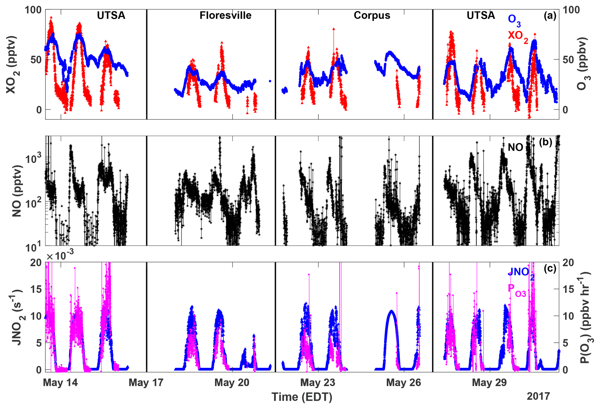
Figure 3 Time series of O₃ (blue circles), XO₂ (red triangles), NO (black stars), JNO₂ (blue triangles), and P(O₃) (magenta circles) measured at all sites. All data are averaged over the XO₂ sampling period.

We analyze the HCHO to NO₂ ratio using OMI data from May to July 2017. While SAFS only lasted 1 month, missing data due to cloud cover, the row anomaly, and other factors necessitate a longer time period for data averaging. To calculate the ratio of HCHO to NO₂, we first calculate the standard deviations (σ) of the HCHO and NO₂ data at each grid point. When calculating the ratio, we only include days within 2σ of the average HCHO and NO₂ observations and only include grid boxes that have at least 10 days with coincident observations of both species.

3 Results

3.1 Distribution of ozone and its precursors

The highest ozone mixing ratios observed at UTSA were on 14 and 15 May, reaching a maximum near 80 ppbv, while daytime values typically varied between 40 and 60 ppbv during the remainder of the campaign (Fig. 3). Median daytime [O₃] at all three measurement sites was 37 ppbv (Fig. 4a). Median ozone was 18 ppbv higher at UTSA than at the background site in Floresville. Although the highest ozone values were seen at UTSA, there was significant overlap in the ozone distribution between the UTSA and Corpus sites. Consistent with the higher O₃ abundance, concentrations of the O₃ precursors isoprene, NO, and XO₂ were also highest at the UTSA site. Median isoprene concentrations, one of the largest contributors to OH reactivity, as will be shown later, were almost 2 orders of magnitude larger at UTSA (1.2 ppbv) than at the other sites (0.05 and 0.03 ppbv at Floresville and Corpus, respectively). While the difference in median [NO] at the sites was not as extreme, a much larger range was seen at UTSA, where the 95th percentile of observations was above 2 ppbv. Similar results are seen for the [XO₂] distribution (Fig. 4c), with the highest XO₂ mixing ratios (90 pptv) coinciding with the maximum O₃. Median [XO₂] was approximately 1.5 times higher at the UTSA site (37 pptv) than at Floresville (26 pptv) and Corpus (25 pptv).

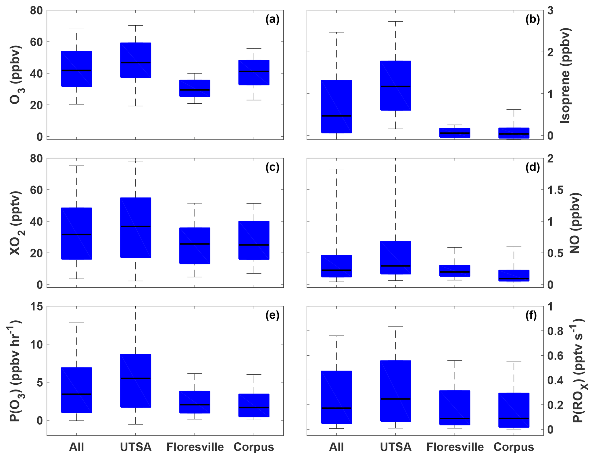
Figure 4 The distribution of O₃ (a), isoprene (b), XO₂ (c), NO (d), P(O₃) (e), and P(RO_x) (f) for all observations during SAFS taken between 07:00 and 20:00. The distribution for the entire campaign (All) as well as at the individual sites is shown. Medians are indicated by the black lines, and the 5th, 25th, 75th, and 95th percentiles are shown by the edges of the boxes and whiskers.

XO₂ concentrations showed a distinct diurnal profile (Fig. 5). Overnight values were approximately constant with a median of around 10 pptv, until a small decline after 03:00. A steady increase in [XO₂] began at 09:00, with a peak of 50 pptv at 15:00 and then a decline to the overnight value by 20:00. The shape of this profile is in agreement with other observations of peroxy radicals from a variety of chemical environments (Sanchez et al., 2016; Mao et al., 2010; Whalley et al., 2018). Noise in the nighttime data is a result of higher RH and thus degraded precision of the ECHAMP measurement technique and is not an indication of significant nighttime variability. Even though we have filtered for data points with RH greater than 71 % as discussed in Sect. 2.2, nighttime RH is higher than daytime values, on average, decreasing measurement precision. Daytime variability resulted from changes in insolation and biogenic VOC concentrations. The days that showed little or no diurnal profile at UTSA and Corpus were overcast, as evidenced by low $J_{{\mathrm{NO}}_{\mathrm{2}}}$ (Fig. 3). Concentrations of isoprene and the sum of methyl vinyl ketone (MVK) and methacrolein, both isoprene degradation products, were at a maximum when [XO₂] peaked at 90 pptv.

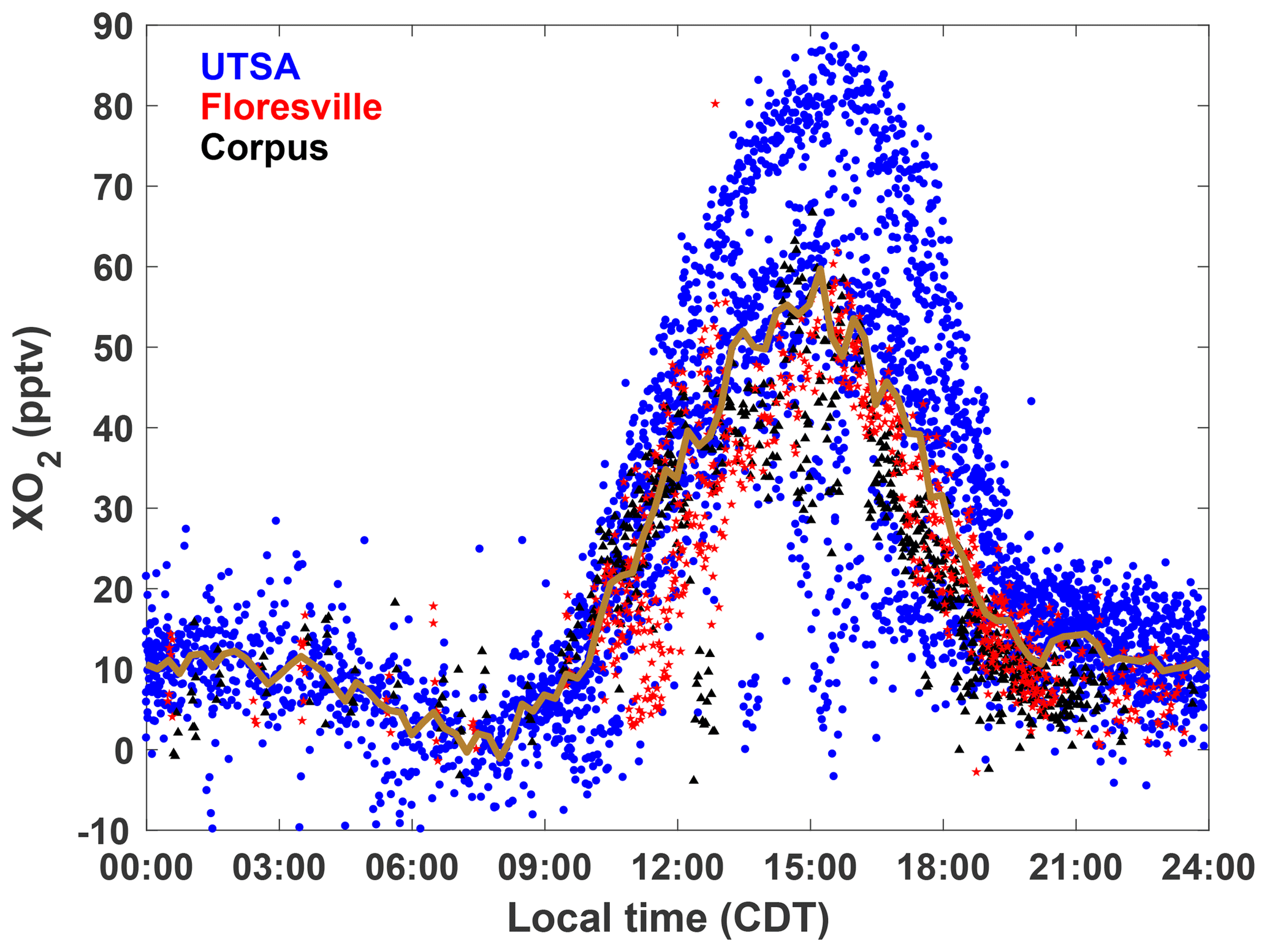
Figure 5 The diurnal profile of all 2 min average XO₂ observations made during SAFS. Observations made at UTSA are shown in blue, Floresville in red, and Corpus in black. The median value for 15 min time bins for observations at all sites is shown by the gold trace.

The higher O₃ concentrations at UTSA are consistent with its location downwind of the urban core of San Antonio. Figure S2 shows wind roses colored by ozone and the ozone precursors described above. The wind direction while at UTSA was predominantly southeasterly, in agreement with the climatological average for the region. The highest ozone mixing ratios, as well as the highest XO₂ and isoprene, were seen when air parcels originated from this direction, traveling over the city. The highest [NO] (greater than 2.2 ppbv), however, was seen with northerly and northeasterly winds. This is likely because of the proximity of a major highway north of the UTSA site, which would provide a source of recently emitted, less processed emissions than in air parcels that traveled from downtown San Antonio. The CO distribution by wind direction (not shown) is consistent with this explanation.

3.2 Ozone production

The highest P(O₃) values (and highest [NO] and [XO₂]) were observed at UTSA. Median P(O₃) between 07:00 and 20:00 at UTSA was 4.1  ppbv h⁻¹, compared to just over 1 ppbv h⁻¹ at both Floresville and Corpus. The 95th percentile, 12.6 ppbv h⁻¹, is significantly lower than rates found in Houston, which frequently topped 40 ppbv h⁻¹ (Mazzuca et al., 2016; Mao et al., 2010). As with [O₃] and [XO₂], the highest P(O₃) rates occurred when winds traveled over downtown San Antonio.

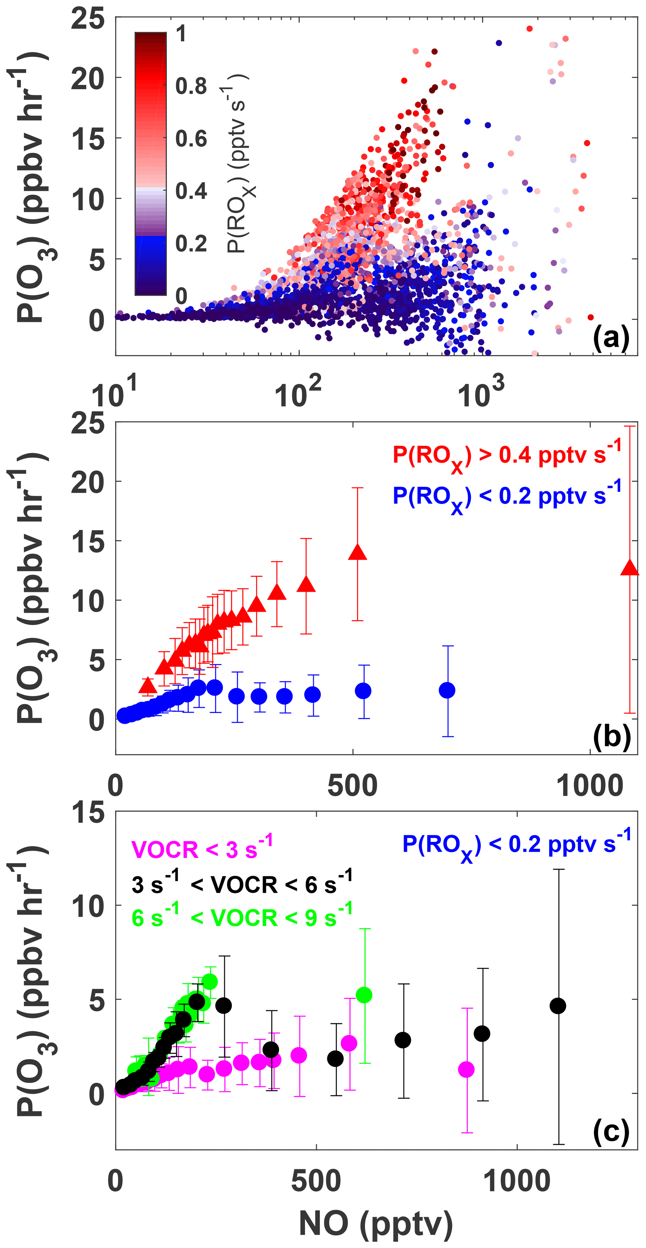
Figure 6 The variation of P(O₃) with NO for all daytime observations (07:00 to 20:00) made during SAFS (a). Observations are colored by P(RO_x). The same data as shown in panel (a) but sorted by P(RO_x) are shown in panel (b). Observations with P(RO_x) greater than 0.4 pptv s⁻¹ are shown in red, while observations with P(RO_x) less than 0.2 pptv s⁻¹ are shown in blue. Data are separated into NO bins with an equal number of observations per bin. The mean value of each bin is shown, with the error bars showing 1 standard deviation. The subset of observations with P(RO_x) <0.2 pptv s⁻¹ is further separated into three categories: low VOC reactivity (VOCR <3 s⁻¹; magenta), medium VOC reactivity (3 < VOCR < 6 s⁻¹; black), and high VOC reactivity (6 < VOCR < 9 s⁻¹; green) (c). As in panel (b) data are separated into NO bins with equal numbers of observations in each bin.

Figure 6a shows the variation in P(O₃) with [NO], for which the data points have been colored by P(RO_x) for all observations taken during SAFS. The relationship for the subset of observations exclusively at UTSA is essentially identical. In general, P(O₃) increases with [NO], although a wide range of P(O₃) exists for a given value of NO. For a constant value of [NO], P(O₃) is consistently higher at higher P(RO_x). Figure 6b shows the same data as panel 6a but binned both by NO mixing ratio and P(RO_x). All P(O₃) observations have been separated into NO bins with an equal number of observations, as well as into two bins of P(RO_x) < 0.2 and P(RO_x) > 0.4. The values of P(RO_x) were chosen to represent the low and high ranges of P(RO_x) observed during SAFS. The conclusions drawn from the results are insensitive to the values chosen for these bins.

Figure 6b demonstrates that the majority of observations made during SAFS were in the NO_x-limited regime. For the high P(RO_x) observations, there is a steady increase in P(O₃) up to the 500 pptv NO bin. Above this point, P(O₃) potentially plateaus, but there were insufficient observations at higher NO to determine the location of the turnover point in ozone production. Because the majority of NO observations at UTSA were less than 500 pptv, we conclude that the site is predominantly NO_x-limited. Further observations at higher NO mixing ratios are required to determine the turnover point for ozone production in this region. The true turnover concentration for NO cannot be easily inferred by inspection of a graph of P(O₃) versus [NO], however, because VOC concentrations are not constant for all points. To see if there is any variation in this relationship with VOCs, we further separate the high P(RO_x) data by their VOC reactivity (Fig. S3). VOC reactivity (VOCR) was calculated in the same manner as OH reactivity, described in Sect. 3.3, but including only OH reactive VOCs. In addition, VOCs exclusively observed by the GC instrument were not included in the calculation as they were only available until 19 May. For data points with GC observations available, VOC reactivity increased by only 2 % in the afternoon and 12 % in the morning on average when including the GC observations, suggesting that this omission does not significantly affect the results. Data were then separated into low (VOCR < 3 s⁻¹), medium (3 s⁻¹ < VOCR < 6 s⁻¹), and high (6 s⁻¹ < VOCR < 9 s⁻¹) VOC reactivity bins. For the high P(RO_x) case, the relationship is similar for all VOC reactivities, showing a general increase in P(O₃) with NO, further suggesting the majority of observations were NO_x-limited for high P(RO_x). We note that for a constant P(RO_x) value, theoretically P(O₃) is expected to increase with [NO] at approximately the same rate until the turnover point with little sensitivity to the VOC reactivity. The 5th and 95th percentiles of P(RO_x) for the high P(RO_x) are 0.42 and 0.92 pptv s⁻¹, more than a factor of 2 different. This suggests that the differences in the rate of change of P(O₃) with NO for the different VOC reactivities likely result from the wide range of P(RO_x) values analyzed.

When looking at all points for the low P(RO_x) case (Fig. 6b), there is a small peak in P(O₃) at 200 pptv NO, suggesting that in a low P(RO_x) environment, UTSA can be VOC-limited at higher NO mixing ratios. Separating these data points by VOC reactivity shows more clearly the transition between the NO_x- and VOC-limited regimes. For the medium case, P(O₃) first increases with [NO], peaks at 5 ppbv h⁻¹ at approximately 200 pptv [NO], and then declines to 2 ppbv h⁻¹ at 400 pptv [NO]. This peak and decline suggests that, for P(RO_x) < 0.2 pptv s⁻¹, VOC reactivities < 6 s⁻¹, and NO > 200 pptv, the region is VOC-limited. For NO > 400 pptv, there is a slight increase in P(O₃) with [NO], although the spread of data for a given [NO] also increases. For the low VOC reactivity scenario, the range of P(O₃) for a given [NO] is also large compared to the mean P(O₃), making it difficult to determine whether these points obey a similar relationship. As with the high P(RO_x) scenario, each bin has a wide range of P(RO_x) and VOC reactivities, which could lead to the large spread in data, suggesting the need for further observations. Separating the data by location yields the same results, although VOC reactivity at Floresville and Corpus was almost always below 3 s⁻¹ due to the lower isoprene concentration at these sites in comparison to UTSA.

Ozone production rates in a VOC-limited regime are typically below 5 ppbv h⁻¹ and constitute only 20 % of the observations examined here, suggesting that all three SAFS sites are predominantly NO_x-limited. The majority of the VOC-limited points here (75 %) occur before 11:00 EDT, when NO concentrations are higher and isoprene emissions and VOC reactivity are low. This is in agreement with the L_N∕Q diurnal profile discussed below. For the NO_x-limited points, increases in VOC concentrations are expected to have a small impact on P(O₃); for the VOC-limited points, increases in VOCs will lead to increased P(O₃).

Finally, the results presented here are insensitive to the value of k_eff chosen. Figure S4 shows the relationship between P(O₃) and NO for four different values of k_eff: $k_{\mathrm{NO}+{\mathrm{HO}}_{\mathrm{2}}}$ (the k_eff used in this analysis), $k_{\mathrm{NO}+{\mathrm{CH}}_{\mathrm{3}}{\mathrm{O}}_{\mathrm{2}}}$, $k_{\mathrm{NO}+{\mathrm{IsopreneRO}}_{\mathrm{2}}}$, and assuming k_{NO+acetyl peroxy} for 10 % of the value and $k_{\mathrm{NO}+{\mathrm{HO}}_{\mathrm{2}}}$ for the remainder. While the magnitude of P(O₃) does change with k_eff, the overall relationship is the same. As mentioned previously, the uncertainty in $k_{\mathrm{NO}+{\mathrm{HO}}_{\mathrm{2}}}$ is larger than the uncertainty induced by the choice of k_eff. Additional analysis further suggests that the majority of the observations during SAFS were in the NO_x-limited regime.

These results are consistent with the diurnal profile of the ozone production regime as determined by the separate “L_N∕Q” metric, which is the ratio of the RO_x loss rate due to reactions with NO_x to the total RO_x loss rate (Q) (Kleinman, 2005). In general, when more than half of the RO_x loss is due to reaction with NO_x species (L_N∕Q > 0.5) then P(O₃) is VOC-limited, whereas when the majority of RO_x loss is due to peroxy radical self-reactions (L_N∕Q < 0.5) P(O₃) is NO_x-limited. The Framework for 0-Dimensional Atmospheric Modeling (F0AM) photochemical box model (Wolfe et al., 2016b), constrained to observations, was used to model the parameters needed to calculate L_N∕Q at the SAFS sites. A full description of the model setup is in the Supplement. Using the box model results and the method described in Kleinman (2005), we calculated L_N∕Q for all box-modeled observations at UTSA (Fig. 7). A clear diurnal pattern is evident with an early morning maximum and then a quick decline to L_N∕Q < 0.5 at 09:00, after which the ratio remains below 0.1 for the remainder of the day. At 18:00, however, the ratio does begin to increase, though it remains well in the NO_x-limited space. While L_N∕Q is highest in the morning, P(O₃) is at a minimum during this time period, suggesting that there is little O₃ production when P(O₃) is VOC-limited. Furthermore, time periods during which ozone was found under VOC-limited conditions were likely confined to a relatively small volume of air in the shallow, morning boundary layer. This transition from a VOC- to NO_x-limited regime between morning and afternoon is consistent with other locations (Mazzuca et al., 2016; Mao et al., 2010; Ren et al., 2013) and the high NO concentrations that build up in the morning from local traffic and a low boundary layer.

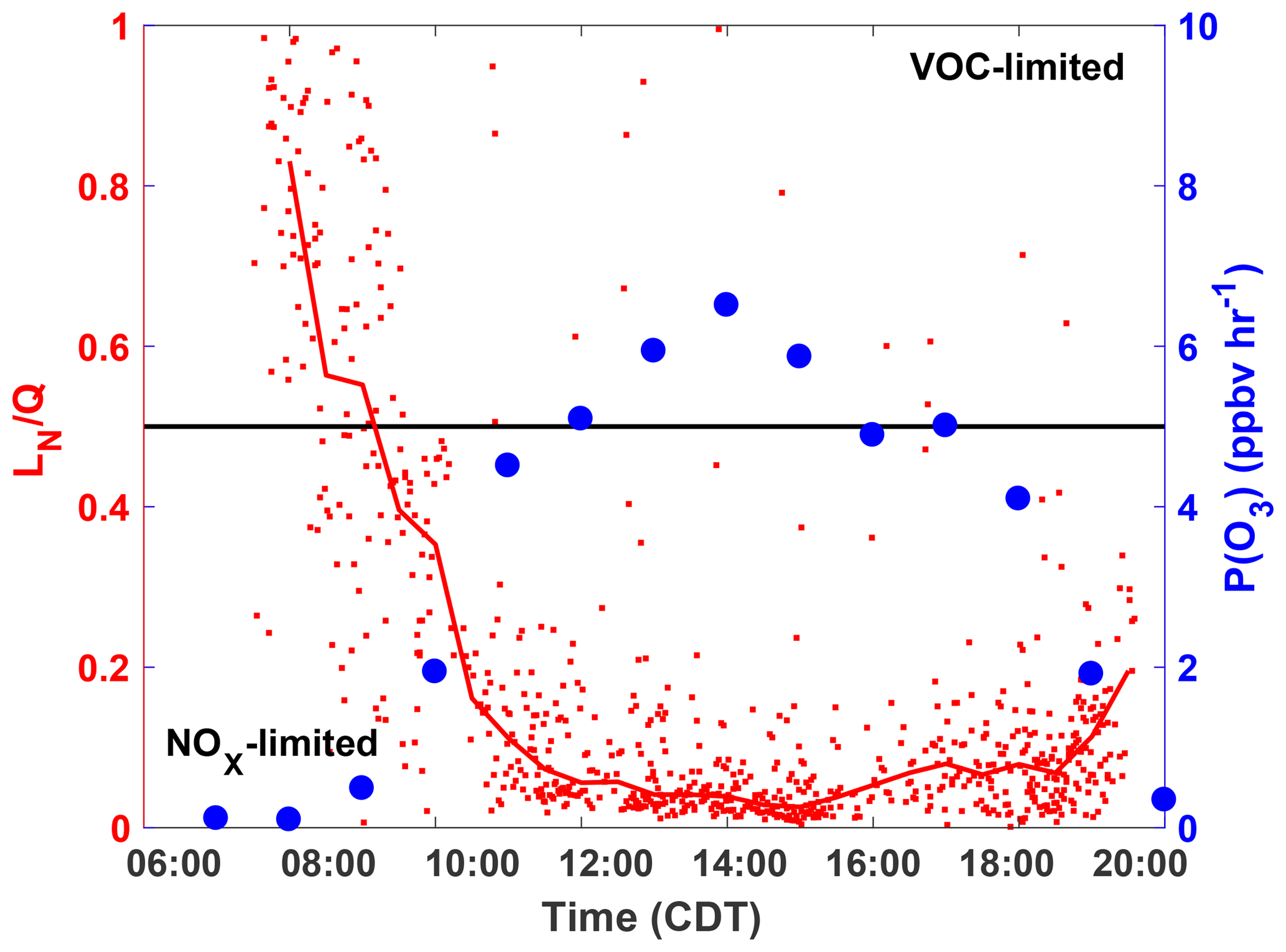
Figure 7 The diurnal profiles of L_N∕Q calculated with the F0AM box model (red), and the median P(O₃) in 1 h time bins (blue). The median L_N∕Q value for half hour bins is shown by the red line. Profiles are only for observations at UTSA. Points are calculated by P(O₃) calculated from observations. The black line is approximately the separation between the NO_x- and VOC-limited regimes.

Finally, remotely sensed observations of NO₂ and HCHO from the OMI satellite corroborate the conclusion that ozone production in San Antonio is NO_x-limited. The ratio of column HCHO to tropospheric column NO₂ has been used as an indicator of the ozone production regime in multiple regions (Duncan et al., 2010; Ring et al., 2018). According to Duncan et al. (2010), a region is considered NO_x-limited when this ratio is greater than 2, VOC-limited for values less than 1, and in a transition region for ratios between 1 and 2. Other studies dispute these ranges, claiming that, in Houston, the NO_x-limited regime only begins for a ratio greater than 5 (Schroeder et al., 2017). Figure 2 shows the ratio averaged over the months May–July 2017 over Texas. In agreement with the in situ observations and the above analysis, the satellite data place all three locations in the NO_x-limited regime with ratios much greater than 5. Though they provide much higher spatial coverage, polar orbiting satellite observations are limited in that they provide coverage once daily and that data must be averaged over a long period to gain meaningful statistics. Likewise, because of the satellite footprint, any small regions in urban centers that may be VOC-limited might not be evident here because of spatial averaging. Nevertheless, the combination of satellite and in situ observations clearly demonstrates that, at least at the three measurement sites, ozone production was NO_x-limited.

3.3 OH reactivity

In contrast with Houston, the OH reactivity, and thus ozone production, at the UTSA measurement site was driven by biogenic species, particularly isoprene. Figure 8 shows the OH reactivity for the UTSA and Floresville sites. Observations after 19 May were excluded because of the lack of GC observations. Concentrations of all observed OH reactive species were used to calculate the total OH reactivity. These values were then divided into several groups: biogenics (isoprene, MVK, methacrolein, and α-pinene), carbonyls (HCHO and acetaldehyde), alkanes (ethane, propane, cyclohexane, octane, heptane, hexane, and pentane), NO_x, CO, CH₄, O₃, and other (benzene, 1,2,4-trimethylbenzene, ethylbenzene, toluene, o-, p-, and m-xylene, methanol, and C₂H₂).

Figure 8 The distribution of the various contributors to the overall OH reactivity for the UTSA (13–16 May) and Floresville (17–19 May) sites is shown for both the morning, for times between 07:00 and 11:00, and the afternoon, for times between 13:00 and 20:00. The average OH reactivity (±1σ) is also shown.

OH reactivity varied substantially at the two sites in both magnitude and relative importance of the individual constituents. Overall, average afternoon OH reactivity at UTSA and Floresville was 12 and 4.0 s⁻¹, respectively. While the main contributors to OH reactivity varied between morning and afternoon at both sites, the total reactivity did not show significant variation. The higher OH reactivity at UTSA is consistent with the higher P(O₃) rate and XO₂ concentrations. At UTSA, the predominant contributors to OH reactivity were NO_x in the morning and biogenic VOCs in the afternoon, comprising 46 % and 55 % of OH reactivity, respectively. Isoprene dominated the biogenic contribution, with less than 10 % of total OH reactivity resulting from monoterpenes, which have been assumed to be 100 % α-pinene. Although the contribution of biogenic VOCs was lower at Floresville than at UTSA, they were still the largest component of OH reactivity in the afternoon. The significant contribution to OH reactivity from NO_x during the morning is consistent with large on-road emissions and a low boundary layer as well as with the VOC-limited nature of O₃ production in the morning. During these morning hours, when the region is VOC-limited and P(RO_x) is generally less than 0.2 pptv s⁻¹, NO can frequently exceed 500 pptv (Fig. 6c), as compared to the campaign median of 225 pptv. CO and carbonyls were the other major contributors to OH reactivity at all locations, with CO being the dominant contributor at Floresville in the morning. Because one of the dominant contributors to HCHO production is isoprene (Wolfe et al., 2016a), it is likely that the biogenic contribution to OH reactivity is even higher than indicated here. Contributions from alkanes were unimportant at the UTSA site, 1 % or less during both morning and afternoon, and contributed only 4 %–5 % at Floresville.

The uncertainty in the isoprene measurements does not significantly alter the conclusions presented here. To bound the effect of this uncertainty, we adjusted the isoprene observations by ±32 % and recalculated the OH reactivity. This results in a range of 10.5–13.4 and 3.8–4.3 s⁻¹ in total afternoon OH reactivity at UTSA and Floresville, respectively. NO_x remains the dominant contributor at UTSA in the morning. For the lower bound, isoprene contributes 49 % of total OH reactivity at UTSA, by far the largest contributor to afternoon OH reactivity, and 23 % at Floresville, making it second in importance to CO (25 %).

Because of the large contribution of alkenes to OH reactivity at other Texas sites (Mao et al., 2010), it is necessary to make an estimate of their importance during SAFS. With the exception of isoprene and monoterpenes, alkenes were not measured on board the AML and therefore have not been included in the above analysis. To estimate the impact of anthropogenic alkenes on OH reactivity, we include in our calculation of OH reactivity observations of alkenes made at nearby TCEQ monitoring sites, Camp Bullis for UTSA and a site in Floresville co-located with the AML. These sites provide hourly observations of cis-2-butene, trans-2-butene, 1-pentene, cis-2-pentene, trans-2-pentene, ethene, propene, 1,3-butadiene, and 1-butene. Alkene concentrations at the SAFS monitoring sites were assumed to be identical to those at the TCEQ monitoring sites and were interpolated to the ECHAMP time base. This assumption is likely more accurate for the Floresville site than for UTSA. A regression of hourly averaged n-pentane measured on board the AML to that measured at the Camp Bullis TCEQ site has an r² of 0.3, even after maximizing the correlation using a lead–lag analysis. In addition, the maximum n-pentane concentrations at the Camp Bullis site are almost a factor of 2 higher than those seen at UTSA. Regressions of cyclohexane and benzene between the two sites show even lower r² values. On the other hand, a similar regression of n-pentane at the Floresville site has an r² of 0.83. Better agreement at Floresville is to be expected since the AML and TCEQ monitor were co-located. Total OH reactivity was then recalculated using the estimates of alkene concentrations. Alkenes contribute less than 1 % of total reactivity at both UTSA and Floresville for morning and afternoon times.

4 Discussion and conclusions

We have presented observations of O₃, its precursors, and total observations of XO₂ at three sites in the San Antonio region. We also presented determinations of P(O₃) calculated from measurements of total peroxy radicals. Median daytime P(O₃) at UTSA was 4.1 ppbv h⁻¹, compared to just over 1 ppbv h⁻¹ at the other two SAFS sites. Ozone production rates at UTSA were still far lower, however, than values observed during campaigns in Houston. Mazzuca et al. (2016) found median near-surface gross P(O₃) of about 10 ppbv h⁻¹ during the DISCOVER-AQ campaign in the summer of 2013, with values up to 140 ppbv h⁻¹ seen over the Houston shipping channel. These values are consistent with previous studies in the region (Sommariva et al., 2011). Higher concentrations of NO and larger production rates of RO_x were seen during DISCOVER-AQ than during SAFS, both of which could lead to higher P(O₃).

During SAFS, ozone peaked at UTSA at 80 ppbv, with a median value of 47 ppbv, almost 20 ppbv higher than at the background site of Floresville, upwind of San Antonio. Along with higher O₃, the UTSA site also had larger P(O₃), isoprene, NO, and XO₂ concentrations than upwind sites. Differences in [O₃] between the up- and downwind sites could be the result of the effects of urban emissions on O₃ production, or they could result from daily variability, since simultaneous observations were not made at both sites and there are no permanent O₃ observations at Floresville. Figure S5 compares O₃ observations from the AML while at UTSA to those made by the University of Houston, who measured O₃ continuously at UTSA during SAFS, and to observations from the TCEQ sites at Lake Calaveras, located upwind of downtown San Antonio (Fig. 2b), and Pecan Valley, situated in downtown San Antonio. Between 17 and 30 May, winds in the San Antonio region were primarily southeasterly (i.e. they traveled in the general direction from Lake Calaveras to UTSA, with downtown San Antonio in between). During this period, there are both days when O₃ is almost identical at all sites and when O₃ is 20 ppbv higher at UTSA than at Lake Calaveras, suggesting significant O₃ production in the air as it traveled between the two sites. These results suggest that the 20 ppbv differences in median values between the UTSA and Floresville sites could be either the result of day-to-day variability, in situ O₃ production as the air traveled between the two sites, or a mixture of the two. Further observations of O₃ and its precursors in the region, including in downtown San Antonio, are needed to fully characterize the effects of the city on ozone production. In addition, future modeling studies will investigate the evolution of ozone production during this campaign.

A variety of methods were used to show that with the exception of early morning, when NO is high and XO₂ concentrations are low due to limited insolation, ozone production at the three SAFS sites is NO_x-limited. The relationship between P(O₃) and NO was consistent at the three sites, although the lower P(RO_x), NO, and VOC reactivity at Floresville and Corpus Christi led to overall lower ozone production rates as compared to UTSA. VOC-limited points comprised only 20 % of total daytime observations and generally had P(O₃) less than 5 ppbv h⁻¹ at UTSA and less than 2 ppbv h⁻¹ at the other two sites. This diurnal cycle is in agreement with observations made in Houston during the DISCOVER-AQ (Mazzuca et al., 2016) and SHARP (Ren et al., 2013) campaigns. These results, however, are limited to the examined time period and location, but comparison to O₃ and NO levels at the Camp Bullis site suggests the observations at UTSA are typical of an area downwind of the San Antonio urban center. This is in contrast, however, to observations at the TCEQ Pecan Valley site, which has not had an ozone exceedance day by either EPA standard since 2015 but regularly has MDA8 NO greater than 50 ppbv, significantly larger than the maximum 2 min value of 4 ppbv seen at the UTSA site. Mixing ratios of O_x at Pecan Valley and Camp Bullis (Fig. 1) are essentially identical, suggesting that there is less O₃ titration downwind of central San Antonio than in the urban core. Given the higher [NO_x] in the urban core of San Antonio, P(O₃) could be significantly different than at the UTSA site. Supporting this idea of variations in ozone production across the San Antonio region is the time series of O₃ at Pecan Valley, UTSA, and Lake Calaveras during SAFS (Fig. S5). Ozone concentrations are frequently lower at this site than at both UTSA and Lake Calaveras, despite its location downwind of Lake Calaveras.

OH reactivity at UTSA was found to be 12 s⁻¹, with the primary contributor being isoprene. While the overall magnitude of the reactivity was comparable to that observed and modeled during the TRAMP2006 campaign in Houston (Mao et al., 2010), the contributors to OH reactivity were found to be significantly different. Contributions from aromatics were negligible at UTSA, while they were found to be 15 % during TRAMP2006. In Houston, anthropogenic alkenes were found to be responsible for 20 %–30 % of total reactivity, with biogenic VOCs making up less than 10 %. Here, biogenic VOCs were responsible for 55 % of total daytime reactivity, with alkenes making up less than 1 %, although alkene values were based on estimates from a different site. We caution that this result cannot necessarily be extrapolated to other areas in the San Antonio region. Isoprene has a lifetime on the order of an hour, and the high biogenic contribution to OH reactivity seen here could result from local influences. While there are trees throughout the San Antonio region, the results at UTSA cannot be extrapolated to areas with far less foliage without further observations. Other VOCs could comprise a larger fraction of total OH reactivity in less vegetated areas.

While the isoprene concentration at Floresville was significantly lower than at UTSA, it was still the dominant contributor to OH reactivity during the afternoon, although the total OH reactivity was a factor of 3 lower at this site (4 s⁻¹) than at UTSA. Schade and Roest (2016) found a significantly different OH reactivity profile at Floresville than described here, with alkanes accounting for approximately 70 % of total OH reactivity and with biogenic VOCs contributing less than 5 %. Observed isoprene at Floresville during SAFS was more than an order of magnitude larger than that reported in Schade and Roest (2016), with alkane concentrations consistent between the two studies. When the data used in Schade and Roest (2016) only include a subset of observations at afternoon times made in the months May through July, the contribution of isoprene to VOC reactivity increases to a median value of 38 %, in agreement with the results presented here (Gunnar W. Schade, personal communication, 2018). The differences between the two studies do suggest that there could be significant seasonal and diurnal variations in OH reactivity. Nevertheless, these results suggest that policies designed to limit O₃ production at the SAFS sites discussed here should initially focus primarily on NO_x reductions as the region is NO_x-limited and the primary VOC contributor is biogenic. Further observations and analysis are need to determine whether this holds true in the urban core of downtown San Antonio.