The SPARC water vapour assessment II: profile-to-profile and climatological comparisons of stratospheric δD(H₂O) observations from satellite

Within the framework of the second SPARC (Stratosphere-troposphere Processes And their Role in Climate) water vapour assessment (WAVAS-II), we evaluated five data sets of δD(H₂O) obtained from observations by Odin/SMR (Sub-Millimetre Radiometer), Envisat/MIPAS (Environmental Satellite/Michelson Interferometer for Passive Atmospheric Sounding), and SCISAT/ACE-FTS (Science Satellite/Atmospheric Chemistry Experiment – Fourier Transform Spectrometer) using profile-to-profile and climatological comparisons. These comparisons aimed to provide a comprehensive overview of typical uncertainties in the observational database that could be considered in the future in observational and modelling studies. Our primary focus is on stratospheric altitudes, but results for the upper troposphere and lower mesosphere are also shown. There are clear quantitative differences in the measurements of the isotopic ratio, mainly with regard to comparisons between the SMR data set and both the MIPAS and ACE-FTS data sets. In the lower stratosphere, the SMR data set shows a higher depletion in δD than the MIPAS and ACE-FTS data sets. The differences maximise close to 50 hPa and exceed 200 ‰. With increasing altitude, the biases decrease. Above 4 hPa, the SMR data set shows a lower δD depletion than the MIPAS data sets, occasionally exceeding 100 ‰. Overall, the δD biases of the SMR data set are driven by HDO biases in the lower stratosphere and by H₂O biases in the upper stratosphere and lower mesosphere. In between, in the middle stratosphere, the biases in δD are the result of deviations in both HDO and H₂O. These biases are attributed to issues with the calibration, in particular in terms of the sideband filtering, and uncertainties in spectroscopic parameters. The MIPAS and ACE-FTS data sets agree rather well between about 100 and 10 hPa. The MIPAS data sets show less depletion below approximately 15 hPa (up to about 30 ‰), due to differences in both HDO and H₂O. Higher up this behaviour is reversed, and towards the upper stratosphere the biases increase. This is driven by increasing biases in H₂O, and on occasion the differences in δD exceed 80 ‰. Below 100 hPa, the differences between the MIPAS and ACE-FTS data sets are even larger. In the climatological comparisons, the MIPAS data sets continue to show less depletion in δD than the ACE-FTS data sets below 15 hPa during all seasons, with some variations in magnitude. The differences between the MIPAS and ACE-FTS data have multiple causes, such as differences in the temporal and spatial sampling (except for the profile-to-profile comparisons), cloud influence, vertical resolution, and the microwindows and spectroscopic database chosen. Differences between data sets from the same instrument are typically small in the stratosphere. Overall, if the data sets are considered together, the differences in δD among them in key areas of scientific interest (e.g. tropical and polar lower stratosphere, lower mesosphere, and upper troposphere) are too large to draw robust conclusions on atmospheric processes affecting the water vapour budget and distribution, e.g. the relative importance of different mechanisms transporting water vapour into the stratosphere.

1 Introduction

Water vapour is one of the most important trace constituents in the Earth's atmosphere. In the upper troposphere and lower stratosphere, water vapour is the most important greenhouse gas. A large part of the predicted global warming is a result of different feedback processes induced by greenhouse gas emissions, where a significant contribution is related to an increased amount of water vapour in the troposphere due to increased average global temperatures. A warmer climate can hold more water vapour in the atmosphere and the main source for water vapour in the troposphere comes from evaporation, which originates in large part from the oceans. Changes in the troposphere will also influence higher altitudes, and it has been shown that the amount of stratospheric water vapour increases with increasing tropospheric temperature due to reduced freeze-drying in the tropical tropopause layer (TTL; Gettelman et al., 2009). The strength of the stratospheric water vapour feedback, which implies that an increase of water vapour in the lower stratosphere in turn leads to an even warmer climate, is estimated to be 0.3 W m⁻² for a 1 K temperature anomaly at 500 hPa (Dessler et al., 2013). As a main component of polar stratospheric clouds (PSCs), water vapour also plays a crucial role in the ozone chemistry in the middle atmosphere. The heterogeneous reactions that take place on the surface of the PSC particles cause the ozone depletion observed during winter and spring in the polar lower stratosphere. The formation of PSCs also plays a role in dehydration in the polar regions during winter and spring, where large PSC particles containing ice crystals can sediment due to gravitational effects and permanently remove water vapour from the stratosphere (Kelly et al., 1989). Moreover, water vapour is the primary source for the hydrogen radicals OH, H, and HO₂, which also contribute to the loss of ozone within auto-catalytic cycles. They dominate the ozone budget in the lower stratosphere and at altitudes above 50 km (Brasseur and Solomon, 2005). In addition, water vapour is a valuable tool to diagnose dynamical processes in the stratosphere and mesosphere (e.g. Mote et al., 1996; Seele and Hartogh, 1999; Lossow et al., 2009).

A major source of stratospheric water vapour is transport from the troposphere, which occurs mainly through the TTL. Slow ascent, accompanied by large horizontal motions, is thought to be the most important pathway (Brewer, 1949; Fueglistaler et al., 2009). The amount of water vapour entering the stratosphere is controlled by the cold point temperature along the air parcel trajectories, which has a seasonal variation. Lower temperatures during the boreal winter time result in drier air entering the stratosphere. In the boreal summer the situation is reversed, and moister air enters the stratosphere due to higher temperatures. This signal is transported upwards by the upwelling branch of the Brewer–Dobson circulation and is traceable up to about 30 km in the isolated tropical pipe region, above which it mixes out. It is known as the tape recorder signal (Mote et al., 1996). Another pathway into the stratosphere is the convective lofting of ice (Moyer et al., 1996). Typically 3.5 to 4.0 ppmv of water vapour is transported from the troposphere into the stratosphere (Kley et al., 2000). Within the stratosphere, the in situ oxidation of methane is a major source of water vapour. In the lower stratosphere typically 1.5 to 1.7 water vapour molecules are produced from one methane molecule. With increasing altitude, the production rate increases. In the upper stratosphere about 2.2 water vapour molecules are produced from one methane molecule (Le Texier et al., 1988; Frank et al., 2018). A minor source of water vapour is the oxidation of molecular hydrogen, which is only of importance in the upper stratosphere and lower mesosphere (Wrotny et al., 2010). The reaction with O(¹D) to form hydrogen radicals is the major sink of water vapour in the stratosphere. With increasing altitude, the destruction by photolysis becomes more important. Overall, in the stratosphere the amount of water vapour increases with altitude. Around the stratopause, a maximum is found. In the mesosphere the amount typically decreases, as there is no major source.

More than 99.7 % of water vapour exists in the form of ${\mathrm{H}}_{\mathrm{2}}^{\mathrm{16}}\mathrm{O}$. There are several minor isotopologues, such as ${\mathrm{H}}_{\mathrm{2}}^{\mathrm{18}}\mathrm{O}$ (0.20%), ${\mathrm{H}}_{\mathrm{2}}^{\mathrm{17}}\mathrm{O}$ (0.037 %), and HD¹⁶O (0.03 %). Although found in low abundance, the minor isotopologues can provide information on the process history of air parcels from their isotopic ratios relative to the main isotopologue, ${\mathrm{H}}_{\mathrm{2}}^{\mathrm{16}}\mathrm{O}$ (hereafter referred to as H₂O). In this regard, HD¹⁶O (hereafter referred to as HDO) is most interesting, as the isotopic ratio typically exhibits pronounced variations. The isotopic ratio between HDO and H₂O is typically given in the δD notation (Eq. 1), which describes the relative deviation of deuterium (D) to hydrogen (H) with respect to the reference ratio Reference = VSMOW = $\mathrm{155.76}\times {\mathrm{10}}^{-\mathrm{6}}$ (Vienna Standard Mean Ocean Water, Hagemann et al., 1970).

$$\begin{array}{}\text{(1)}& {\displaystyle }& {\displaystyle }\mathit{\delta }\mathrm{D}\left({\mathrm{H}}_{\mathrm{2}}\mathrm{O}\right)=\left({\displaystyle \frac{R_{\mathrm{sample}}}{R_{\mathrm{reference}}}}-\mathrm{1}\right)\cdot \mathrm{1000}\mathrm{‰}\text{(2)}& {\displaystyle }& {\displaystyle }{R}_{\mathrm{sample}}={\left({\displaystyle \frac{\left[\mathrm{D}\right]}{\left[\mathrm{H}\right]}}\right)}_{\mathrm{sample}}\equiv {\left({\displaystyle \frac{\left[\mathrm{HDO}\right]}{\mathrm{2}\cdot \left[{\mathrm{H}}_{\mathrm{2}}\mathrm{O}\right]}}\right)}_{\mathrm{sample}}\end{array}$$

Hereafter we refer to δD(H₂O) simply as δD. In Eq. (2), two approximations are made: (a) that the deuterium content in a sample is dominated by the contribution from HD¹⁶O and that the contributions from the other deuterium bearing isotopologues are negligible, and (b) that the hydrogen content essentially comes from H₂O. In the upper troposphere and tropopause region, the isotopic ratio is primarily determined by condensation and evaporation processes, as a consequence of the vapour pressure isotope effect. The heavier isotopologue, i.e. HDO, has a lower vapour pressure than H₂O, leading to changes in the isotopic ratio whenever a phase change occurs. In the stratosphere, the oxidation of methane causes an increase in the isotopic ratio, as methane is not depleted in the heavier isotopologues to the same extent as water vapour during the transport from the troposphere to the stratosphere.

Given these influences, the isotopic ratio can be used to investigate the relative importance of different processes that contribute to the transport of water vapour from the troposphere to the stratosphere (Moyer et al., 1996; Nassar et al., 2007; Payne et al., 2007; Sayres et al., 2010; Steinwagner et al., 2010; Eichinger et al., 2015). If air dehydrates to the saturation mixing ratio as it slowly ascends through the TTL, undergoing a Rayleigh fractionation process, a δD value of around −900 ‰ would be expected near the tropopause. However, observations exhibit δD values between −700 ‰ and −500 ‰ (e.g. Moyer et al., 1996; Johnson et al., 2001; Webster and Heymsfield, 2003). This indicates that non-Rayleigh processes like the convective lofting of ice particles and their subsequent sublimation must occur.

Within the framework of the second SPARC water vapour assessment, in this study we present a comprehensive comparison of δD data sets obtained from satellite observations. These data sets are evaluated from the upper troposphere to the lower mesosphere with a primary focus on the stratosphere. In the comparison, we focus on satellite observations made since the new millennium. In that time, three satellite instruments have provided information on stratospheric δD: Odin/SMR (Sub-Millimetre Radiometer), Envisat/MIPAS (Environmental Satellite/Michelson Interferometer for Passive Atmospheric Sounding), and SCISAT/ACE-FTS (Science Satellite/Atmospheric Chemistry Experiment – Fourier Transform Spectrometer). The satellites were launched in 2001, 2002, and 2003, respectively. While Envisat ceased operation in 2012, the other two instruments are still performing observations. In an earlier work, Lossow et al. (2011) compared HDO data observed by these three instruments. They found good agreement between the MIPAS and ACE-FTS data sets in the stratosphere, whereas the SMR data set showed a low bias. This bias could be explained by uncertainties in the spectroscopic parameters. Among the data sets, a high degree of consistency in the latitudinal distribution of HDO was found. For δD there are no published comparisons between the above-mentioned satellite observations. Instead, the data sets have been analysed individually, typically focusing on the variability of dehydration in the tropical tropopause layer and lower stratosphere. Nassar et al. (2007) used ACE-FTS observations from 2004 and 2005 to examine the dehydration in the TTL. They found δD values between −700 and −600 ‰ and a seasonal variation that is more obvious in the Northern Hemisphere. Steinwagner et al. (2010) used MIPAS observations from 2002 to 2004 and showed a tape recorder signal in δD, corroborating the dominant role of slow ascent for the transport of water vapour from the troposphere to the stratosphere. Later, Randel et al. (2012) evaluated ACE-FTS data from 2004 to 2009 in this regard and found a coherent tape recorder signal only up to about 20 km. This observational discrepancy currently remains unresolved.

In this work, we present coincident profile-to-profile and climatological comparisons of δD. For a better attribution and discussion of the issues in the isotopic ratio we also show the corresponding HDO and H₂O results. In the next section we describe the individual data sets in detail. In Sect. 3 our approach for the profile-to-profile and climatological comparisons is outlined. In Sect. 4 we present the results which will be summarised and discussed in Sect. 5.

2 Data sets

In this work we consider five data sets. From the SMR observations one data set is derived. Based on different retrieval versions two data sets each are obtained from the MIPAS and ACE-FTS observations. Data from the older retrieval versions have already been used in previous studies (Steinwagner et al., 2010; Randel et al., 2012) and therefore provide context for the more recent retrieval results.

2.1 Odin/SMR

Odin is a Swedish-led satellite that is dedicated to both aeronomy and astronomy observations. Launched on 20 February 2001, it uses a sun-synchronous orbit with Equator-crossing times of about 06:00  and 18:00 LT (local time) on the descending and ascending nodes, respectively. Two instruments are deployed aboard the satellite; one of them is the Sub-Millimetre Radiometer (SMR). The SMR measures the thermal emission at the atmospheric limb using a 1.1 m telescope. The instrument consists of five radiometers that cover several frequency bands between 486 and 581 GHz and around 119 GHz (Frisk et al., 2003). For the detection of the measured signal, either one acousto-optical spectrograph or one of two autocorrelators are used. The SMR observations typically cover the latitude range between 82.5^∘ S and 82.5^∘ N based on measurements along the orbital track. Since 2004, some measurements off the orbital track have been performed to obtain full latitudinal coverage from pole to pole, mainly during boreal winter.

The HDO and H₂O information used in the present work is retrieved from emission lines centred at 490.597 and 488.491 GHz, respectively (Urban et al., 2007). These lines are always measured with the 495A2 radiometer that can be tuned to measure a maximum bandwidth of 0.8 GHz within a frequency range from 486 to 504 GHz. As the spectral separation of the two emission lines is larger than the maximum bandwidth, HDO and H₂O information cannot be obtained at the same time; consequently, no δD information on a single-profile basis is available. Typically the HDO and H₂O observations are performed in an alternating manner, with one orbit measuring HDO, followed by one orbit measuring the H₂O emission line. As SMR has a multitude of measurement targets and modes, the HDO and H₂O bands considered here are not observed on a daily basis. Until 25 April 2007, the typical observation frequency was 3–4 days per month. After this point, the astronomy observations ceased, leading to an increased observation frequency of 8–9 days per month. The band is typically observed in the altitude range between 7 and 110 km with an effective vertical sampling of 3 km. A scan such as this takes about 140 seconds, which corresponds to a horizontal sampling of 1 scan per 1000 km.

In the comparisons, we consider data that were derived at the Chalmers University of Technology in Gothenburg, Sweden using retrieval version 2.1 (Jones et al., 2009; Lossow et al., 2011). The retrieval of HDO and H₂O profiles is based on the optimal estimation method (OEM, Rodgers, 2000) using spectroscopic data from the Verdandi database (Eriksson, 1999). Both HDO and H₂O information can be retrieved in the altitude range between 20 and 70 km with a vertical resolution that is very close to the vertical sampling (Urban et al., 2007). The precision of a single HDO scan is best at around 30 km which translates to about 20 %. Towards the lower and upper boundaries, the precision degrades to values above 50 % on average. For H₂O, the single-scan precision is better than 10 % for a large part of the altitude range covered. At the profile boundaries, the precision is typically in the order of 30 %.

Earlier comparisons have shown that the SMR HDO data exhibit a dry bias in the stratosphere (Lossow et al., 2011). A dry bias has been also observed in H₂O in the upper stratosphere and lower mesosphere (Hegglin et al., 2013). In this altitude region a positive drift is currently being investigated.

The SMR data are screened according to three parameters, namely the retrieval quality flag, the measurement response, and a χ² flag. The quality flag marks if a retrieved profile should be used in any scientific analysis based on a number of retrieval diagnostics (i.e. convergence, cost function, regularisation of the retrieval, and the retrieved pointing offset). Here we only considered data with the two best quality categories, i.e. 0 (all diagnostics are fine) and 4 (all diagnostics are fine except the value of the final regularisation parameter). The measurement response describes the relative contribution of observational and a priori information to the retrieved data. We chose a minimum measurement response of 70 % to limit the influence of the a priori data on our results. The χ² flag is an additional criterion to earlier studies that aims to improve the screening of unreasonable data. This flag combines the fit quality of the retrieved values towards the measurement and that of the true state towards the a priori. In general, the first part contributes the most. For HDO, only data with a χ² flag ranging between 0.03 and 0.8 were taken into consideration; for H₂O, data in the range between 0.03 and 0.6 were considered. Application of this criterion rejects about 3 % of the HDO profiles and 4 % of the H₂O profiles. Scientifically usable data dates back to November 2001. Earlier data are not recommended due to problems with the instrument pointing. After consultation with the SMR data team, we only included data until May 2009 in the comparisons, due to a combination of calibration issues, instrument drifts, and some processing issues. In general, only limited HDO data are currently available after April 2011 due to a frequency drift, which is typically less than 10 % on a yearly basis relative to the number of available profiles in 2008. This drift is basically handled by the retrieval scheme; however, larger frequency shifts trigger indirect forward model problems that cause an incorrect representation of the line shape. In total, 77 000 HDO profiles and 83 000 H₂O profiles are available for the comparisons presented here.

2.2 Envisat/MIPAS

The Michelson Interferometer for Passive Atmospheric Sounding (MIPAS) was a cooled high-resolution Fourier transform spectrometer aboard Envisat (Environmental Satellite). This satellite was launched on 1 March 2002 and performed observations until 8 April 2012, when communication with it broke down. Envisat orbited the Earth 14 times a day on a polar, sun-synchronous orbit with an altitude of about 790 km. The Equator-crossing times were 10:00 and 22:00 LT for the descending and ascending nodes, respectively. MIPAS measured thermal emission at the atmospheric limb in the wavelength range between 4.1 and 14.6 µm (685–2410 cm⁻¹) covering all latitudes. MIPAS observations from July 2002 to March 2004, which is referred to as the full resolution period of MIPAS, were included in the comparison. During this period, measurements used a spectral resolution of 0.035 cm⁻¹ (unapodised) and covered the altitude range between 6 and 68 km, with a vertical sampling of 3 (up to 42 km) to 8 km. A whole scan took 76 s, corresponding to a horizontal sampling of 1 scan per 530 km. Later MIPAS observations used a coarser spectral resolution due to an instrument problem, and the vertical sampling pattern was also changed (Fischer et al., 2008).

We use two sets of HDO and H₂O data in the comparisons, namely retrieval versions 5 and 20. Both data sets are retrieved with the IMK/IAA processor, which has been developed in cooperation between the “Institut für Meteorologie und Klimaforschung” (IMK) in Karlsruhe (Germany) and the “Instituto de Astrofísica de Andalucía” (IAA) in Granada (Spain). The retrieval approach for both data sets is the same; the only difference is the calibration of the spectra provided by the European Space Agency (ESA). Retrieval version 5 is based on calibration version 3 (Lossow et al., 2011), whereas retrieval version 20 uses calibration version 5. The retrieval of HDO and H₂O used spectral information from 14 microwindows located between 6.7 and 8.0 µm (1250–1483 cm⁻¹) (Steinwagner et al., 2010). It should be noted that this H₂O data set is different from the nominal IMK/IAA H₂O data set (see studies by e.g. Schieferdecker et al., 2015 or Lossow et al., 2017) which is based on spectral information of 12 microwindows between 6.3 and 12.6 µm (796–1579 cm⁻¹). As the SMR retrieval, the MIPAS retrieval uses a non-linear least square approach. To avoid unphysical oscillations in the retrieved profiles, a first-order Tikhonov-type regularisation (Tikhonov and Arsenin, 1977) is employed. Spectroscopic data are taken from a compilation set-up especially designed for the MIPAS mission (Flaud et al., 2003), which considers data from the updated version of HITRAN-2000 (High Resolution Transmission; Rothman et al., 2003) for this retrieval. HDO information can be retrieved between about 10 and 60 km with a typical single-scan precision of 20 % below 50 km and around 100 % at 60 km. In the upper troposphere and lower stratosphere, the vertical resolution is typically about 5 km. Towards higher altitudes, the resolution degrades and in the upper stratosphere and lower mesosphere it is in the order of 8 to 10 km. According to Steinwagner et al. (2007), the HDO accuracy is 0.1 ppbv in the lower stratosphere and increases up to 0.2 ppbv in the upper stratosphere. However, these estimations are only based on a single tropical profile in January. For H₂O, retrievals are possible to somewhat higher altitudes than for HDO. The single-scan precision is generally within 10 %. The vertical resolution is worse than for HDO up to the middle stratosphere (about 6 km), whereas it is better in the upper stratosphere and lower mesosphere (about 8 km). For δD, Steinwagner et al. (2007) estimated an accuracy between 100 and 150 ‰.

The MIPAS data are screened according to the visibility flag and the averaging kernel diagonal criterion. The visibility flag marks retrieved data below the lowermost useful tangent altitude. This lowermost altitude is often determined by clouds, whose inference is derived using a cloud index (Spang et al., 2004). Clouds are rigorously screened, resulting in a bias towards cloud-free situations. The averaging kernel diagonal indicates the measurement contribution to the retrieved data, similar to the measurement response used to screen the SMR data. Data with a diagonal value of less than 0.03 are discarded to ensure at least a minimum of measurement information. In addition, data above the uppermost tangent altitude are not considered any further. Overall, the v5 data set consists of more than 460 000 simultaneous observations of HDO and H₂O with a nearly daily coverage, whereas more than 480 000 profiles comprise the v20 data set.

2.3 SCISAT/ACE-FTS

ACE-FTS (Atmospheric Chemistry Experiment – Fourier Transform Spectrometer) is one of three instruments aboard the Canadian SCISAT (or SCISAT-1) satellite (Bernath et al., 2005). SCISAT was launched on 12 August 2003 into a high inclination orbit with an altitude of 650 km. This orbit provides a latitudinal coverage from 85^∘ S to 85^∘ N, but is optimised for observations at high- and mid-latitudes. Like MIPAS, ACE-FTS performs observations in the infrared. The instrument covers the wavelength range between 2.3 and 13.3 µm (750–4400 cm⁻¹) with a high spectral resolution of 0.02 cm⁻¹. The observations are based on the solar occultation technique. ACE-FTS scans the Earth's atmosphere 30 times a day (15 sunrises and 15 sunsets) from about 5 to 150 km. The vertical sampling varies with altitude, ranging from about 1 km in the middle troposphere, to 3 to 4 km at around 20 km, and 6 km in the upper stratosphere and mesosphere.

The ACE-FTS retrieval is based on an unconstrained, non-linear, least-squares, global-fitting technique (Boone et al., 2005, 2013) In the comparisons we considered data from two retrieval versions, i.e. from the well validated version 2.2 and the newer version 3.5. The HDO retrieval of version 2.2 (Nassar et al., 2007) is based on spectral information from 24 microwindows in two separated wavelength intervals. One interval ranges from 3.7 to 3.8 µm (2612–2673 cm⁻¹) and the other ranges from 6.7 to 7.1 µm (1402–1498 cm⁻¹). This yields HDO profiles covering altitudes from 5.5 to 37.5 km. The single-scan precision is generally better than 10 % below 30 km. At the top of the profiles, the precision typically amounts to 25 %. In retrieval version 3.5, the number of microwindows was increased to 26. In addition, the two wavelength intervals were extended, i.e. they range from 3.7 to 4.0 µm (2493–2673 cm⁻¹) and from 6.6 to 7.2 µm (1383–1511 cm⁻¹). As a result of these changes, HDO information can be retrieved at higher altitudes, typically up to 49.5 km. The single-scan precision is rather similar to version 2.2. At 49.5 km, the precision is about 50 %. The H₂O retrieval of version 2.2 uses 60 microwindows, providing profile information up to 89.5 km (Carleer et al., 2008). As for the HDO retrieval, the microwindows are separated into two wavelength intervals, ranging from 5.0 to 7.3 µm (1362–2000 cm⁻¹) and from 10.3 to 10.5 µm (953–974 cm⁻¹). In version 3.5, the microwindows were optimised once more. Using 54 microwindows between 3.3 and 10.7 µm (937–2993 cm⁻¹), retrieval version 3.5 again yields an extension of the upper altitude limit where H₂O information can be retrieved. The single-scan precision of the H₂O profiles is within 5 % for both retrieval versions. The spectroscopic data employed in the ACE-FTS retrieval is taken from HITRAN-2004 (Rothman et al., 2005), including some more recent updates as detailed in Boone et al. (2013). The vertical resolution is the same for all data sets and corresponds to the vertical sampling outlined above. As for MIPAS, δD can be derived on a single-profile basis.

The screening of the ACE-FTS data depends on the retrieval version. For version 2.2 the “data issues page” https://databace.scisat.ca/validation/data_issues_table.php (last access: 22 February 2019) is taken into account, which lists problematic occultations. Besides the occultations flagged with “do not use” we also discard occultations that are marked with the label “use with caution”. Data after September 2010 are not used due to problems with the input pressure and temperature data used in the retrieval. In version 3.5 these problems are resolved and data until the end of 2014 are used in this study, which is the last year considered in the water vapour assessment activity. The screening of this data set uses the flag system described in detail by Sheese et al. (2015). We remove all profiles that are flagged with a value between three and seven at any altitude. These numbers indicate either outliers, a lack of data to perform the outlier analysis, instrument issues, or processing errors. In total, 22000 simultaneous observations of HDO and H₂O for version 2.2 are available for comparison. For the longer version 3.5 data set there are slightly more than 40 000 profiles.

3 Approach

The present quality assessment of δD, HDO, and H₂O data primarily focuses on the stratosphere, although we use data for the upper troposphere and lower mesosphere where available. For the comparisons provided in this study we use different approaches that are based on coincident measurements as well as monthly and seasonal averages.

A set of simultaneous HDO and H₂O observations can generally be combined to a δD product, e.g. an average, in two different ways:

1. calculate δD from individual HDO and H₂O profiles and subsequently derive the δD product of interest – here we denote this approach as “individual”; or

2. first derive the product of interest separately for HDO and H₂O and subsequently calculate δD – here we refer to this approach as “separate”.

In general these two approaches are not commutative in a mathematical sense and will yield different results. While we prefer the “individual” approach, the results presented in this work are based on the “separate” approach. The main motivation for this is consistency, as the SMR observations do not allow for the derivation of δD on a single-profile basis (see Sect. 2.1). In the Supplement to this paper we show δD results from MIPAS and ACE-FTS that are based on the “individual” approach. Those results are also compared to the results that we show in the main part of this paper to provide estimates of the differences caused by the different approaches.

For the comparisons, the profiles of the individual data sets are interpolated on a common regular pressure grid, consisting of 32 levels per pressure decade and ranging from 421 to 0.1 hPa. For MIPAS and ACE-FTS, a consistent set of HDO and H₂O observations is used. If a HDO observation is not available (due to a failed retrieval or screening) then the simultaneous H₂O profile is not used in the comparisons and vice versa.

Table 1 Interval screening performed prior to the comparisons. Profiles that exhibited data points outside of these intervals were discarded.

To handle data that could potentially negatively influence the comparison results, we defined further screening criteria in addition to the standard screening of the individual data sets outlined in Sect. 2. The screening criteria are based on intervals for the volume mixing ratios of HDO and H₂O and the δD isotopic ratio. The intervals are listed in Table 1. They are fairly large, targeting the most obvious outliers that passed the previous screenings. Profiles that exhibit data points outside these intervals are discarded. For HDO and H₂O this typically only concerns a handful of profiles. Solely for the ACE-FTS v2.2 data set, the number of affected profiles is higher, i.e. 30 for HDO and 50 for H₂O. Considerably more profiles are screened for δD. The percentage ranges from around 0.5 % for the MIPAS data sets to 1 % for ACE-FTS v3.5 and 1.8 % for ACE-FTS v2.2. Note that HDO and H₂O can have negative volume mixing ratios due to measurement noise that propagates through the retrieval. These volume mixing ratios are not removed; however, in combination they can cause isotopic ratios below the theoretical limit of −1000 ‰.

In the following, we describe the approaches and considerations for the different comparisons. First we discuss the profile-to profile comparisons, then the seasonal comparisons, and finally the monthly comparisons.

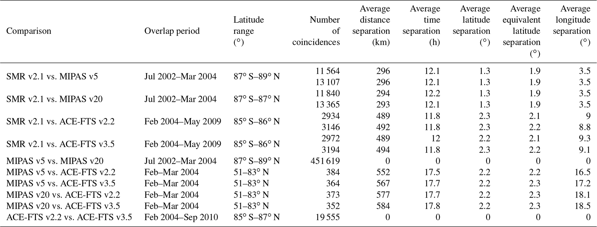
Table 2 Overview of the profile-to-profile comparisons and their coincidence characteristics. For comparisons to the SMR data set the characteristics vary slightly depending upon if the comparison considers HDO (upper row) or H₂O (lower row). The determination of the overlap period and latitude range uses the data from both data sets.

3.1 Profile-to-profile comparisons

3.1.1 Coincidences

In the profile-to-profile comparisons, we generally consider observations from two data sets as coincident when they meet the following criteria: (1) a spatial separation of less than 1000 km, (2) a temporal separation that does not exceed 24 h, and a separation of less than 5^∘ both in (3) geographical and (4) equivalent latitude. In comparisons between the two MIPAS data sets or the two ACE-FTS data sets the exact same observations are used (see Table 2). For the equivalent latitude criterion, we use a stratospheric average value derived from MERRA (Modern-Era Retrospective Analysis for Research and Applications, Rienecker et al., 2011) reanalysis data. In cases where multiple coincidences are found for one observation, the coincidence closest in space is used, given the small local time variation of stratospheric water vapour (Haefele et al., 2008). In the troposphere and higher up in the mesosphere, the variation can be substantial; however, these regions are not the main focus of this study. Additionally, we only consider unique coincidences, i.e. once an observation is considered as a coincidence it is not used any further as coincidence for other observations.

3.1.2 Consideration of differences in the vertical resolution

The vertical resolution of the different HDO and H₂O data sets varies as described in Sect. 2. In particular, the MIPAS HDO and H₂O data sets have a lower vertical resolution than the other data sets. These differences only require consideration in the comparisons at altitudes where the vertical distribution of the parameter in question is highly structured. This especially concerns the hygropause region in the lowermost stratosphere. The maximum of HDO and H₂O around the stratopause is relatively broad. This makes differences in the vertical resolution a smaller issue than for the hygropause region, yet a direct comparison may still not be appropriate.

The differences in the vertical resolution in the HDO and H₂O comparisons to MIPAS are accounted for by the method from Connor et al. (1994). Using the averaging kernel A and the a priori profile x_a priori from the MIPAS retrieval, the higher vertically resolved SMR and ACE-FTS data (x_high) can be degraded onto the MIPAS vertical resolution as follows:

$$\begin{array}{}\text{(3)}& {\displaystyle }{\displaystyle }{\mathit{x}}_{\mathrm{deg}}={\mathit{x}}_{\mathrm{a}\mathrm{priori}}+\mathbf{A}\cdot \left({\mathit{x}}_{\mathrm{high}}-{\mathit{x}}_{\mathrm{a}\mathrm{priori}}\right).\end{array}$$

The degraded data x_deg can subsequently be directly compared to the lower resolution MIPAS data. The comparisons between SMR and ACE-FTS are performed directly, as these data sets have a very similar vertical resolution in the altitude range where they overlap.

Furthermore, δD shows pronounced structures in its vertical distribution, for example in the tropopause region (Webster and Heymsfield, 2003; Nassar et al., 2007). Thus, comparisons of individual δD profiles between the MIPAS and ACE-FTS data sets (see Supplement) should again consider the differences in the vertical resolution. In our case the direct application of Eq. (3) is not possible, as δD is not a retrieved quantity for any of the data sets and consequently no averaging kernels exist. Alternatively the vertical resolution differences in HDO and H₂O can be considered prior to the calculation of the individual δD profiles. Another solution is the generation of appropriate kernels using triangle or Gaussian functions (Dupuy et al., 2009; Lossow et al., 2019a); in the Supplement we employ the first alternative.

3.1.3 Bias determination

The bias $\stackrel{\mathrm{‾}}{b}(P$, z) between two coincident data sets for a given parameter P (i.e. HDO, H₂O, or δD) at altitude z is derived as follows:

$$\begin{array}{}\text{(4)}& {\displaystyle }{\displaystyle }\stackrel{\mathrm{‾}}{b}(P,z)={\displaystyle \frac{\mathrm{1}}{n_{\mathrm{c}}(P,z)}}\cdot \sum _{i=\mathrm{1}}^{n_{\mathrm{c}}(P,z)}{b}_{\mathrm{i}}(P,z).\end{array}$$

In the above equation n_c(P, z) represents the number of coincident measurements and b_i(P, z) denotes the individual differences between them. We have considered these differences in absolute terms:

$$\begin{array}{}\text{(5)}& {\displaystyle }{\displaystyle }{b}_{\mathrm{i}}(P,z)=b_{\mathrm{i},\mathrm{abs}}(P,z)=x_{\mathrm{i}}(P,z{)}_{\mathrm{1}}-x_{\mathrm{i}}(P,z{)}_{\mathrm{2}}\end{array}$$

and also in relative terms:

$$\begin{array}{}\text{(6)}& {\displaystyle }{\displaystyle }{b}_{\mathrm{i}}(P,z)=b_{\mathrm{i},\mathrm{rel}}(P,z)={\displaystyle \frac{x_{\mathrm{i}}(P,z{)}_{\mathrm{1}}-x_{\mathrm{i}}(P,z{)}_{\mathrm{2}}}{\left[x_{\mathrm{i}}(P,z{)}_{\mathrm{1}}+x_{\mathrm{i}}(P,z{)}_{\mathrm{2}}\right]/\mathrm{2}}}.\end{array}$$

x_i(P, z)₁ and x_i(P, z)₂ are the individual observations of the two data sets that are compared with each other. For the relative bias, the average over both data sets is used as a reference. This follows the convenience argument employed by Randall et al. (2003), given the a priori knowledge that the data sets have large uncertainties, especially for HDO and δD.

Before we derive the overall bias $\stackrel{\mathrm{‾}}{b}(P$, z), we perform an additional screening on individual biases b_i(P, z) that are obvious outliers and would skew the bias estimates. This screening employs the median and median absolute deviation (MAD; e.g. Jones et al., 2012), which are more robust quantities in terms of larger outliers. We discarded individual biases that were outside the following interval: $\langle \mathrm{median}\left[b_{\mathrm{i}}\right(P,z\left)\right]\pm \mathrm{10}\cdot \mathrm{MAD}\left[b_{\mathrm{i}}\right(P,z\left)\right]\rangle$ with i=1, …, n_c(P, z). A factor of 10 for the median absolute deviation corresponds to a factor of about 7.5 for the standard deviation considering a normally distributed set of data. Thus, the screening is relatively weak and aims to detect the most prominent outliers.

For the δD bias, the terminology above only applies to the individual approach, for which results are shown in the Supplement. In the separate approach, we first calculate average profiles of HDO and H₂O (again described by P) for each data set separately from the coincident set of data:

$$\begin{array}{}\text{(7)}& {\displaystyle }{\displaystyle }\stackrel{\mathrm{‾}}{x}(P,z)={\displaystyle \frac{\mathrm{1}}{n_{\mathrm{c}}(P,z)}}\cdot \sum _{i=\mathrm{1}}^{n_{\mathrm{c}}(P,z)}{x}_{\mathrm{i}}(P,z).\end{array}$$

In this step we consider exactly the same data points of the data sets that are compared for a given parameter, i.e. if a data point does not exist in one data set (due to missing coverage or screening) the corresponding data point in the other data set is also not considered. The average HDO and H₂O profiles of a given data set are subsequently combined to an average δD profile, following Eq. (1):

$$\begin{array}{}\text{(8)}& {\displaystyle }{\displaystyle }\stackrel{\mathrm{‾}}{x}(\mathit{\delta }\mathrm{D},z)=\left[{\displaystyle \frac{\stackrel{\mathrm{‾}}{x}(\mathrm{HDO},z)}{\mathrm{2}\cdot \mathrm{VSMOW}\cdot \stackrel{\mathrm{‾}}{x}\left({\mathrm{H}}_{\mathrm{2}}\mathrm{O},z\right)}}-\mathrm{1}\right]\cdot \mathrm{1000}.\end{array}$$

The absolute δD bias between two coincident data sets is then calculated as

$$\begin{array}{}\text{(9)}& {\displaystyle }{\displaystyle }\stackrel{\mathrm{‾}}{b}(\mathit{\delta }\mathrm{D},z)=\stackrel{\mathrm{‾}}{x}(\mathit{\delta }\mathrm{D},z{)}_{\mathrm{1}}-\stackrel{\mathrm{‾}}{x}(\mathit{\delta }\mathrm{D},z{)}_{\mathrm{2}}.\end{array}$$

For the relative bias, we follow the approach outlined in Eq. (6):

$$\begin{array}{}\text{(10)}& {\displaystyle }{\displaystyle }\stackrel{\mathrm{‾}}{b}(\mathit{\delta }\mathrm{D},z)={\displaystyle \frac{\stackrel{\mathrm{‾}}{x}(\mathit{\delta }\mathrm{D},z{)}_{\mathrm{1}}-\stackrel{\mathrm{‾}}{x}(\mathit{\delta }\mathrm{D},z{)}_{\mathrm{2}}}{\left[\stackrel{\mathrm{‾}}{x}(\mathit{\delta }\mathrm{D},z{)}_{\mathrm{1}}+\stackrel{\mathrm{‾}}{x}(\mathit{\delta }\mathrm{D},z{)}_{\mathrm{2}}\right]/\mathrm{2}}}.\end{array}$$

3.1.4 More considerations

The results we present for the profile-to-profile comparisons are based on all available coincidences. No separation into specific seasons or latitude bands has been considered, thus neglecting these dependencies in Eqs. (4) to (10). Furthermore, only biases that are based on at least 20 coincident observations are taken into consideration to avoid spurious results. This mostly concerns the lower and upper altitude boundaries where comparisons are possible.

3.2 Comparisons of seasonally averaged latitude cross sections

3.2.1 Data binning

To provide an overview of how the data sets compare as function of time and space, we consider latitude cross sections for different seasons. Accordingly, we average the complete data sets for a given parameter for all seasons (i.e. MAM, JJA, SON, and DJF, represented by t) and latitude bins ϕ of 10^∘ (centred at 85, 75^∘ S, …, 75, and 85^∘ N):

$$\begin{array}{}\text{(11)}& {\displaystyle }{\displaystyle }\stackrel{\mathrm{‾}}{s}(P,t,\mathit{\varphi },z)={\displaystyle \frac{\mathrm{1}}{n_{\mathrm{o}}(P,t,\mathit{\varphi },z)}}\cdot \sum _{i=\mathrm{1}}^{n_{\mathrm{o}}(P,t,\mathit{\varphi },z)}{x}_{\mathrm{i}}(P,t,\mathit{\varphi },z).\end{array}$$

Here, n_o(P, t, ϕ, z) describes the total number of observations x_i(P, t, ϕ, z) that fall into a specific bin. Before these data are averaged, they are screened – again using the median and median absolute difference. Here we use the interval $\langle \mathrm{median}\left[x_{\mathrm{i}}\right(P,t,\mathit{\varphi },z\left)\right]\pm \mathrm{7.5}\cdot \mathrm{MAD}\left[x_{\mathrm{i}}\right(P,t,\mathit{\varphi },z\left)\right]\rangle$ with i=1, …, n_o(P, t, ϕ, z). This screening is a bit more strict than for the profile-to-profile comparisons, as typically less data fall into individual bins. Besides the average, we also calculate the corresponding standard error ϵ(P, t, ϕ, z):

$$\begin{array}{ll}{\displaystyle }& {\displaystyle }\mathit{ϵ}(P,t,\mathit{\varphi },z)=\\ \text{(12)}& {\displaystyle }& {\displaystyle }\sqrt{{\displaystyle \frac{\mathrm{1}}{n_{\mathrm{o}}(P,t,\mathit{\varphi },z)\cdot \left[n_{\mathrm{o}}(P,t,\mathit{\varphi },z)-\mathrm{1}\right]}}\cdot \sum _{i=\mathrm{1}}^{n_{\mathrm{o}}(P,t,\mathit{\varphi },z)}{\left[x_{\mathrm{i}}(P,t,\mathit{\varphi },z)-\stackrel{\mathrm{‾}}{s}(P,t,\mathit{\varphi },z)\right]}^{\mathrm{2}}}.\end{array}$$

Averages that are based on fewer than 20 individual observations or are less than its associated standard error in absolute terms are not considered any further.

Within the separate framework, the seasonally averaged latitude cross sections for δD are calculated from the corresponding results of HDO and H₂O:

$$\begin{array}{}\text{(13)}& {\displaystyle }{\displaystyle }\stackrel{\mathrm{‾}}{s}(\mathit{\delta }\mathrm{D},t,\mathit{\varphi },z)=\left[{\displaystyle \frac{\stackrel{\mathrm{‾}}{s}(\mathrm{HDO},t,\mathit{\varphi },z)}{\mathrm{2}\cdot \mathrm{VSMOW}\cdot \stackrel{\mathrm{‾}}{s}\left({\mathrm{H}}_{\mathrm{2}}\mathrm{O},t,\mathit{\varphi },z\right)}}-\mathrm{1}\right]\cdot \mathrm{1000}.\end{array}$$

The corresponding standard error is calculated according to the Gaussian error propagation:

$$\begin{array}{ll}{\displaystyle }& {\displaystyle }\mathit{ϵ}(\mathit{\delta }\mathrm{D},t,\mathit{\varphi },z)={\displaystyle \frac{\mathrm{500}}{\mathrm{VSMOW}}}\\ \text{(14)}& {\displaystyle }& {\displaystyle }\cdot \sqrt{{\left[{\displaystyle \frac{\mathit{ϵ}(\mathrm{HDO},t,\mathit{\varphi },z)}{\stackrel{\mathrm{‾}}{s}({\mathrm{H}}_{\mathrm{2}}\mathrm{O},t,\mathit{\varphi },z)}}\right]}^{\mathrm{2}}+{\left[{\displaystyle \frac{\stackrel{\mathrm{‾}}{s}(\mathrm{HDO},t,\mathit{\varphi },z)\cdot \mathit{ϵ}\left({\mathrm{H}}_{\mathrm{2}}\mathrm{O},t,\mathit{\varphi },z\right)}{\stackrel{\mathrm{‾}}{s}{\left({\mathrm{H}}_{\mathrm{2}}\mathrm{O},t,\mathit{\varphi },z\right)}^{\mathrm{2}}}}\right]}^{\mathrm{2}}}.\end{array}$$

Given that this information is not available from all data sets, this calculation assumes no error covariance between the HDO and H₂O data to keep consistency.

3.2.2 Summarising the results

For a summary of these comparisons, we provide some additional quantities by combining the results from all individual latitude bands. Results from at least six latitude bands are required, otherwise the combined quantity is discarded. As a first quantity, we consider the average bias ${\stackrel{\mathrm{‾}}{b}}_{\mathit{\varphi }}(P$, t, z) of the latitude cross sections from two data sets:

$$\begin{array}{ll}{\displaystyle }{\stackrel{\mathrm{‾}}{b}}_{\mathit{\varphi }}(P,t,z)& {\displaystyle }={\displaystyle \frac{\mathrm{1}}{n_{\mathit{\varphi }}(P,t,z)}}\cdot \sum _{i=\mathrm{1}}^{n_{\mathit{\varphi }}(P,t,z)}\left[\stackrel{\mathrm{‾}}{s}{\left(P,t,{\mathit{\varphi }}_{\mathrm{i}},z\right)}_{\mathrm{1}}\right.\\ \text{(15)}& {\displaystyle }& {\displaystyle }\left.-\stackrel{\mathrm{‾}}{s}{\left(P,t,{\mathit{\varphi }}_i,z\right)}_{\mathrm{2}}\right].\end{array}$$

The subscripts at the end of the variables refer to the two data sets. In addition to the average, we also look at the de-biased standard deviation:

$$\begin{array}{ll}{\displaystyle }& {\displaystyle }{\mathit{\sigma }}_{\mathit{\varphi }}(P,t,z)=\\ \text{(16)}& {\displaystyle }& {\displaystyle }\sqrt{{\displaystyle \frac{\mathrm{1}}{n_{\mathit{\varphi }}(P,t,z)-\mathrm{1}}}\cdot \sum _{i=\mathrm{1}}^{n_{\mathit{\varphi }}(P,t,z)}{\left[\stackrel{\mathrm{‾}}{s}{\left(P,t,{\mathit{\varphi }}_i,z\right)}_{\mathrm{1}}-\stackrel{\mathrm{‾}}{s}{\left(P,t,{\mathit{\varphi }}_{\mathrm{i}},z\right)}_{\mathrm{2}}-{\stackrel{\mathrm{‾}}{b}}_{\mathit{\varphi }}(P,t,z)\right]}^{\mathrm{2}}}.\end{array}$$

The de-biased standard deviation is generally interpreted as a measure of the combined precision of the two data sets that are compared (von Clarmann, 2006). In this specific case, it describes the combined precision of the seasonally averaged latitude cross section from two data sets. As a last step, we consider the correlation coefficient r_ϕ(P, t, z) between the latitudinal cross sections from two data sets:

$$\begin{array}{ll}{\displaystyle }& {\displaystyle }{r}_{\mathit{\varphi }}(P,t,z)=\\ \text{(17)}& {\displaystyle }& {\displaystyle \frac{\sum _{i=\mathrm{1}}^{n_{\mathit{\varphi }}(P,t,z)}\left[\stackrel{\mathrm{‾}}{s}{\left(P,t,{\mathit{\varphi }}_{\mathrm{i}},z\right)}_{\mathrm{1}}-{\stackrel{\mathrm{‾}}{s}}_{\mathit{\varphi }}(P,t,z{)}_{\mathrm{1}}\right]\cdot \left[\stackrel{\mathrm{‾}}{s}{\left(P,t,{\mathit{\varphi }}_{\mathrm{i}},z\right)}_{\mathrm{2}}-{\stackrel{\mathrm{‾}}{s}}_{\mathit{\varphi }}(P,t,z{)}_{\mathrm{2}}\right]}{\sqrt{\sum _{i=\mathrm{1}}^{n_{\mathit{\varphi }}(P,t,z)}{\left[\stackrel{\mathrm{‾}}{s}{\left(P,t,{\mathit{\varphi }}_{\mathrm{i}},z\right)}_{\mathrm{1}}-{\stackrel{\mathrm{‾}}{s}}_{\mathit{\varphi }}(P,t,z{)}_{\mathrm{1}}\right]}^{\mathrm{2}}}\cdot \sqrt{\sum _{i=\mathrm{1}}^{n_{\mathit{\varphi }}(P,t,z)}{\left[\stackrel{\mathrm{‾}}{s}{\left(P,t,{\mathit{\varphi }}_{\mathrm{i}},z\right)}_{\mathrm{2}}-{\stackrel{\mathrm{‾}}{s}}_{\mathit{\varphi }}(P,t,z{)}_{\mathrm{2}}\right]}^{\mathrm{2}}}}}\end{array}$$

with

$$\begin{array}{}\text{(18)}& {\displaystyle }& {\displaystyle }{\stackrel{\mathrm{‾}}{s}}_{\mathit{\varphi }}(P,t,z{)}_{\mathrm{1}}={\displaystyle \frac{\mathrm{1}}{n_{\mathit{\varphi }}(P,t,z)}}\cdot \sum _{i=\mathrm{1}}^{n_{\mathit{\varphi }}(P,t,z)}\stackrel{\mathrm{‾}}{s}{\left(P,t,{\mathit{\varphi }}_{\mathrm{i}},z\right)}_{\mathrm{1}}\text{and}\text{(19)}& {\displaystyle }& {\displaystyle }{\stackrel{\mathrm{‾}}{s}}_{\mathit{\varphi }}(P,t,z{)}_{\mathrm{2}}={\displaystyle \frac{\mathrm{1}}{n_{\mathit{\varphi }}(P,t,z)}}\cdot \sum _{i=\mathrm{1}}^{n_{\mathit{\varphi }}(P,t,z)}\stackrel{\mathrm{‾}}{s}{\left(P,t,{\mathit{\varphi }}_{\mathrm{i}},z\right)}_{\mathrm{2}},\end{array}$$

which is the average of the seasonally averaged latitude cross section over all latitude bins. No error estimates are considered in the calculation of the correlation coefficient, as the latitudinal cross sections from the two data sets are expected to be highly correlated and not simply correlated by chance.

3.2.3 More considerations

These comparisons do not take the differences in the vertical resolution between MIPAS and the other data sets into account. Obtaining the convolution data to adapt to the vertical resolution of non-coincident data sets is not a trivial procedure. Risi et al. (2012) and Schieferdecker (2015) describe methods for doing so. As the data averaging tends to reduce differences in the vertical resolution, we decided not to consider this aspect any further.

3.3 Comparisons of monthly averaged profiles in the tropics

In the final comparison we consider the tropics, a key region in particular for lower stratospheric water vapour. We focus on February, April, August, and October which are the months the ACE-FTS observations typically provide tropical coverage. In recent years, there has also been some very limited coverage in May and November due to the shift of the SCISAT orbit, but these months are not considered here. The calculation of the monthly averaged profiles follows the same scheme as outlined by Eqs. (11) to (14), except that only one latitude bin (15^∘ S–15^∘ N) is considered and the seasonal dependence is replaced by a monthly dependence. Screening before and after the average calculation is the same as that used for the seasonally averaged latitude cross sections (see Sect. 3.2). Again, no degradation of the ACE-FTS and SMR data sets onto the vertical resolution of the MIPAS data set is considered.

4 Results

4.1 Profile-to-profile comparison

In Fig. 1 we show an example of the absolute δD (upper row), HDO (middle row), and H₂O (bottom row) profiles from the coincident SMR and ACE-FTS v3.5 data sets derived according to Eqs. (7) and (8). In the lower stratosphere the SMR δD values reach −750 ‰, whereas the values in the ACE-FTS profile only reach −550 ‰. As the ACE-FTS values are in the range of expected δD values in the lower stratosphere (Moyer et al., 1996; Johnson et al., 2001; Nassar et al., 2007), the SMR values seem to be too low. A separate consideration of the profiles with regard to the processes contributing to the transport of water vapour into the stratosphere would yield different conclusions. The values of the SMR profile would indicate a larger contribution from slow ascent, whereas the ACE-FTS profile would indicate a larger influence from ice-lofting related to convective processes. With increasing altitude, the bias between the data sets become smaller. The different gradients in δD suggest a different interpretation of the contribution from methane oxidation. Close to 1 hPa the agreement between the two data sets looks quite good; however, this is for the wrong reason, as there are large biases in both HDO and H₂O. Over the entire altitude range we find a more or less constant bias in HDO, whereas the agreement becomes better with decreasing altitude in H₂O. In the lower stratosphere the biases in δD arise from the biases in HDO. The corresponding figures for the comparisons of the other data sets are provided in the Supplement.

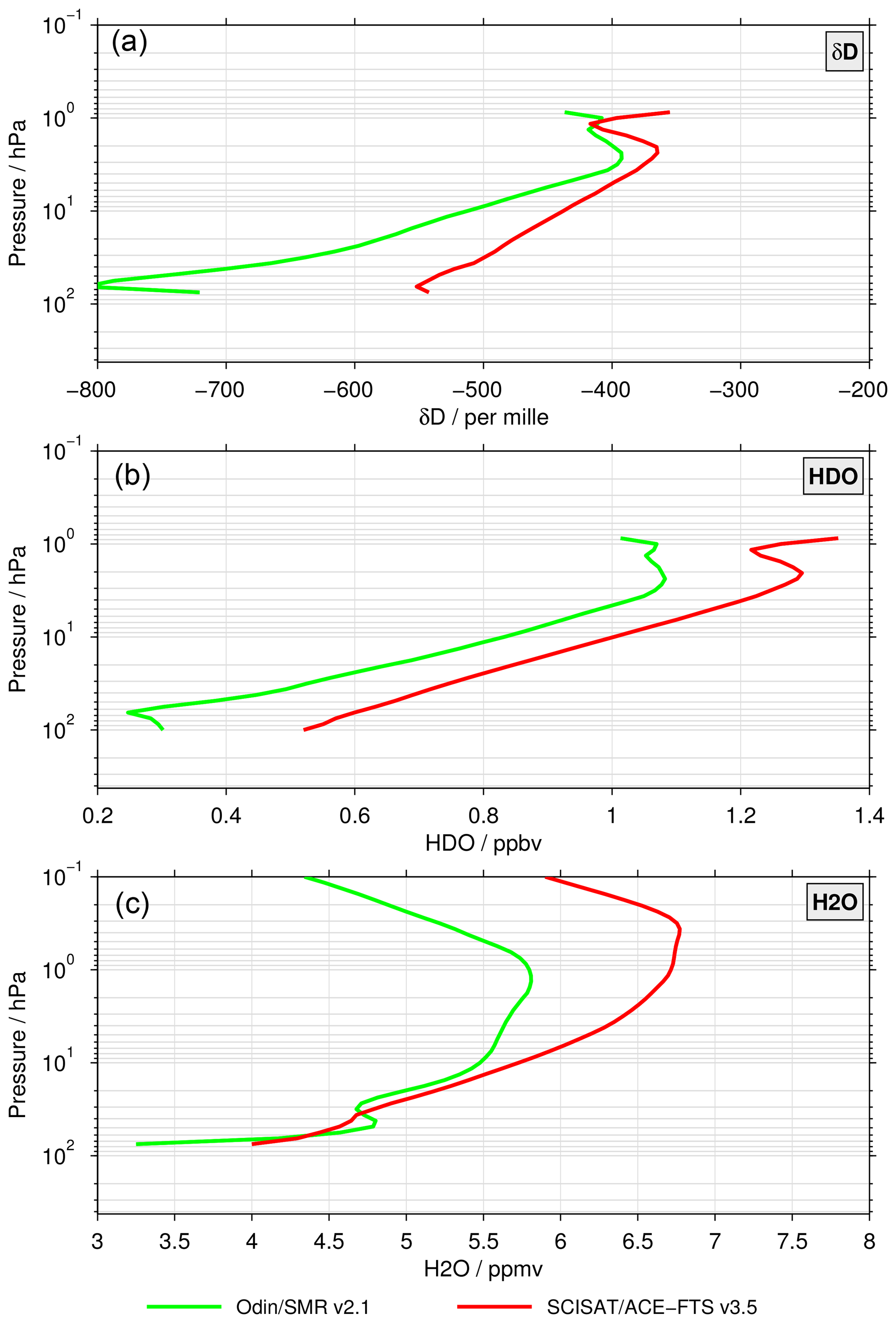
Figure 1 Profile-to-profile comparisons between the SMR v2.1 and ACE-FTS v3.5 data sets considering absolute profiles of δD (a), HDO (b), and H₂O (c).

In contrast, in Fig. 2, the biases derived from the profile-to-profile comparisons (according to the description in Sect. 3.1) are shown, considering all data set combinations. The upper row shows the results for δD, in the middle row the HDO results are considered, and in the lower row the focus is on H₂O. In the left panels the absolute biases are shown, whereas the right panels display the relative biases. Table 2 summarises the characteristics of the comparisons between the different data sets in terms of their overlap period, covered latitude range, number of coincidences, and the average separation in time and space.

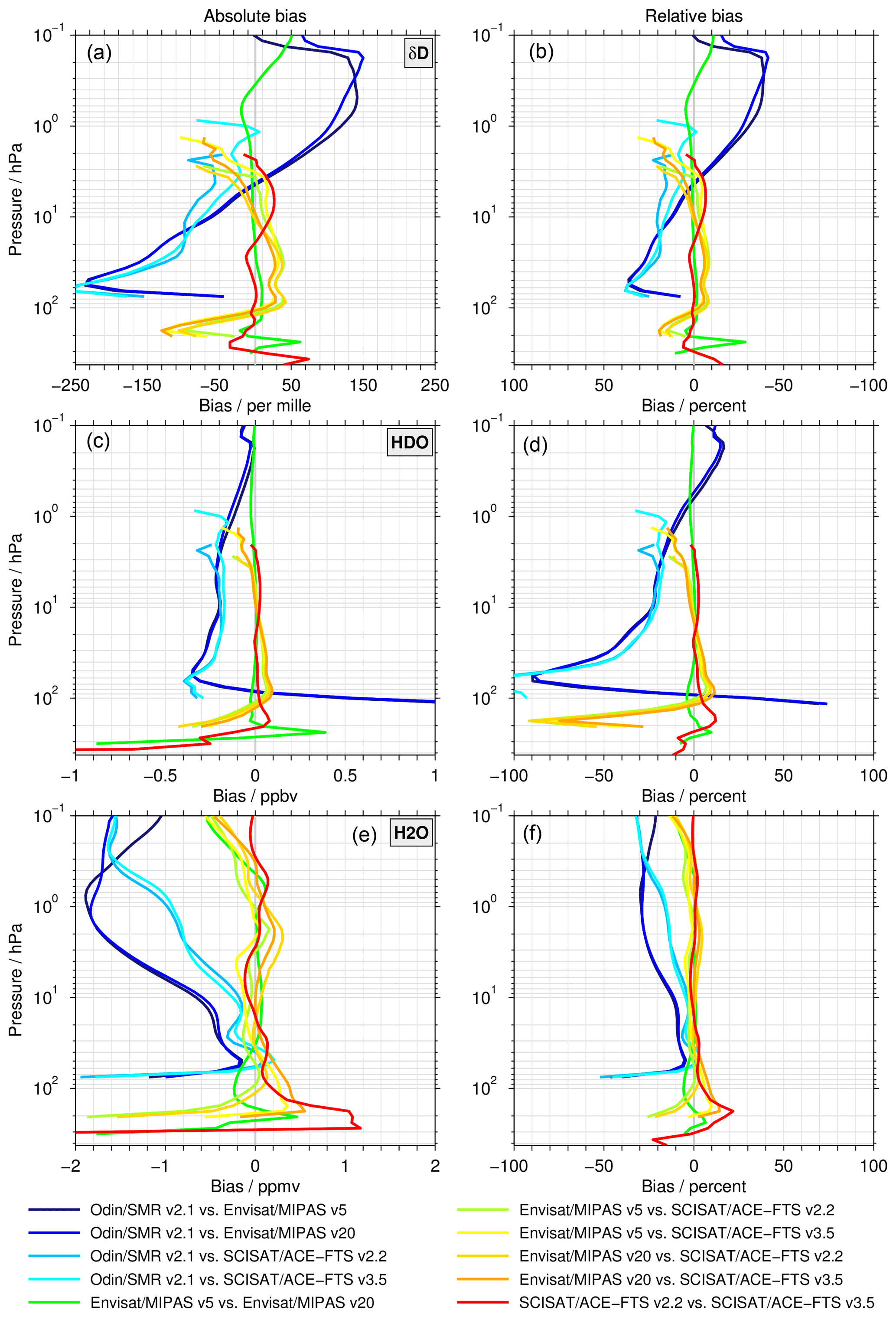
Figure 2 Profile-to-profile comparisons between all data sets for δD (a, b), HDO (c, d), and H₂O (e, f). Panels (a, c, e) show the biases in absolute terms, whereas panels (b, d, f) show the relative biases. Please note that for the relative bias in δD, (b), the x axis has been reversed for visual consistency with the absolute bias.

The comparisons are typically based on several thousand coincidences and cover almost all latitudes and a time period of multiple years. The only exceptions are the comparisons between the MIPAS and ACE-FTS data sets. Given that the MIPAS data sets end in March 2004 and the ACE-FTS observations effectively start in the second half of February 2004, there is only a very limited overlap period. During the short overlap period, the majority of ACE-FTS observations occurred in March at northern polar latitudes. Overall, these comparisons only cover latitudes from 51 to 83^∘ N, and most of the coincidences are concentrated near 70^∘ N. The number of coincident profiles vary between 300 and 400, depending upon which of the MIPAS and ACE-FTS data sets are compared with each other. Also, the average separation in time and longitude are larger for the comparisons between the MIPAS and ACE-FTS data sets than for any of the other comparisons.

The largest deviations in δD are found in the comparisons to the SMR data set. Between the SMR and MIPAS data sets, the absolute bias ranges from −230 ‰ near the 50 hPa region to almost 150 ‰ in the 1 hPa region. In relative terms, the corresponding numbers are 40 % at 100 hPa and −40 % in the stratopause region. The biases change signs slightly below 4 hPa. The comparisons of the SMR data set with the coincident ACE-FTS profiles show similar biases to those described above, with a peak deviation of −250 ‰ around 60 hPa. The biases decrease in size to −100 ‰ at 20 hPa. Above 15 hPa, the biases to the ACE-FTS v3.5 data set are smaller than the bias to the ACE-FTS v2.2 data set. For example, at 4 hPa the biases amount to −55 ‰ (15 %) and −30 ‰ (7 %), respectively. Higher up, the ACE-FTS retrievals come closer to their upper limit and the biases to the SMR data set exhibit distinct variations. The four comparisons between the different MIPAS vs. ACE-FTS data sets generally show good agreement with respect to δD. The biases are typically within ±30 ‰ between about 100 and 4 hPa, corresponding to biases within ±10 % in relative terms. Above and below this altitude range, the biases deteriorate. Comparisons between data sets from the same instrument typically exhibit very small biases. Exceptions primarily occur towards the upper and lower boundaries of the data sets.

Close to 60 hPa, the HDO comparisons to the SMR data set exhibit biases of about −0.4 to −0.3 ppbv (−125 % to −90 %). Towards higher altitudes the biases decrease in size; in the altitude range between 10 and 0.1 hPa, the biases are within ±25 %. The comparisons between the ACE-FTS and MIPAS data sets show good agreement with deviations in the range of ±10% in the lower and middle stratosphere; larger biases are only observed below 100 hPa and above 4 hPa. Furthermore, for H₂O, the comparisons indicate very good agreement between the different MIPAS and ACE-FTS data sets (typically within ±10 %). The comparisons with the SMR data set show the best agreement between about 50 and 10 hPa, where the biases to the MIPAS and ACE-FTS data sets do not exceed −0.5 ppmv (−10 %). Here, the biases are typically larger in the comparison with the MIPAS data sets than with the ACE-FTS data sets. Higher up, the deviations increase to about −25 %. In volume mixing ratio terms, this corresponds to biases of between −2 and −1 ppmv. Again, the size of the deviations is larger in the comparisons with the MIPAS data sets.

4.2 Comparisons of seasonally averaged latitude cross sections

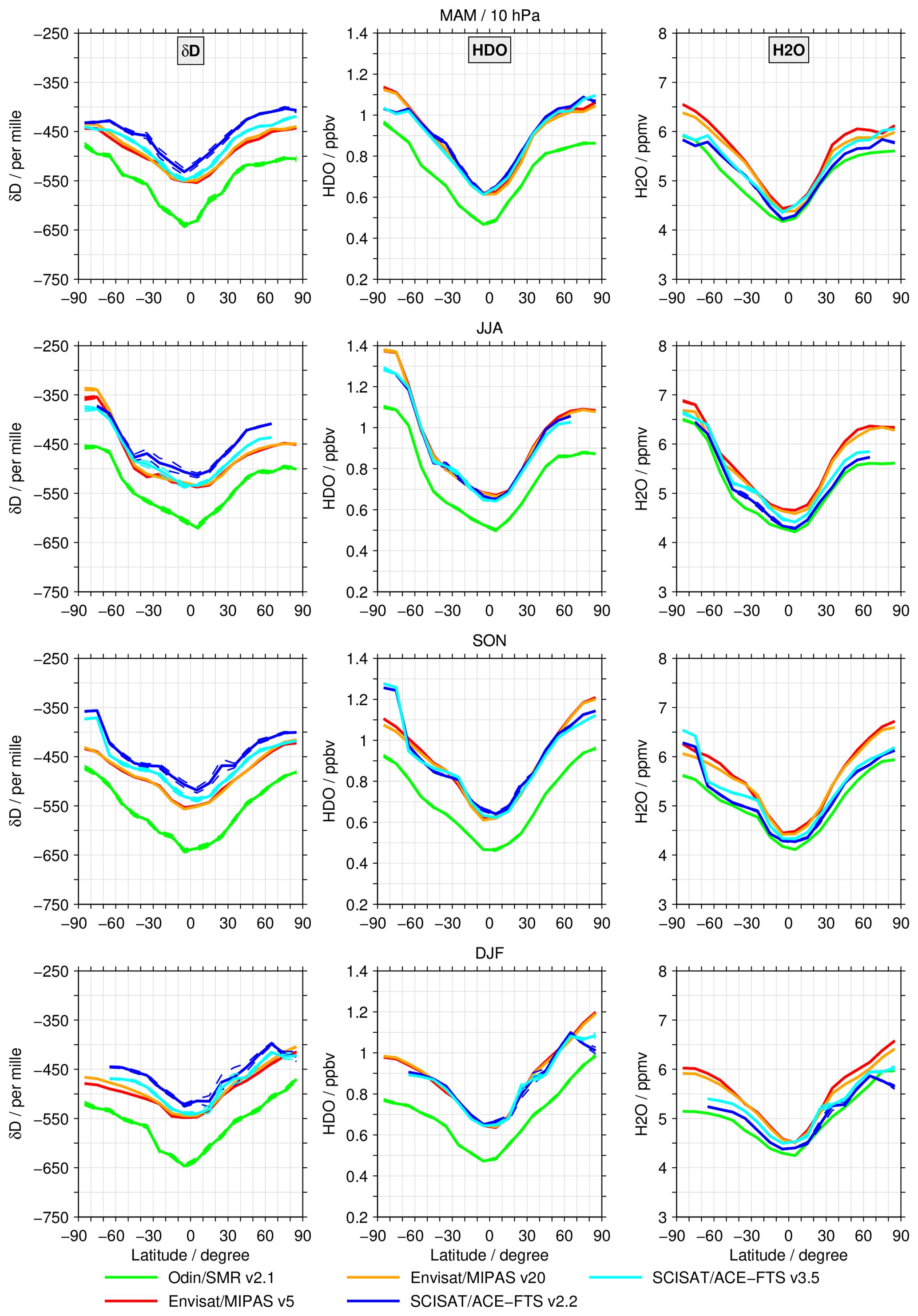
In the following sections, the comparison results from the seasonally averaged latitude cross sections are presented. They aim to provide an overview of how the data sets compare as function of time and space. We start with an overview of all altitudes (Fig. 3) followed by three examples focusing on cross sections at 100, 10, and 1 hPa (Figs. 4 to 6). These three levels have been chosen in order to cover the atmosphere from the tropopause region to the stratopause. Following this, a summary of the results is presented (Figs. 7 to 9), as described in Sect. 3.2.2.

Figure 3 Climatologies of δD for the five data sets considered in this study and for the JJA season.

4.2.1 Examples

All altitudes

Figure 3 shows the latitude–pressure cross sections of δD for JJA for all data sets considered in the comparisons. During this season PSCs occur over the Antarctic and a pronounced latitudinal gradient in δD can be expected due to atmospheric dynamics. On top of the climatological tropopause a large depletion in δD is found in the MIPAS and ACE-FTS data sets, especially in the tropics and Antarctic region. An exception here is the SMR data set which shows the depletion in δD at a higher altitude. As this is the lower limit of the SMR measurements, the structure in δD is not that pronounced and the derived values at these altitudes are more uncertain compared with the MIPAS and ACE-FTS measurements. In the Antarctic, in the PSC areas we expect an influence on δD due to phase transitions related to the formation of ice particles and removal of ice particles through sedimentation at this time of the year. However, the differences found between the MIPAS and ACE-FTS climatologies would lead to different interpretations of the PSC influence on δD. An increase in δD is found with increasing altitude and accompanied by a latitudinal variation. Higher δD values are found over the high latitudes due to “older air” which has had more time for methane oxidation (Stiller et al., 2012; Haenel et al., 2015). Higher δD values are also seen in the Antarctic region in the middle and higher stratosphere due to downwelling of older air within the polar vortex. In the data sets there is a decrease in δD in the lower mesosphere, but with variations between the data sets. Larger differences are seen for the other seasons (see figures in the Supplement). These differences would also lead to different conclusions concerning the processes involved when considering the data sets individually. In the tropical upper troposphere there are large differences related to the lower limit of the MIPAS observations and the influence of clouds. The ACE-FTS data sets most likely show a more realistic, clearer picture of the δD distribution at these altitudes due to the fact that the ACE-FTS instrument can measure at lower altitudes compared with the MIPAS instrument.

100 hPa level

Figure 4 shows the latitudinal cross sections of δD (left column), HDO (centre column), and H₂O (right column) for the 100 hPa level. The different rows consider the results for the different seasons MAM, JJA, SON, and DJF. The dashed lines indicate the standard error of the seasonal averages (see Eqs. 12 and 14). The 100 hPa altitude corresponds to the level of the tropical tropopause where the temperature largely determines the transport rate of water vapour into the stratosphere. Therefore, it is an interesting altitude for comparisons. Both the MIPAS and ACE-FTS data sets cover this altitude, even though it is close to the lower limit of possible retrievals for both instruments. The SMR observations only provide HDO results at this altitude and therefore are not shown in this comparison.

Figure 4 Latitude cross sections at 100 hPa from the different data sets for δD (left column panels), HDO (centre column panels), and H₂O (right column panels) for all seasons (different rows). The thin dashed lines show the standard error of the binned data.

The ACE-FTS data sets typically show the highest depletion in δD in the tropics. The v3.5 data set indicates consistently lower δD values than the v2.2 data set. Towards higher latitudes, the δD values generally increase. A pronounced decrease is observed in the Antarctic in JJA and SON. For the MIPAS data sets, the latitudinal structure in MAM resembles a “W”, with a maximum in the inner tropics and minima at subtropical latitudes. This structure mainly originates from a pronounced deviation in H₂O. Polewards of 60^∘ latitude, the δD values vary less. Similar behaviour is visible in DJF. Unlike in the ACE-FTS data sets, the MIPAS data sets do not show any decrease in the Antarctic in JJA and SON. In both seasons, the MIPAS data sets indicate a maximum in the northern tropics and lower δD values towards the Arctic. In JJA, the δD values derived in the high Antarctic actually indicate the lowest depletion compared with all other latitudes. Overall, deviations of 100 ‰ or more are occasionally observed. For HDO differences are also observed. The latitude dependence of the data sets is more coherent than for δD, with some obvious exceptions observed both in the tropics and the higher latitudes. In JJA and SON, the ACE-FTS data sets also show a distinct drop in the volume mixing ratios polewards of 60^∘ S, which is not captured by the MIPAS data sets. Furthermore, the latitude dependence is generally more consistent among the data sets for H₂O than for δD. The best agreement between the MIPAS and ACE-FTS data sets is found in SON. In particular, the MIPAS v20 data set shows a pronounced deviation at 30^∘ S and 30^∘ N in MAM and DJF. Similar to spikes, the amount of water vapour can be seen to increase prominently by 0.5–1 ppmv in a small latitude range. This clearly influences the latitude dependence observed in δD, resulting in the “W”-shaped latitude dependence described above. A similar, but weaker, behaviour can be observed in the other seasons because the agreement with the other data sets is better, making it less obvious. In DJF, the MIPAS v5 data set shows a pronounced deviation from the ACE-FTS data sets in H₂O in the tropics and subtropics. The differences observed in the Antarctic in JJA and SON for δD and HDO can also be observed in H₂O, but are less pronounced. Be reminded that the MIPAS H₂O data sets included here are specially retrieved versions with a lower vertical resolution adjusted to the HDO resolution, as described in Sect. 2.2.

10 hPa level

At 10 hPa (Fig. 5), in the middle stratosphere, all three satellites provide data for comparisons. The situation is clearly different from that at 100 hPa. The overall latitude dependence in δD is smoother and more evenly distributed compared with 100 hPa. The most pronounced difference in δD is that the SMR data set shows between 50 to 100 ‰ more depletion than the MIPAS and ACE-FTS data sets, with little latitude dependence. In δD, the MIPAS and ACE-FTS data sets exhibit smaller deviations in some regions. Consistently, for all seasons, the ACE-FTS v2.2 data set shows less depletion in δD than the ACE-FTS v3.5 and the two MIPAS data sets for all latitudes and during all seasons. The difference between the ACE-FTS v2.2 and the MIPAS data sets is typically about 25 ‰ in the tropical regions, and often increases somewhat towards the middle latitudes. Poleward of 60^∘ S in SON the ACE-FTS v2.2 and v3.5 data sets show a distinct increase from −450 to −350 ‰. A corresponding feature is also visible in both HDO and H₂O with increases from 1 to 1.25 ppbv and from 5.5 to 6.5 ppmv, respectively. This structure is not apparent in either the MIPAS or the SMR data sets. For HDO, latitude dependence is very consistent among the data sets, as observed for δD. There is again a low bias in the SMR data set, which is approximately 0.15 ppbv and rather independent of season and latitude. In H₂O, a difference such as this is not obvious. Instead, the SMR data set agrees quantitatively rather well with the ACE-FTS data sets. The MIPAS data sets typically exhibit the highest volume mixing ratios. Towards polar latitudes, this high bias often increases, occasionally exceeding 0.5 ppmv. In the tropics, the spread among the data sets roughly varies between 0.2 and 0.5 ppmv.

Figure 5 As for Fig. 4 but considering the 10 hPa level.

Figure 6 As for Figs. 4 and 5 but considering the 1 hPa level.

1 hPa level

In the stratopause region at 1 hPa (Fig. 6), the volume mixing ratio of water vapour in the middle atmosphere reaches its maximum. Data for comparison at this altitude are available from the SMR and MIPAS data sets. The ACE-FTS v3.5 data set has very limited coverage at this altitude level and is thus omitted here. Similar to the previous altitudes, there are pronounced deviations between the data sets. In δD, the sign of the bias between the SMR and MIPAS data sets is reversed compared with the 10 hPa level. The SMR data set typically shows 25 ‰ to 100 ‰ less depletion than the MIPAS data sets. The bias is more dependent on season than latitude. The largest deviations are visible in SON and DJF, whereas in JJA the bias is smallest. In JJA and SON, there is a tendency for the bias to be largest in the Arctic. The MIPAS v20 data set shows consistently larger δD values than the v5 data set, but the deviation is only on the order of a few per mille. The cross sections exhibit similar structures in both HDO and H₂O, but the SMR observations show lower volume mixing ratios than the MIPAS data sets for all seasons and latitudes. In HDO the deviation varies between 0.1 and 0.2 ppbv, whereas for H₂O the deviation varies between 0.7 and 2.0 ppmv. While for HDO the biases only show a small seasonal dependence, the biases in H₂O minimise in JJA. In general, the biases are slightly larger in the polar regions than in the tropics.

4.2.2 Summary of the seasonal comparisons

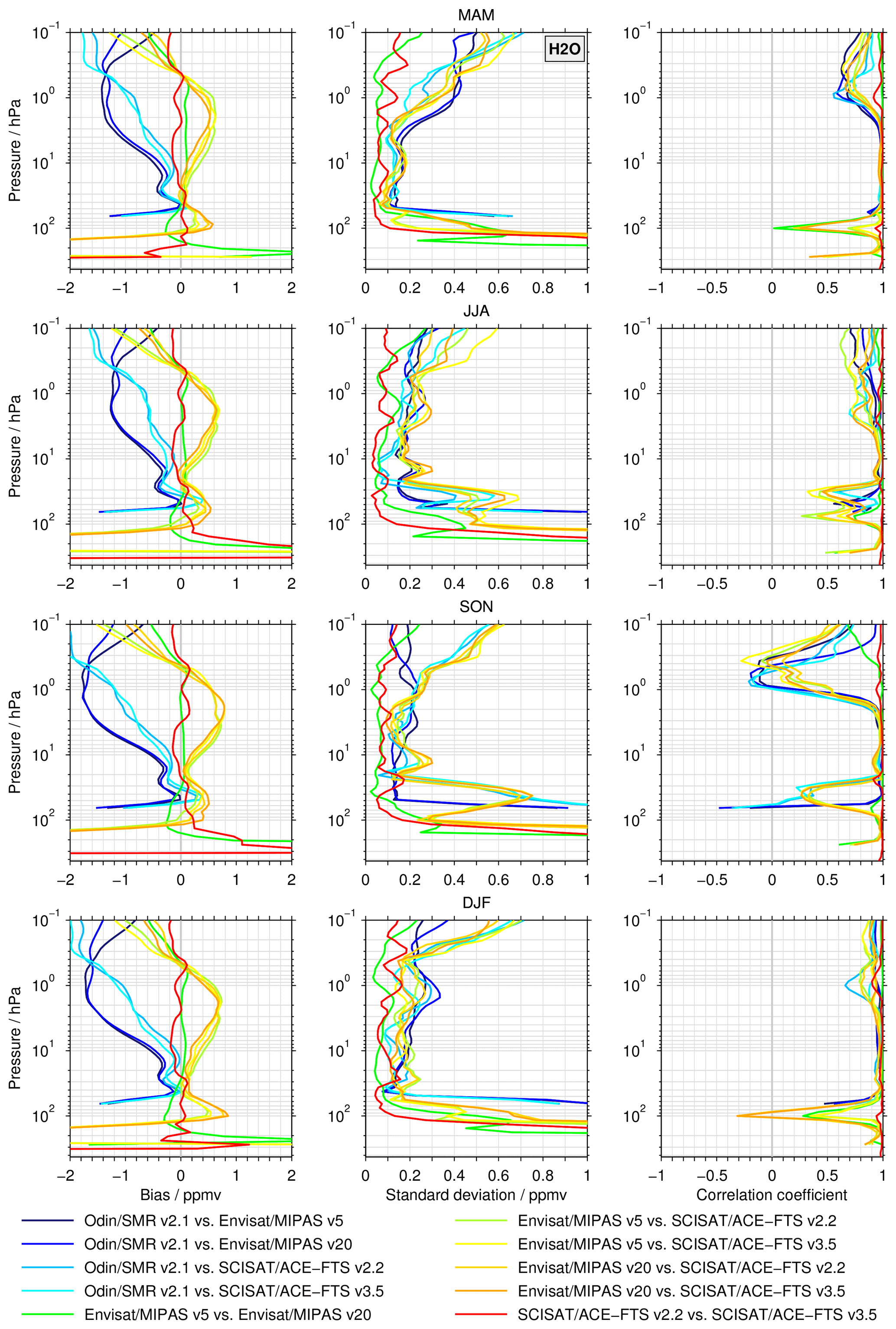
Figures 7 to 9 show summary plots for the comparisons of the seasonal cross sections (see Sect. 3.2.2) that were exemplarily described for the three pressure levels in Figs. 4 to 6. The left column shows the biases between the data sets averaged over all latitudes, the middle column shows the corresponding (de-biased) standard deviations, and the right column shows the correlation coefficients between the cross sections. Figure 7 presents the results for δD, Fig. 8 shows those for HDO, and Fig. 9 displays the results for H₂O. Each figure shows the four different seasons in different rows. The summary figures extend the results obtained from the profile-to-profile comparisons shown in Fig. 2. This is particularly valuable for the comparisons between the MIPAS and ACE-FTS data sets, which were only possible with a very limited temporal and spatial overlap in the profile-to-profile approach.

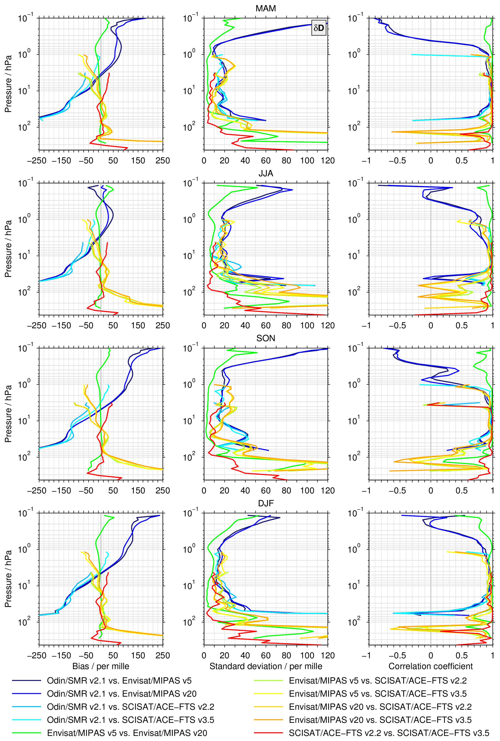
Figure 7 Summary of the seasonal comparisons that were exemplarily shown in Figs. 4 to 6. Here δD is considered. The left panels show the biases averaged over all latitudes for the individual seasons (different rows), the corresponding de-biased standard deviations are shown in the centre panels, and the correlations between the latitudinal cross sections are given in the right panels .

δD

In general, the δD biases among the different data sets averaged over all latitudes (Fig. 7) yield very similar results to those derived from the profile-to-profile comparisons (Fig. 2). Some prominent deviations are visible in the comparisons between the SMR and MIPAS data sets as well as in the comparisons between those from MIPAS and ACE-FTS. For the latter, this primarily concerns altitudes below 100 hPa. The profile-to-profile comparisons in Fig. 2 indicate a low bias of the MIPAS data sets, whereas in Fig. 7 a clear high bias is found. For the comparison between the SMR and MIPAS data sets, the approaches yield differing results at 50 hPa as well as in the upper stratosphere and lower mesosphere. At about 50 hPa, the negative biases are larger than in the profile-to-profile comparisons. The δD bias above 0.3 hPa in Fig. 2 approaches zero, whereas in Fig. 7 the biases continue to increase for all seasons except for JJA. In general, a clear seasonal dependence is observed in the upper stratosphere and lower mesosphere for the comparison between the SMR and MIPAS data sets. At 0.6 hPa, the δD biases are roughly 75 ‰ in MAM while in SON, DJF, and the profile-to-profile comparisons they amount to 125–150 ‰. In JJA, the biases are around 40 ‰. During this season, the bias between the SMR and MIPAS v5 data sets switches signs at about 0.3 hPa; slightly below 0.1 hPa it amounts to about −50 ‰. This behaviour is not observed during other seasons.

The de-biased standard deviations show a characteristic altitude dependence. Between 20 and 0.5 hPa, the deviations are typically smaller than 25 ‰. The lowest values in the comparisons occur between the data sets from the same instrument (typically less than 10 ‰). Below 20 hPa, the standard deviations increase significantly and occasionally exceed 100 ‰ at altitudes lower than 100 hPa. Again, estimates for the comparisons among data sets from the same instrument are smaller, but they are still substantial. Above 0.5 hPa, the comparisons between the SMR and MIPAS data sets also exhibit a pronounced increase in the de-biased standard deviations, maximising in MAM and SON. Values exceeding 100 ‰ are observed close to 0.1 hPa as well. In many ways, the correlation coefficients reflect the behaviour observed for the de-biased standard deviation. Very high correlation coefficients (close to 1) are found between about 20 and 2 hPa. Lower correlations are visible at altitudes where one of the data sets compared reaches one of its vertical boundaries, such as the SMR data set at around 50 hPa, the ACE-FTS v2.2 data set at around 4 hPa (especially in SON), or the ACE-FTS v3.5 data set close to 1 hPa. The comparisons between the MIPAS and ACE-FTS data sets show a distinct reduction of the correlations in a layer around 130 hPa, where the values become negative in all seasons. In the lower mesosphere (above 0.3 hPa), the correlation coefficients between the SMR and MIPAS data sets also become negative.

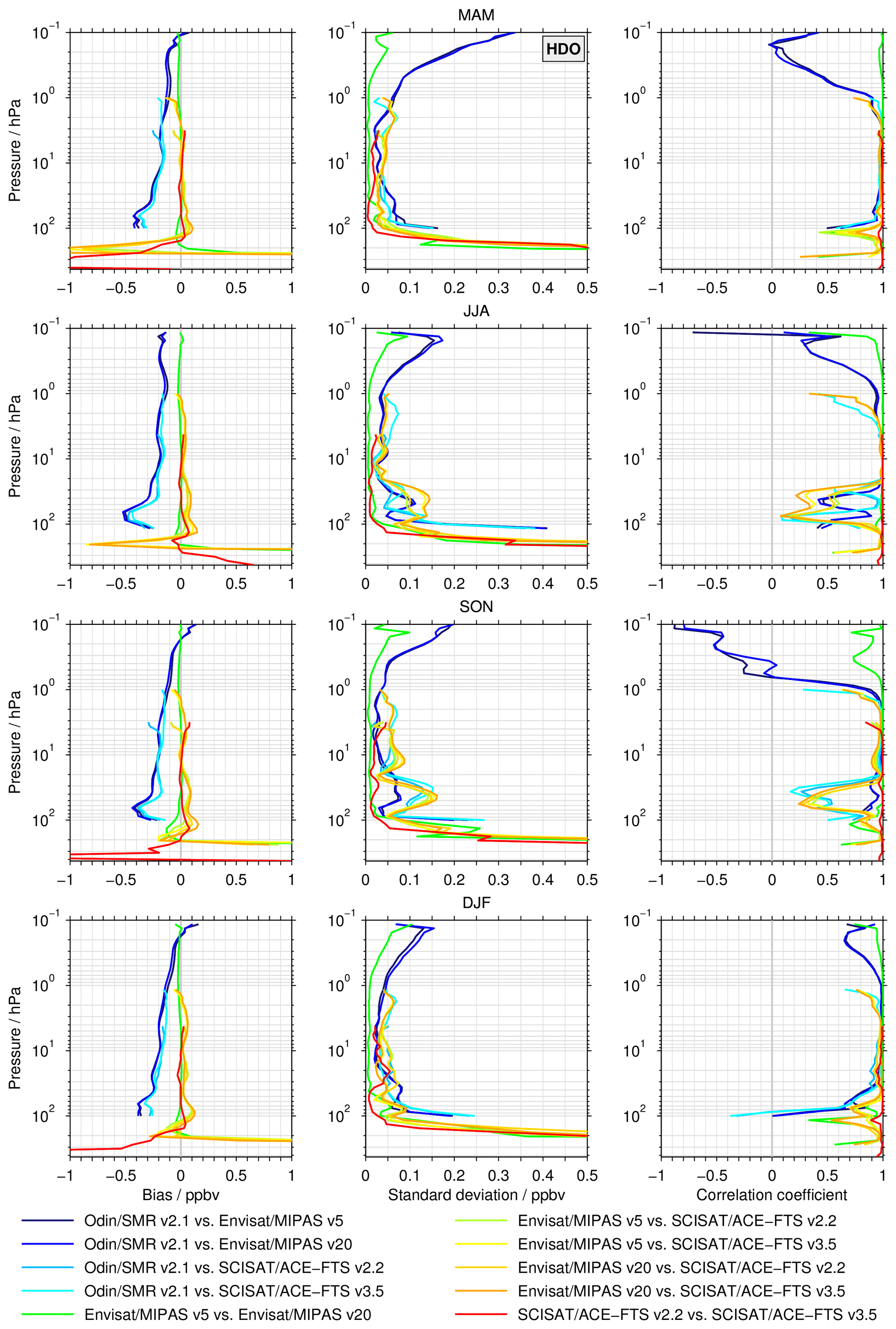
HDO

As for δD, the HDO bias results from the seasonal means averaged over all latitudes (Fig. 8) and the profile-to-profile comparisons (Fig. 2) are quite similar. Differences among these two approaches are again visible below 100 hPa concerning all comparisons. Higher up, above 1 hPa, the biases between the SMR and MIPAS data sets are rather consistent with altitude in JJA, while during the other seasons and in the profile-to-profile comparisons they approach zero. The de-biased standard deviations show similar behaviour, qualitatively, to those from δD. Typically, the values in the middle and upper stratosphere are smaller than 0.07 ppbv. Below this altitude level, the values increase again, in particular below 100 hPa (exceeding 0.5 ppbv). Furthermore, in the lower mesosphere, the comparisons between the SMR and MIPAS data sets exhibit increasing estimates. Close to 0.1 hPa, the standard deviations amount to almost 0.35 ppbv in MAM, 0.2 ppbv in SON, and around 0.15 ppbv in JJA and DJF. The correlation coefficients also show the highest values in the stratosphere, in particular in MAM, where values larger 0.9 are found between 80 and 1.5 hPa. In JJA and SON, a clear reduction (occasionally lower than 0.3) is found between 100 and 30 hPa in most comparisons (except between those data sets from the same instrument). This behaviour coincides with increases in the de-biased standard deviations.

Figure 8 As for Fig. 7 but for HDO.

H₂O

The bias results for H₂O summarised in Fig. 9 resemble those from the profile-to-profile comparison shown in Fig. 2, in a similar to those for δD and HDO. Again, differences are visible below 100 hPa among the two comparison approaches. The comparisons between the MIPAS and ACE-FTS data sets exhibit larger biases around 2 hPa. These biases amount to more than 0.5 ppmv (Fig. 9), whereas they do not exceed 0.3 ppmv in the profile-to-profile comparisons (Fig. 2). The biases relative to the SMR data set show a seasonal variation around 1 hPa, and the smallest estimates are observed in JJA. The de-biased standard deviations are typically smaller than 0.25 ppmv between 20 and 2 hPa. In this altitude range, the values are around 0.1 ppmv for the comparison among the different data sets from the same instrument. Lower down, the de-biased standard deviations increase again. In JJA and SON, a local maximum is observed around 40 hPa, coinciding with a distinct local minimum in the correlation coefficients, which is also observed in the comparisons for HDO. In δD, this behaviour is not as obvious, indicating some cancellation of the problems in HDO and H₂O. At 200 hPa, the de-biased standard deviations exceed 1 ppmv. In the lower mesosphere, the increase is more moderate (up to 0.7 ppmv). The highest correlations in the latitudinal distribution are found in approximately the same altitude region as δD and HDO. A distinct local minimum (with negative values) is observed in SON between 1 and 0.3 hPa. Similarly, a local minimum is found at around 100 hPa in MAM and DJF. Be reminded again that the MIPAS H₂O data sets are based on special retrievals, in contrast to the nominal data sets (see Sect. 2.2).

Figure 9 As for Figs. 7 and 8 but for H₂O.

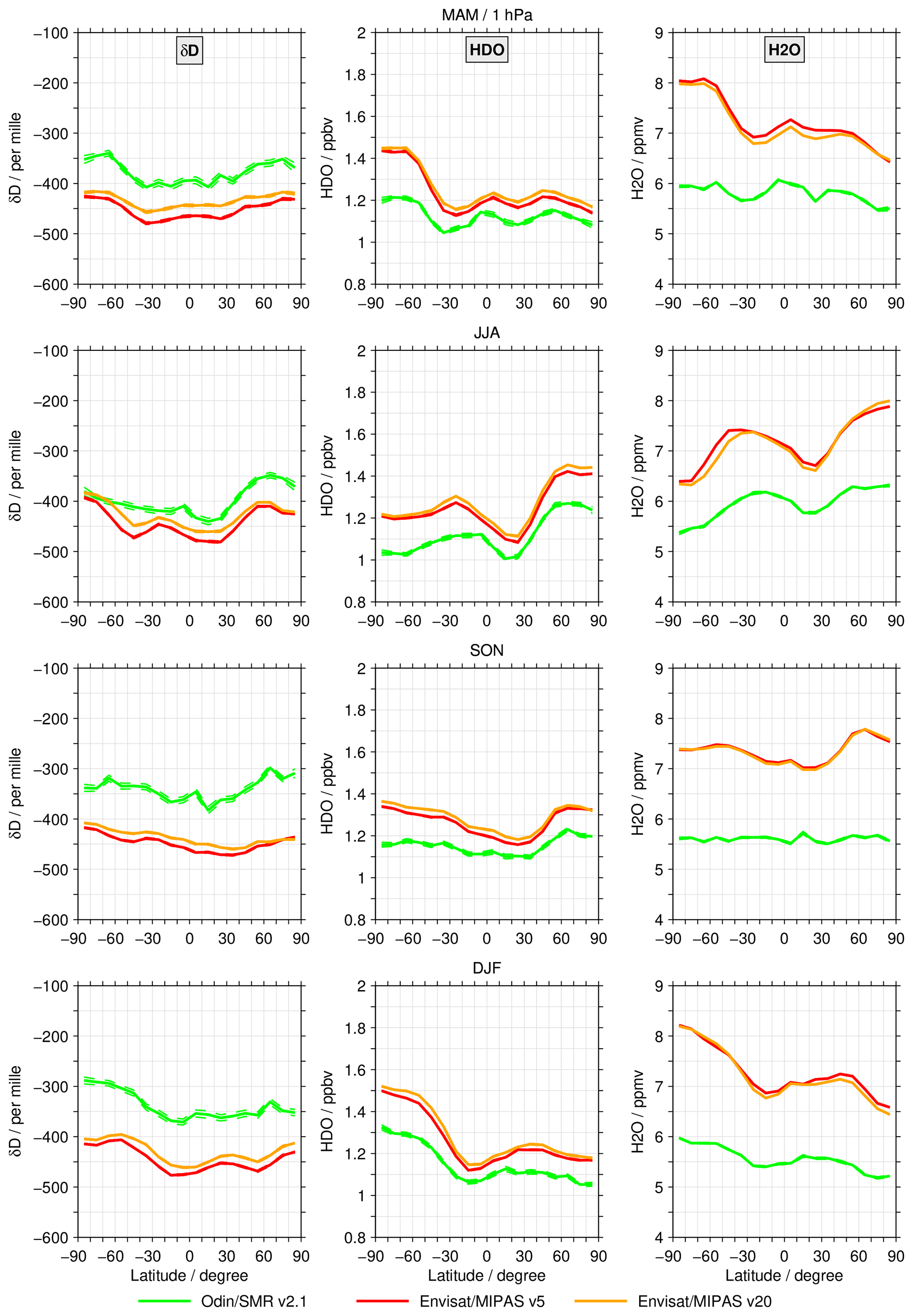
4.3 Monthly averaged profiles in the tropics

Figure 10 shows the tropical (15^∘ S to 15^∘ N) monthly mean profiles of δD (left column), HDO (middle column), and H₂O (right column) for February, April, August, and October (different rows). The ACE-FTS observations, which focus on middle and high latitudes, typically only cover the tropics during these months. For this reason, the monthly averaged data are shown as they give a more appropriate depiction of the isotopic ratio and the corresponding water vapour profiles in this region instead of the seasonal averages used in the previous section. Our primary focus here is on the lower stratosphere. In this region, HDO and H₂O exhibit the tape recorder signal which manifests itself in additional extrema in the vertical distribution above the hygropause. For δD, the existence of a tape recorder is under debate, as described in Sect. 1.

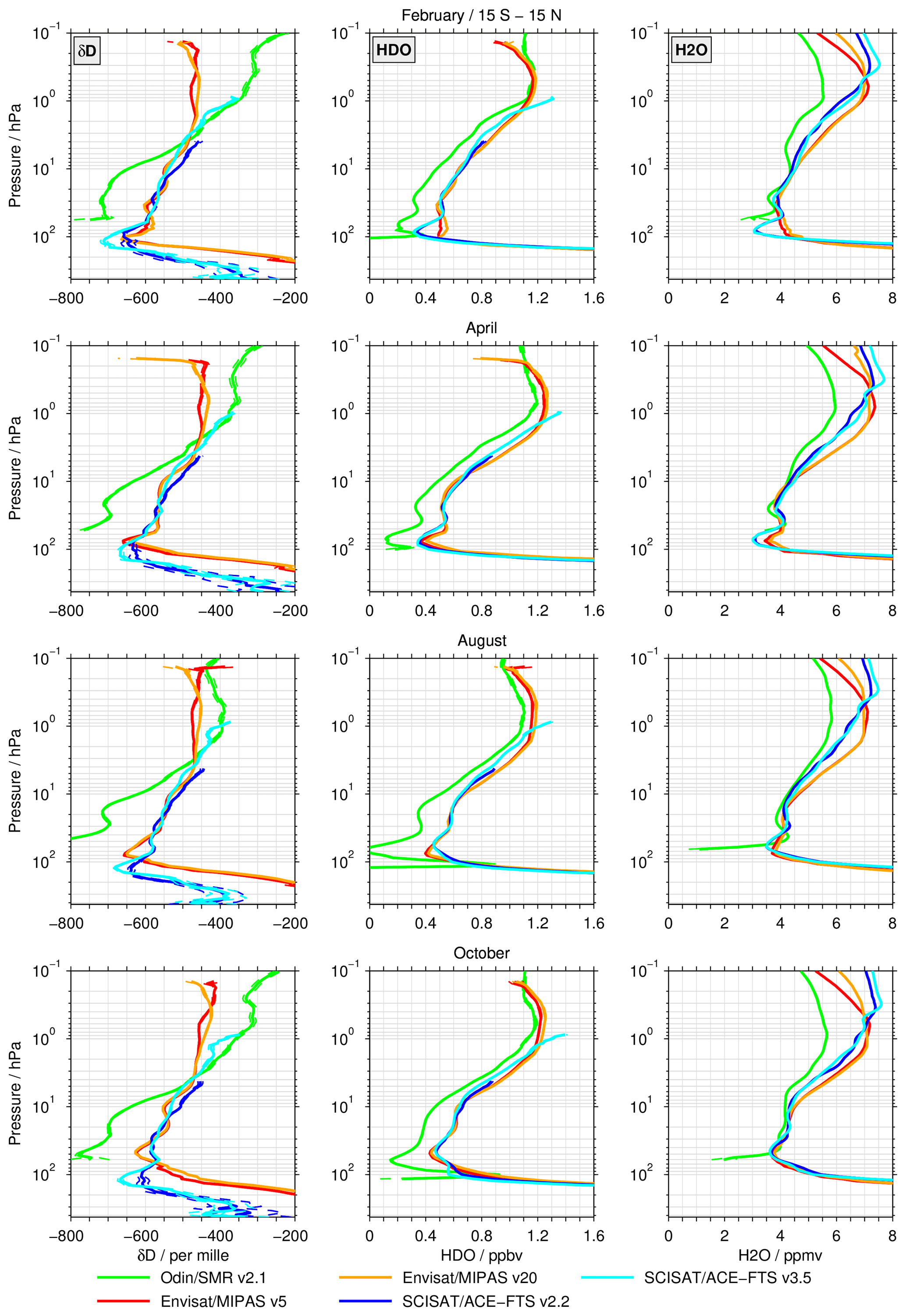
Figure 10 Tropical mean (15^∘ S–15^∘ N) profiles for δD (left column panels), HDO (middle column), and H₂O (right column panels) for February, April, August, and October given in different rows.

Lower stratosphere

In February, both MIPAS data sets capture the tape recorder structure in δD with the first minimum of −670 ‰ near 100 hPa, followed by the maximum of −580 ‰ propagating from the previous season at an altitude of 70 hPa. Above, the corresponding second minima from the previous winter of −600 ‰ at 35 hPa can be seen. However, the MIPAS data sets do not capture the tape recorder structure in the lower stratosphere in the HDO and H₂O data. Instead, the minimum associated with the hygropause is rather wide, due to the rather low vertical resolution in the dry phase of the tape recorder. In δD the ACE-FTS v3.5 shows a clear first minimum of −700 ‰ at an altitude of approximately 100 hPa. This minimum is wider in altitude than for the MIPAS data sets. Higher up there is no tape recorder structure, except a small tendency to another minimum visible around 20 hPa. This is slightly more obvious for the ACE-FTS v2.2 data set, with a weak maximum at about 40 hPa and a second minimum close to 30 hPa. The first minimum around 100 hPa indicates approximately 50 ‰ less depletion than for the v3.5 data set. This behaviour is observed during all of the months considered here. In contrast to the wide minimum observed in the MIPAS data sets, the ACE-FTS HDO and H₂O data sets exhibit a distinct hygropause. A weak local maximum is found close to 50 hPa and a second minimum slightly above 30 hPa, in both the HDO and H₂O data sets. This structure is most pronounced in H₂O for the v3.5 data set. The SMR δD data deviate from the other data sets, in particular in terms of the absolute values. The lower limit of this data set is close to 50 hPa. There, it seems to display the tape recorder maximum (around −700 ‰) and the second minimum is presumably located at 30 hPa (about −720 ‰). As seen in the previous comparisons, the SMR HDO data has a low bias of about 0.2 ppbv relative to the other data sets in the lower stratosphere. At the lower limit, the mixing ratio approaches zero and actually becomes negative. However, the tape recorder structure is clearly visible in these data. The altitudes of the maximum and second minimum are quite similar to those observed in the ACE-FTS data sets. In H₂O, these extrema are located slightly higher than in the ACE-FTS data.

In April, the first δD minimum is clearly located higher in the MIPAS (around 75 hPa) than in the ACE-FTS data sets, which shows this minimum at about the same altitude as in February. The MIPAS data sets show a rather constant isotopic ratio between 50 and 10 hPa. Weak tape recorder structures are visible in the ACE-FTS data sets, but the extrema are located higher in altitude for the v3.5 data set. The SMR data set shows pronounced structures with a maximum slightly below 30 hPa and a minimum at 20 hPa. In HDO and H₂O, the tape recorder structures are clearly visible in all data sets with differences in the absolute mixing ratios and the altitudes of the extrema. In particular, the maximum is located at a lower altitude in the MIPAS data sets (at 50 hPa), whereas in the other data sets the maximum is located at about 40 hPa.

For δD, the situation in August is quite similar to that in April. In HDO, the deviations between the SMR and the other data sets are larger at the hygropause compared with April. Furthermore, the hygropause is higher in altitude in the ACE-FTS than the MIPAS data sets. Likewise, the tape recorder structures in H₂O differ among the data sets. They are most pronounced in the SMR data set, but the maximum occurs at a lower altitude than in the other data sets. The second minimum has its highest location in the ACE-FTS data sets.

There are pronounced differences in δD between the MIPAS and ACE-FTS data sets in October in the lower stratosphere. Both HDO and H₂O differences contribute to the bias in δD. The first minimum is observed at slightly below 100 hPa in the ACE-FTS data sets, whereas it is located much higher, i.e. around 50 hPa, in the MIPAS data sets. Above this altitude level, clear tape recorder structures are visible in all data sets from both instruments, but the shift in altitude remains.

Altitudes above 10 hPa

Focusing on altitudes above 10 hPa, the SMR data set shows lower depletion in δD than the MIPAS data sets above about 3 hPa, as also observed in the seasonal comparisons. The biases vary from month to month and maximise in the lower mesosphere in February. The SMR and ACE-FTS v3.5 data sets show good agreement between 3 and 1 hPa. Good agreement in HDO between the SMR and MIPAS data sets is observed in the altitude range from 1 to 0.2 hPa in February. Above 0.2 hPa, the SMR data set typically shows higher mixing ratios than the MIPAS data sets; elsewhere, the low bias already seen in the previous figures (i.e. Figs. 2 and 8) is also visible. Between 7 and 1.5 hPa the MIPAS data sets show slightly higher HDO volume mixing ratios than the ACE-FTS data sets. At the upper limit of the ACE-FTS v3.5 data set, i.e. close to 0.9 hPa, it shows higher mixing ratios of 0.1 to 0.15 ppbv (largest in February and October) relative to the MIPAS data sets. In terms of H₂O, the data from the three instruments start to deviate above 10 hPa. The lowest mixing ratios are observed for the SMR data set. Up to about 0.5 hPa, the ACE-FTS data sets show lower mixing ratios than the MIPAS data sets (up to 0.75 ppmv), whereas above the altitude the behaviour is reversed. The altitude where the middle atmospheric water vapour maximum is found differs among the data sets from the three instruments. At 0.1 hPa, the MIPAS v5 data set shows a lower H₂O mixing ratio than the v20 data set during all months. Similarly, the ACE-FTS v2.2 data set shows a lower amount of H₂O than the v3.5 data set at this altitude.

5 Discussion and conclusion

We have assessed the quality of satellite δD(H₂O) observations from the upper troposphere to the lower mesosphere using profile-to-profile and climatological comparisons. We find clear quantitative differences in the isotopic ratio. These quantitative differences are largest in comparisons with the SMR data set. The MIPAS and ACE-FTS data sets agree rather well with each other, with exceptions close to the vertical limit where observations can be made by these instruments, i.e. below 100 hPa and in the upper stratosphere.

For the profile-to-profile comparisons (Fig. 2), in the lower stratosphere the SMR data set shows significantly higher δD depletions than the MIPAS and ACE-FTS data sets. However, we note that this is close to the SMR lower limit, which has larger uncertainties. The biases maximise in size close to 50 hPa and exceed −200 ‰. In the upper stratosphere and lower mesosphere the behaviour is reversed, with the SMR data set instead showing less depletion than the MIPAS data sets. The biases switch signs close to 4 hPa. Above this altitude, the biases increase to almost 150 ‰ in the lower mesosphere, where the MIPAS data sets, close to their upper retrieval limit, also arguably become more uncertain. Qualitatively, the same behaviour is observed in the seasonal comparisons (averaged over all latitudes), with some quantitative variations among the seasons, in particular in the lower mesosphere. The δD biases of the SMR data set can be related to biases in both HDO and H₂O.

For HDO, the SMR data set exhibits a low bias (Figs. 2 and 8) throughout all seasons. In the lower stratosphere, the biases are larger than 0.25 ppbv and then decrease with increasing altitude to become close to zero at 0.2 hPa. For H₂O, in comparison, the SMR data set compares rather well to the MIPAS and ACE-FTS data sets in the lower stratosphere (Figs. 2 and 9), whereas in the upper stratosphere and lower mesosphere, distinct low biases are visible. The maximum H₂O bias for the SMR comparisons in the upper stratosphere varies between 1 and 2 ppmv, depending on season. Overall, the δD biases of the SMR data set are driven by HDO in the lower stratosphere, whereas H₂O is the clear driver in the upper stratosphere and lower mesosphere. In between these levels, in the middle stratosphere, the biases in δD are a combination of deviations in both HDO and H₂O. Biases in both HDO and H₂O exist at around 4 hPa where the δD biases of the SMR data set are close to zero compared to the MIPAS and ACE-FTS data sets, because the HDO and H₂O biases cancel each other out.

5.1 SMR results

The biases in the SMR data set can be attributed to both, uncertainties in the spectroscopic parameters used for the retrieval (they are larger than in the infrared region where MIPAS and ACE-FTS perform measurements) and issues in the instrument calibration. In terms of spectroscopic parameters, uncertainties in the line broadening, the temperature dependence exponent, and the line intensity are of interest (Janssen, 1993). As described by Lossow et al. (2011), a 5 % uncertainty in the line broadening parameter of the HDO emission line translates to biases of up to 0.05 ppbv in the retrieved data. For the H₂O emission line the same uncertainty can cause biases in the retrieval results of up to 0.7 ppmv in the lower stratosphere. Around 5 hPa only small biases are visible, whereas in the lower mesosphere the uncertainty amounts to biases between 0.3 and 0.4 ppmv. For δD, the uncertainty of the line broadening parameters, originating from both HDO and H₂O correspond to biases of 30 ‰ in the lower stratosphere and to 60 to 70 ‰ in the lower mesosphere. For the temperature dependence exponent a 10 % uncertainty for the HDO emission line results in biases of 0.01 ppbv in the retrieved results. In terms of H₂O the biases are about 0.1 ppmv, except in the lower stratosphere where they can be as large as 0.2 ppmv. Combining these results for δD yields biases smaller than 20 ‰ for the assumed uncertainty in the temperature dependence exponent. For these two spectroscopic parameters higher uncertainties cannot be ruled out, increasing the bias estimates provided here. With regard to the line intensity, the uncertainty is about 2 % for the HDO and H₂O emission lines. This translates to biases of 0.025 ppbv for HDO and 0.1 ppmv for H₂O. In terms of δD these biases actually cancel out each other.

Issues with instrument calibration primarily relate to the sideband filtering, given that SMR is operated as a single sideband receiver (Frisk et al., 2003; Lossow et al., 2007). If nominal settings were achieved side band leakages smaller than 2 % would be expected. The latest leakage estimates vary up to 5 % and exhibit some time dependence. In principle, the maximum suppression of the sideband filter seems not to have changed significantly. Instead the filter reference length is the largest source of concern. This reference length controls the frequencies at which the sideband filtering is optimal and these frequencies have apparently shifted over time. The uncertainty of the filter reference length is estimated to be 4 µm. For HDO this uncertainty corresponds to biases of up to 0.07 ppbv in the lower stratosphere, which is clearly an important contribution. Higher up, the influence is only 0.01 ppbv. For H₂O the uncertainty of the filter reference length results in biases of up to 1 ppmv in the lower stratosphere. At around 10 hPa the influence is less than 0.2 ppmv but increases above this altitude up to 0.5 ppmv in the lower mesosphere. In terms of δD, the uncertainty of the filter reference length translates to biases of 30 ‰ in the lower stratosphere and 50 ‰ in the lower mesosphere. Around 7 hPa a negligible influence is observed.

The uncertainties in the sideband leakage are associated with the prominent positive drifts which are observed in the SMR H₂O results (Khosrawi et al., 2018). Thus, over time, the low H₂O biases in this altitude range decrease, as do the biases in δD. This has an impact on the results from the profile-to-profile and seasonal comparisons relative to MIPAS. While the profile-to-profile comparisons only cover the years from 2002 to 2004, the climatological comparisons include SMR data until 2009. In MAM and JJA in particular, reduced biases of δD and H₂O are visible in the upper stratosphere and lower mesosphere in the climatological comparisons relative to the profile-to-profile comparisons.

Besides the sideband filtering, there are also uncertainties arising from the autocorrelator calibration. They are part of ongoing studies. Overall, the uncertainties in the spectroscopic parameters and in the instrument calibration have the potential to explain the observed biases of the SMR data. In the lower mesosphere parts of the observed biases may actually be attributed to the MIPAS data sets, which are here also close to the upper vertical limit where retrievals are possible.

5.2 MIPAS and ACE-FTS results

The profile-to-profile comparisons (Fig. 2) between the MIPAS and ACE-FTS data sets exhibit the best agreement in the 100 to 5 hPa region. Most of the time the MIPAS data sets show a small high bias in δD, up to about 25 ‰ (10 %). Furthermore, for the HDO and H₂O data, the agreement in the same altitude region is rather good. However, due to the short overlap time and the small latitude coverage, these results have limited value. The climatological latitude cross sections include the entire data sets and thus allow a more conclusive overview. In these comparisons (Fig. 7), the MIPAS and ACE-FTS δD data sets agree best between 100 and 10 hPa. Even though the biases are low in this region, the de-biased standard deviations roughly amount up to 50 ‰ (larger in JJA). This indicates that there are biases in the latitudinal distribution between the data sets that cancel out in the average. Also, smaller biases exist in HDO (roughly around 0.1 ppbv) and H₂O (up to about 0.5 ppmv, larger in DJF), in particular in the lower part of this altitude range. They partly cancel out each other in the calculation of the δD ratio and in the average over all latitudes, and therefore result in a relatively good agreement in δD.

Above 10 hPa, the δD biases between the MIPAS and ACE-FTS data sets increase, in particular in the comparisons to the ACE-FTS v2.2 data set. Here, the MIPAS data sets show a higher depletion. However, the de-biased standard deviations are relatively low (largely within 20 ‰) and the correlation coefficients are relatively high, indicating only small variations over all latitudes. These δD biases are primarily driven by high biases in the MIPAS H₂O data (up to 0.8 ppmv) peaking at about 2 hPa. Below 100 hPa, the MIPAS and ACE-FTS data sets also show larger deviations. The bias estimates from the seasonal (Fig. 7) and profile-to-profile comparisons (Fig. 2) differ significantly. In the profile-to-profile comparisons, the MIPAS δD data indicate a 100 ‰ (20 %) higher depletion than the ACE-FTS δD close to 200 hPa; in the climatological comparisons, in comparison, the result is the opposite and the MIPAS data sets show significantly less depletion at 200 hPa. In both comparisons the biases are driven by differences in HDO and H₂O. In the profile-to-profile comparisons, the HDO biases are about 0.3–0.4 ppbv (60 %–90 %), for H₂O they are within ±25 % at this altitude. For the climatological comparisons the HDO bias at 200 hPa is in the range of 0.25–1 ppbv depending on season, with the largest bias in MAM and smallest bias in SON and DJF.

The reasons for the biases between the MIPAS and ACE-FTS data sets are manifold: differences in temporal and spatial sampling, cloud influence, vertical resolution, the choice of microwindows and spectroscopic databases, as well as the less-than perfect MIPAS H₂O product used here. This product is retrieved jointly with HDO in the attempt to match the vertical resolution of the latter (see Sect. 2.2). The differences in the temporal and spatial sampling between the MIPAS and ACE-FTS observations can affect the results of climatological comparisons. On the one hand, this concerns the different measurement periods with the MIPAS observations providing data from July 2002 until March 2004 and the ACE-FTS observations starting in February 2004 and lasting for many years.

In this context, changes in variability, like trends, QBO (quasi-biennial oscillation) influence, and the occurrence of sudden stratospheric warmings between these different time periods play a role. For example, according to the SWOOSH (Stratospheric Water and Ozone Satellite Homogenized, Davis et al., 2016) database, H₂O has increased from the MIPAS to the ACE-FTS observation period at almost all latitudes and stratospheric altitudes. This does not help the discussion of biases among the data sets, as the MIPAS data exhibit higher H₂O mixing ratios in most of the stratosphere, in particular around 50 and 2 hPa (Fig. 9). On the other hand, the sampling issue concerns the actual sampling within a given time and latitude bin. The MIPAS satellite utilises a sun-synchronous orbit that provides coverage of almost all latitudes on a daily basis. In contrast, the latitudinal coverage of ACE-FTS observations varies throughout the year. The SCISAT orbit is optimised for high and middle latitudes, yielding the bulk of observations in these regions. In this regard, the MIPAS observations provide a rather complete coverage of the individual seasons in the tropics. For the ACE-FTS orbit, the seasonal means for MAM are based on observations in April, JJA on observations in August, SON on observations in October, and DJF on observations in February, respectively. This may explain some of the tropical biases observed in Figs. 4 and 5 and is more appropriately handled in the monthly comparisons in Sect. 4.3.

Besides the actual sampling, the variability within a given time and latitude bin is also of importance for the sampling bias (Toohey et al., 2013). One prominent example for this is the wintertime lower stratosphere in the Antarctic that is influenced by dehydration induced by PSCs. Such dehydration indications are visible in all data sets in both HDO and H₂O, but with various strengths. It is smallest in the MIPAS data and largest in the ACE-FTS (and SMR) data sets. This behaviour can be explained by sampling biases in combination with large variability. While the MIPAS data cover all of the winter months in the Antarctic, the ACE-FTS coverage depends on the actual month. In June and July, the ACE-FTS observations only reach up to 60 and 70^∘ S, respectively. It is only in August that the observations cover latitudes polewards of 70^∘ S, where the influence of PSCs and the associated dehydration is substantial, leading to a pronounced signal in the seasonal average for the ACE-FTS data sets. The other explanation for the different representation of dehydration in the data sets relates to differences in cloud influence on the MIPAS and ACE-FTS observations, which is actually another aspect of a sampling bias. While the observations of the two instruments are performed in the infrared, they use different measurement techniques. The MIPAS instrument measured thermal emission at the atmospheric limb. The solar occultation technique used by the ACE-FTS instrument provides a stronger signal, which results in a lower sensitivity to cloud presence compared to the MIPAS observations (in comparison, the SMR observations exhibit the smallest cloud influence, as they are performed in the microwave region). In the presence of PSCs, many MIPAS observations actually have to be screened (see Sect. 2.2), weakening the dehydration signal. The other region where these differences in the cloud influence between the MIPAS and ACE-FTS data sets are important is in the troposphere. Again, more MIPAS observations are screened, which can be expected to result in a dry bias. This is observed in H₂O (Fig. 9), but not in HDO (Fig. 8).

In addition to this basic cloud influence, the behaviour of HDO and H₂O differs in the presence of clouds due to differences in the vapour pressure. Consequently, deviations in the depletion can be assumed, given the differences in the cloud influence between the MIPAS and ACE-FTS data sets. For example, if there are no clouds present, the dehydration near the tropical tropopause should reflect more Rayleigh fractionation and result in isotopic ratios close to −900 ‰. In the presence of clouds, the depletion should be lower. Given that the MIPAS data sets represent more cloud-free conditions, a higher depletion relative to the ACE-FTS data sets is expected but not apparent (Fig. 10). This may relate to differences in the vertical resolution among the data sets. As described in Sect. 3.1.2, the differences in the vertical resolution of the MIPAS and ACE-FTS data sets can cause biases if they are not considered as with the climatological comparisons. Around the hygropause, the vertical resolution of the MIPAS data is roughly between 5 and 6 km, whereas that of the ACE-FTS data sets is between about 2 and 4 km. This degrades the comparisons around the hygropause and the upper troposphere compared to the core region of the stratosphere. It also offers a potential explanation as to why the profile-to-profile comparisons yield a better agreement, in particular in the upper troposphere where the differences in the vertical resolution among the data sets were considered, even though the overlap is limited. The H₂O bias between the MIPAS and ACE-FTS data sets, peaking at 2 hPa in the climatological comparisons, is also influenced by differences in the vertical resolution among these data sets, in particular in the upper part. This part is close to the altitude where the middle atmospheric maximum in the water vapour is typically found (roughly at 0.8 hPa or 50 km). The influence is roughly of the order of 0.1 ppmv. However, as the MIPAS data sets used in these comparisons are not as well resolved as the nominal MIPAS H₂O product (Schieferdecker et al., 2015; Lossow et al., 2017) or as the ACE-FTS data sets, they should exhibit a low bias opposite to what is observed. Hence, it can be expected that the actual biases are even larger. In addition, there are differences in the vertical resolution of the MIPAS HDO and H₂O data sets. These affect the resulting δD values and consequently cause biases, which vary from tens of per mille around the hygropause to a negligible impact in the middle and upper stratosphere.

Even though the MIPAS and ACE-FTS observations are both performed in the infrared region, there are differences in the microwindows that are used to retrieve the HDO and H₂O information as described in Sect. 2.2 and 2.3. These differences are larger for H₂O than for HDO. The MIPAS retrievals for this special H₂O product use the same microwindows as for HDO, i.e. between 6.7 and 8.0 µm, whereas the ACE-FTS H₂O retrievals employ information from a much wider spectral region. In addition, there is also a small difference in the spectroscopic databases used in the retrieval. The MIPAS retrievals employ a special version of the HITRAN-2000 spectroscopic database, whereas the ACE-FTS retrievals use HITRAN-2004 with some updates. For HDO, this difference in the spectroscopic database explains a high bias of up to 0.01 ppbv for the MIPAS data sets (Lossow et al., 2011). In terms of H₂O, the different choice of the spectroscopic database results in a low bias of 0.2 to 0.3 ppmv for the MIPAS data sets at altitudes below 10 hPa. Above 10 hPa, the influence of the different spectroscopic databases gets smaller with increasing altitude and becomes zero close to 0.1 hPa. This means that this aspect is not a valid explanation for the high biases around 50 and 2 hPa observed in the MIPAS data sets. Here, the different spectral information used in the MIPAS and ACE-FTS H₂O retrievals may serve as a potential solution for the observed biases. For δD, the different choice of the spectroscopic database yields a high bias for the MIPAS data sets between 15 and 30 ‰. Such biases are indeed often observed in the lower part of the stratosphere (see Figs. 2 and 7), but in the upper part of the stratosphere the behaviour is typically reversed.

Beyond that, a characteristic of the MIPAS retrieval is responsible for the obvious problems in these data (in particular for v20) in the subtropics shown in Fig. 4. This is due to the handling of the a priori data in the retrieval, which switches here as function of latitude.

The δD comparisons of data sets from the same instrument typically show smaller deviations than those of data sets from other instruments. The largest biases are again observed below 100 hPa and stem from both HDO and H₂O. Between the MIPAS data sets, more pronounced differences are also visible in the lower mesosphere. These biases are due to deviations in H₂O. As described in Sect. 2.2, the MIPAS data sets differ only in their calibration, whereas the retrieval itself was not changed. In contrast, the differences between the ACE-FTS data sets are due to changes in the instrument characterisation, choice of microwindows, and the temperature–pressure retrieval, as detailed by Waymark et al. (2013).

5.3 Comparisons in the tropical lower stratosphere

Finally, the tropical comparisons exhibit structures characteristic of a tape recorder in all δD, HDO, and H₂O data sets. However, there are clear quantitative differences in the isotopic/mixing ratios as well as the altitudes and the magnitude of the structures. Overall, the consistency in HDO and H₂O is better than in δD. In February, the MIPAS data sets show a wide hygropause in HDO and H₂O. This is a consequence of the low temperatures in the TTL during this period, resulting in low emissions and a reduced vertical resolution of the retrieved data relative to the other months. Yet in δD, the first maximum appears well resolved. This might be a result of the different vertical resolutions of the MIPAS HDO and H₂O data, or simply a favourable interference (by coincidence) of HDO and H₂O characteristics. Differences in the vertical resolution between the MIPAS and ACE-FTS data certainly contribute to the altitude differences of the tape recorder structures. However, those are also visible among the ACE-FTS data sets that have the same resolution but differ in retrieval details and the time period considered. In addition, the tape recorder structures appear to be more pronounced in the SMR and MIPAS data sets compared to the ACE-FTS data sets. This relates to the differences in the δD tape recorder amplitude between the MIPAS and ACE-FTS data sets as derived from the previous studies by Steinwagner et al. (2010) and Randel et al. (2012). We will address this further in a subsequent study (Lossow et al., 2019b).

5.4 Concluding remarks

There are pronounced δD differences among the different data sets in key areas of scientific interest. Individual analyses of the data sets will draw different conclusions concerning atmospheric processes while their combination yields results with little significance and large uncertainties. This concerns, for example, the absolute amount of δD, its seasonal variation and vertical structure in the tropical lower stratosphere (relative importance of different processes for the transport of water vapour into the stratosphere), the vertical gradient in the stratosphere (role of methane oxidation), or the influence of clouds on δD (phase transitions and transport). Some of these difference issues we can resolve as the absolute amount of δD in the tropical lower stratosphere (too large depletion in the SMR data set), the vertical gradient in the stratosphere (too large gradient in the SMR data set), or the influence of clouds (MIPAS data sets need to screen more cloud-influenced observations and thus cover a different atmospheric scenario). The other issues remain part of active research.

The reliability of the different data sets will, besides the aspects mentioned so far, principally depend on the type of application or the time, latitude, and altitude of the application. Given the data currently available, fewer systematic errors were identified for the ACE-FTS data sets. Version 3.5 is an improvement over version 2.2 and covers a larger altitude range and time period. For the MIPAS data sets the differences in vertical resolution of the HDO and H₂O products used for the δD calculation cause the largest uncertainty (the products themselves are fine in principle). The largest issues occur for the SMR data set, primarily related to the characterisation of the sideband filtering and uncertainties in spectroscopic parameters. Despite this, the SMR data set shows a good consistency in e.g. the latitudinal cross sections and can correspondingly be used in applications where this aspect is relevant.