the Creative Commons Attribution 4.0 License.
the Creative Commons Attribution 4.0 License.
 | 27 Feb 2019
Dissipation rate of turbulent kinetic energy in stably stratified sheared flows
Sergej Zilitinkevich
Oleg Druzhinin
Andrey Glazunov
Evgeny Kadantsev
Evgeny Mortikov
Iryna Repina
Yulia Troitskaya
Over the years, the problem of dissipation rate of turbulent kinetic energy (TKE) in stable stratification remained unclear because of the practical impossibility to directly measure the process of dissipation that takes place at the smallest scales of turbulent motion. Poor representation of dissipation causes intolerable uncertainties in turbulence-closure theory and thus in modelling stably stratified turbulent flows. We obtain a theoretical solution to this problem for the whole range of stratifications from neutral to limiting stable; and validate it via (i) direct numerical simulation (DNS) immediately detecting the dissipation rate and (ii) indirect estimates of dissipation rate retrieved via the TKE budget equation from atmospheric measurements of other components of the TKE budget. The proposed formulation of dissipation rate will be of use in any turbulence-closure models employing the TKE budget equation and in problems requiring precise knowledge of the high-frequency part of turbulence spectra in atmospheric chemistry, aerosol science, and microphysics of clouds.
- Article
(1166 KB) - Full-text XML
- BibTeX
- EndNote


Until the present, the dependence of dissipation rate, εK, of turbulent kinetic energy (TKE), EK, on static stability remained insufficiently understood. This caused principal difficulties in the theory of turbulence energetics and turbulence closure, and intolerable uncertainties in comprehending and modelling stably stratified turbulent flows. Traditionally, the dissipation rate is parameterized in terms of a turbulent length scale, lT, as . This solves the problem in neutrally stratified boundary-layer flow, when the only length scale is the distance over the surface, z, so that lT∼z. However, in stratified flows, one more length scale appears, namely the Obukhov length scale, L, so that the ratio lT∕z becomes an unknown function of z∕L. To define this function we combine observational evidence with theoretical analyses. We employ the steady-state TKE budget equation to retrieve data on dissipation versus stability from uncountable data on wind profiles in the moderately stably stratified atmospheric surface layers, supplement this information with our own direct numerical simulation of turbulence in stably stratified Couette flow, and combine the collected empirical knowledge with asymptotic analysis of the TKE equation. The analyses reveal perfect equivalence of our asymptotic formulation of the velocity profile in extremely stable stratification and well-known log-linear velocity profile in moderately stable stratifications typical of the atmospheric surface layer – up to the coincidence of empirical dimensionless constants. This very lucky empirical finding yields universal formulation of the dissipation rate versus static stability, valid over the whole range of stratifications from neutral to extremely stable. The formulation is applicable to any stationary and horizontally homogeneous stably stratified sheared flows and can be used within any turbulence-closure model equipped with the TKE budget equation.
For certainty, we consider the dissipation rate of TKE in terms of dry atmosphere, where fluctuation of buoyancy, b=βθ, is proportional to fluctuation of potential temperature, θ; is the buoyancy parameter, g is the gravitational acceleration, and T0 is a reference value of absolute temperature. Since Kolmogorov (1942), εK is expressed through the dissipation timescale, tT, or length scale, lT:
This formulation is not hypothetical but just defines the scales tT and lT, so that Eq. (1) merely expresses one unknown, εK, through another, tT or lT. In neutrally stratified boundary-layer flows, the only principal length scale is the height over the surface, z; so that lT is proportional to z, which yields
where Cl is a dimensionless constant to be determined empirically.
Stratification involves the Obukhov length scale:
where τ is the absolute value of vertical turbulent flux of momentum , and Fz is vertical turbulent flux of potential temperature (Obukhov, 1946). The restraining effect of stable stratification on turbulence is characterized by the dimensionless height, z∕L; gradient Richardson number,
or flux Richardson number,
where and are vertical gradients of mean wind velocity, , and mean potential temperature, Θ. Then the dimensionless dissipation rate, , is no longer a constant but depends on stratification Ri, or Rif). Until recently, practically nothing was known about this dependence beyond the interval of stratifications covered by observations in atmospheric surface layer: , which corresponds to .
We consider horizontally homogeneous stationary boundary-layer flow in semi-space z>0 as an idealized model of atmospheric surface layer. Here, the familiar TKE budget equation expresses the dissipation rate, εK, through τ, Fz, and :
With increasing static stability, Rif obviously increases but (because εT>0) remains limited, which is why it must tend to a finite limit: . Atmospheric data and results from direct numerical simulation (DNS) demonstrated below in Figs. 2 and 3 confirm such behaviour and yield quite a certain estimate of R∞=0.2.
Then, substituting R∞ for Rif in Eq. (5) yields asymptotic expression of the velocity gradient in extremely stable stratification:
Here, the von Kármán constant, k, is inserted in numerator and denominator just to highlight consistency of Eq. (7) with the well-known formulation of the velocity gradient in weakly and moderately stable stratifications typical of atmospheric surface layers, obtained in the familiar Monin–Obukhov similarity theory (MOST):
where Cu=2 is a well-established dimensionless empirical constant (Monin and Obukhov, 1954; Monin and Yaglom, 1971; Garratt, 1992; Stull, 1997). Originally, Eq. (8) was derived as the first term in the Taylor expansion of the dimensionless velocity gradient, , considered in MOST as a universal function of z∕L. Subsequently, it was revealed that Eq. (8) with Cu=2 is valid over the whole range of z∕L observed in atmospheric surface layers, , which corresponds to quite small gradient Richardson numbers: (Monin and Yaglom, 1971). By this means, Eq. (8) with Cu=2 based on massive atmospheric data for moderately stable stratifications yields, as , precisely the same limit as Eq. (7) with resulting from the conventional value of k=0.4 and new estimate of the critical flux Richardson number: R∞=0.2 obtained from topical DNS and available atmospheric data for maximal stable stratifications (Fig. 2). This lucky coincidence just means that Eq. (8) with holds true in any stable stratification:
Then, substituting Eq. (9) for into Eqs. (5) and (6) yields the following simple relations linking Rif with z∕L:
and exact formulation of the TKE dissipation rate as dependent on static stability:
It is worth noting that R∞ can be derived from well-established phenomenological constants of turbulence characterizing the inertial subrange (Katul et al., 2014). The actual value in this case is slightly higher (R∞=0.25) but still within a reasonable range.
To comprehensively validate the above analyses, we performed DNS of stably stratified Couette flow, namely the plain-parallel flow between two horizontal plates separated in the vertical by a distance d, and moving with constant velocity in opposite directions. To assure the accuracy of numerical simulations, we employed two DNS codes: one developed at the Institute of Numerical Mathematics, Russian Academy of Sciences, Moscow State University (hereafter INM-RAS) and another developed at the Institute of Applied Physics, Russian Academy of Sciences (IAP-RAS). Despite using two different codes developed separately and characterized by different spatial and temporal schemes, resolutions, and statistical averaging, the two types of DNSs have shown quite consistent results that can be considered a cross-validation. For a detailed description of the above numerical models used, see Mortikov (2016), Mortikov et al. (2019), and Druzhinin et al. (2016).
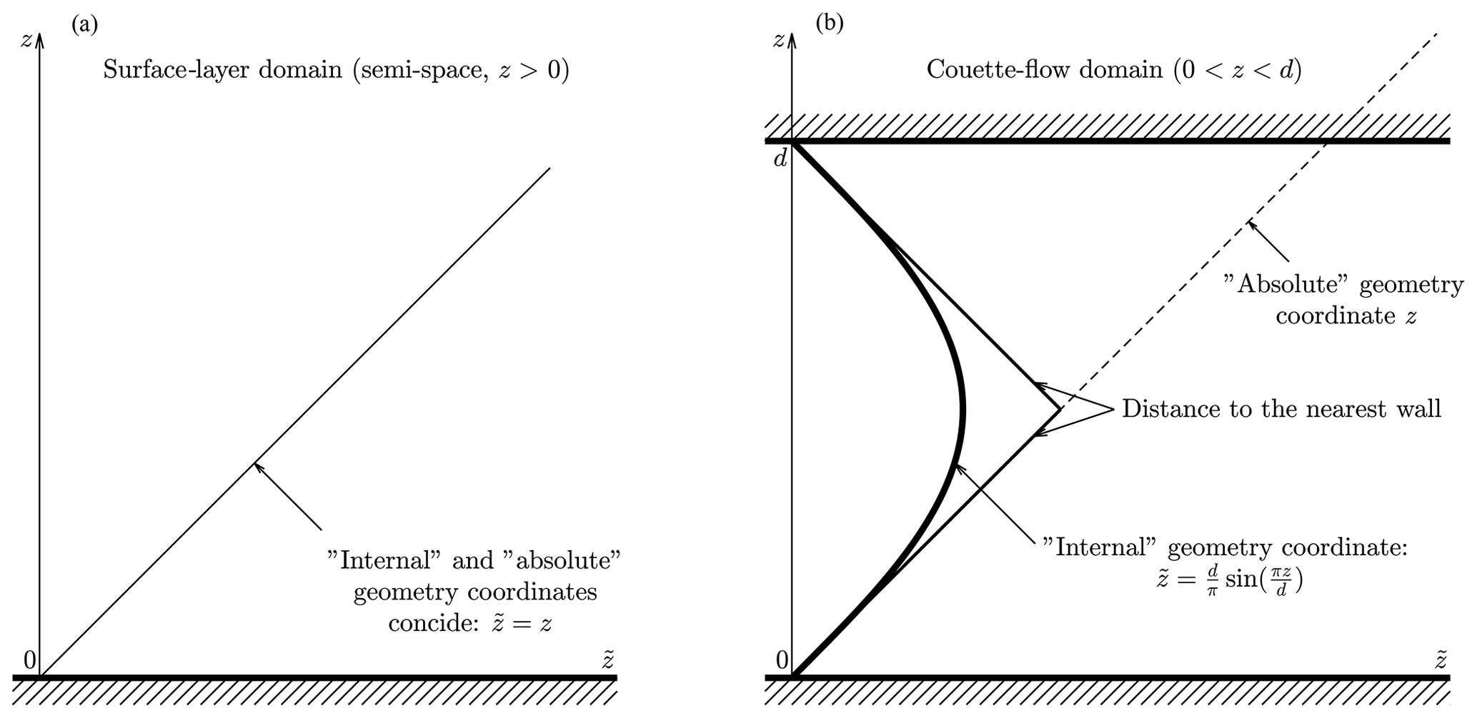
Figure 1Usual height, z, and vertical coordinate, , defined by Eq. (12) characterizing “absolute” and “internal” geometry of the domain, respectively. Panel (a) shows semi-space, z>0, where . Panel (b) shows the layer between two horizontal walls, , where coincides with the distance from nearest surface in its close vicinity, but essentially depends on the distances from both surfaces in the central part of the domain.
In our DNS total (turbulent + molecular) fluxes of momentum, τ, and potential temperature, Fz, are practically equal to the turbulent fluxes elsewhere beyond narrow near-wall sublayers where molecular transports dominate. In the Couette flow, the total fluxes are constant with height, exactly as in the surface-layer flows. Similarly, the flux-profile relations linking τ and Fz with vertical gradients of mean velocity, , and potential temperature, , as well as the budget equations for turbulent energies (in particular Eq. 6), are the same as in the surface-layer flows. The only difference is in the geometry of domains illustrated in Fig. 1.
Following Obukhov (1942), we distinguish between “absolute geometry” characterized by the usual height over the surface, z, and “internal geometry” characterized in Couette flow by specific vertical coordinate, , dictated by conformal mapping of the Couette-flow domain into the semi-space:
This coordinate reflects the influences of lower and upper walls on the fluid flow.
In semi-space, the “internal geometry” coincides with “absolute geometry”: . Thus, the vertical structure of the Couette flow in terms of coincides with the vertical structure of the surface-layer flow in terms of z. This allows for showing together the genuine dissipation rate calculated from DNS: , where ν is kinematic viscosity, and retrieved from atmospheric observations assuming the steady-state TKE budget.
In Figs. 2–4 we show our DNS data together with atmospheric data on the dissipation rate retrieved from observations in the surface layers indirectly:
-
via the Kolmogorov power law from measured spectra of TKE in the inertial subrange (Pearson et al., 2002), and
-
via the steady-state TKE budget Eq. (6) from the measured turbulent fluxes of momentum, τ, and potential temperature, Fz, and vertical gradient of mean wind velocity, .
In these figures DNS data are shown by bold coloured dots, and atmospheric data by light-grey symbols (Kadantsev et al., 2019).
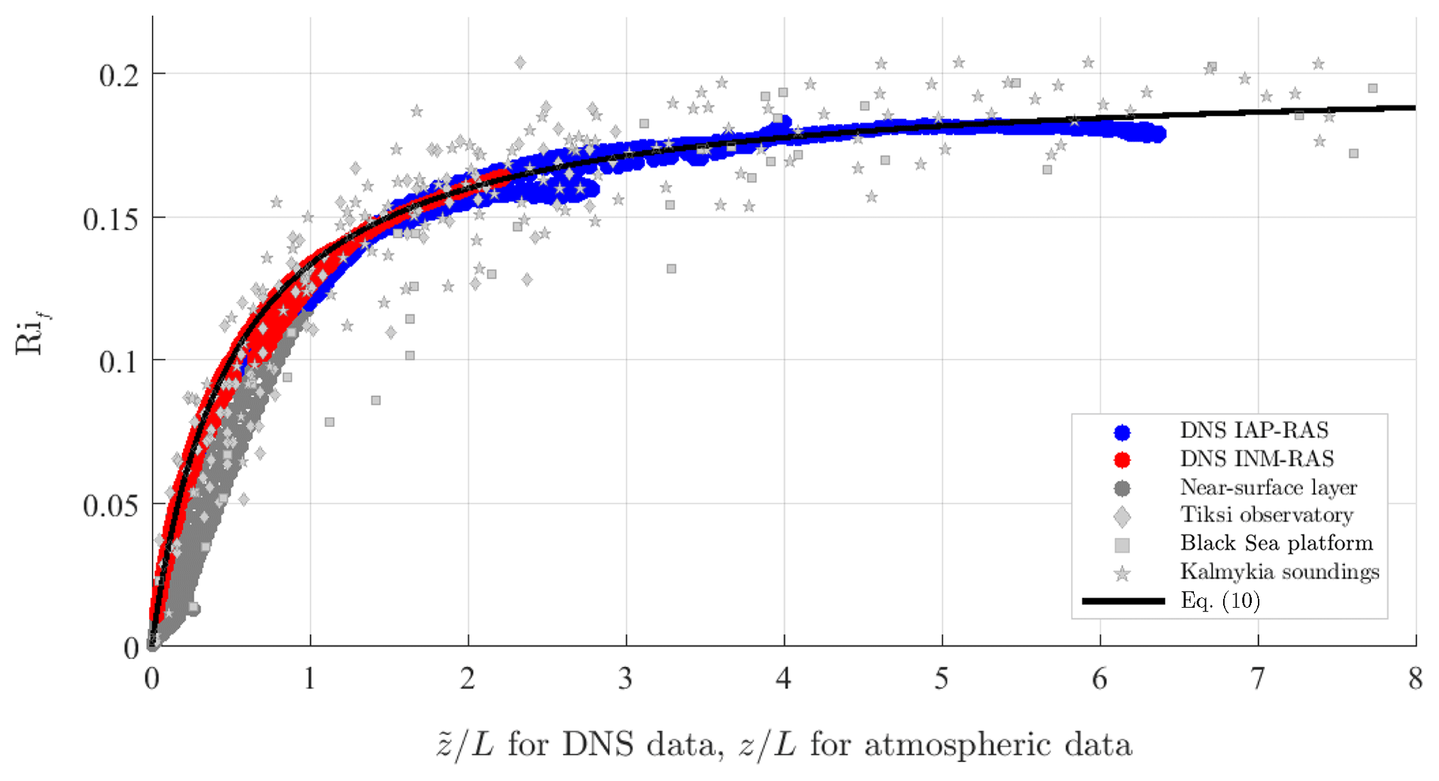
Figure 2Flux Richardson number, Rif, in stable stratification versus in Couette flow or versus z∕L in the atmospheric surface layer. Empirical data used for the calibration are obtained in two series of DNS runs employing INM-RAS code (red dots) and IAP-RAS code (blue dots). Atmospheric data are taken from Arctic coastal observatory Tiksi (light-grey diamonds), Black Sea offshore platform (light-grey squares), and acoustic soundings in Kalmykia steppe (light-grey stars). Dark-grey dots belong to the very narrow near-surface layer: . The solid black line shows Eq. (10) with the conventional value for the von Kármán constant, k=0.4, and new empirical value of R∞=0.2 just obtained from the best fit of Eq. (10) to DNS data from elsewhere beyond the layer , where molecular transports are significant and Eq. (10) is not necessarily relevant.
Figure 2 shows flux Richardson number, , versus dimensionless height, , in Couette flow; or versus z∕L in the atmospheric surface layer. The black curve is plotted after Eq. (10) taking the conventional value of the von Kármán constant, k=0.4, and our estimate of the maximal flux Richardson number, R∞=0.2, resulting from the best fit of Eq. (10) to DNS data. Notably, total (turbulent + molecular) fluxes of momentum, τ, and potential temperature, Fz, in Couette flow are constant across the flow which assures a very certain specification of Rif and L, and makes our DNS most suitable for calibrating the theory. We recall that Eqs. (10) and (11) are relevant to the well-developed turbulence regime where molecular transports are negligible, so that turbulent fluxes practically coincide with total fluxes. In our DNS this is true, except for the narrow transition layers dominated by molecular transport near the lower and upper walls: . Data from these layers are indicated by dark-grey points. The light-grey symbols show atmospheric data from the following sources: research observatory Tiksi in eastern Siberia near the Arctic Ocean coast (Grachev et al., 2018), offshore oceanographic platform in the Black Sea (Repina et al., 2009); and acoustic soundings over arid steppe in the Republic of Kalmykia in Southern Russia (Vazaeva et al., 2017). In spite of inevitable heterogeneity, non-stationarity, and other side effects, atmospheric data correlate quite well with DNS data.
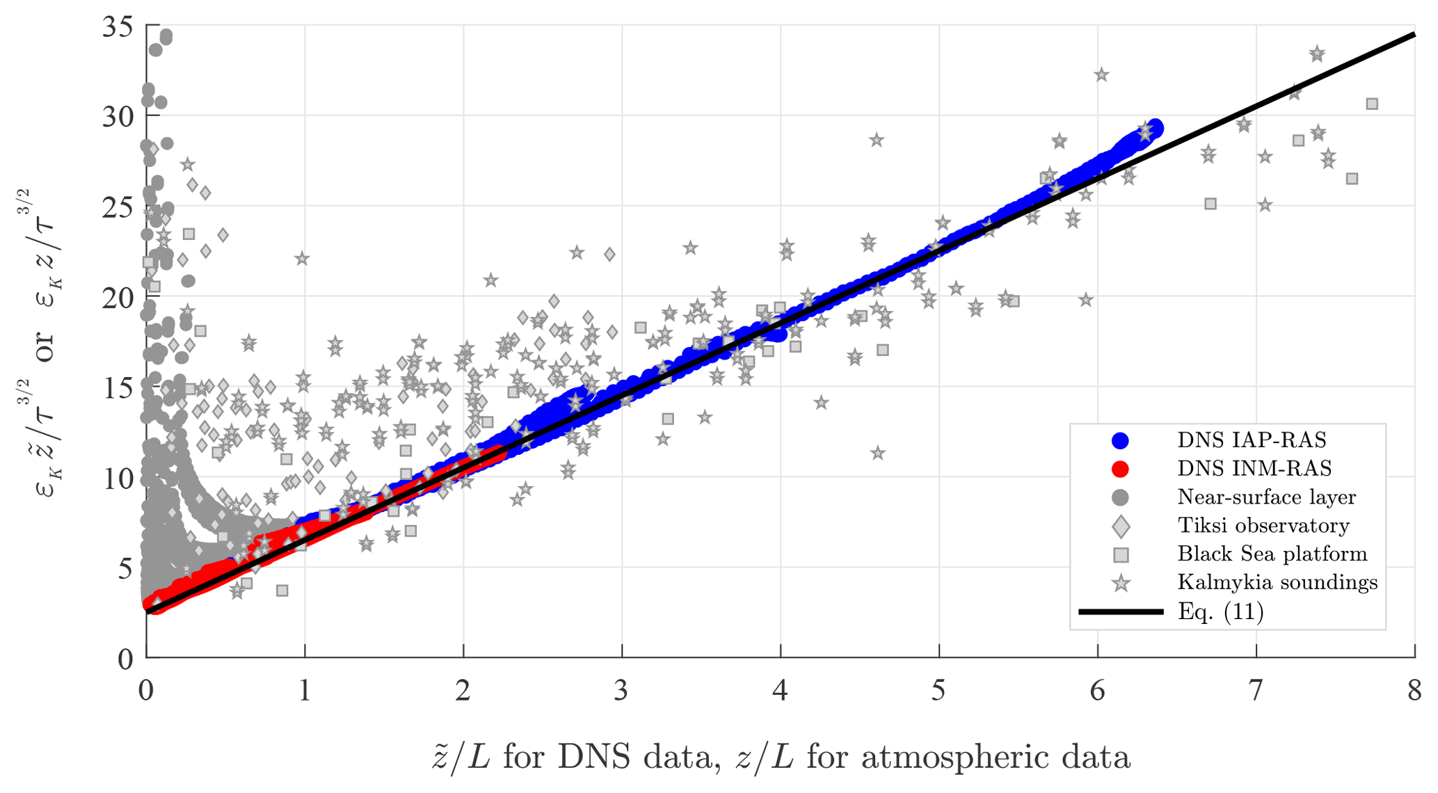
Figure 3Dimensionless dissipation rate in stable stratification, , versus in Couette flow or versus z∕L in the atmospheric surface layer. Empirical data are from the same sources as in Fig. 2. The solid black line shows Eq. (11) with k=0.4 and R∞=0.2. Dark-grey dots belong to the very narrow near-surface layer: , where molecular transports are significant and Eq. (11) is not relevant.
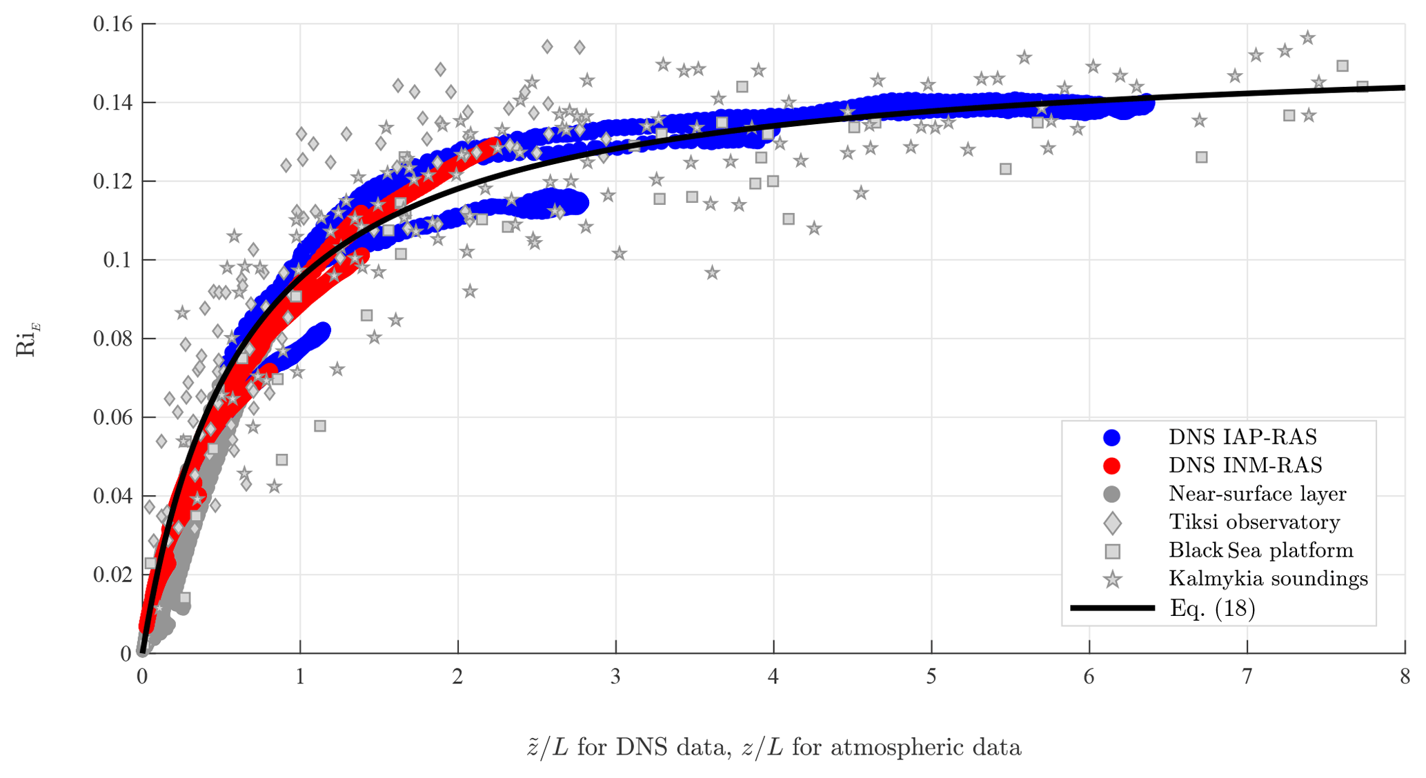
Figure 4The energy Richardson number, , versus in Couette flow or versus z∕L in the atmospheric surface layer. Empirical data are from the same sources as in Figs. 2 and 3. The solid black line shows Eq. (18) with k=0.4, R∞=0.2, and CP=0.62.
Figure 3 shows dimensionless dissipation rate, , versus z∕L after Eq. (11) and atmospheric data; and versus after DNS of Couette flow. All notations are the same as in Fig. 2. The theoretical curve plotted after Eq. (11) with k=0.4 and R∞=0.2 is fully consistent with experimental data, except for the narrow transition layer where Eq. (11) is irrelevant. Hence, Fig. 3 justifies the stability dependence of dissipation rate, Eq. (11), and provides additional confirmation to the empirical estimate of R∞=0.2.
In Fig. 2 we consider the flux Richardson number: , where turbulent fluxes (disregarding molecular contributions in the transition layer) appear in both the numerator and denominator. Hence uncertainties in both fluxes are somehow compensated. This is not the case in Fig. 3 showing vs. z∕L: the dissipation rate in the numerator is just total dissipation, whereas the momentum flux in the denominator disregards the molecular contribution. This causes the ugly looking but only natural dark-grey points on the left side of Fig. 3.
The concept of the TKE dissipation rate directly relates to the definition of the turbulent timescale, , and length scale, . Then Eq. (11) defines lT as a function of z∕L:
It has the asymptotic limits:
where the limits of EK∕τ in neutral stratification and in extremely stable stratification are just dimensionless constants. Our DNS yield the following estimates: and . The length scale similar to Eq. (13) was already revealed as inherent to spectra of turbulence in unstably stratified boundary-layer flows (Glazunov, 2014).
We emphasize that lT is the scalar characterizing turbulence as a whole. Contrastingly, turbulent mixing in different directions is characterized by the mixing-length vector with generally different streamwise (i=1), transverse (i=2), and vertical (i=3) components. We emphasize principal difference between the scalar length scale and vector mixing length. In literature, the words “turbulent length scale” and “turbulent mixing length” are often used as interchangeable. This causes intolerable confusion because different components of the mixing length differently depend on static stability (Zilitinkevich et al., 2013).
The above analyses are done for the simplest surface-layer (or Couette) flow, where dimensionless height z∕L (or plays the role of criterion quantifying the effect of stratification on turbulence. Luckily, our major result (Eqs. 11 and 13) can be easily extended to a wide range of stratified turbulent flows. We recall that stratified turbulence is characterized, besides EK, by turbulent potential energy (TPE), . Hence the effect of stratification on turbulence can be quantified by the “energy Richardson number” defined as
In contrast to traditional criteria, such as Ri (Eq. 4), Rif (Eq. 5), or z∕L, the energy Richardson number criterion is valid in heterogeneous and non-stationary flows, for any mechanisms of generation of turbulence (including breaking waves, oscillating grid, etc.) and in flows with complex geometry.
Expressing the dissipation rates of TKE and TPE in the steady state through the dissipation timescale, , the budget equations for TKE and TPE become
where CP is dimensionless parameter quantifying the difference between the dissipation rates of TKE and TPE (Zilitinkevich et al., 2013). Equations (16) and (17) in combination with Eq. (10) yield the following relations linking RiE with Rif or z∕L:
Figure 4 shows RiE versus z∕L or (like in previous figures) after our DNS and atmospheric observations. The theoretical curve is plotted after Eq. (18) taking k=0.4, R∞=0.2, and an empirical estimate of the dimensionless parameter CP=0.62 just obtained from the best fit of Eq. (18) to DNS data. Experimental data reveal the asymptotic limit:
Then, using Eq. (18) to express z∕L through RiE, Eq. (11) in terms of RiE becomes:
where εK(neutral) is dissipation rate in neutral stratification. In the surface layer ; but generally εK(neutral) depends on concrete energy-generation mechanisms and geometry of flow.
There is an essential advantage to RiE as criterion of stratification in numerical modelling. Turbulent fluxes are usually calculated through familiar diagnostic down-gradient formulations: and , where KM is eddy viscosity and KH is eddy conductivity. Then, finite-difference approximation of the gradients causes uncertainties in τ and Fz and, hence, in the Obukhov length, L (Eq. 3), flux Richardson number, Rif (Eq. 5), and gradient Richardson number, Ri (Eq. 4). Contrastingly, TKE and TPE are defined from prognostic budget equations accounting for turbulent diffusion which smooths the energies and assures quite a certain calculation of RiE.
The dissipation rate of TKE, εK, as dependent on static stability over years remained uncertain because of the impossibility of direct measurement of εK. Admittedly, εK can be retrieved via the TKE budget equation from the measured turbulent fluxes, τ and Fz, and mean-velocity gradient, , and also via the Kolmogorov power law from the measured spectra of TKE in the inertial subrange. However, these methods are only justified in stationary and horizontally homogeneous flows and require fully controlled conditions. These provisions, practically unachievable in atmospheric experiments, make estimates of εK from atmospheric observations rather uncertain. The wide spread of atmospheric data is clearly seen in our figures. Moreover, available atmospheric data cover only weakly to moderately stable stratifications typical of the surface layer. To avoid these difficulties, we performed topical DNS of the steady-state stably stratified turbulent Couette flows up to the strongest attainable stratifications, combined direct data from DNS with data retrieved from atmospheric observations, and employed theoretical analysis to reveal asymptotic behaviour of the mean velocity gradient and the dissipation rate in extremely stable stratification, namely as where L is the Obukhov length scale.
By providential coincidence, the formulations happen to be precisely the same in the asymptotic limit and in the weakly stable stratifications typical of atmospheric surface layer. This yields simple analytical formulations of the dimensionless velocity gradient, , and dissipation rate, , as universal functions of z∕L (Eqs. 9 and 11) across the whole range of stratifications from neutral to extremely stable.
Universal analytical formulation of versus z∕L yields the single-valued relations linking z∕L as the criterion of stratification in the surface-layer flow or as the same criterion in Couette flow with alternative criterions: flux Richardson number, Rif (Eq. 5), and the newly introduced “energy Richardson number”, RiE (Eq. 13), applicable to any turbulent regimes. This opens up prospects for extending the obtained dependence of dissipation rate on static stability to any stably stratified turbulent flows.
The data can be accessed at https://doi.org/10.23728/b2share.fd1f300ec18b4fe1bd3d811630b0 (Kadantsev et al., 2019).
SZ conceived the concept, did theoretical derivations, and led the research. EM (author of INM-RAS DNS code) and OD (author of IAP-RAS DNS code) carried out independent numerical simulation of turbulent Couette flow aiming at verification and validation of the theory. IR collected and analysed complementary data from observations in the atmospheric surface layer over various types of the Earth surface. EK utilized all these data, carried out the entire work on verification and validation, and produced all figures. YT and AG contributed to theoretical analyses. All authors participated in writing the manuscript.
The authors declare that they have no conflict of interest.
This article is part of the special issue “Pan-Eurasian Experiment (PEEX)”. It is not associated with a conference.
The authors acknowledge support from the Academy of Finland project ClimEco no. 314
798/799; Russian Foundation for Basic Research (project nos. 18-05-60299, 16-05-01094 A,
18-55-11005). Analysis of data from atmospheric observation was supported from the
Russian Science Foundation grant no. 17-17-01210. Post-processing of numerical data from
IAP was supported by the Russian Science Foundation grant no. 15-17-20009 and Russian
Foundation for Basic Research grants nos. 17-05-00703 and 18-05-00292.
Edited by: Imre Salma
Reviewed by: three anonymous
referees
Druzhinin, O. A., Troitskaya, Y. I., and Zilitinkevich, S. S.: Stably stratified airflow over a waved water surface. Part 1: Stationary turbulence regime, Q. J. Roy. Meteor. Soc., 142, 759–772, https://doi.org/10.1002/qj.2677, 2016.
Garratt, J. R.: The atmospheric boundary layer, Cambridge University Press, UK, 316 pp. 1992.
Glazunov, A. V.: Numerical simulation of stably stratified turbulent flows over an urban surface: Spectra and scales and parameterization of temperature and wind-velocity profiles, Izv. Atmos. Ocean. Phy., 50, 356–368, https://doi.org/10.1134/S0001433814040148, 2014.
Grachev, A. A., Persson, P. O. G., Uttal, T., Akish, E. A., Cox, C. J., Morris, S. M., Fairall, C. W., Stone, R. S., Lesins, G., Makshtas, A. P., and Repina, I. A.: Seasonal and latitudinal variations of surface fluxes at two Arctic terrestrial sites, Clim. Dynam., 51, 1793–1818, https://doi.org/10.1007/s00382-017-3983-4, 2018.
Kadantsev, E., Mortikov, E., Druzhinin, O., and Repina, I.: Dissipation rate of turbulent kinetic energy: direct numerical simulation and atmospheric data, https://doi.org/10.23728/b2share.fd1f300ec18b4fe1bd3d811630, 2019.
Katul, G., Porporato, A., Shah, S., and Bou-Zeid, E.,: Two phenomenological constants explain similarity laws in stably stratified turbulence, Phys. Rev. E, 89, 023007, https://doi.org/10.1103/PhysRevE.89.023007, 2014.
Kolmogorov, A. N.: Equations of turbulent motion for an incompressible fluid, Izv. An. SSSR Fiz. 6, 56–58, 1942.
Monin, A. S. and Obukhov, A. M.: Basic laws of turbulent mixing in the atmospheric surface layer, Trudy Geofiz. Inst. Akad. Nauk SSSR, 24, 163–187, 1954.
Monin, A. S. and Yaglom, A. M.: Statistical Fluid Mechanics, Volume 1, MIT Press, Cambridge, Massachusetts, 769 pp., 1971.
Mortikov, E. V.: Numerical simulation of the motion of an ice keel in a stratified flow, Izv. Atmos. Ocean. Phy., 52, 108–155, https://doi.org/10.1134/S0001433816010072, 2016.
Mortikov E. V., Glazunov A. V., and Lykosov V. N.: Numerical study of plane Couette flow: turbulence statistics and the structure of pressure-strain correlations, Russ. J. Numer. Anal. M., 34, in press, 2019.
Obukhov, A. M.: Ueber die Verteilung des Turbulenzmaßstabes in Strömen mit beliebigen Querschnitt, J. Appl. Math. Mech., 4, 209–220, 1942.
Obukhov, A. M.: Turbulence in thermally inhomogeneous atmosphere, Turbulence in thermally inhomogeneous atmosphere, Trudy Inst. Teor. Geofiz. Akad. Nauk SSSR, 1, 95–115, 1946 (translated in Boundary-Layer Meteor, 3, 7–29, 1971).
Pearson, B., Krogstad, P. Å., and Van De Water, W.: Measurements of the turbulent energy dissipation rate, Phys. Fluids, 14, 1288–1290, https://doi.org/10.1063/1.1445422, 2002.
Repina, I. A., Chukharev, A. M., Goryachkin, Y. N., Komarova, N. Y., and Pospelov, M. N.: Evolution of air-sea interaction parameters during the temperature front passage: The measurements on an oceanographic platform, Atmos. Res., 94, 74–80, https://doi.org/10.1016/j.atmosres.2008.11.007, 2009.
Stull, R.: An Introduction to Boundary Layer Meteorology, Kluwer Acad. Press, Dordrecht, Netherlands, 670 pp. 1997.
Vazaeva, N. V., Chkhetiani, O. G., Kouznetsov, R. D., Kallistratova, M. A., Kramar, V. F., Lyulyukin, V. S., and Kuznetsov, D. D.: Estimating helicity in the atmospheric boundary layer from acoustic sounding data, Izv. Atmos. Ocean. Phy., 53, 174–186, https://doi.org/10.1134/S0001433817020104, 2017.
Zilitinkevich, S. S., Elperin, T., Kleeorin, N., Rogachevskii, I., and Esau, I. N.: A hierarchy of energy- and flux-budget (EFB) turbulence closure models for stably stratified geophysical flows, Bound.-Lay. Meteorol., 146, 341–373, https://doi.org/10.1007/s10546-012-9768-8, 2013.