the Creative Commons Attribution 4.0 License.
the Creative Commons Attribution 4.0 License.
 | 19 Feb 2019
Surface erythemal UV irradiance in the continental United States derived from ground-based and OMI observations: quality assessment, trend analysis and sampling issues
Lorena Castro García
Jing Zeng
Connor Dennhardt
Nickolay A. Krotkov
Surface full-sky erythemal dose rate (EDR) from the Ozone Monitoring Instrument (OMI) at both satellite overpass time and local noon time is evaluated against ground measurements at 31 sites from the US Department of Agriculture's (USDA) UV-B Monitoring and Research Program (UVMRP) over the period of 2005–2017. We find that both OMI overpass and solar noon time EDR are highly correlated with the measured counterparts (with a linear correlation coefficient of 0.90 and 0.88, respectively). Although the comparison statistics are improved with a longer time window (0.5–1.0 h) for pairing surface and OMI measurements, both OMI overpass and local noon time EDRs have 7 % overestimation that is larger than 6 % uncertainty in the ground measurements and show different levels of dependence on solar zenith angle (SZA) and to lesser extent on cloud optical depth. The ratio of EDR between local noon and OMI overpass time is often (95 % in frequency) larger than 1 with a mean of 1.18 in the OMI product; in contrast, the same ratio from surface observation is normally distributed with 22 % of the times less than 1 and a mean of 1.38. This contrast in part reflects the deficiency in the OMI surface UV algorithm that assumes constant atmospheric conditions between overpass and noon time. The probability density functions (PDFs) for both OMI and ground measurements of noontime EDR are in statistically significant agreement, showing dual peaks at ∼20 and ∼200 mW m−2, respectively; the latter is lower than 220 mW m−2, the value at which the PDF of daily EDR from ground measurements peaks, and this difference indicates that the largest EDR value for a given day may not often occur at local noon. Lastly, statistically significant positive trends of EDR are found in the northeastern US in OMI data, but opposite trends are found within ground-based data (regardless of sampling for either noontime or daily averages). While positive trends are consistently found between OMI and surface data for EDR over the southern Great Plains (Texas and Oklahoma), their values are within the uncertainty of ground measurements. Overall, no scientifically sound trends can be found among OMI data for aerosol total and absorbing optical depth, cloud optical depth and total ozone to explain coherently the surface UV trends revealed either by OMI or ground-based estimates; these data also cannot reconcile trend differences between the two estimates (of EDR from OMI and surface observations). Future geostationary satellites with better spatiotemporal resolution data should help overcome spatiotemporal sampling issues inherent in OMI data products and therefore improve the estimates of surface UV flux and EDR from space.
- Article
(7667 KB) - Full-text XML
-
Supplement
(994 KB) - BibTeX
- EndNote


The amount of surface solar UV radiation (200–400 nm) reaching the earth's surface has substantial impacts on human health and ecosystems (Andrady et al., 2015; WMO, 2014). For example, about 90 % of nonmelanoma skin cancers are associated with exposure to solar UV radiation in the US (Koh et al., 1996). Bornman and Teramura (1993) and Caldwell et al. (1995) showed the negative effects of UV radiation on plant growth and tissues. Since the discovery of the significant ozone depletion in the Antarctic region (Farman et al., 1985) and midlatitudes (Fioletov et al., 2002), subsequent effects on surface UV levels have received attention. As a result, great efforts have been made to monitor surface UV radiation from both satellite and ground instruments in the past few decades (Bigelow et al., 1998; Sabburg et al., 2002; Levelt et al., 2006; Buntoung and Webb, 2010; Lakkala et al., 2014; Pandey et al., 2016; Krzyścin et al., 2011; Utrillas et al., 2013). Although satellite measurements provide a better spatial coverage of the surface UV radiation, they (similar to ground-based observations) are not only affected by instrument errors (Bernhard and Seckmeyer, 1999), but are also subject to uncertainties in the algorithms used to derive surface UV radiation. Therefore, evaluation of satellite-based estimates of surface UV radiation against available ground measurements at many locations around the world is needed to characterize the errors toward further refinement of the surface UV estimates.
The solar spectral irradiance (in mW m−2 nm−1) is usually measured by ground and satellite instruments. In addition, the erythemally weighted irradiance has been widely used to describe the sunburning or reddening effects (McKenzie et al., 2004). Erythemally weighted irradiance or erythemal dose rate (EDR; in mW m−2) is defined as the solar irradiance on a horizontal surface weighted with the erythemal action spectrum (McKinlay and Diffey, 1987); it can be further divided by 25 mW m−2 to derive the UV index – an indicator of the potential for skin damage (WMO, 2002). Hence, the UV index is commonly used as a UV exposure measure for the general public and in epidemiological studies in many parts of the world (Eide and Weinstock, 2005; Lemus-Deschamps and Makin, 2012; Walls et al., 2013). In the US, several ground UV monitoring networks that respond to changes in the surface UV radiation have been established (Bigelow et al., 1998; Sabburg et al., 2002; Scotto et al., 1988). Currently, the UV-B Monitoring and Research Program (UVMRP) initiated by the US Department of Agriculture (USDA) and the NEUBrew (NOAA-EPA Brewer Spectrophotometer UV and Ozone Network) remain as the two active operating networks providing surface UV data in the US.
The goal of this study is to use UVMRP datasets to evaluate the Ozone Monitoring Instrument (OMI)-based estimates of the surface UV radiation in the past decade in the US. As a successor to the Total Ozone Mapping Spectrometer (TOMS), whose surface UV data (such as erythemally weighted irradiance) have been extensively evaluated in the past (Arola et al., 2005; Cede et al., 2004; Kalliskota et al., 2000; Kazantzidis et al., 2006; McKenzie et al., 2001), OMI data have a finer spatial and spectral resolution and thereby bear more advanced capability for characterizing the spatial distribution of the surface UV radiation. TOMS data records span from 1978 to 2005, and many past studies have shown that TOMS surface UV data overestimated the ground observational data at many sites. OMI was launched into space in July 2004 as part of the Aura satellite (Levelt et al., 2006), and it has started to collect data from August 2004 to the present. While there have been a number of studies evaluating the OMI surface UV data with ground observations, these studies, as shown in Table 1, have mainly focused on Europe (Antón et al., 2010; Buchard et al., 2008; Ialongo et al., 2008; Kazadzis et al., 2009a; Tanskanen et al., 2007; Weihs et al., 2008; Zempila et al., 2016), South America (Cabrera et al., 2012), high latitudes (Bernhard et al., 2015) and the tropics (Janjai et al., 2014). These studies evaluated OMI spectral irradiance, EDR and erythemally weighted daily dose (EDD) within different time periods. Most comparisons show positive bias up to 69 %, with few showing negative bias up to −10 %.
This study differs from the past studies in the following ways. Firstly, we conducted a comprehensive evaluation of the OMI surface UV data from 2005 to 2017 covering the continental US. The evaluation was made for erythemally weighted irradiance at both local solar noon and satellite overpass times, and the evaluation statistics not only concern mean bias (MB) but also the probability density function (PDF), cumulative distribution function (CDF) and variability of the UV data. Secondly, a trend analysis of the surface UV irradiance from both ground observation and OMI was performed, with a special focus on the effects of the temporal sampling. The analysis addresses whether the once-per-day sampling from the polar-orbiting satellite would have any inherent limitation for the trend analysis of surface UV data. Finally, the error characteristics in the OMI surface UV data were examined to understand the underlying sources (such as from treatment of clouds and assumption of constant atmospheric conditions between the local solar noon and satellite overpass time). The investigation yields recommendations for future refinement of the OMI surface UV algorithm.
The paper is organized as follows: Sect. 2 describes the satellite and ground observational data, the methodology is discussed in Sect. 3, Sect. 4 presents the results and Sect. 5 summarizes the findings.
Table 1Summary of previous studies evaluating OMI surface UV data against ground observation. Most of the comparisons shown here are for all-sky conditions unless noted otherwise.
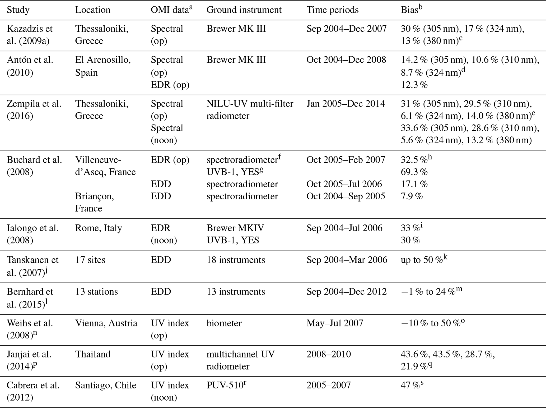
aSpectral represents the OMI spectral irradiance data, EDR is the erythemal dose rate and EDD is the erythemally weighted daily dose. Op corresponds to the OMI data at its overpass time while noon means the data at local solar noon time. b The validation statistic shown here is the bias with each study using slightly different ways of calculation. c The bias here is calculated as the median (OMI/Ground − 1)×100. d The bias is calculated as , where N is the total number of data points. e The bias is calculated as the mean (OMI − Ground)/Ground × 100. f The spectroradiometer used here is thermally regulated Jobin Yvon H10 double monochromator. g The broadband UVB-1 is from Yankee Environmental System (YES). h The bias is calculated as , where N is the total number of data points. i Same as h. j This study evaluated OMI surface EDD at 17 ground sites representing different latitudes, elevations and climate conditions with 18 instruments, which include single and double Brewer spectrophotometers, NIWA UV spectrometer systems, a DILOR XY50 spectrometer and SUV spectroradiometers. k The bias is calculated as in c. For sites significantly affected by absorbing aerosols or trace gases, the bias can be up to 50 %. l This study evaluated OMI EDD at 13 ground stations located throughout the Arctic and Scandinavia from 60 to 83∘ N. The instruments installed include a single-monochromator Brewer spectrophotometer and GUV-541 and GUV-511 multi-filter radiometers from Biospherical Instrument Inc. (BSI). m Same as c. n This study evaluated OMI UV index at 6 ground stations in the city of Vienna, Austria, and its surroundings. Six biometers (Model 501, Solar Light Company, Inc.) were used. o The bias is calculated as (OMI/Ground − 1)×100 and the result for clear-sky conditions is shown here. p This study evaluated OMI UV index at four tropical sites in Thailand with each site having different time periods of data between 2008 and 2010. The ground instrument installed is a multichannel UV radiometer (GUV-2511) manufactured by BSI. q The bias is calculated as h, representing the four sites, respectively. r PUV-510 is a multichannel filter UV radiometer centered at 305, 320, 340 and 380 nm. sThe bias is calculated as (OMI − Ground)/OMI × 100.
2.1 OMI data
OMI aboard the NASA Aura spacecraft is a nadir-viewing spectrometer (Levelt et al., 2006) that measures solar reflected and backscattered radiances in the range of 270 to 500 nm with a spectral resolution of about 0.5 nm. The 2600 km wide viewing swath and the sun-synchronous orbit of Aura provides a daily global coverage, with an equatorial crossing time at ∼13:45 LT (local time). The spatial resolution varies from 13×24 km2 (along × cross) at nadir to 50×50 km2 near the edge. OMI retrieves total column ozone, total column amount of trace gases, SO2, NO2, HOCO, aerosol characteristic and surface UV (Levelt et al., 2006).
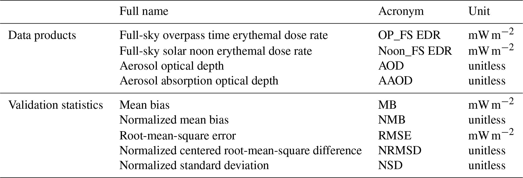
Table 2OMI data products and validation statistics used in the current study.
The OMI surface UV algorithm has its heritage from the TOMS UV algorithm developed at the NASA Goddard Space Flight Center (GSFC) (Eck et al., 1995; Herman et al., 1999; Krotkov et al., 1998, 2001, 2002; Tanskanen et al., 2006). In the first part of the algorithm, the surface-level UV irradiance at each OMI pixel under clear-sky conditions is estimated from a lookup table that is computed from a radiative transfer model for different values of total column ozone, surface albedo and solar zenith angle (SZA). The lookup table was called twice, once to calculate the surface UV irradiance at the satellite overpass time and once at the local solar noon. The only difference between these two lookup tables is the SZAs, with one representing the SZAs at the overpass time and the other representing the solar noon, while the total column ozone and cloud optical thickness (COT) are assumed to stay constant. The second step is to correct the clear-sky surface UV irradiance for a given OMI pixel due to the effects of cloud and nonabsorbing aerosols. The cloud-correction factor is derived from the ratio of measured backscatter irradiances and solar irradiances at 360 nm along with OMI total column ozone amount, surface monthly minimum Lambertian effective reflectivity (LER) and surface pressure. The effects of absorbing aerosols are also adjusted in the current surface UV algorithm based on a monthly aerosol climatology as described in Arola et al. (2009).
The second step of the cloud correction mentioned above follows radiative transfer calculations that assume a homogeneous, plane-parallel water-cloud model with Rayleigh scattering and ozone absorption in the atmosphere (Krotkov et al., 2001). The COT is assumed to be spectrally independent and the cloud-phase function follows the C1-cloud model (Deirmendjian, 1969). This cloud model is also used to calculate the angular distribution of 360 nm radiance at the top of the atmosphere, which is used to derive an effective COT. The effective COT is the same as the actual COT for a homogeneous cloud plane-parallel model. The effective COT is saved to a lookup table to use for cloud correction.
OMI surface UV data products (or OMUVB in shorthand) include (a) spectral irradiance (mW m−2 nm−1) at 305, 310, 324 and 380 nm at both the local solar noon and OMI overpass time; (b) erythemal dose rate (mW m−2) at both the local solar noon and OMI overpass time; and (c) erythemally weighted daily dose (J m−2). The spectral irradiances assume a triangular slit function with full width at half maximum of 0.55 nm. The EDD is computed by applying the trapezoidal integration method to the hourly EDR with the assumption that the total column ozone and COT remain the same throughout the day. In addition, the OMUVB products include information on data quality related to row anomaly, SZA and COT, which are used in the present study. We also use the aerosol products from the OMAERUV algorithm (Torres et al., 2007). The OMI OMAERUV algorithm uses two wavelengths in the UV region (354 and 388 nm) to derive aerosol extinction and absorption optical depth. The aerosol products (OMAERUV) retrieve aerosol optical depth (AOD), aerosol absorption optical depth (AAOD) and single scattering albedo at 354, 388 and 500 nm.
In the current study, both OMI level 2 (v003) and level 3 (v003) products are used. The level 2 products provide swath-level data products while level 3 products are gridded daily products on a 1∘ × 1∘ horizontal grid. Two variables from OMUVB level 2 products (Table 2) are used: (1) full-sky solar noon erythemal dose rate denoted as Noon_FS EDR and (2) full-sky overpass time erythemal dose rate denoted as OP_FS EDR. In addition, full-sky solar noon EDR from the OMUVBd (“d” denotes daily) level 3 products and AOD and AAOD from OMAERUVd level 3 products are used. These level 3 datasets are mainly used for conducting trend analysis in Sect. 4.4 unless noted otherwise, while the rest of the data analysis uses the level 2 datasets. All the datasets are from January 2005 to December 2017 and row anomaly is checked during data analysis for level 2 datasets.
2.2 Ground observation data
Currently, the UVMRP operates 36 climatological sites for long-term monitoring of surface UV radiation around different ecosystem regions (https://uvb.nrel.colostate.edu/UVB/uvb-network.jsf, last access: 21 January 2019). Of the 36 climatological sites, five are located in New Zealand, South Korea, Hawaii, Alaska and Canada, while 31 sites are in the continental US, with the majority of them located in agricultural or rural areas and a few in urban areas. Among these 31 sites, one site started operation after 2014 and one after 2006, and all other sites started earlier than 2006. In the current study, we use the one site in Canada and 30 of the 31 sites in the continental US and we exclude one site where operation started after 2014 (Fig. 1).
All sites measure global irradiance using a UVB-1 pyranometer manufactured by Yankee Environmental Systems (YES). Since 1997, these broadband radiometers have been calibrated and characterized annually at the Central UV Calibration Facility (CUCF), located in Boulder, and have then been cycled through Mauna Loa Observatory (MLO), Hawaii, for calibration after around 2009. The annual characterization process includes laboratory tests for spectral and cosine response change in the radiometer. For the calibration, the UVMRP broadband radiometer is collocated with three of CUCF's YES UVB-1 standard radiometers (the triad) and a precision spectroradiometer in the field for 2 weeks. The absolute calibration factor of each UVMRP radiometer is determined by comparing its voltage output to the standard triad, which is in turn frequently calibrated against the collocated spectroradiometer. Because the spectral response functions of the UVMRP broadband radiometer do not precisely match the erythemal action spectrum (McKinlay and Diffey, 1987), corrections that depend on SZA and total column ozone are needed. More detailed calibration and characterization procedures are described in Lantz et al. (1999). The erythemal UV irradiance used in the current work is prepared with SZA-dependent calibration factors that assume total column ozone is 300 DU (Gao et al., 2010). Past studies have shown that the UVMRP broadband radiometer differs from the triad by 0.1 %–2.8 % for SZA ranging from 20 to 80∘ (Seckmeyer et al., 2005; McKenzie et al., 2006). The calibration from the spectroradiometer to the standard triad results in an uncertainty of approximately ±5 % and the overall uncertainty for the UVMRP broadband radiometers has been estimated at approximately ±6 % (Kimlin et al., 2005). The YES UVB-1 instrument takes measurement every 15 s, which are aggregated into 3 min averages.
In this work, we use the 3 min averaged erythemally weighted irradiance at 31 sites in the continental US and information for each site is described in Table S1 in the Supplement. Except for site TX41, for which data are available since August 2006, we use data from January 2005 to December 2017 for the rest of the sites.
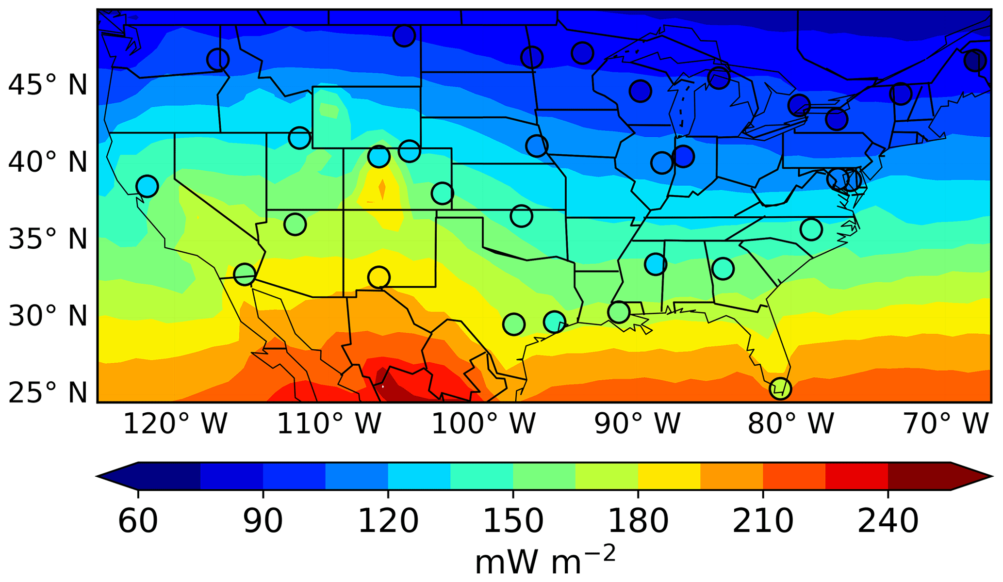
Figure 1Map of OMI level 3 EDR (mW m−2) at solar noon time under full-sky conditions averaged over 2005–2017, overlaid with 31 ground observational sites averaged over 2005–2017 around solar noon time with min.
3.1 Spatial collocation and temporal averaging of data
Since OMI data represent an average over a ground pixel ( km2 for nadir viewing and km2 for off-nadir viewing) and ground measurements are point measurements that cover a small area, previous work in Table 1, studies of Kazadzis et al. (2009b) and Zempila et al. (2018), and studies using TOMS data have investigated the effects of the selection of a collocation distance between the center of an OMI ground pixel and the ground observational site and/or the averaging time period around OMI overpass time and local solar noon on the evaluation results. For example, Weihs et al. (2008) found that the variability, defined as the absolute sum of the difference between the average mean bias between OMI- and ground-measured UV index at any station and the average mean bias from all stations divided by the total number of measurements, increases with increasing collocation distance but decreases with increasing averaging time period. Zempila et al. (2016) compared OMI spectral irradiances at 305, 310, 324 and 380 nm with ground observations considering spatial collocation and temporal averaging windows. It was shown that the choice of collocation distance (10, 25 or 50 km) plays a negligible role in the comparison in terms of the correlation coefficient and mean bias. However, the selection of a longer averaging time period (from ±1 to ±30 min) results in a significant improvement under full-sky conditions for both OMI overpass and solar noon time comparison. Chubarova et al. (2002) evaluated the difference between TOMS overpass surface UV and ground data taken over different time windows around TOMS overpass time. The results showed that the calculated correlation coefficient of these two datasets nonlinearly increases with the increasing averaging windows (from ±1 to ±60 min) and stays nearly constant from ±60 to ±90 min.
In this work, we will examine the separate effects of spatial collocation and temporal averaging on evaluation results. Firstly, for each ground site, its observation is paired with the OMI data at the pixel level if the center of that pixel is within the distance (D) of 50 km from that ground site. Then the ground observational data at each site are taken within (ΔT of) ±5 min around the OMI overpass time or the local solar noon time at that pixel. Correspondingly, there will be two to three ground data found, the temporal mean of which will be paired up with the OMI data from that pixel for subsequent comparison. Further evaluation is conducted by changing different D values to 10 and 25 km and/or ΔT values of ±10, ±30 and ±60 min around OMI overpass time and local solar noon time. Consequently, a total of 12 sets of paired data are generated for the evaluation, as a result of a different combination of three D values and four ΔT values used for spatially and temporally collocating OMI and ground data. For a given ΔT, there are ∼100 000, ∼67 000 and ∼17 000 data pairs at all of the ground sites for D values of 50, 25 and 10 km, respectively.
3.2 Validation statistics
First, we present several commonly used validation statistics (Table 2): mean bias (MB) calculated in Eq. (1), normalized mean bias (NMB) in Eq. (2), the root-mean-square error (RMSE) in Eq. (3) and correlation coefficient (R). We also show the overall evaluation of OMI surface UV data against ground observation in the form of a Taylor diagram (Taylor, 2001) (see Fig. 3a). A Taylor diagram provides a statistic summary of OMI data evaluated against ground observation in terms of correlation coefficient R (the cosine of polar angles); the ratio of standard deviations between OMI and ground observational data (the normalized standard deviation – NSD) shown in the x and y axis, respectively; and the normalized centered root-mean-square difference (NRMSD) in Eq. (4), shown as the radius from the expected point, which is located at the point where R and NSD are unity.
where i is the ith paired (OMI–ground) data point, N is the total number of paired data points, and EDR(OMI,i) and EDR(Ground,i) are the ith EDR from OMI and ground observation, respectively. and are the mean of N number of OMI and ground data, respectively. Both correlation coefficients in the Taylor diagram and the scatter plot are obtained from the ordinary linear least squares method.
To determine whether the calculated MB or NMB are statistically significant, a t test for differences of mean under serial dependence is applied (Wilks, 2011). This two-sample t test assumes a first-order autoregression in the data. The computed two-tailed p value of less than 0.025 indicates that the difference between the means for the paired data (OMI and ground EDR) would be statistically significant at the 95 % confidence level. In addition, we calculate the PDF and CDF of OMI and ground observational data. A Kolmogorov–Smirnov (K–S) test (Wilks, 2011) is performed to compare the CDFs of the OMI and ground datasets. The K–S test is represented by the following formula:
If D is greater than the critical value, 0.84 (m is the total number of data points), then the null hypothesis that the two datasets were drawn from the same distribution will be rejected at the 99 % confidence level.
3.3 Trend analysis
Following the work of Weatherhead et al. (1997, 1998), the trend of surface UV irradiance from OMI and ground observation can be estimated using the following linear model:
where T is the total number of months considered and t is the month index, starting from January 2005 to December 2017. Yt is the monthly mean surface UV irradiance either from OMI or the ground observation in the US and C is a constant. represents the linear trend function and ω is the magnitude of the trend per year. St is a seasonal component, represented in the following form:
Nt is the noise not represented by the linear model and is often assumed to be a first-order autoregressive model, which can be expressed as
where Nt−1 is the noise from month (t−1); ϕ is the autocorrelation between Nt and Nt−1; and εt is the white noise which should be approximately independent, normally distributed with zero mean and common variance .
As described in Weatherhead et al. (1998), generalized least squares (GLS) regression was applied to Eq. (6) to derive the approximation of ω and its standard deviation σω as
where is the number of years of the data used in the analysis and σN is the standard deviation of Nt. We will consider the trend significant at the 95 % confidence level if . Such linear models have been widely used to study the various environmental monthly time series data in the previous studies (Boys et al., 2014; Zhang and Reid, 2010; Weatherhead et al., 2000).

Figure 2Scatter plots of OMI EDR data with ground observations from year 2005 to 2017. (a, b) show the comparisons of OMI OP_FS and Noon_FS EDR with measurements at all of the 31 ground observational sites, respectively, while (c, d) only show the comparisons of OMI EDR with ground measurements at Homestead, Florida (FL01). In each scatter plot, also shown is the correlation coefficient (R), the root-mean-square error (RMSE), the number of collocated data points (N), the density of points (the color bar), the best-fit linear regression line (the dashed black line) and the 1:1 line (the solid black line).
4.1 Spatial and temporal inter-comparison
Figure 1 shows the map of OMI level 3 EDR at solar noon time under full-sky conditions averaged from 2005 to 2017, overlaid with 31 ground observational sites of EDR averaged from the same local noon time. First, we find that OMI data show a meridional gradient with the dose rate increasing from ∼80 mW m−2 in the northern US to ∼203 mW m−2 in the southern US. At higher-elevation regions such as in Colorado, OMI-derived EDRs are larger than other areas of the same latitude zone. In comparison, the ground sites range from ∼73 mW m−2 in the northern US to a maximum of ∼190 mW m−2 for site NM01 in the southern US, generally capturing the OMI meridional gradient well. At most sites, OMI data overestimate the ground observation by more than 5 %, with sites in Steamboat Springs, Colorado (CO11); Burlington, Vermont (VT01); and Homestead, Florida (FL01), showing the highest bias of more than 15 %.
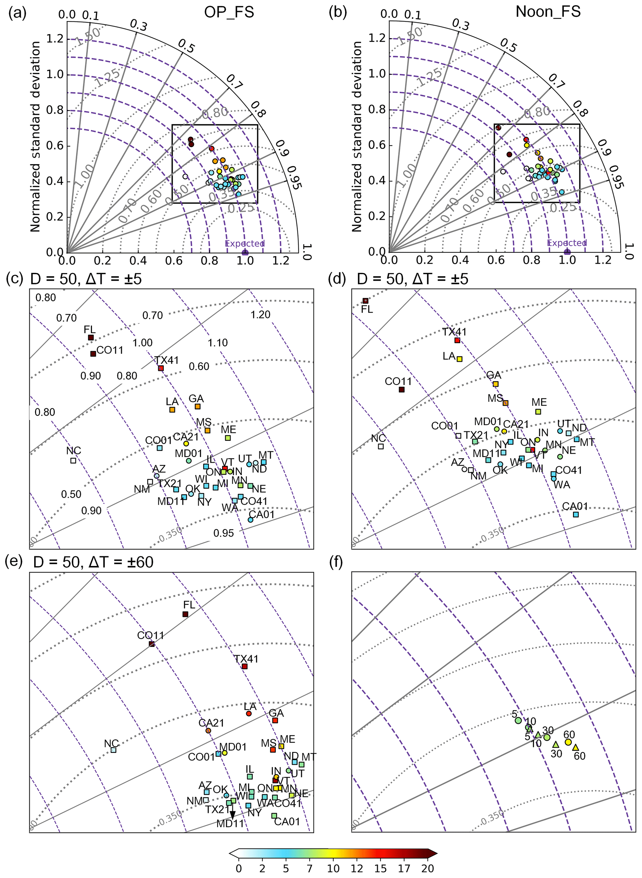
Figure 3Taylor diagrams for evaluating OMI OP_FS EDR (a) and Noon_FS EDR (b) against 31 ground observational sites matched with D=50 km and min, respectively. The circles represent the ground sites and the color at each circle represents the NMB (%). (c, d) are the zoomed-in plot for the boxes in (a, b), respectively. Also, the squares in (c, d) represent sites that have significant NMB at the 95 % confidence level. (e) is the zoomed-in plot for OMI OP_FS EDR evaluation with D=50 km and min. (f) shows the evaluation of OMI OP_FS EDR (triangles) and Noon_FS EDR (circles) with D=50 km and , 10, 30 and 60 min against the ensemble of 31 ground observational sites.
Scatter plots of OMI OP_FS and Noon_FS EDR with all 31 ground observational sites are shown in Fig. 2a and b. Overall, the comparison for OMI OP_FS EDR shows better agreements with the ground data than the comparison for OMI Noon_FS EDR. In both cases, a good linear relationship is found with a correlation coefficient (R) of 0.9 and 0.88 for OMI OP_FS and Noon_FS. This statistically significant correlation (with p<0.01) can also be found at most individual sites, as shown in the Taylor diagrams (Fig. 3a and b). The high correlation found here in the US is consistent with previous work that evaluated OMI EDR in Europe (Buchard et al., 2008; Ialongo et al., 2008). In addition, both OMI OP_FS and Noon_FS EDR were found to overestimate the ground counterparts, with MB of 8 (∼7 %) and 8.9 (∼7 %) mW m−2, respectively. Furthermore, the respective RMSEs are 34.9 and 41.5 mW m−2. The better performance found for OMI OP_FS EDR indicates the uncertainty caused by the assumption of constant atmospheric conditions between OMI overpass time and local solar noon time in the current OMI surface UV algorithm, which has also been highlighted by previous work (Buntoung and Webb, 2010) and will be discussed more in details in Sect. 4.3.
Taylor diagrams in Fig. 3 further illustrate the comparison of OMI OP_FS and Noon_FS EDR with ground measurements at each site. Most individual sites show better performances for OMI overpass time evaluation than local solar noon time evaluation, as expected. For both cases, the performance at each site shows large variation. Site CO11 is located above 3 km and therefore the cloud effects are not corrected, which very likely results in the high bias found in both data comparisons. Thus, CO11 will be excluded in the following discussion. For evaluating OMI OP_FS EDR, the correlation varies from 0.74 (FL01) to 0.95 (CA01), the normalized mean bias varies from −0.54 % (NC01) to 24.5 % (FL01) and the mean bias changes from −0.66 mW m−2 (NC01) to 33.1 mW m−2 (FL01), with 22 sites being statistically significant at the 95 % confidence level. For the OMI Noon_FS EDR comparison, the correlation changes from 0.66 (FL01) to 0.94 (CA01), the NMB increases from −0.39 % (AZ01) to 19.3 % (FL01) and the MB increases from −0.66 mW m−2 (AZ01) to 33.0 mW m−2 (FL01), with 21 sites showing statistical significance at the 95 % confidence level. Also, generally larger standard deviation in the ratio between OMI and ground EDR data is found in the solar noon time comparison (Table S3). Overall, the site at Florida (Fig. 2c and d) shows the worst performance while the site at Davis, CA, shows the best performance.
The various degrees of biases in evaluating OMI EDR reflect the influence of the regional and local differences of air pollution such as aerosol loadings and meteorology across the US. We will use the OMI Noon_FS EDR comparison to discuss the potential regional influence. In the southeast, sites (FL01, LA01, GA01, MS01) show smaller correlation (0.66–0.85) and larger biases – higher than 10 %. The southeast US is characterized by heavy air pollution and high humidity, which would affect clouds and aerosol loadings. Some sites (ME01, MD01, ON01, VT01) in the northeast also shows higher bias above 7 %. The northeast region is also subject to heavy local air pollution. Two sites (IN01, MN01) in the Midwest also show higher bias above 7 %, which could be due to the regional air pollution. A few sites (AZ01, NM01, CA01) in the southwest show smaller bias, which is partially attributed to the dry and less cloudy conditions. In addition, AZ01 and NM01 are located at higher altitude with much cleaner air. As a result, smaller negative biases are found in these two sites. CA21, TX21 and TX41 have biases of 11 %, 7 % and 15 %, which is very likely driven by the local air pollution and possible pollution transport from Mexico. Sites such as UT01, MT01, WA01 and OK01 located in the Pacific Northwest, Rocky Mountains and the central Great Plains region generally have a smaller bias of less than 5 % except for NE01. The spatial variability of OMI EDR biases found in our work is also similar to the work of Xu et al. (2010) which evaluated TOMS spectral UV irradiance with ground measurements at 27 climatological sites from UVMRP in the continental US. These discrepancies can be related to several factors such as the method of collocating OMI data with ground observation spatially and temporally, clouds in the atmosphere, and the assumption of constant atmospheric conditions between OMI overpass time and local solar noon time, which are discussed in the following sections.
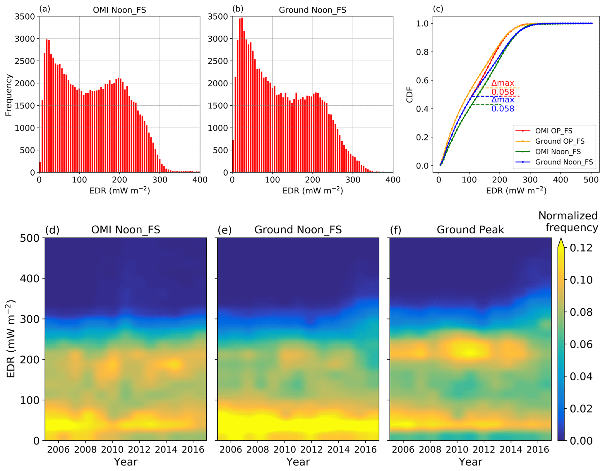
Figure 4Frequency of the surface EDR at the solar noon time for OMI (a) and 31 ground observational sites (b) for year 2005–2017. All the data pairs are matched with D=50 km and min. (c) shows the cumulative distribution functions (CDFs) of surface EDR from both OMI and 31 ground observational sites over 2005–2017. The maximum differences between OMI and ground observational CDFs are shown in the horizontal dashed lines and their values are shown as the labels. (d–f) are contour plots of normalized frequency of surface EDR from OMI and ground Noon_FS EDR as well as ground peak for 31 ground sites. The ground peak refers to the highest dose rate found in a day at each site. The normalized frequency is calculated as follows: first, the surface EDRs from both OMI and ground observation are binned by 25 mW m−2 for each year and then normalized by the total number of data points for each year. A smooth effect at the contour line was also performed.
To further show how well OMI surface EDR represents the ground observational EDR, the frequency of both OMI and ground EDR is shown (Fig. 4). First, we find that the distribution of surface EDR at solar noon time from both OMI and ground observational data shows two peaks, one around 20 mW m−2 and the other one around 200 mW m−2. A similar distribution with two peaks is also found for OMI and ground EDR at overpass time, which are not shown here. These two peaks are largely due to the SZA effects (Wang and Christopher, 2006). Figure 4c shows the calculated CDFs for OMI and ground OP_FS and Noon_FS EDR as well as the maximum difference between EDRs at the corresponding time. The critical value for both comparisons is 0.087 to verify that the two CDFs show a good fit at the 99 % confidence level. From Fig. 4c, we can see that both of the maximum differences are smaller than the critical values at the 99 % confidence level. Therefore, the null hypothesis (OMI surface EDR and ground-observed EDR were drawn from the same distribution) will not be rejected. This good fit between OMI and ground EDR distribution for both solar noon time and overpass time again confirms the good correlation found between these two datasets.
In order to better understand the variability of surface UV, we also study the peak UV frequency inferred from ground observation along with OMI and ground Noon_FS EDR frequency. The peak UV is calculated as the highest dose rate found in a day at each site. As seen in Fig. 4d–f, all of the OMI Noon_FS, ground Noon_FS and ground peak data show a high frequency at the lower end of surface EDR (<100 mW m−2), which also reflects the smaller peak found in Fig. 4a and b. Moreover, this high frequency of occurrence persisted from 2005 to 2017 for all datasets. In addition, both OMI and ground Noon_FS EDR show another high frequency of surface EDR around 200 mW m−2 corresponding to the other peak in Fig. 4a and b. However, the OMI Noon_FS data show a stronger and more persistent frequency than that of ground Noon_FS data. Additionally, the ground peak values find a high frequency around ∼220 mW m−2 (Fig. 4f). The high-frequency occurrence of ∼220 mW m−2 in ground measurements prevailed until 2015 and, at the same time, we find the frequency of higher surface EDR from ground peak of ∼300 mW m−2 starts to increase around 2014. This increase in the occurrence of peak UV irradiance could have potential implications for human exposure and subsequent health effects, which is beyond the scope of this study. The contrast between Fig. 4e and f suggests that the peak of surface UV irradiance may not always occur during the solar noon time, reflecting the change of meteorology during the day and suggesting the need for multiple observations per day.
4.2 Impacts of spatial collocation and temporal averaging
Table S2 summarizes the regression statistics and other validation statistics of evaluating OMI OP_FS and Noon_FS EDR with different spatial collocation distances (D) and temporal averaging windows (ΔT), respectively. We find that the length of temporal averaging windows seems to play a more important role in the overall comparison results than the spatial colocation distance. Figure 3c–e shows that most of the dots representing the OMI OP_FS EDR evaluation on the Taylor diagram move closer to the expected point as ΔT increases from ±5 to ±60 min. The same progression is also found for the OMI Noon_FS EDR evaluation, which is not shown here. Figure 3f further shows that the correlation of the OMI OP_FS and Noon_FS EDR evaluation increases as ΔT changes from ±5 to ±60 min. In addition, the RMSE decreases by 12 % for both data comparisons when ΔT increases from ±5 to ±60 min. The improvement with a longer temporal averaging window for overpass time under full sky is also found by Zempila et al. (2016).
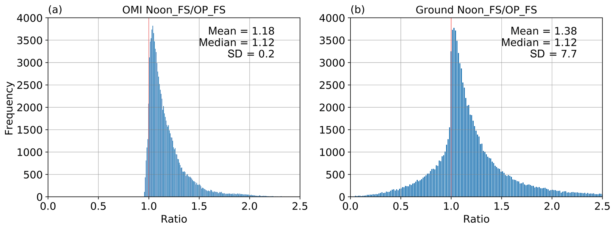
Figure 5Frequency of the EDR ratio of Noon_FS ∕ OP_FS. (a, b) are for the OMI and ground ratio, respectively. All the data pairs are matched with D=50 km and 5 min for the 31 ground sites.
4.3 Impacts of the assumption of constant atmospheric conditions
As described in Sect. 2.1, the current surface UV algorithm assumes the same atmospheric conditions at OMI overpass time and the local solar noon time regarding cloudiness, total column ozone and atmospheric aerosol loadings but with different SZAs. However, this assumption may not hold all the time for the real atmosphere. We take the ratio between Noon_FS and OP_FS EDR (Noon_FS ∕ OP_FS) from both OMI and ground data as an indicator of the variation of atmospheric conditions between these two times. Figure 5 shows the frequency of this ratio from both OMI and ground data obtained with D=50 km and min. Both ratios show the same median of 1.12; however, the ground ratio shows a larger mean (1.38 vs. 1.18) and standard deviation. The mean of 1.18 in the OMI ratio data reflects the effects of SZAs while the larger mean of 1.38 obtained from ground data implies the impacts from air pollution and meteorology. The scatter plot (Fig. 6a) of the ground ratio and OMI ratio further shows the discrepancy. Overall, approximately 95 % of the OMI data fall into the area with the ratio greater than 1, again reflecting the large effects of SZA, while 22 % of ground data show a ratio smaller than 1, reflecting the influence of short-term variability of local atmospheric conditions such as clouds, which can override the effect of SZA. The frequency of ground ratio less than 1 also varies at individual sites (Table S3). We find that the frequency at site AZ01, CA01, CA21 and NM01 is among the smallest, below 15 %. As mentioned in Sect. 4.1, these sites are located in the southwest with prevailing dry climate and as a result the effects of clouds are much smaller. Also, sites AZ01 and NM01 are located at higher altitude with cleaner air and, subsequently, the effects from air pollution are minimal. The frequency exceeds 15 % at the rest of the sites, with VT01 showing the maximum of ∼32 %, which are most likely affected by air pollution. These findings indicate the current OMI surface UV algorithm may not fully capture the real atmosphere by assuming constant atmospheric conditions between satellite overpass time and the local solar noon time.
We further investigate the possible seasonal effects on this ratio. As can be seen in Fig. 6b, the mean and median ratio (Noon_FS ∕ OP_FS) from OMI are greater than those from the ground observational data throughout the year except for January, which again indicates the potential overestimation of OMI Noon_FS EDR using constant atmospheric conditions. Furthermore, the discrepancy between these two ratios stays consistent in the spring and summer time. The smaller SZA in the summer time would have relatively smaller effects and the difference in these ratios could be largely affected by the varying atmospheric conditions between local solar noon time and OMI overpass time. However, this discrepancy becomes larger in the fall and winter time, which could be the result of the elevated SZA towards winter time in North America to some extent. The larger SZA (>70∘) in the colder times could increase the radiation path in the atmosphere, which would thereby amplify the atmospheric interaction with the solar radiation. Besides, other seasonal variables such as the climatological albedo used in the current OMI surface UV algorithm could potentially play a role in the deviation between OMI and ground data. In addition, the ratio from both OMI and ground observational data shows larger variation in the fall and winter season than its respective summer season, implying the impacts of the SZA seasonal variation on both OMI and observational data.
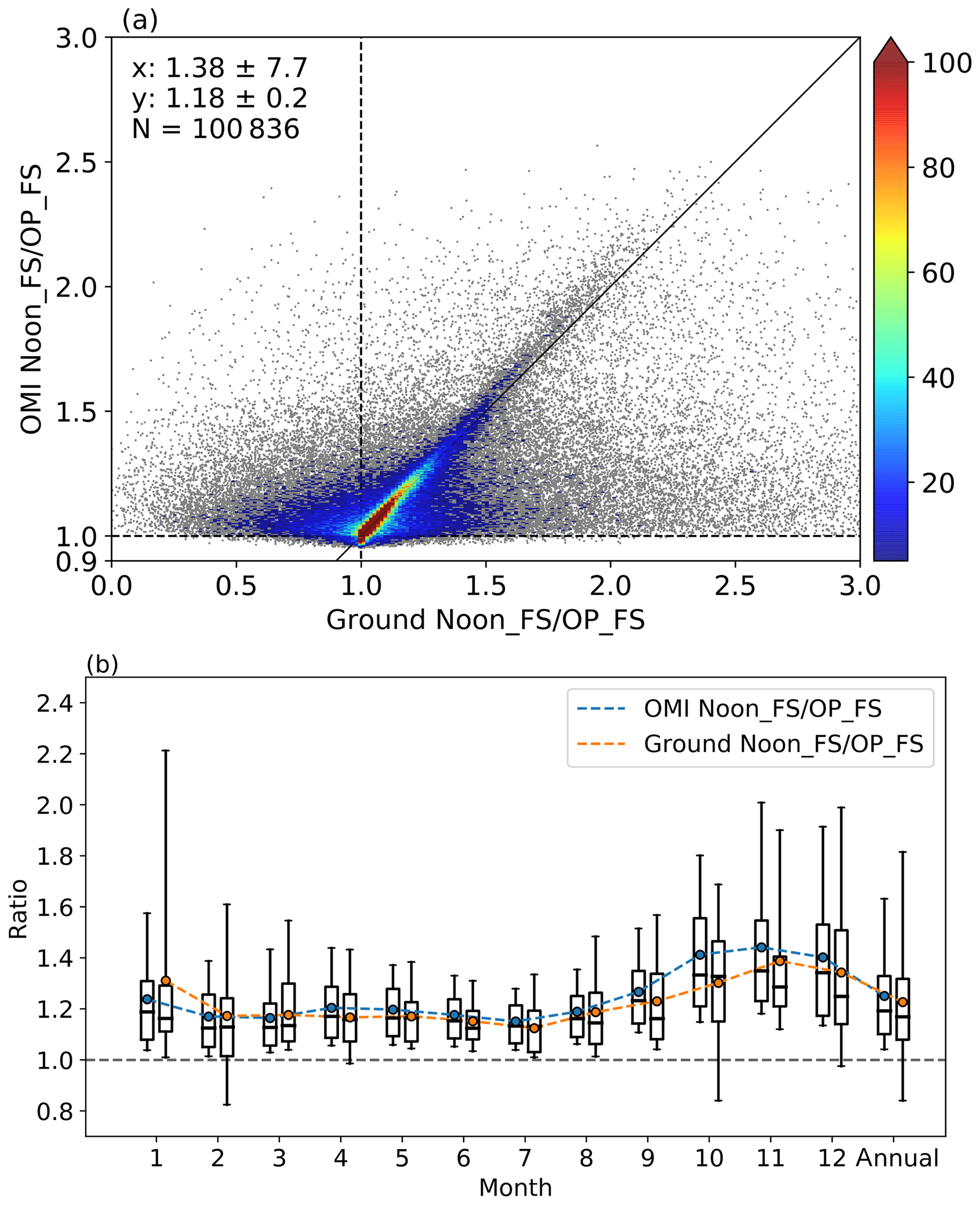
Figure 6(a) is the scatter plot of the EDR ratio of Noon_FS ∕ OP_FS between OMI and ground measurements for 31 sites. All the data pairs are matched with D=50 km and min. Also shown on the scatter plot are the number of collocated data points (N), the density of points (the color bar) and the 1:1 line (the solid black line). Note the scale difference between x and y axis. (b) is the monthly EDR ratio of Noon_FS ∕ OP_FS from OMI (blue) and ground measurements (orange) for 31 sites. The box–whisker plots show the 5th and 95th percentiles (whisker), the interquartile range (box), the median (black line) and the mean (the dots).
The SZA seasonal variation could subsequently affect the difference between OMI and ground data, which will be analyzed in this section. Several previous studies have investigated the effects of SZA on the difference between OMI and ground observational irradiance. Buchard et al. (2008) found that OMI spectral UV irradiance on clear-sky days showed a larger discrepancy at SZA greater than 65∘. Kazadzis et al. (2009a) found no systematic dependence of the difference between OMI and ground observational spectral UV irradiance on SZA. By sorting data based on cloud and aerosol conditions, Antón et al. (2010) showed that the relative difference between OMI and ground irradiance decreases modestly with SZA for all-sky conditions except for days with high aerosol loadings. Zempila et al. (2016) suggested a small dependence of the ratio (OMI ∕ ground UV irradiance) on SZA under both clear-sky and all-sky conditions. For the all-sky condition, the ratio increases steadily with increasing SZA up to 50∘ and becomes larger than 1 after 50∘. Similar to these previous works, we also find that the impacts of SZA could cause various levels of biases in evaluating OMI EDR depending on locations (Fig. S1 in the Supplement and Fig. 7). As seen from Fig. S1, the mean bias for the OMI Noon_FS EDR comparison is larger than the OP_FS comparison at most sites for both smaller SZAs (SZA < 50∘) and larger SZAs (50∘ < SZA < 75∘). For some sites in higher latitudes such as ND01 and WA01, the mean biases at larger SZAs are smaller than those at smaller SZAs because the frequency of negative bias increases at larger SZAs.
Clouds also play an important role in the difference between OMI and ground observational UV irradiance. Buchard et al. (2008) found that the relative difference between OMI and ground EDR was associated with COT at 360 nm retrieved from OMI and the difference is more appreciable for large COT. Tanskanen et al. (2007) showed that the distribution of the OMI and ground EDD ratio widens with increasing COT. Antón et al. (2010) used OMI-retrieved LER at 360 nm as a proxy for cloudiness and showed that the relative difference of OMI and ground EDR increased largely at higher LER values. Here, we find that the relative bias for OMI OP_FS EDR is more obvious at larger COT values as well (Fig. 7c). In addition, the noise of the bias gets larger at higher COT values. One of the reasons could be that the OMI surface UV algorithm uses the average of a pixel to represent the cloudiness in that specific pixel. In reality, the spatial distribution of cloudiness in that pixel could vary a lot, which could result in the large difference in surface UV irradiance between the OMI pixel and the ground observational site.
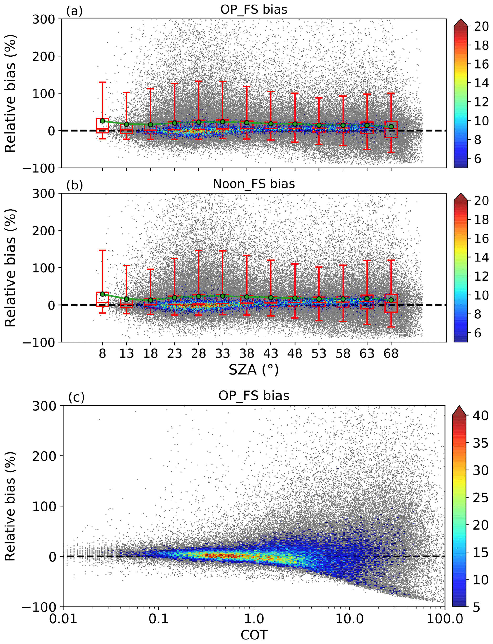
Figure 7Scatter plots of the relative bias (%) between OMI and ground observational EDR and the OMI overpass time SZA or COT (360 nm). (a, c) are for OMI OP_FS bias while (b) is for Noon_FS bias. All the data pairs are matched with D=50 km and min for 31 ground sites. The box–whisker plot of the bias on (a, b) is based on the binned SZA using a bin size of 5∘. The box–whisker plots show the 5th and 95th percentiles (whisker), the interquartile range (box), the median (red line) and the mean (green dots).
4.4 Trend analysis
EDR is the weighted solar irradiance from 300 to 400 nm which covers the UVB range that is greatly affected by the atmospheric ozone column. In addition, both UVA and UVB could be affected by the cloud cover and aerosol loadings in the atmosphere. Thus, trends in surface EDR could be a result of the combined effects of the aforementioned different factors and it would be challenging to attribute the trend to any individual factor quantitatively. Therefore, we focus on providing a descriptive summary of surface EDR trends derived from both OMI and ground observation.
We first analyze the surface EDR trend using OMI level 3 data. We find that OMI full-sky solar noon EDR data show a positive trend in most of the places; but the only significant trend (95 % confidence level) was found in parts of the northeastern US (Fig. 8b). A similar distribution of the trend is found in OMI level 3 full-sky spectral irradiance at 310 nm (Fig. 8d). We also analyzed the trend of OMI level 3 clear-sky EDR and total column ozone amount (Fig. S2c) and found no significant trend in either dataset. This could suggest that the contribution of ozone column to the estimated trend of OMI full-sky EDR is minimal. Furthermore, significant trends in OMI level 3 full-sky spectral irradiance at 380 nm are found in the northeast (Fig. 8e) and no significant trends of OMI level 3 COT are found (Fig. S2b), indicating the estimated trend could be largely induced by the aerosols.
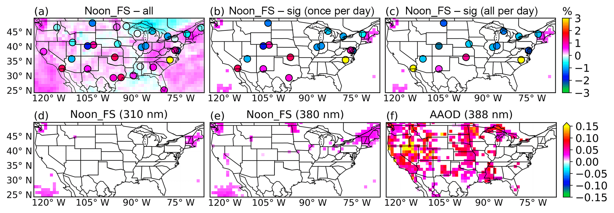
Figure 8(a) is the distribution of the OMI level 3 solar noon time full-sky EDR trend over 2005–2017 overlaid with the trend at 31 ground sites calculated with D=50 km and min around local solar noon time. (b) is the same as (a) but only showing the areas and sites that are significant at the 95 % confidence level. (c) shows the distribution of the trend at ground sites (significant at the 95 % confidence level), computed with D=50 km and temporally averaging all the data available in a day. (d, e) show the areas with significant trends of OMI level 3 solar noon time full-sky spectral irradiance at 310 and 380 nm, respectively. (a–e) share the same color bar and the trend shown is the percentage change (%) per year. (f) shows the significant trend at the 95 % confidence level for OMI level 3 AAOD at 388 nm. The trend is calculated as 100 × AAOD/year.
In contrast to trends derived from OMI data, ground observation shows different trend patterns using two different sampling methods. For both methods, only months with more than 20 days of data are used for trend analysis and considered missing values otherwise. The first method is to average the ground observational data with D=50 km and min around local solar noon time, denoted as once-per-day sampling. A total of 16 of 31 sites is found to have significant trends at the 95 % confidence level (Fig. 8b). Seven sites have positive trends while the rest of the 9 sites show negative trends. The second method averages all the data in a day at each site, hereby referred to as all-per-day sampling. We find that this method results in 14 sites with significant trends at the 95 % confidence level (Fig. 8c). Only 4 of the 14 sites have positive trends, with the rest of the sites showing negative trends.
Both methods (e.g., once per day and all per day) find significant negative trends for sites in the northeast and the Ohio River Valley region with the all-per-day method showing smaller trends. Using the site IL01 as an example, Fig. S3 illustrates the difference between these two sampling methods. Both methods could capture the seasonal variation of the surface EDR; however, the magnitude of all-per-day sampling EDR is about 3 times smaller than that of the once-per-day sampling, which is anticipated because the all-per-day average is smaller than the once-per-day measurement around noon time. By averaging all the daytime data, the all-per-day sampling method smooths out the atmospheric conditions throughout the day. In contrast, the estimated trend of OMI Noon_FS EDR at this site is not significant. In addition, the ground measurements show increasing trends in the southern Great Plains (Texas and Oklahoma), while we find significant increasing trends from OMI AAOD at 388 nm (Fig. 8f) but no significant trends of OMI AOD at 388 nm (Fig. S2a) are found in these regions. Zhang et al. (2017) also found significant positive trends of OMI AAOD in this region, largely caused by dust AAOD. However, the magnitude of these trends derived from ground measurements is within the measurement uncertainty range. Given these uncertainties in the surface measurements, no coherent and scientifically sound trend can be drawn from OMI data products for EDR, AOD, AAOD, COT, and column ozone amount (Fig. S2c) and ground observations.
In this study, we evaluated the OMI surface erythemal irradiance at overpass time and solar noon time for the period of 2005–2017 with 31 UVMRP ground sites in the continental US. The OMI surface Noon_FS EDR shows a meridional gradient with the EDR increasing from ∼80 mW m−2 in the northern US to ∼203 mW m−2 in the southern US. The ground observational data could capture this gradient well with EDR increasing from ∼73 mW m−2 in the northern US to a maximum of ∼190 mW m−2 at the southern sites.
The evaluation for OMI overpass time EDR shows better agreement with ground measurements than that for solar noon time comparison. Both OMI OP_FS and Noon_FS EDR comparisons show good correlation with the counterparts from ground-based measurements, with R=0.90 and 0.88, respectively, when inter-comparison is matched with D=50 km and min; the correlation further increases as ΔT increases to 30 min or 1 h. Both OMI OP_FS and Noon_FS EDR overestimate the ground measurements by 8.0 and 8.9 mW m−2, respectively, and their RMSEs are 34.9 and 41.5 mW m−2. The biases also show large spatial variability. For both OMI OP_FS and Noon_FS EDR comparisons, the NMB varies from −1 % to 20 % while the OMI Noon_FS comparison shows larger MB. This suggests that the atmospheric condition does not stay consistent even within an hour, underscoring the importance of geostationary satellite measurements. The relatively large bias and RMSE in magnitude for OMI Noon_FS EDR suggest the importance of accounting for the variation of atmospheric conditions between solar noon and satellite overpass time, which cannot be resolved by polar-orbiting satellite measurements but future geostationary satellites such as TEMPO (Tropospheric Emissions: Monitoring of Pollution) (Zoogman et al., 2017), Sentinel-4 (Ingmann et al., 2012; Veihelmann et al., 2015) and GEMS (Geostationary Environmental Monitoring Spectrometer) should be able to resolve this issue.
We also extended the evaluation of OMI and ground EDR by comparing the PDFs and CDFs as well as considering the peak UV density. First, both OMI and ground EDR distributions show two peaks, one around 20 mW m−2 and another around 200 mW m−2, mainly related to larger and smaller SZAs, respectively. The K–S test shows that the OMI and ground EDR are from the same sample distribution at the 99 % confidence level. Both OMI Noon_FS EDR, ground Noon_FS EDR and ground peak show the high-frequency occurrence of the smaller peak (∼20 mW m−2) over the period of 2005–2017. However, the other high-frequency occurrence of ground noontime EDR (∼200 mW m−2) is not consistent with the high frequency found in ground daily-peak values (∼220 mW m−2), implying that the peak UV values in a day may not always occur at the local solar noon time, thus highlighting the necessity for finer temporal resolution data.
Ground-based continuous measurements were used to show the effects of atmospheric variation on surface EDR. The ratio of OMI Noon_FS ∕ OP_FS EDR is greater than 1 for 95 % of the data points, while the ratio derived from the ground-based data has a Gaussian distribution, with 22 % of the data smaller than 1 and a mean value of 1.38. This means that the assumption of a consistent cloudiness, column ozone amount and aerosol loadings between these two times would lead to large positive bias in the estimates of surface UV at solar noon time, which is revealed in this study. Furthermore, we find that the OMI OP_FS EDR bias shows various levels of dependence on the SZAs. Additionally, the OMI OP_FS EDR bias shows slight dependence on COT. The error distribution of the bias gets much wider at larger COT values. This error statistic suggests the importance of multiple scattering by aerosols and clouds in the radiative transfer model, which is overlooked in the radiative transfer calculation for the current OMI's lookup table approach to estimate surface UV. Lastly, because the current work deals with erythemal irradiance data, the comparison of satellite and ground observational erythemal irradiance at both satellite overpass and local solar noon time could only provide us the overall combined effects of the varying atmospheric conditions between these two times. The limitation is that it would not provide quantitative information of the individual effect of the atmospheric condition such as aerosol loadings on the transferability from satellite overpass time to the local solar noon time. Additional comparison of spectral irradiance such as in the work of Xu et al. (2010) would help identify the specific cause. The current work by focusing on only erythemal irradiance still shows the short-time variability from satellite overpass time and local solar noon time. Again, future geostationary satellite data (TEMPO and GEMS) combined with ground observational data would help better understand the temporal and spatial variability of surface UV irradiance.
Lastly, we investigated the surface UV trend from both OMI and ground observational data. The trend from ground data depends on sampling method. The once-per-day sampling at noon time shows larger spatial variability in the magnitude and signs of the trend while the all-per-day sampling shows less variation in the magnitude. But, over the northeastern US, both methods yield negative trends from the surface observations, while significant positive trends were found from OMI full-sky data during solar noon time. Furthermore, ground measurements and OMI data show significant trends of surface UV in the southern Great Plains. However, the values of trends are within the surface measurement uncertainties. Overall, there are no scientifically sound and coherent trends among OMI data for aerosols, clouds and ozone that can explain the surface UV trends revealed either by OMI or ground-based estimates; these data also cannot reconcile trend differences between the two estimates. Further studies of the trends in OMI and ground-based spectral irradiances may help reveal more information of the effects of total ozone amount on surface UV irradiance. Also, detailed studies of aerosols trends may provide extra insights on the effects of aerosols on the surface UV trends.
OMI data are downloaded from https://disc.gsfc.nasa.gov (last access: 30 January 2019). Ground observational data are download from https://uvb.nrel.colostate.edu/UVB/uvb-dataAccess.jsf (last access: 21 January 2019). We thank both the OMI team and UVMRP for providing the data.
The supplement related to this article is available online at: https://doi.org/10.5194/acp-19-2165-2019-supplement.
HZ, LCG, CD and JZ prepared and analyzed the data. JW, YL and NAK helped with the data analysis. JW, HZ and JZ designed the research. All authors participated in the process of writing the manuscript.
The authors declare that they have no conflict of interest.
The research was funded by NASA's Aura satellite program (managed by
Kenneth W. Jucks), Applied Sciences Program (grant no. NNX14AG01G, managed by John A. Haynes), and
Atmospheric Composition Modeling and Analysis Program (ACMAP managed by Richard Eckman).
The authors thank the OMI team for providing the surface UV and
aerosol products, which can be downloaded from the NASA Goddard Earth
Sciences (GES) Data and Information Services Center (DISC) (https://disc.gsfc.nasa.gov,
last access: 30 January 2019). We also thank the UVMRP for the ground
observational UV data, which are available at https://uvb.nrel.colostate.edu/UVB/uvb-dataAccess.jsf
(last access: 21 January 2019). We appreciate
Antti Arola from the Finnish Meteorological Institute for the helpful discussion
on the OMI surface UV algorithm.
Edited by: Stelios Kazadzis
Reviewed by: three anonymous referees
Andrady, A. L., Aucamp, P. J., Austin, A., Bais, A. F., Ballaré, C. L., Barnes, P. W., Bernhard, G. H., Bornman, J. F., Caldwell, M. M., de Gruijl, F. R., Erickson III, D. J., Flint, S. D., Gao, K., Gies, P., Häder, D.-P., Ilyas, M., Longstreth, J., Lucas, R., Madronich, S., McKenzie, R. L., Neale, R., Norval, M., Pandy, K. K., Paul, N. D., Rautio, M., Redhwi, H., Robinson, S. A., Rose, K., Shao, M., Sinha, R. P., Solomon, K. R., Sulzberger, B., Takizawa, Y., Tang, X., Torikai, A., Tourpali, K., van der Leun, J. C., Wängberg, S.-Å., Williamson, C. E., Wilson, S. R., Worrest, R. C., Young, A. R., and Zepp, R. G.: Environmental effects of ozone depletion and its interactions with climate change: 2014 assessment Executive summary, Photochem. Photobiol. Sci., 14, 14–18, https://doi.org/10.1039/C4PP90042A, 2015.
Antón, M., Cachorro, V., Vilaplana, J., Toledano, C., Krotkov, N., Arola, A., Serrano, A., and Morena, B.: Comparison of UV irradiances from Aura/Ozone Monitoring Instrument (OMI) with Brewer measurements at El Arenosillo (Spain) – Part 1: Analysis of parameter influence, Atmos. Chem. Phys., 10, 5979–5989, https://doi.org/10.5194/acp-10-5979-2010, 2010.
Arola, A., Kazadzis, S., Krotkov, N., Bais, A., Gröbner, J., and Herman, J. R.: Assessment of TOMS UV bias due to absorbing aerosols, J. Geophys. Res.-Atmos., 110, D23211, https://doi.org/10.1029/2005JD005913, 2005.
Arola, A., Kazadzis, S., Lindfors, A., Krotkov, N., Kujanpää, J., Tamminen, J., Bais, A., di Sarra, A., Villaplana, J. M., Brogniez, C., Siani, A. M., Janouch, M., Weihs, P., Webb, A., Koskela, T., Kouremeti, N., Meloni, D., Buchard, V., Auriol, F., Ialongo, I., Staneck, M., Simic, S., Smedley, A., and Kinne, S.: A new approach to correct for absorbing aerosols in OMI UV, Geophys. Res. Lett., 36, L22805, https://doi.org/10.1029/2009GL041137, 2009.
Bernhard, G. and Seckmeyer, G.: Uncertainty of measurements of spectral solar UV irradiance, J. Geophys. Res.-Atmos., 104, 14321–14345, 1999.
Bernhard, G., Arola, A., Dahlback, A., Fioletov, V., Heikkilä, A., Johnsen, B., Koskela, T., Lakkala, K., Svendby, T., and Tamminen, J.: Comparison of OMI UV observations with ground-based measurements at high northern latitudes, Atmos. Chem. Phys., 15, 7391–7412, https://doi.org/10.5194/acp-15-7391-2015, 2015.
Bigelow, D. S., Slusser, J., Beaubien, A., and Gibson, J.: The USDA ultraviolet radiation monitoring program, B. Am. Meteorol. Soc., 79, 601–615, 1998.
Bornman, J. F. and Teramura, A. H.: Effects of ultraviolet-B radiation on terrestrial plants, in: Environmental UV photobiology, Springer, Boston, MA, 427–471, 1993.
Boys, B., Martin, R., Van Donkelaar, A., MacDonell, R., Hsu, N., Cooper, M., Yantosca, R., Lu, Z., Streets, D., and Zhang, Q.: Fifteen-year global time series of satellite-derived fine particulate matter, Environ. Sci. Technol., 48, 11109–11118, 2014.
Buchard, V., Brogniez, C., Auriol, F., Bonnel, B., Lenoble, J., Tanskanen, A., Bojkov, B., and Veefkind, P.: Comparison of OMI ozone and UV irradiance data with ground-based measurements at two French sites, Atmos. Chem. Phys., 8, 4517–4528, https://doi.org/10.5194/acp-8-4517-2008, 2008.
Buntoung, S. and Webb, A.: Comparison of erythemal UV irradiances from Ozone Monitoring Instrument (OMI) and ground-based data at four Thai stations, J. Geophys. Res.-Atmos., 115, D18215, https://doi.org/10.1029/2009JD013567, 2010.
Cabrera, S., Ipiña, A., Damiani, A., Cordero, R. R., and Piacentini, R. D.: UV index values and trends in Santiago, Chile (33.5∘ S) based on ground and satellite data, J. Photochem. Photobiol. B, 115, 73–84, 2012.
Caldwell, M., Teramura, A. H., Tevini, M., Bornman, J., Björn, L. O., and Kulandaivelu, G.: Effects of increased solar ultraviolet-radiation on terrestrial plants, Ambio, 24, 166–173, 1995.
Cede, A., Luccini, E., Nuñez, L., Piacentini, R. D., Blumthaler, M., and Herman, J. R.: TOMS-derived erythemal irradiance versus measurements at the stations of the Argentine UV Monitoring Network, J. Geophys. Res.-Atmos., 109, D08109, https://doi.org/10.1029/2004JD004519, 2004.
Chubarova, N. Y., Yurova, A. Y., Krotkov, N. A., Herman, J. R., and Bhartia, P. K.: Comparisons between ground measurements of UV irradiance 290 to 380 nm and TOMS UV estimates over Moscow for 1979–2000, Opt. Eng., 41, 3070–3081, 2002.
Deirmendjian, D.: Electromagnetic scattering on spherical polydispersions, Rand Corp, Santa Monica, CA, 1969.
Eck, T. F., Bhartia, P. K., and Kerr, J. B.: Satellite estimation of spectral UVB irradiance using TOMS derived total ozone and UV reflectivity, Geophys. Res. Lett., 22, 611–614, https://doi.org/10.1029/95GL00111, 1995.
Eide, M. J. and Weinstock, M. A.: Association of UV index, latitude, and melanoma incidence in nonwhite populations – US Surveillance, Epidemiology, and End Results (SEER) Program, 1992 to 2001, Arch. Dermatol., 141, 477–481, 2005.
Farman, J. C., Gardiner, B. G., and Shanklin, J. D.: Large losses of total ozone in Antarctica reveal seasonal ClOx∕NOx interaction, Nature, 315, 207–210, 1985.
Fioletov, V., Bodeker, G., Miller, A., McPeters, R., and Stolarski, R.: Global and zonal total ozone variations estimated from ground-based and satellite measurements: 1964–2000, J. Geophys. Res.-Atmos., 107, 4647, https://doi.org/10.1029/2001JD001350, 2002.
Gao, W., Davis, J. M., Tree, R., Slusser, J. R., and Schmoldt, D.: An ultraviolet radiation monitoring and research program for agriculture, in: UV Radiation in Global Climate Change, Springer, Berlin, Heidelberg, 205–243, 2010.
Herman, J., Krotkov, N., Celarier, E., Larko, D., and Labow, G.: Distribution of UV radiation at the Earth's surface from TOMS-measured UV-backscattered radiances, J. Geophys. Res.-Atmos., 104, 12059–12076, 1999.
Ialongo, I., Casale, G. R., and Siani, A. M.: Comparison of total ozone and erythemal UV data from OMI with ground-based measurements at Rome station, Atmos. Chem. Phys., 8, 3283–3289, https://doi.org/10.5194/acp-8-3283-2008, 2008.
Ingmann, P., Veihelmann, B., Langen, J., Lamarre, D., Stark, H., and Courrèges-Lacoste, G. B.: Requirements for the GMES Atmosphere Service and ESA's implementation concept: Sentinels-4/-5 and-5p, Remote Sens. Environ., 120, 58–69, 2012.
Janjai, S., Wisitsirikun, S., Buntoung, S., Pattarapanitchai, S., Wattan, R., Masiri, I., and Bhattarai, B.: Comparison of UV index from Ozone Monitoring Instrument (OMI) with multi-channel filter radiometers at four sites in the tropics: effects of aerosols and clouds, Int. J. Climatol., 34, 453–461, 2014.
Kalliskota, S., Kaurola, J., Taalas, P., Herman, J. R., Celarier, E. A., and Krotkov, N. A.: Comparison of daily UV doses estimated from Nimbus 7/TOMS measurements and ground-based spectroradiometric data, J. Geophys. Res.-Atmos., 105, 5059–5067, 2000.
Kazadzis, S., Bais, A., Arola, A., Krotkov, N., Kouremeti, N., and Meleti, C.: Ozone Monitoring Instrument spectral UV irradiance products: comparison with ground based measurements at an urban environment, Atmos. Chem. Phys., 9, 585–594, https://doi.org/10.5194/acp-9-585-2009, 2009a.
Kazadzis, S., Bais, A., Balis, D., Kouremeti, N., Zempila, M., Arola, A., Giannakaki, E., Amiridis, V., and Kazantzidis, A.: Spatial and temporal UV irradiance and aerosol variability within the area of an OMI satellite pixel, Atmos. Chem. Phys., 9, 4593–4601, https://doi.org/10.5194/acp-9-4593-2009, 2009b.
Kazantzidis, A., Bais, A., Gröbner, J., Herman, J., Kazadzis, S., Krotkov, N., Kyrö, E., Den Outer, P., Garane, K., and Görts, P.: Comparison of satellite-derived UV irradiances with ground-based measurements at four European stations, J. Geophys. Res.-Atmos., 111, D13207, https://doi.org/10.1029/2005JD006672, 2006.
Kimlin, M. G., Slusser, J. R., Schallhorn, K. A., Lantz, K. O., and Meltzer, R. S.: Comparison of ultraviolet data from colocated instruments from the US EPA Brewer Spectrophotometer Network and the US Department of Agriculture UV-B Monitoring and Research Program, Opt. Eng., 44, 041009, https://doi.org/10.1117/1.1885470, 2005.
Koh, H. K., Geller, A. C., Miller, D. R., Grossbart, T. A., and Lew, R. A.: Prevention and early detection strategies for melanoma and skin cancer: current status, Arch. Dermatol., 132, 436–443, 1996.
Krotkov, N. A., Bhartia, P. K., Herman, J. R., Fioletov, V., and Kerr, J.: Satellite estimation of spectral surface UV irradiance in the presence of tropospheric aerosols: 1. Cloud-free case, J. Geophys. Res.-Atmos., 103, 8779–8793, https://doi.org/10.1029/98JD00233, 1998.
Krotkov, N. A., Herman, J. R., Bhartia, P. K., Fioletov, V., and Ahmad, Z.: Satellite estimation of spectral surface UV irradiance: 2. Effects of homogeneous clouds and snow, J. Geophys. Res.-Atmos., 106, 11743–11759, https://doi.org/10.1029/2000JD900721, 2001.
Krotkov, N. A., Herman, J. R., Bhartia, P. K., Seftor, C. J., Arola, A., Kaurola, J., Kalliskota, S., Taalas, P., and Geogdzhayev, I. V.: Version 2 total ozone mapping spectrometer ultraviolet algorithm: Problems and enhancements, Opt. Eng., 41, 3028–3040, 2002.
Krzyścin, J. W., Sobolewski, P. S., Jarosławski, J., Podgórski, J., and Rajewska-Więch, B.: Erythemal UV observations at Belsk, Poland, in the period 1976–2008: Data homogenization, climatology, and trends, Acta Geophysica, 59, 155–182, 2011.
Lakkala, K., Asmi, E., Meinander, O., Hamari, B., Redondas, A., Almansa Rodríguez, A. F., Carreño Corbella, V., Ochoa, H., and Deferrari, G.: Observations from the NILU-UV Antarctic network since 2000, 2014.
Lantz, K. O., Disterhoft, P., DeLuisi, J. J., Early, E., Thompson, A., Bigelow, D., and Slusser, J.: Methodology for deriving clear-sky erythemal calibration factors for UV broadband radiometers of the US Central UV Calibration Facility, J. Atmos. Ocean. Tech., 16, 1736–1752, 1999.
Lemus-Deschamps, L. and Makin, J. K.: Fifty years of changes in UV Index and implications for skin cancer in Australia, Int. J. Biometeorol., 56, 727–735, 2012.
Levelt, P. F., van den Oord, G. H., Dobber, M. R., Malkki, A., Visser, H., de Vries, J., Stammes, P., Lundell, J. O., and Saari, H.: The ozone monitoring instrument, IEEE T. Geosci. Remote, 44, 1093–1101, 2006.
McKenzie, R., Seckmeyer, G., Bais, A., Kerr, J., and Madronich, S.: Satellite retrievals of erythemal UV dose compared with ground-based measurements at northern and southern midlatitudes, J. Geophys. Res.-Atmos., 106, 24051–24062, 2001.
McKenzie, R., Smale, D., and Kotkamp, M.: Relationship between UVB and erythemally weighted radiation, Photochem. Photobiol. Sci., 3, 252–256, 2004.
McKenzie, R., Bodeker, G., Scott, G., Slusser, J., and Lantz, K.: Geographical differences in erythemally-weighted UV measured at mid-latitude USDA sites, Photochem. Photobiol. Sci., 5, 343–352, 2006.
McKinlay, A. and Diffey, B.: A reference action spectrum for ultraviolet erythema in human skin, CIE J., 6, 17–22, 1987.
Pandey, P., Gillotay, D., and Depiesse, C.: Climatology of ultra violet (UV) irradiance at the surface of the earth as measured by the Belgian UV radiation monitoring network, in: Proceedings of Living Planet Symposium, 9–13 May 2016, Prague, Czech Republic, 9–13, 2016.
Sabburg, J., Rives, J., Meltzer, R., Taylor, T., Schmalzle, G., Zheng, S., Huang, N., Wilson, A., and Udelhofen, P.: Comparisons of corrected daily integrated erythemal UVR data from the US EPA/UGA network of Brewer spectroradiometers with model and TOMS-inferred data, J. Geophys. Res.-Atmos., 107, 4676, https://doi.org/10.1029/2001JD001565, 2002.
Scotto, J., Cotton, G., Urbach, F., Berger, D., and Fears, T.: Biologically effective ultraviolet radiation: surface measurements in the United States, 1974 to 1985, Science, 239, 762–764, 1988.
Seckmeyer, G., Bais, A., Bernhard, G., Blumthaler, M., Booth, C., Lantz, K., McKenzie, R., Disterhoft, P., and Webb, A.: Instruments to measure solar ultraviolet radiation. Part 2: Broadband instruments measuring erythemally weighted solar irradiance, WMO TD-1289, World Meteorological Organization (WMO), Geneva, Switzerland, 2005.
Tanskanen, A., Krotkov, N. A., Herman, J. R., and Arola, A.: Surface ultraviolet irradiance from OMI, IEEE T. Geosci. Remote, 44, 1267–1271, 2006.
Tanskanen, A., Lindfors, A., Määttä, A., Krotkov, N., Herman, J., Kaurola, J., Koskela, T., Lakkala, K., Fioletov, V., and Bernhard, G.: Validation of daily erythemal doses from Ozone Monitoring Instrument with ground-based UV measurement data, J. Geophys. Res.-Atmos., 112, D24S44, https://doi.org/10.1029/2007JD008830, 2007.
Taylor, K. E.: Summarizing multiple aspects of model performance in a single diagram, J. Geophys. Res.-Atmos., 106, 7183–7192, 2001.
Torres, O., Tanskanen, A., Veihelmann, B., Ahn, C., Braak, R., Bhartia, P. K., Veefkind, P., and Levelt, P.: Aerosols and surface UV products from Ozone Monitoring Instrument observations: An overview, J. Geophys. Res.-Atmos., 112, D24S47, https://doi.org/10.1029/2007JD008809, 2007.
Utrillas, M., Marín, M., Esteve, A., Estellés, V., Gandía, S., Núnez, J., and Martínez-Lozano, J.: Ten years of measured UV Index from the Spanish UVB Radiometric Network, J. Photochem. Photobiol. B, 125, 1–7, 2013.
Veihelmann, B., Meijer, Y., Ingmann, P., Koopman, R., Wright, N., Courreges-Lacoste, G. B., and Bagnasco, G.: The Sentinel-4 mission and its atmospheric composition products, in: Proceedings of the 2015 EUMETSAT Meteorological Satellite Conference, 8–12 June 2015, Heraklion, Crete, Greece, 21–25, 2015.
Walls, A. C., Han, J., Li, T., and Qureshi, A. A.: Host risk factors, ultraviolet index of residence, and incident malignant melanoma in situ among US women and men, Am. J. Epidemiol., 177, 997–1005, 2013.
Wang, J. and Christopher, S. A.: Mesoscale modeling of Central American smoke transport to the United States: 2. Smoke radiative impact on regional surface energy budget and boundary layer evolution, J. Geophys. Res.-Atmos., 111, D14S92, https://doi.org/10.1029/2005JD006720, 2006.
Weatherhead, E. C., Tiao, G. C., Reinsel, G. C., Frederick, J. E., DeLuisi, J. J., Choi, D., and Tam, W. k.: Analysis of long-term behavior of ultraviolet radiation measured by Robertson-Berger meters at 14 sites in the United States, J. Geophys. Res.-Atmos., 102, 8737–8754, 1997.
Weatherhead, E. C., Reinsel, G. C., Tiao, G. C., Meng, X. L., Choi, D., Cheang, W. K., Keller, T., DeLuisi, J., Wuebbles, D. J., and Kerr, J. B.: Factors affecting the detection of trends: Statistical considerations and applications to environmental data, J. Geophys. Res.-Atmos., 103, 17149–17161, 1998.
Weatherhead, E. C., Reinsel, G. C., Tiao, G. C., Jackman, C. H., Bishop, L., Frith, S. M. H., DeLuisi, J., Keller, T., Oltmans, S. J., and Fleming, E. L.: Detecting the recovery of total column ozone, J. Geophys. Res.-Atmos., 105, 22201–22210, 2000.
Weihs, P., Blumthaler, M., Rieder, H. E., Kreuter, A., Simic, S., Laube, W., Schmalwieser, A. W., Wagner, J. E., and Tanskanen, A.: Measurements of UV irradiance within the area of one satellite pixel, Atmos. Chem. Phys., 8, 5615–5626, https://doi.org/10.5194/acp-8-5615-2008, 2008.
Wilks, D. S.: Chapter 5 – Frequentist Statistical Inference, edited by: Wilks, D. S., Academic Press, San Diego, CA, USA, 133–186, 2011.
WMO: Global UV Index: A Practical Guide, WHO/SDE/OEH/02.2, Geneva, Switzerland, 2002.
WMO: Scientific Assessment of Ozone Depletion: 2014, Global Ozone Research and Monitoring Project-Report No. 55, Geneva, Switzerland, 2014.
Xu, M., Liang, X.-Z., Gao, W., and Krotkov, N.: Comparison of TOMS retrievals and UVMRP measurements of surface spectral UV radiation in the United States, Atmos. Chem. Phys., 10, 8669–8683, https://doi.org/10.5194/acp-10-8669-2010, 2010.
Zempila, M.-M., Koukouli, M.-E., Bais, A., Fountoulakis, I., Arola, A., Kouremeti, N., and Balis, D.: OMI/Aura UV product validation using NILU-UV ground-based measurements in Thessaloniki, Greece, Atmos. Environ., 140, 283–297, 2016.
Zempila, M. M., Fountoulakis, I., Taylor, M., Kazadzis, S., Arola, A., Koukouli, M. E., Bais, A., Meleti, C., and Balis, D.: Validation of OMI erythemal doses with multi-sensor ground-based measurements in Thessaloniki, Greece, Atmos. Environ., 183, 106–121, 2018.
Zhang, J. and Reid, J. S.: A decadal regional and global trend analysis of the aerosol optical depth using a data-assimilation grade over-water MODIS and Level 2 MISR aerosol products, Atmos. Chem. Phys., 10, 10949–10963, https://doi.org/10.5194/acp-10-10949-2010, 2010.
Zhang, L., Henze, D. K., Grell, G. A., Torres, O., Jethva, H., and Lamsal, L. N.: What factors control the trend of increasing AAOD over the United States in the last decade?, J. Geophys. Res.-Atmos., 122, 1797–1810, 2017.
Zoogman, P., Liu, X., Suleiman, R., Pennington, W., Flittner, D., Al-Saadi, J., Hilton, B., Nicks, D., Newchurch, M., and Carr, J.: Tropospheric emissions: Monitoring of pollution (TEMPO), J. Quant. Spectrosc. Ra., 186, 17–39, 2017.