the Creative Commons Attribution 4.0 License.
the Creative Commons Attribution 4.0 License.
 | 18 Feb 2019
Top-down estimate of black carbon emissions for city clusters using ground observations: a case study in southern Jiangsu, China
Xuefen Zhao
Yu Zhao
Dong Chen
Chunyan Li
Jie Zhang
We combined a chemistry transport model (the Weather Research and Forecasting and the Models-3 Community Multi-scale Air Quality Model, WRF/CMAQ), a multiple regression model, and available ground observations to optimize black carbon (BC) emissions at monthly, emission sector, and city cluster level. We derived top-down emissions and reduced deviations between simulations and observations for the southern Jiangsu city cluster, a typical developed region of eastern China. Scaled from a high-resolution inventory for 2012 based on changes in activity levels, the BC emissions in southern Jiangsu were calculated at 27.0 Gg yr−1 for 2015 (JS-prior). The annual mean concentration of BC at Xianlin Campus of Nanjing University (NJU, a suburban site) was simulated at 3.4 µg m−3, 11 % lower than the observed 3.8 µg m−3. In contrast, it was simulated at 3.4 µg m−3 at Jiangsu Provincial Academy of Environmental Science (PAES, an urban site), 36 % higher than the observed 2.5 µg m−3. The discrepancies at the two sites implied the uncertainty of the bottom-up inventory of BC emissions. Assuming a near-linear response of BC concentrations to emission changes, we applied a multiple regression model to fit the hourly surface concentrations of BC at the two sites, based on the detailed source contributions to ambient BC levels from brute-force simulation. Constrained with this top-down method, BC emissions were estimated at 13.4 Gg yr−1 (JS-posterior), 50 % smaller than the bottom-up estimate, and stronger seasonal variations were found. Biases between simulations and observations were reduced for most months at the two sites when JS-posterior was applied. At PAES, in particular, the simulated annual mean declined to 2.6 µg m−3 and the annual normalized mean error (NME) decreased from 72.0 % to 57.6 %. However, application of JS-posterior slightly enhanced NMEs in July and October at NJU where simulated concentrations with JS-prior were lower than observations, implying that reduction in total emissions could not correct modeling underestimation. The effects of the observation site, including numbers and spatial representativeness on the top-down estimate, were further quantified. The best modeling performance was obtained when observations of both sites were used with their difference in spatial functions considered in emission constraining. Given the limited BC observation data in the area, therefore, more measurements with better spatiotemporal coverage were recommended for constraining BC emissions effectively. Top-down estimates derived from JS-prior and the Multi-resolution Emission Inventory for China (MEIC) were compared to test the sensitivity of the method to the a priori emission input. The differences in emission levels, spatial distributions, and modeling performances were largely reduced after constraining, implying that the impact of the a priori inventory was limited on the top-down estimate. Sensitivity analysis proved the rationality of the near-linearity assumption between emissions and concentrations, and the impact of wet deposition on the multiple regression model was demonstrated to be moderate through data screening based on simulated wet deposition and satellite-derived precipitation.
- Article
(3855 KB) - Full-text XML
-
Supplement
(2405 KB) - BibTeX
- EndNote


Black carbon (BC), alternatively referred to as elemental carbon (EC), is a crucial component of atmospheric particles and comes mainly from incomplete combustion of fossil fuels and biomass. BC has adverse effects on human health as it absorbs harmful volatile organic compounds like polycyclic aromatic hydrocarbons (Dachs and Eisenreich, 2000). Furthermore, BC contributes to global warming by intercepting and absorbing sunlight (Jacobson, 2001; Ramanathan and Carmichael, 2008). Bond et al. (2013) assessed that the global average radiative forcing of BC was +1.1 W m−2 (90 % confidence interval: 0.17–2.1 W m−2), which was more than two-thirds that from CO2 (+1.56 W m−2). Since BC remains for only a few days in the atmosphere, it is an effective way to mitigate climate warming in the short term by reducing BC emissions. However, due to a lack of sufficient understanding of major emission sources, the effect of BC on regional climate was not fully quantified by models.
BC emission inventories are traditionally developed with the bottom-up method based on activity levels and emission factors. Previous studies of chemistry transport modeling (CTM) based on emission inventories found large discrepancies between simulated and observed BC concentrations. Koch et al. (2009) found that 16 models applied in the AeroCom aerosol model inter-comparison project underestimated surface BC levels by a factor of 2–3. Hu et al. (2016) found that CTM significantly underestimated the peak surface concentrations of BC over the northwestern United States, likely due to missing strong local fire events in fire emissions. Moreover, large differences existed in various bottom-up emission inventories, particularly for China, with large energy consumption, complicated emission source categories, and fast changes in emission characteristics. BC emissions in China for 2001 and 2006 in the Regional Emission inventory in ASia (REAS 2.1, Kurokawa et al., 2013) were smaller than those in the Intercontinental Chemical Transport Experiment-Phase B (INTEX-B, Zhang et al., 2009), but the growth rate of BC emissions in REAS 2.1 was larger than that in INTEX-B (30 % vs. 15 %) for the 6 years. Ohara et al. (2007) evaluated the inter-annual trend in China's BC emissions with constant emission factors, and found that the national emissions continuously decreased by 23 % from 1990 to 2000. In contrast, Lei et al. (2011) suggested a much smaller inter-annual variability with the peak annual emissions found in 1996 for the same period. The differences resulted largely from the use of activity levels from various data sources, especially for residential biofuel combustion. The gaps between different studies implied potentially large uncertainties in BC bottom-up emission inventories. The uncertainties of BC emission estimates for China were reported at ±484 %, ±208 %, and ±98 % by Streets et al. (2003), Zhang et al. (2009), and Lu et al. (2011), respectively. Due to a lack of sufficient local field tests, emission factors were commonly taken from foreign studies with big variety depending on fuel and combustion condition (Bond et al., 2004; Cao et al., 2006; Lei et al., 2011; Qin and Xie, 2012; Streets et al., 2003, 2001; Zhang et al., 2009). It was also difficult to obtain accurate and detailed activity data, particularly for the main sources of BC, including small industries (e.g., coke and brick production), off-road transportation, and residential solid fuel combustion.
Besides the large uncertainty in emission estimation, challenges existed as well in updating BC inventories continuously (Hong et al., 2017; Lu et al., 2011; Xia et al., 2016; Zhao et al., 2013). To beat severe air pollution, China has been conducting a series of measures in energy conservation and emission control, leading to dramatic changes in energy structure, emission factors and removal rates of air pollutant control devices (Zhao et al., 2014). Such changes could be partly tracked by a continuous emission monitoring system (CEMS) that was commonly installed at big industrial enterprises. Large fractions of BC emissions, however, came from medium and small sources, and their most recent improvements in manufacturing technologies and emission controls were relatively difficult to obtain timely and efficiently.
Given the above limitations in bottom-up inventories, different top-down approaches were applied to evaluate BC emissions. For example, Cohen and Wang (2014) presented a Kalman filter technique to estimate the global BC emissions based on satellite-derived radiances and surface concentrations from global and regional networks. The adjoint-based 4-D variational approach was also applied to constrain the bottom-up BC emissions at the global or national scales (Zhang et al., 2015; Xu et al., 2013; Guerrette et al., 2017). A near-linear response of BC concentrations to emission changes was generally assumed at national (Fu et al., 2012; Kondo et al., 2011; Wang et al., 2013) and regional (Li et al., 2015; Wang et al., 2011) scales, due to its weak activity in atmospheric chemistry reaction. The ratio of observed to simulated concentration can be used as a scaling factor to correct BC emissions. Kondo et al. (2011) made continuous measurement of BC concentrations for a full year on a remote island in the East China Sea. With the data strongly affected by emissions from China identified and those largely influenced by wet deposition excluded, they estimated China's annual anthropogenic BC emissions at 1.92 Tg C yr−1. Wang et al. (2013) verified this linearity by conducting sensitivity simulation in which emissions were increased by 50 %. After excluding observation data of heavy pollution and strong precipitation events at five Chinese sites, they calculated China's annual BC emissions at 1.80 Tg C yr−1. The results of both studies were close to a bottom-up estimate at 1.81 Tg C yr−1 by Zhang et al. (2009). Based on observations at 10 Chinese background and rural sites, Fu et al. (2012) applied a multiple regression model and CTM to quantify China's BC emissions. They calculated the total emissions at 3.05 Tg C yr−1, 59 % larger than those by Zhang et al. (2009). Using a similar approach, Li et al. (2015) estimated BC emissions to be 34 % larger than the bottom-up inventory in the Pearl River delta in southern China by Zheng et al. (2012). Park et al. (2003) used the multiple linear regression to fit the Interagency Monitoring of Protected Visual Environments (IMPROVE) data and estimated that BC emissions from fossil fuel and biofuel burning in the United States should be increased by 15 %. Combining a general circulation model simulation and the receptor modeling approach, Verma et al. (2017) constrained BC emissions over India based on the scaling factor (the ratio of simulated to observed BC concentration).
To our knowledge, limitations remained in the assessment of BC emissions based on the top-down approach. Current available studies focused mainly on the global or national scale, and few evaluations could be found for city clusters. With the aim of examining emission control policies and quantifying impacts of BC on local climate and air quality, there was a strong need for studies at the city cluster scale that require ground observation and an emission inventory with improved details. Regarding measurement data, monthly or annual means were commonly used in previous studies, and information of heavy-polluted events was lost when targeting a local scale. In general, observations at a higher temporal resolution were considered an important means to effectively reduce uncertainties (Matsui et al., 2013; Wang et al., 2013; Gilardoni et al., 2011). Moreover, it was somewhat arbitrary to differentiate emissions by sector in previous top-down estimates, attributed to a lack of detailed information on source categories from bottom-up inventories. The method was thus insufficient to make substantial improvement on emission evaluation by sector, or to clearly stress the direction of further revisions on bottom-up inventories.
In this work, therefore, we integrated CTM, multiple regression model and available hourly ground observations to provide top-down constraints of BC emissions and to reduce deviations between simulations and observations at the city cluster scale. We selected the southern Jiangsu city cluster, including the cities of Suzhou, Wuxi, Changzhou, Zhenjiang, and Nanjing, a typical region with a large population and economy in the Yangtze River delta (YRD), China (see the geographic location and cities in Fig. S1 in the Supplement). Given its intensive industry and energy consumption, the city cluster was regarded as one of the largest BC emission sources in eastern China and BC emissions from this region accounted for nearly half of the total emissions in Jiangsu (Zhou et al., 2017). The heavy air pollution was found in the region: the annual averages of fine particle (PM2.5) concentrations in all the cities exceeded the National Ambient Air Quality Standard (NAAQS, 35 µg m−3) in 2012. Under the pressure of air quality improvement, Jiangsu conducted aggressive actions of emission control, leading to a 20 % reduction in the annual average of PM2.5 concentration from 2013 to 2015. Based on a provincial bottom-up emission inventory, we estimated the contributions to BC concentrations by sector at two ground observation sites through the brute-force method in CTM. The results, together with observed ambient BC concentrations, were incorporated into a multiple regression model to derive the top-down estimate of BC emissions for the southern Jiangsu city cluster. The advantage of top-down estimate against bottom-up inventory was then judged by CTM and ground observations. The factors that would potentially influence the top-down estimate were also evaluated, including number and spatial representativeness of observation sites, and the a priori bottom-up emission input. The near-linearity assumption in the multiple regression model and the effect of wet deposition on the top-down estimate were finally evaluated.
2.1 Bottom-up inventories of BC emissions
Two bottom-up emission inventories at different spatial scales were used in this work. At the national scale, the Multi-resolution Emission Inventory for China (MEIC, http://www.meicmodel.org/, last access: 12 February 2019) was developed by Tsinghua University, with an original horizontal resolution at . At the provincial scale, Zhou et al. (2017) collected the best available information of industrial sources in Jiangsu and developed an inventory with higher resolution at 3 km×3 km. The latter was proven to be more supportive in air quality simulation at the city cluster scale (Zhou et al., 2017; Zhao et al., 2017). In both inventories, anthropogenic BC emissions for 2012 came from four major sectors: power generation, industry, residential sources, and transportation. The national and provincial inventories for 2015 (mentioned, respectively, as MEIC-prior and JS-prior hereinafter) were obtained using a simple scaling method based mainly on changes in activity levels (energy consumption and industrial production, etc.) between the 4 years. Table S1 in the Supplement summarizes the data sources of activity levels and the scaling factors by sector in JS-prior. As MEIC-prior includes only four major sectors, the scaling factor for each sector was calculated as the average of those for subcategories within the sector. Potential changes in BC emission factors from 2012 to 2015, e.g., those attributed to varied manufacturing technologies and/or penetrations of emission control devices, were not considered in the calculation. The implication and uncertainty from that simplified emission scaling method will be further discussed in Sect. 4.2. The monthly distributions of emissions from power plants and industry plants in JS-prior were dependent on those of electricity generation and typical industrial production, respectively. Such information was investigated by Zhou et al. (2017) according to the official statistics of the country (http://data.stats.gov.cn/, last access: 12 February 2019). The real-time monitoring on urban traffic in Nanjing was applied to allocate the temporal distribution of emissions from on-road vehicles in the whole regions in JS-prior. The weekly and hourly distributions of other sources were taken from Li et al. (2011). For MEIC-prior, we obtained the monthly emissions directly and applied the same weekly and hourly distributions as JS-prior.
2.2 Top-down emission estimation with multiple regression model
The top-down emissions of BC in southern Jiangsu (mentioned as JS-posterior hereinafter) were estimated with a multiple regression model using ground observations as constraint. The regression model matched BC contributions by sector (calculated through CTM) against measured ambient hourly BC concentrations:
where cobs is the vector of observed hourly BC concentrations. cpower, cindustry, cresidential, and ctransportation are the vectors of BC concentrations contributed by power generation, industry, residential sources, and transportation in southern Jiangsu and nearby regions (the third domain of air quality modeling, as described later in Sect. 2.3), respectively, and they were simulated using the brute-force method as described in Sect. 2.3. Southern Jiangsu and nearby cities were considered as a whole in the multiple regression model based on an assumption of similar implementation of air pollution control measures for the two regions. Tables S2 and S3 summarize, respectively, the reduction rates in BC emissions estimated by MEIC and those in observed PM2.5 concentrations for recent years for southern Jiangsu and nearby cities. The discrepancies in reduction rates between the two regions were found to be less than 6 % and 7 % for monthly BC emissions and annual PM2.5 concentrations, respectively, implying the similar progress of emission control and air quality improvement. β1–β4 are the scaling factors obtained by sector in the multiple regression model and were applied to optimize southern Jiangsu emissions to best match observations for each month. ε is the error vector of the model, reflecting the effect of background conditions (e.g., emissions outside the third domain in CTM and emissions not included in the a priori inventory like those from natural sources). Before applying observations and simulated contributions by sector in the multiple regression model, data screening was conducted following these criteria: the periods' lack of observation data, those for which the contribution of each emission sector was simulated to be smaller than zero through the brute-force method, and those for which the sum of contributions of all four sectors was larger than 100 %. The data screening helped to reduce the uncertainty of CTM in the multiple regression model.
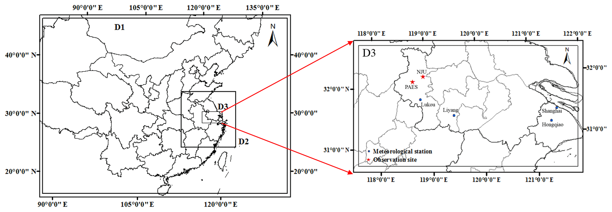
Figure 1Modeling domain and locations of two observation sites and four meteorological stations.
As BC is not one of the six regulated air pollutants in the NAAQS, it was a big challenge to obtain observation data with high temporal resolution in most cities of southern Jiangsu. For the whole year 2015, hourly ambient BC concentrations were available at two sites in Nanjing, the capital of Jiangsu. As illustrated in Fig. 1, one is a suburban site located in the Xianlin Campus of Nanjing University in northeast Nanjing (NJU), and the other is an urban site in Jiangsu Provincial Academy of Environmental Science (PAES). At both sites, BC was sampled and analyzed hourly with semi-continuous carbon analyzer (Model-4, Sunset Lab, USA). Details of the measurement approach were described in Chen et al. (2017). The statistics of observed ambient BC concentrations at the two sites are shown in Fig. S2. The annual average BC concentrations (calculated as the mean of January, April, July and October) were 3.83 and 2.47 µg m−3 at NJU and PAES, respectively. The hourly average BC observations ranged 0.06–17.65 µg m−3 and 0.22–19.76 µg m−3 at NJU and PAES, respectively. The values were similar to those observed in the Guanzhong basin (0.4–23.1µg m−3), the Pearl River Delta region (1–13 µg m−3) and the Beijing-Tianjin-Hebei region (2–32 µg m−3) (Li et al., 2016). Much higher BC concentrations were observed in autumn and winter at both sites, with the monthly means at 3.96 and 5.44 µg m−3 at NJU and 3.62 and 2.80 µg m−3 at PAES, respectively.
The scaling factors derived from Eq. (1) were used to constrain BC emissions in southern Jiangsu in JS-prior from a top-down perspective by assuming a near-linear relation between changes in BC concentrations and emissions:
where EJS-posterior is the vector of the total BC emissions from the top-down approach; Epower, Eindustry, Eresidential, and Etransportation are the vectors of BC emissions from power generation, industry, residential sources, and transportation, respectively, in JS-prior.
2.3 Air quality simulation
We used the Models-3 Community Multi-scale Air Quality (CMAQ) version 4.7.1 to simulate ambient BC concentrations. As shown in Fig. 1, three nested domains were applied with horizontal resolutions of 27, 9, and 3 km, respectively, on a Lambert Conformal Conic projection centered at (110∘ E, 34∘ N). The mother domain (D1, 177×127 cells) covered most parts of China and other surrounding countries. The second domain (D2, 118×121 cells) covered Jiangsu, Anhui, Zhejiang, Shanghai, and parts of other provinces in China. The third domain (D3, 133×73 cells) covered Shanghai, part of Anhui province and the city cluster in southern Jiangsu. There were 27 vertical levels from the ground surface up to 50 hPa on terrain-following coordinate. The simulations were conducted for January, April, July and October to represent four typical seasons in 2015. A 5-day spin-up period of each month was applied to minimize the influence of initial conditions in the simulations.
Meteorological fields were simulated by the Weather Research and Forecasting Model (WRF) version 3.4. The ACM2 planetary boundary layer (PBL) mixing scheme, the carbon bond gas-phase mechanism (CB05), and the AERO5 aerosol module were adopted in the WRF/CMAQ model. Relevant details of model configuration can be found in Zhou et al. (2017). Statistical indicators, including averages of simulations and observations, bias, normalized mean bias (NMB), normalized mean error (NME), root mean squared error (RMSE), and index of agreement (IOA) were applied to evaluate the modeling performance of WRF (Baker et al., 2004; Zhang et al., 2006). Ground observation data at 1 or 3 h intervals at meteorological stations, including Lukou, Hongqiao, and Liyang stations in the third domain (labeled in Fig. 1), were taken from the National Climatic Data Center (NCDC). The statistical indicators for temperature at 2 m (T2) and relative humidity at 2 m (RH2), and wind speed and direction at 10 m (WS10 and WD10) for the 4 typical months in 2015 are summarized in Table S4. Discrepancies between ground observations and WRF modeling were within an acceptable range (Emery et al., 2001).
To make it applicable in our CTM, MEIC-prior was downscaled into grid systems of each modeling domain based on the spatial distributions of gross domestic product (GDP, for power generation and industrial emissions) and population (for residential and transportation emissions) at a horizontal resolution of 1 km×1 km. The downscaled MEIC-prior was used for the first and second domains and the regions outside Jiangsu of the third domain, while JS-prior was applied for the Jiangsu region of the third domain. A brute-force method was applied to estimate contributions to ambient BC concentrations by sector. Five scenarios were designed in this study: Scenario B (the base scenario) in which emissions from all sources in the third domain were included, and Scenarios S1, S2, S3, and S4 in which BC emissions from power generation, industry, residential sources, and transportation in the whole third domain were zeroed out, respectively. We compared simulated BC concentrations in S1, S2, S3, and S4 with those in Scenario B in 4 months at two sites, and the contributions from four major emission sectors to ambient BC levels were determined as the differences in simulated concentrations between Scenarios B and S1–S4.
3.1 Bottom-up emission estimate
The total annual BC emissions of JS-prior were estimated at 26.99 Gg for the southern Jiangsu city cluster in 2015, including 0.18 Gg from power generation, 17.67 Gg from industry, 3.80 Gg from residential sources, and 5.33 Gg from transportation, as shown in Fig. 2. Accounting for 66 % of total annual emissions, industry was identified as the dominant contributor to BC, followed by transportation (20 %) and residential sources (14 %). Although the policies of energy conservation and emission control have been conducted for years, there were still a number of small facilities with low operation temperatures and combustion efficiencies in southern Jiangsu, leading to a large amount of BC from incomplete combustion. When scaling emissions from 2012 to 2015, in addition, improvements in emission controls were not taken into account, such as elevated combustion technologies and enhanced use of dust collectors. The potential reductions in net emission factors for major factories, therefore, were not well quantified, and the emissions from industry could be overestimated. Emissions from power generation were few, resulting from the relatively high combustion efficiency of pulverized boilers and large penetrations and removal rates of dust collectors. Besides the annual total, the emissions of 4 months (January, April, July, and October) were also estimated and limited seasonal differences were found as shown in Fig. 2.

Figure 2The monthly (left axis) and annual (right axis) emissions by sector for southern Jiangsu 2015 in JS-prior and JS-posterior (unit: Gg).
Figure S3 shows the spatial distribution of annual BC emissions in JS-prior. For the power generation and industry sectors, the latitude and longitude of each plant were applied to allocate BC emissions, and the outstandingly high emissions shown in the map indicated the existence of big power and industrial plants. For residential sources, large emissions were found in the regions with intensive population. Emissions from transportation were mainly distributed along the road net and downtown regions in southern Jiangsu cities (see the geographic locations of downtowns in Fig. S1), slightly overlapping with those from residential sources.
3.2 Top-down emission estimate
The time series of BC concentrations contributed by various sectors (c in Eq. 1) were simulated with CTM and illustrated in Figs. S4 and S5 for NJU and PAES, respectively. Among all the sectors, the largest seasonal variation in BC contribution was found for residential sources. The average concentrations contributed by this sector in January reached 0.76 and 0.94 µg m−3 at NJU and PAES, respectively, approximately twice those in another 3 months. The concentrations contributed by industry were significantly enhanced in certain periods (e.g., 20 January, 9–11 April, and 15–17 July), and industrial emissions were expected to be an important reason for the overestimation in BC concentrations through CTMs (see the model evaluation in Sect. 3.3). Table S5 summarizes the monthly and annual mean BC contributions by sector. The annual contributions of industry at the two sites were close to each other (21.0 % and 21.9 % at NJU and PAES, respectively). Contributions of residential sources and transportation were higher at PAES, resulting from a large population and heavy traffic in the urban area. A minor contribution of power generation to BC concentrations was found at both sites (the annual means were less than 1 %), attributed to its very limited emissions. The total contributions from the four sectors were larger than 50 % for all the months and sites except for January. We assumed that the smaller contributions in January resulted partly from the longer lifetime of BC due to less wet deposition in winter. Moreover, we conducted the cluster analysis of back trajectories of air masses arriving at NJU with the Hybrid Single Particle Lagrangian Integrated Trajectory (HYSPLIT, version 4) model, and found that fewer air masses passed through the third modeling domain in January, as illustrated in Fig. S6. The result thus implied more contribution from regional transport to the air quality at the site in winter compared to other seasons. We acknowledged that the multiple regression model was less effective in identifying the sources of BC in winter by constraining the emissions in the southern Jiangsu city cluster alone.
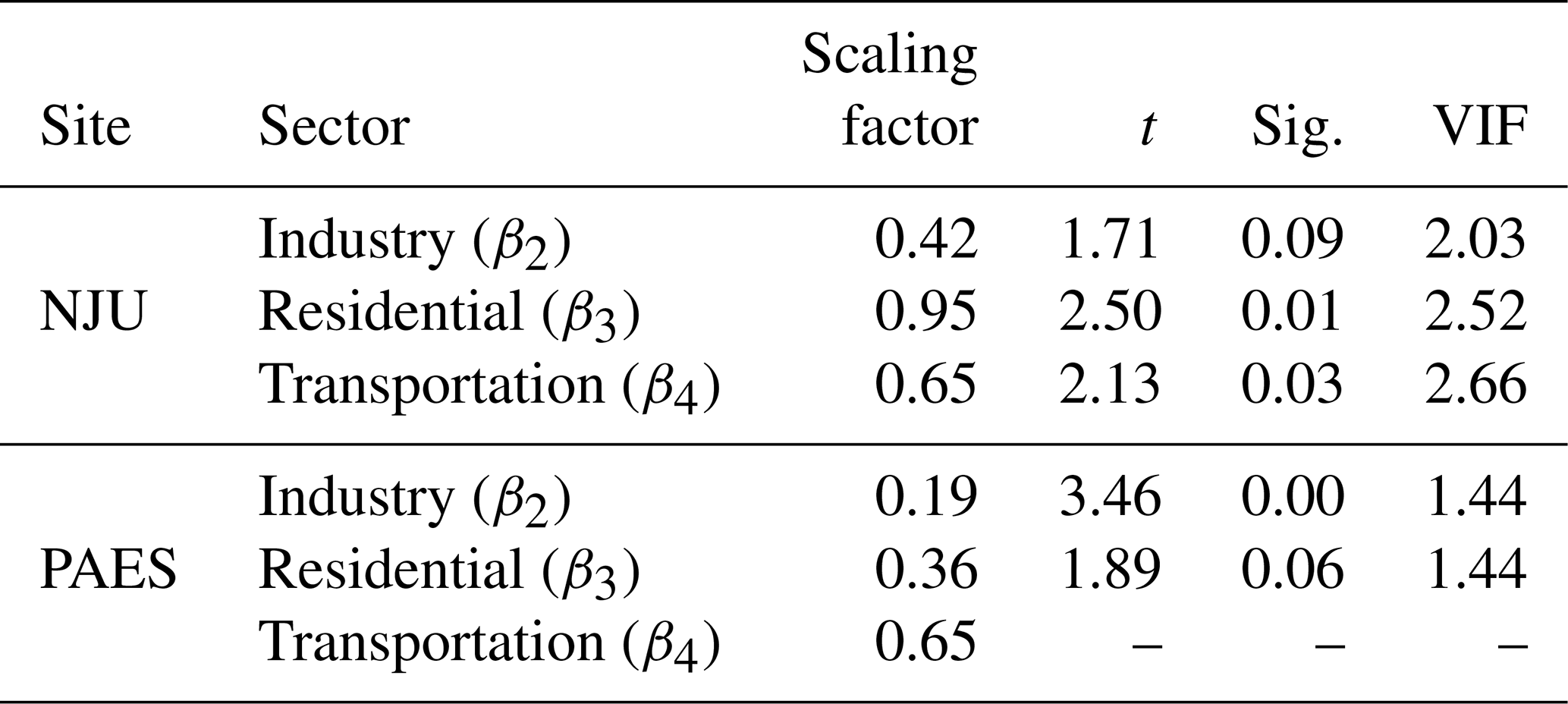
Table 1The scaling factors and statistical indicators from the multiple regression model for estimation of JS-posterior.
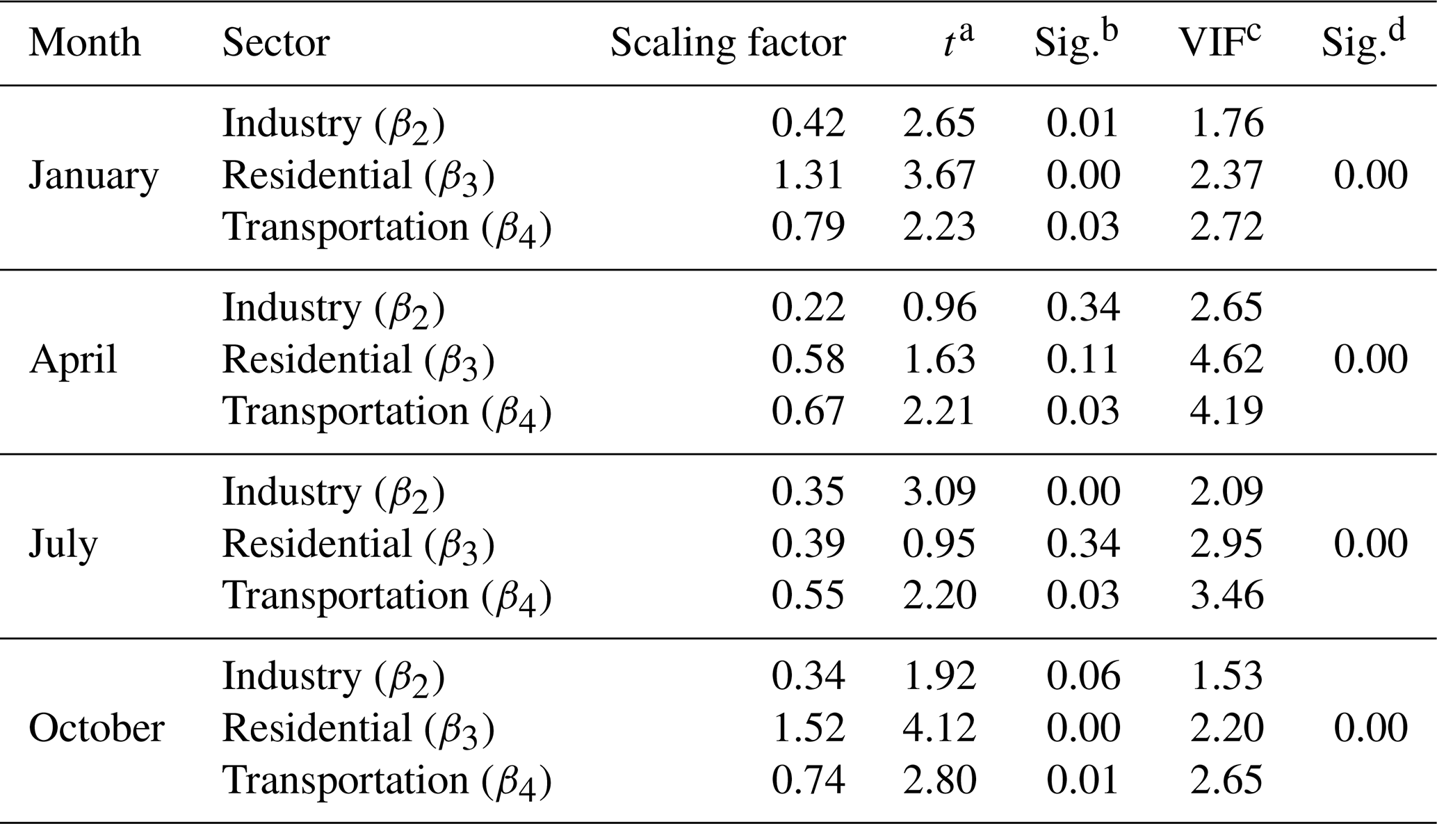
Note: the criteria for the statistical significance of the model: a t>2, b Sig. < 0.05, and c VIF < 10, and d the overall significance < 0.05.
Summarized in Table 1 are the scaling factors β1–β4 estimated from the multiple regression model (Eq. 1) by season, together with the statistical indicators, including the values of t, Sig. (or p), and the variance inflation factor (VIF). The values of t and Sig. indicate statistical significance with thresholds of 2 and 0.05, respectively. The VIF is a test for multicollinearity and the model is reasonable when VIF values in the table are much smaller than 10. Since the emissions from power generation were small and they contributed very little to ambient BC concentrations, inclusion of the power generation component would not significantly improve the regression model. In this study, therefore, we assumed that the simulated BC concentrations from power generation were correct by setting β1 at 1, and we further subtracted them from the observations. Most statistical indicators in Table 1 met the criteria (t>2, Sig. < 0.05, VIF < 10) and the overall significance was 0.00 in 4 months, implying acceptable robustness of the multiple regression model. However, the results were not statistically significant, indicated by t and Sig. values for some months and sectors (e.g., industry in April and October and residential in April and July), implying that the constrained emissions for those months/sectors need to be cautiously analyzed.
By applying β1–β4 in Eq. (2), the top-down estimates of BC emissions (JS-posterior) were estimated and illustrated in Fig. 2. The total BC emissions for the southern Jiangsu city cluster were calculated at 13.4 Gg, 50 % smaller than those of JS-prior. For the capital city of Jiangsu province, Nanjing, Huang et al. (2019) conducted a detailed analysis of the changes in operation activities and emission control technologies of individual sources based on annually updated official environmental statistics and pollution census. With the bottom-up approach, the annual BC emissions in the city were estimated to decrease by 60 % from 2012 to 2015 as shown in Fig. S7. The relative change in annual emissions (60 %) was close to that between JS-prior and JS-posterior (50 %), implying the constraining approach in this work could capture the changes in emissions due to improved control measures.
The scaling factors of emissions from industry and transportation (β2 and β4) ranged from 0.22 to 0.42 and from 0.55 to 0.79 for different months, respectively. Accordingly, the emissions from industry and transportation in JS-posterior were estimated to be 67 % and 32 % smaller than those in JS-prior, respectively. As mentioned above, the emissions in JS-prior in 2015 were simply scaled from those in 2012 according to activity data, and changes in emission factors were not considered. In actual fact, however, a series of measures in industry and transportation were conducted to improve energy efficiency and to reduce emissions over recent years. Issued in 2013, for example, the Air Pollution Control Planning for the Key Regions for the 12th Five-Year Plan period (2010–2015) aimed to achieve 7 % and 15 % reductions in the annual average concentration and industrial emissions of fine particles in Jiangsu province from 2010 to 2015, respectively (Qian, 2013). The measures included eliminating old and energy-inefficient plants of heavy-polluted industries (thermal power generation and steel/building material production), and optimizing the energy structure through application of sustainable energy. Meanwhile, the enhanced use of cleaner gasoline and diesel products (National Standard Stage V) in transportation could lead to reduced vehicle emissions. The government efforts in emission controls proved effective, indicated by the scaling factors much smaller than 1 (β2 and β4 in Table 1) and the reduced emissions of JS-posterior. For residential sources, the emissions in JS-posterior were 3 % smaller than those in JS-prior, indicating a limited difference in the annual total emissions between the two inventories. However, the scaling factors (β3) in January and October were 1.31 and 1.52, respectively, showing a stronger enhancement in BC emissions in winter and autumn in JS-posterior than those in JS-prior. It thus implied that there were missing sources likely associated with low-quality fossil fuels or biofuel used for heating in winter and crop waste burning in autumn in JS-prior.
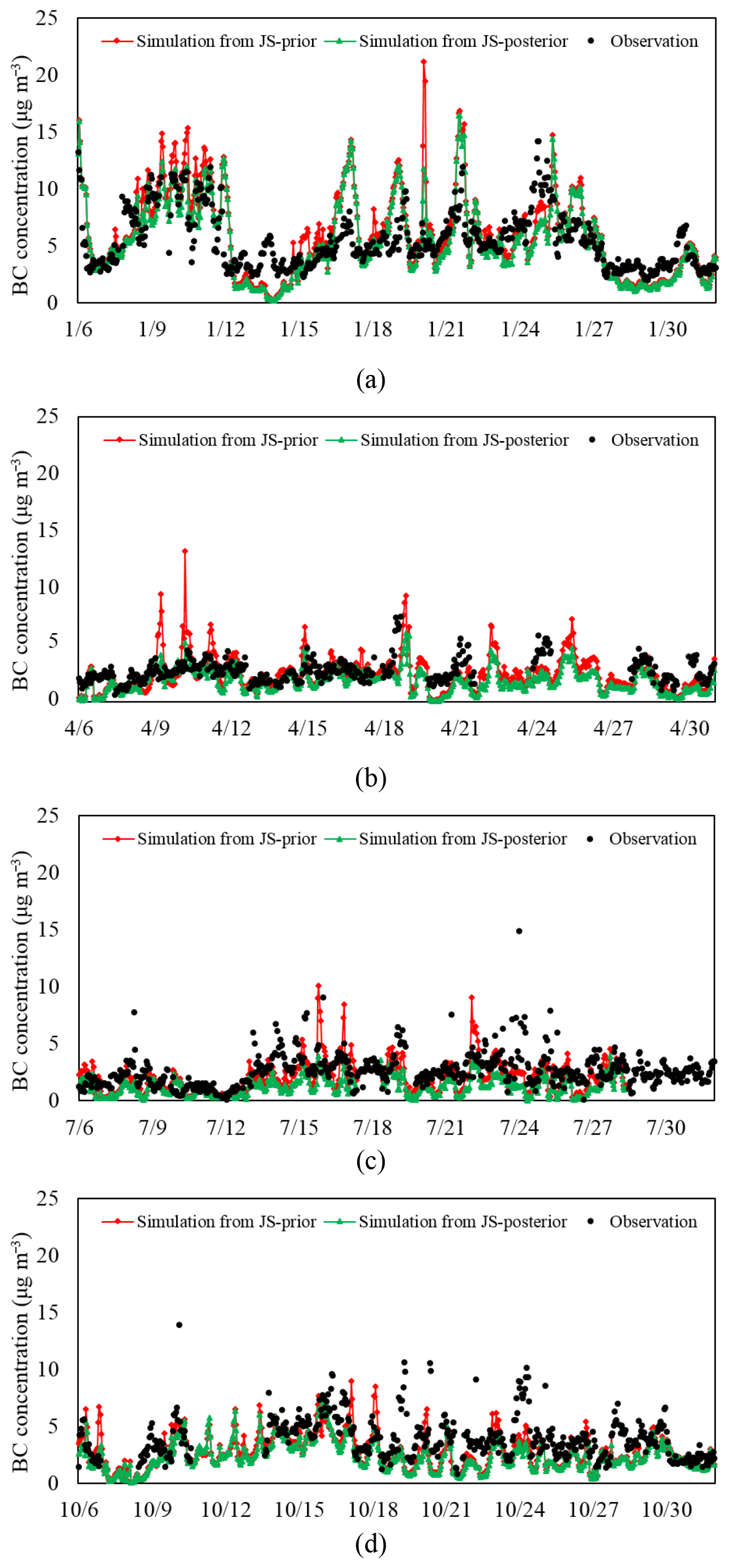
Figure 3The observed and simulated hourly BC concentrations at NJU using JS-prior and JS-posterior for January (a), April (b), July (c), and October (d) in 2015 (unit: µg m−3).
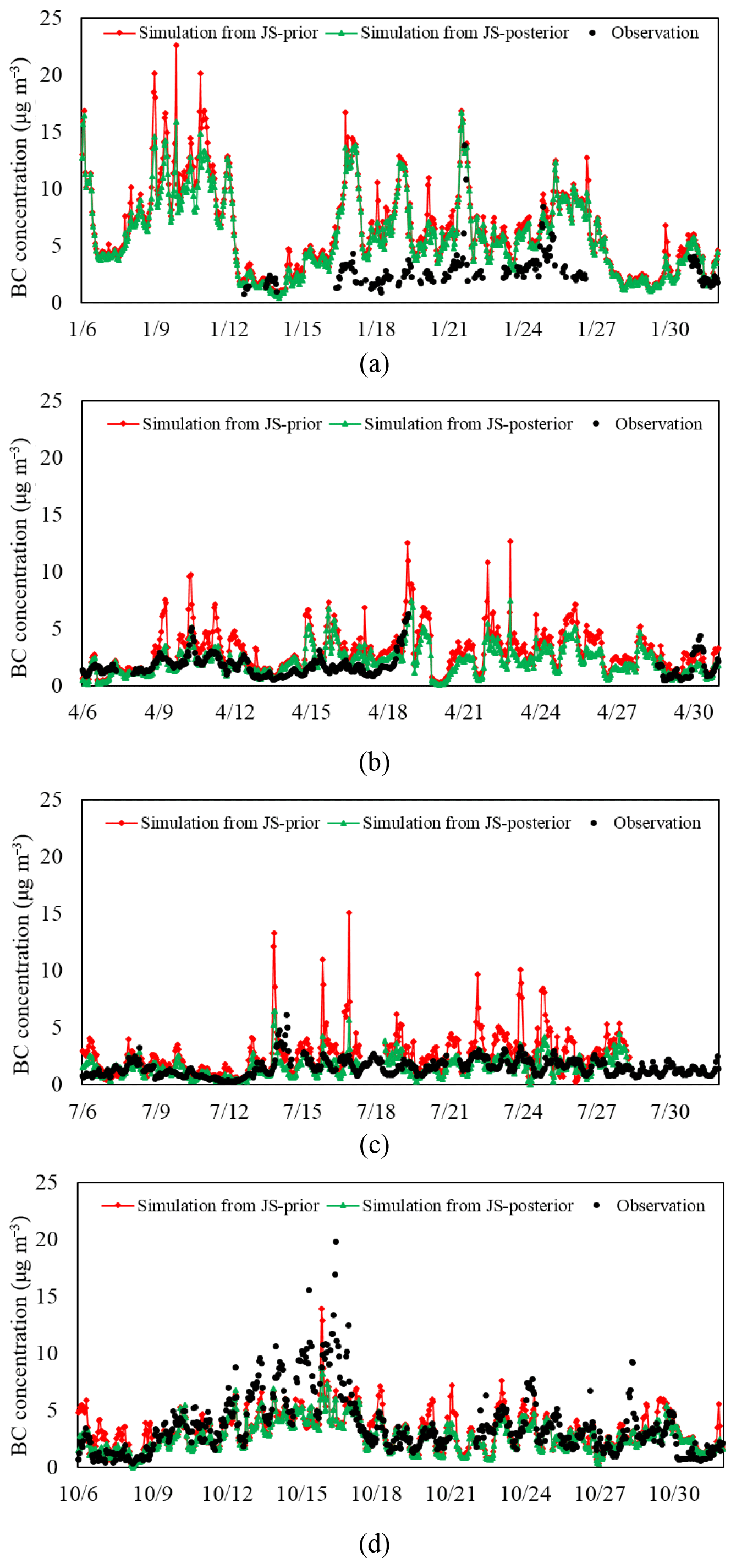
Figure S8 presents the seasonal variations in BC emissions of JS-prior, JS-posterior, and MEIC-prior by sector, and stronger variations were generally found in JS-posterior. As shown in Fig. S8a, the largest difference among the three inventories existed in the residential sources, and the ratio of maximum to minimum monthly emissions was 4.33 in JS-posterior, close to that in MEIC-prior at 4.00 and nearly 4 times that in JS-prior at 1.13. The ratios of maximum to minimum monthly emissions were 1.13, 1.83, and 1.29 for JS-prior, JS-posterior, and MEIC-prior, respectively (Fig. S8b). The value for JS-posterior was closer to 2.1 for an anthropogenic BC emission inventory in China by Lu et al. (2011) that considered enhanced use of fossil fuels for residential heating in winter in northern China. The comparison thus implied again that current bottom-up inventories might underestimate the emissions of residential solid fuel burning in winter in southern Jiangsu. As central household heating was not conducted in the area in winter, the official energy statistics on which bottom-up inventories were based may not fully capture the elevated fuel burning by disperse households. Spatial distribution of BC emissions in JS-posterior was illustrated in Fig. S3. Compared to JS-prior, BC emissions from industry and transportation were greatly reduced in downtown regions in the southern Jiangsu city cluster.
3.3 Evaluation of the top-down emission estimate
The simulated BC concentrations based on bottom-up (JS-prior) and top-down estimation in emissions (JS-posterior) were compared with observations to evaluate the two inventories, and the results were illustrated in Figs. 3 and 4 for NJU and PAES, respectively. Statistical indicators including mean concentrations from simulations and observations, NMB and NME, as well as the regression correlation (R) were calculated to evaluate the modeling performance, as summarized in Table 2.
Table 2Statistical indicators for observed and simulated BC concentrations using JS-prior and JS-posterior at NJU and PAES.
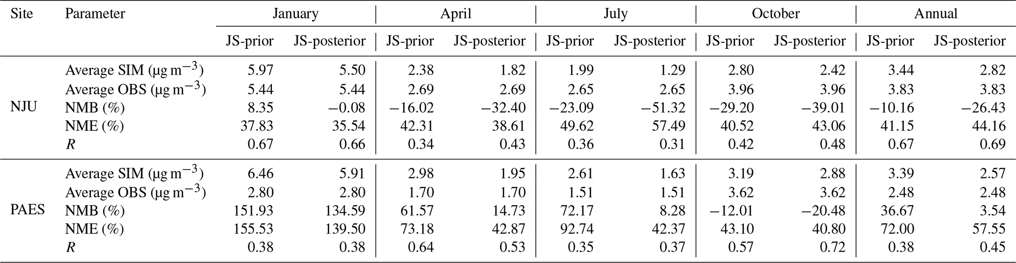
Note: SIM and OBS indicated the results from simulation and observation, respectively. NMB and NME were calculated using following equations (P and O indicated the results from modeling prediction and observation, respectively): ; .
In general, CTM based on JS-prior reproduced well the temporal variations of the observed BC concentrations at the two sites. The highest and lowest concentrations were, respectively, simulated in winter and summer, consistent with observations with an exception at PAES where the observed monthly mean in January (2.80 µg m−3) was lower than that in October (3.62 µg m−3). The overestimation in January at PAES (especially in middle and late 16–26 January) might result partly from the emission control policy implemented for the National Memorial Day of Nanjing Massacre Victims on 13 December 2014. During the period, Nanjing undertook a series of stringent restrictions on air pollutant emissions. For example, key petrochemical and steel industries were shut down, and all the high-pollution vehicles were forbidden from driving into the city. Those restrictions had large impacts on emissions and thereby air quality in the following month at PAES, but were not fully considered in current emission inventories. Moreover, the bias could be enhanced under certain meteorology conditions. As illustrated in Fig. S9, higher daily average PBL height at PAES was found for periods when the simulated concentrations were relatively lower (e.g., 6–7, 12–15, and 28–31 January), resulting in smaller bias between simulation and observation. In contrast, the lower PBL height found in other periods would exaggerate the overestimation in simulated concentrations, given the elevated emissions in JS-prior. The seasonal variation of BC concentrations at NJU was larger than that at PAES, suggesting a bigger impact of household solid fuel use on the suburban and rural regions. Though the model was able to capture the seasonal variability, discrepancies between simulations and observations existed, and CTM generally underestimated BC concentrations at suburban site NJU and overestimated those at urban site PAES. With the monthly means ranging from 1.99 to 5.97 µg m−3 at NJU, the annual average BC concentration (calculated as the mean of January, April, July, and October) was simulated at 3.44 µg m−3, smaller than the observed 3.83 µg m−3. With the monthly means ranging from 2.61 to 6.46 µg m−3, in contrast, the annual concentration at PAES was simulated at 3.39 µg m−3, larger than the observed 2.48 µg m−3. Better correlation between observation and simulation was found at NJU, indicated by the larger R. The annual mean NMBs were calculated at −10.16 % and 36.67 %, and the NMEs were 41.15 % and 72.00 % at NJU and PAES, respectively. The discrepancy suggested that JS-prior used in CTM might misrepresent the spatial pattern of emissions. Population and economy densities were applied to allocate BC emissions, leading to overestimation in emissions and thereby simulated concentrations in urban areas with more population and economic activity. Besides, the model overestimated the peak surface concentrations at both sites particularly when the contribution from the industry sector was enhanced as mentioned in Sect. 3.2 (e.g., 9–11 January and 9–10 April at NJU, and 9–12 April, the second half of July, and 20 October at PAES).
Application of JS-posterior in CTM effectively corrected large biases between simulations and observations at the two sites. As shown in Table 2, NMEs were reduced for most months (all months at PAES and January and April at NJU) while effects of applying JS-posterior in CTM varied at two sites. At PAES, the annual average NME declined from 72.00 % to 57.55 % and the annual mean of BC concentration was simulated at 2.57 µg m−3, in better agreement with the observed 2.48 µg m−3 than the simulated 3.39 µg m−3 using JS-prior. The largest reductions in NMEs were found in April and July, from 73.18 % to 42.87 % and from 92.74 % to 42.37 %, respectively. Moreover the overestimations in peak concentrations using JS-prior were partly corrected when JS-posterior was applied, resulting mainly from the reduced emissions from industry and transportation. Regarding the overestimation in 16–26 January discussed above, we excluded the data points for those dates and re-compared the observation and simulation. As can be seen in Table S6, the overestimation in CTM was largely reduced and the top-down estimate corrected the bias moderately in January at PAES. Besides the emissions, overestimation in annual BC concentration at PAES could result partly from the uncertainty in PBL modeling (Liu et al., 2018). As shown in Table S7, the monthly PBL heights in WRF were generally lower than those in actual atmosphere, leading to enhanced BC concentrations.
Although simulations of peak concentrations at NJU were improved as well, the annual average NME at NJU slightly increased from 41.15 % to 44.16 % and the annual mean of BC concentration was simulated at 2.82 µg m−3, smaller than the simulated 3.44 µg m−3 using JS-prior. Bigger bias was found in July and October at NJU, since the reduced emission estimates in JS-posterior led to further underestimation in simulated ambient BC levels compared to JS-prior. Limitation of the current multiple regression model thus indicated that overestimation and underestimation in concentrations at different sites could hardly be corrected simultaneously without further improvement in spatial distribution of emissions.
We selected April to evaluate the sensitivity of observation and bottom-up emission input to top-down constraint. Observation site number, spatial representativeness of sites, and the a priori bottom-up inventory were changed separately in the constraining approach, and various top-down estimates could be derived and compared with each other. Furthermore, we evaluated the uncertainty of the multiple regression model, including the assumption of near linearity between emissions and concentrations in July and October and the impact of precipitation in July. The statistical indicators of modeling performances based on different cases are summarized in Table 3. Details were described as below.
Table 3Statistical indicators for observed and simulated BC concentrations in different cases at NJU and PAES (Cases 1–5 for April and Cases 6–7 for July).
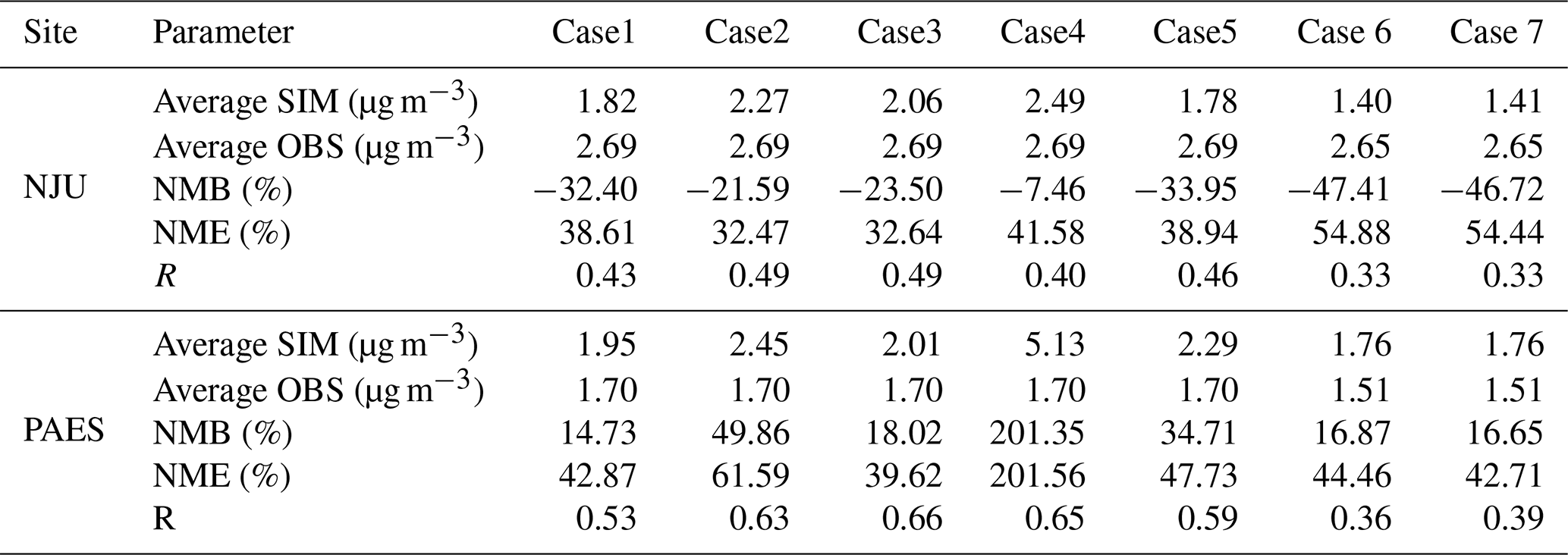
Note: Case 1 applied observations at two sites to constrain the emissions from the whole city cluster (JS-posterior); Case 2 applied observations at only one site (NJU) to constrain the whole city cluster; Case 3 applied observations at two sites to constrain emissions from different cities, respectively; Case 4 applied MEIC-prior; Case 5 applied MEIC-posterior; Case 6 excluded the data influenced by simulated wet deposition; and Case 7 excluded the data influenced by satellite-derived accumulative precipitation.
4.1 The effect of observation data application
A major challenge in understanding the sources and distributions of BC in China was the lack of a consistent and stable measurement network with good spatiotemporal coverage, such as the IMPROVE network in the United States (Malm et al., 1994). Uncertainty existed in the top-down estimates in this work, as hourly measurements of BC concentrations were only available at two sites in southern Jiangsu. Therefore, besides JS-posterior derived from observations at both sites in April as described in Sect. 3.2 (mentioned as Case 1 hereinafter), we conducted a Case 2 in which observation data at only one site (NJU) were used in the top-down approach, to analyze the effect of the site number on emission estimates.
The scaling factors of emissions from industry, residential sources and transportation were recalculated at 0.42, 0.95 and 0.65, respectively. Compared to JS-prior in April in Table 2, the NMEs of Case 2 in Table 3 decreased from 42.31 % to 32.47 % and from 73.18 % to 61.59 % at NJU and PAES, respectively, implying the benefits of ground measurements (even available only at one site) on emission constraint. The NME in Case 2 was slightly smaller than that in Case 1 at NJU, suggesting that application of measurement data at one single site could improve modeling performance moderately at that site. At PAES, in contrast, much larger NME was found in Case 2. Much better modeling performance in Case 1 at PAES indicated that inclusion of more measurements with better spatiotemporal coverage could constrain BC emissions at the city cluster level more effectively. It should be noted that the number of data included in the multiple regression model was 48 % of those for the whole period with the data screening mentioned in Sect. 2.2. In particular, the period lack of observation accounted for 38 % of the whole month. We further analyzed the CTM performances for the periods included in the model and those excluded from the model separately, as shown in Table S8. The observed concentration for the periods included in the model (2.56 µg m−3) was smaller than the simulated in JS-prior (2.71 µg m−3), leading to the reduced emissions through constraining. The constrained emissions resulted in a simulated concentration (2.42 µg m−3) closer to the observation for the periods included in the multiple regression model, and did not increase the bias for the periods excluded from the model. It suggested that factors other than emissions in CTM (e.g., meteorology) might contribute to the underestimation for the latter.
Besides the number of observation sites, spatial representativeness was also identified and its impact on top-down emission constraint was evaluated. Considering the prevailing winds from northeast and southeast, on the one hand, NJU located upwind of Nanjing is hardly influenced by the emissions from the downtown of the city. Besides, the site is downwind of the YRD, including the Suzhou–Wuxi–Changzhou–Zhenjiang city cluster (Chen et al., 2017), and thus it is more representative of the western YRD emissions through regional transport. On the other hand, PAES is located in urban Nanjing and its air quality is commonly influenced by surrounding transportation, residential, and commercial sources; thus, the site is representative of the local emissions of Nanjing. In contrast to previous top-down studies that did not distinguish the influence of local emissions and transport on air quality in sub-regions of the research domain (Wang et al., 2011; Fu et al., 2012), the spatial representativeness of the two observation sites were taken into account to improve the top-down approach and the result of constraining BC emissions in the southern Jiangsu city cluster. Through the brute-force method described in Sect. 2.3, we zeroed out the emissions from Nanjing and the Suzhou–Wuxi–Changzhou–Zhenjiang city cluster in CTM, respectively, and compared the simulated concentrations with those in Scenario B to analyze the contributions of the two regions to ambient BC concentrations at NJU and PAES. As shown in Fig. S10, the contribution of emissions from Nanjing to PAES was greater than that to NJU in 82 % of the modeling period, and the analog number was 81 % for the contribution of the Suzhou–Wuxi–Changzhou–Zhenjiang city cluster to NJU greater than that to PAES. We thus concluded that emissions from Nanjing contributed significantly to PAES, while those from the Suzhou–Wuxi–Changzhou–Zhenjiang city cluster contributed significantly to NJU. We then developed a new case of top-down emission estimate in southern Jiangsu (Case 3), in which observation data at PAES and NJU were applied to constrain emissions from Nanjing and the Suzhou–Wuxi–Changzhou–Zhenjiang city cluster, respectively.
Table 4The scaling factors and statistical indicators from the multiple regression model in Case 3.
The scaling factors in Case 3 are provided in Table 4. To avoid the collinearity in the multiple regression model, we expected that the relative changes in emissions from transportation in Nanjing and the Suzhou–Wuxi–Changzhou–Zhenjiang city cluster were similar for recent years, resulting from the same progress of emission standard implementation (National Standard Stage IV) in southern Jiangsu and the frequent circulation of vehicles among the cities. Therefore the same scaling factor was assumed for transportation in the two regions. As shown in Table 4, all the scaling factors at PAES were smaller than those at NJU, implying that implementation of emission controls in Nanjing was more stringent than that in the Suzhou–Wuxi–Changzhou–Zhenjiang city cluster from 2012 to 2015. As the host city of the 2nd Asian Youth Games in 2013 and the 2nd Youth Olympic Games in 2014, Nanjing undertook a series of restrictions on air pollutant emissions. The city had conducted emission control action on small coal-fired boilers since 2013 and over 1200 coal-fired boilers had been shut down by the end of 2014. In addition, central heating units were largely applied to replace the coal with electricity, natural gas, or biofuel. As shown in Table 3, the NMEs in Case 3 were the smallest at both sites among all the cases, with an exception: the NME at NJU in Case 3 was 32.64 %, slightly larger than that in Case 2 at 32.47 %. The result implied that inclusion of more measurement data with their spatial representativeness considered could improve the top-down approach in terms of spatial distribution of emissions and could reduce the deviation between observations and simulations.
Summarized in Table S9 are BC emissions from Nanjing and the Suzhou–Wuxi–Changzhou–Zhenjiang city cluster estimated in different cases. All the top-down estimates were approximately half of the bottom-up estimate and the estimate in Case 1 was the smallest among all the cases. The same scaling factors were generated and applied in Cases 2 and 3 to calculate BC emissions from the Suzhou–Wuxi–Changzhou–Zhenjiang city cluster which accounted for 80 % of the total emissions in southern Jiangsu, resulting in similar top-down emission estimates between the two cases.
4.2 The effect of the a priori bottom-up emission input
Given the large uncertainty in JS-prior that was simply developed based on the changes in activity levels in recent years, we applied MEIC-prior as well to explore the effect of the a priori emission inventory on top-down BC constraints.
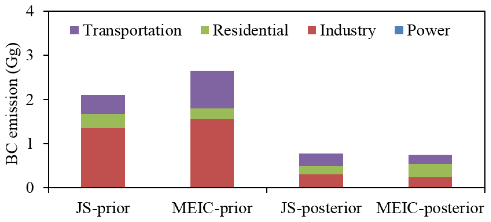
Figure 5BC emission estimates by source of JS-prior, MEIC-prior, JS-posterior, and MEIC-posterior in April 2015 in southern Jiangsu (unit: Gg).
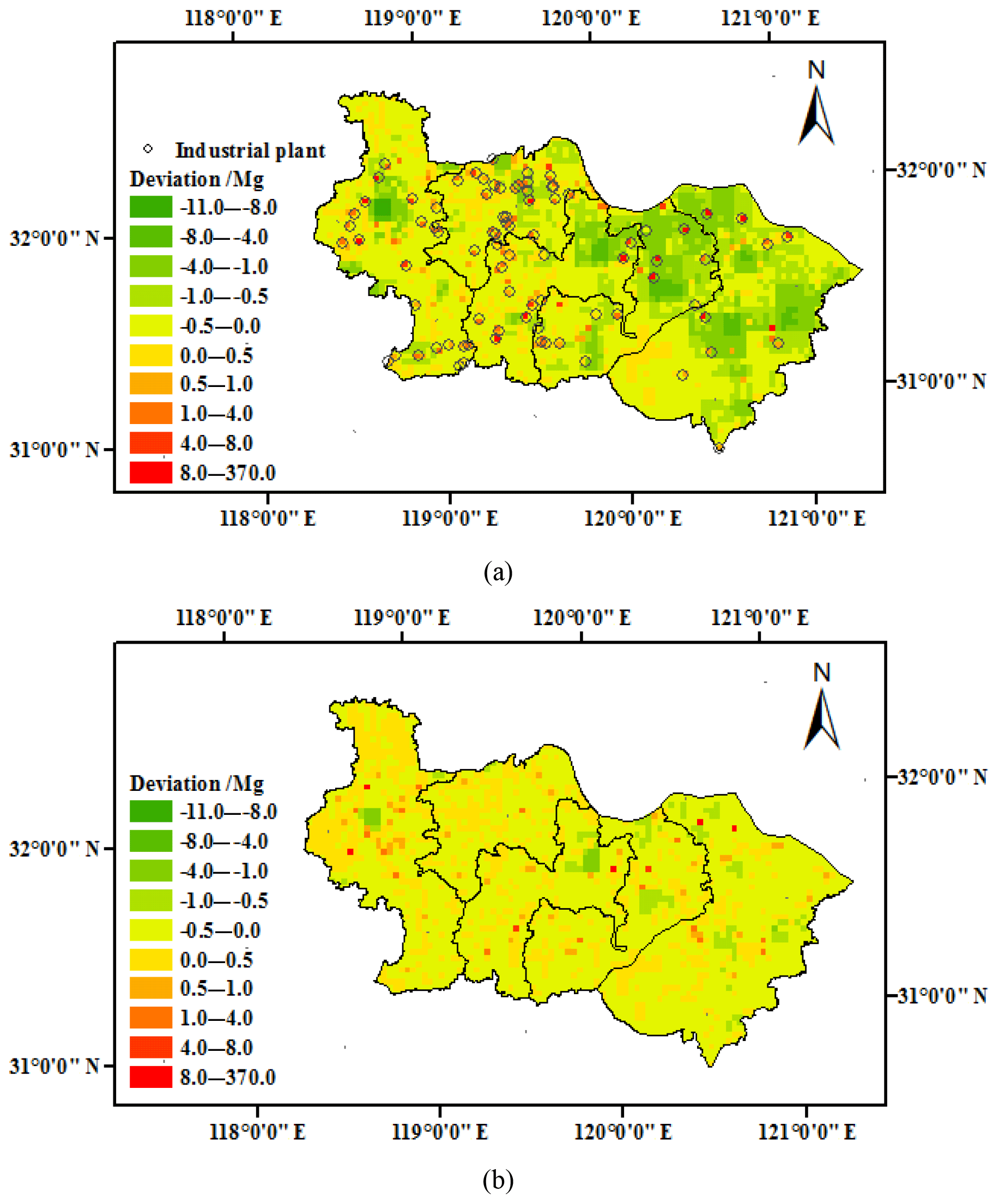
Figure 6The spatial distributions of the deviations (JS-MEIC, unit: Mg) between JS-prior and MEIC-prior (a) and those between JS-posterior and MEIC-posterior (b).
Figures 5 and 6a compare the total amount and spatial distribution of emissions between JS-prior and MEIC-prior in April for southern Jiangsu, respectively. The total BC emissions in JS-prior were 21 % lower than those in MEIC-prior. In JS-prior, as shown in Fig. 6a, the emissions from some industrial plants were extremely larger than those in MEIC-prior, while the emissions in urban areas were found to be smaller. Both inventories indicated extremely small contribution from power generation. BC emissions from the industry sector were calculated at 1.34 Gg in JS-prior, 0.22 Gg smaller than MEIC-prior. Emissions from industry in MEIC-prior were calculated based on the regional average of emission factors and allocated according to the spatial distribution of GDP. The method would possibly result in underestimation in emissions from big industrial plants but overestimation in urban areas. Emissions from residential sources in JS-prior were close to those in MEIC-prior, as a similar methodology was applied for the sector in the two inventories. BC emissions from transportation in MEIC-prior (0.85 Gg) were twice those in JS-prior (0.42 Gg), attributable probably to the application of different emission factors. For on-road transportation, the emission factors in JS-prior were calculated with the CORPERT model (EEA, 2012; Zhou et al., 2017), while they were obtained from available domestic measurements in MEIC-prior.
Simulation Case 4 was determined using MEIC-prior in CTM. Following the top-down approach described in Sect. 2.2, we developed Case 5, using MEIC-prior instead of JS-prior as the a priori input of emission data in CTM. The scaling factors of emissions from industry, residential sources, and transportation were, respectively, calculated at 0.15, 1.30, and 0.25 through the multiple regression model, and the top-down estimates in BC emissions (mentioned as MEIC-posterior hereafter) were calculated at 0.75 Gg in April 2015, close to 0.78 Gg in JS-posterior (Fig. 5). The differences in the emissions from industry and transportation between JS-posterior and MEIC-posterior were 0.06 and 0.07 Gg, respectively, much smaller than those between JS-prior and MEIC-prior. Besides the total amount, differences in spatial distribution in industry plants and urban areas between the top-down estimates (JS-posterior and MEIC-posterior) were also significantly reduced compared to those between bottom-up estimates (JS-prior and MEIC-prior), as shown in Fig. 6b.
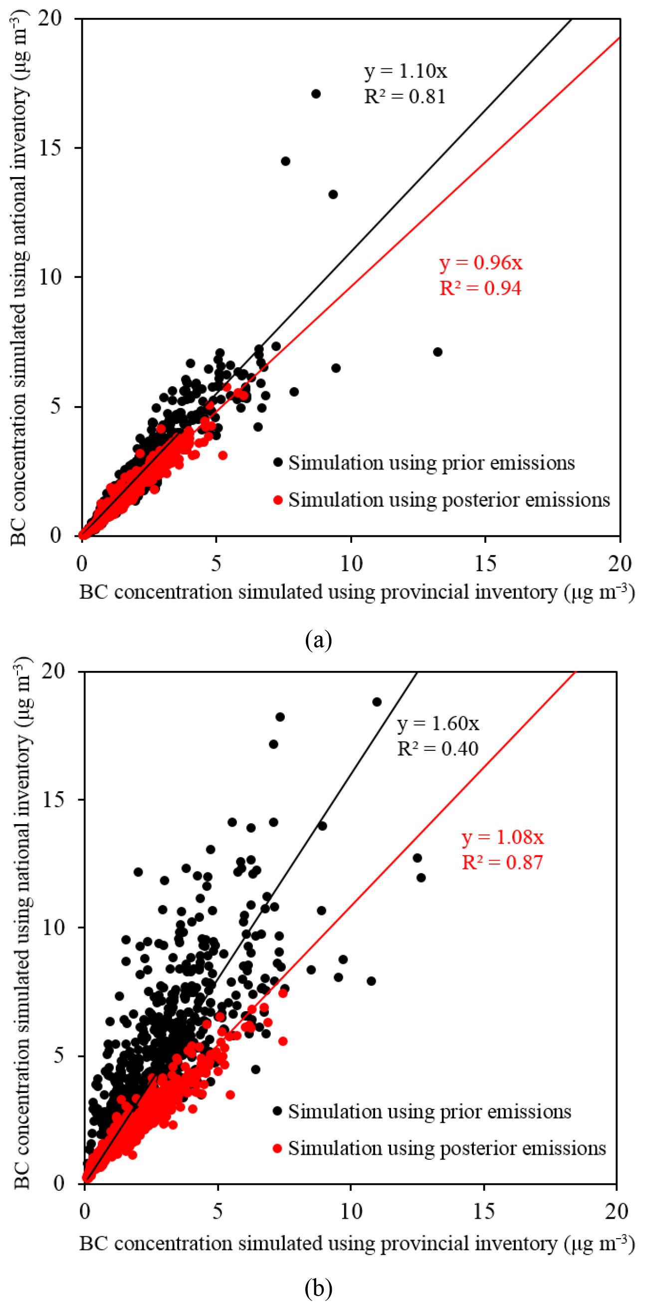
Figure 7The scatter plots of the simulated BC concentrations using JS inventories vs. those using MEIC at NJU (a) and PAES (b).
As shown in Table 3, the monthly average BC concentration at NJU in Case 4 was simulated at 2.49 µg m−3 for April 2015, close to the 2.38 µg m−3 simulated with JS-prior in Table 2. At PAES, however, application of MEIC-prior in CTM resulted in a much larger concentration than JS-prior (5.13 vs. 2.98 µg m−3), indicating again that MEIC-prior would overestimate the emissions in urban areas. Figure 7 illustrates the scatter plots of the simulated BC concentrations from bottom-up and top-down inventories at NJU (Fig. 7a) and PAES (Fig. 7b). Using two bottom-up inventories in CTM, a bigger difference in simulated BC concentrations was found at PAES compared to that at NJU, indicated by the slope (1.10) closer to 1 at NJU in Fig. 7a. The correlation coefficients (R2) between simulated BC concentrations using JS-prior and MEIC-prior were 0.81 at NJU and 0.40 at PAES, respectively. Using two top-down estimates, the difference between simulated concentrations at PAES was significantly reduced and the slope got much closer to 1 in Fig. 7b. The correlation coefficients (R2) were enhanced to 0.94 and 0.87 at NJU and PAES, respectively.
To summarize, similar results from the top-down constraint approach could be obtained in emission level, spatial distribution, and CTM performance; even clear differences existed in the a priori bottom-up inventories. In other words, a limited effect of the a priori emission input was evaluated on the top-down estimate from the multiple regression model.
4.3 Evaluation of the near-linearity assumption in the multiple regression model
As mentioned in Sect. 2.2, the assumption of near linearity between emissions and concentrations is a principle of the multiple regression model, given the weak chemistry reactivity of BC. The principle has been applied in previous studies to constrain BC emissions (Fu et al., 2012; Kondo et al., 2011; Wang et al., 2013; Park et al., 2003; Verma et al., 2017). In actual fact, however, processes other than chemical reaction, e.g., precipitation or wet deposition, impact the linearity. Therefore, the near-linear assumption needs to be justified, and the uncertainty of the methodology could then be evaluated.
Sensitivity analysis was conducted to assess the rationality of the brute-force method described in Sect. 2.3, in which emissions of a given sector were zeroed out to determine their contribution to the ambient concentrations. As summarized in Table S10, we calculated the ratio of simulated wet deposition to emissions by month for NJU, PAES, and the whole southern Jiangsu city cluster with JS-prior and JS-posterior, respectively. July and October were identified as the months with the most and least impact from precipitation, suggested by the largest and smallest ratios, respectively. Two sensitivity simulations were then conducted for the selected 2 months, in which doubled and halved emissions (i.e., 200 % and 50 % of emissions in JS-prior, respectively) were used in CTM, and the simulated concentrations were then compared to those with JS-prior at NJU and PAES, as shown in Figs. S11 and S12, respectively. It suggested that the impact of nonlinearity between emissions and concentrations was limited, no matter whether the precipitation was strong or not. As the top-down constrained emissions (JS-posterior) were 50 % smaller than the bottom-up estimates (JS-prior), the relative change was far beyond the uncertainty from nonlinearity (±10 %, as discussed in Fig. S12), implying the improvement of the top-down approach on emission estimation.
Table 5The scaling factors and statistical indicators from the multiple regression model in Cases 6 and 7.

Table 6The monthly and annual emissions by sector for southern Jiangsu 2015 in Cases 6 and 7 (unit: Gg) and the relative deviation compared to JS-posterior (RD: Case 6 or 7–JS-posterior) ∕ JS-posterior, %).
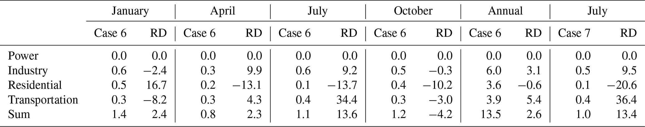
Many studies have reported the difficulty in precipitation simulation with WRF (Annor et al., 2017; Liu et al., 2018; Yu et al., 2011; Yang et al., 2014; Kaewmesri, 2018). In this study, the observed ground precipitation at Lukou, Liyang and Shanghai stations (see Fig. 1 for locations) was compared with the simulated one to evaluate the WRF performance for precipitation modeling. As shown in Figs. S13–S16, the model generally overestimated the amount. Similar results were found in previous studies that WRF overestimated precipitation at fine spatial resolution (Politi et al., 2018; Kotlarski et al., 2014; García-Díez et al., 2015). Improvement in physics parameterization schemes in WRF will help better understand the wet deposition of BC through simulation. To further evaluate the effect of wet deposition on emission constraining, we conducted an extra Case 6, in which the data influenced by simulated wet deposition (i.e., the periods with simulated wet deposition at hourly basis) were excluded in the top-down approach. The new scaling factors – estimated from the multiple regression model were summarized in Table 5. By applying – in Eq. (2), the top-down estimates of annual BC emissions in Case 6 were calculated at 13.7 Gg, and the emissions by sector and month were illustrated in Table 6, together with the relative deviation (RD) compared to emissions in JS-posterior. The relative deviations of monthly total emissions between Case 6 and JS-posterior were less than 5 %, with an exception of July at 14 %, and that for annual total was 2.6 %. Larger relative deviations were found for given sources, e.g., residential in January and transportation in July. The deviations, therefore, were much smaller than that between the emissions in JS-prior and JS-posterior. We consequently applied CTM to evaluate the modeling performance with the emissions in Case 6 for July. Illustrated in Table 3 were the simulated BC concentrations and the statistic indicators obtained through comparisons with observation at the two sites. As suggested by the NME and R values, little improvement on CTM performance was achieved with the emissions in Case 6, compared to those with JS-posterior (Table 2). The impact of simulated wet deposition on the top-down approach was thus expected to be moderate in this work.
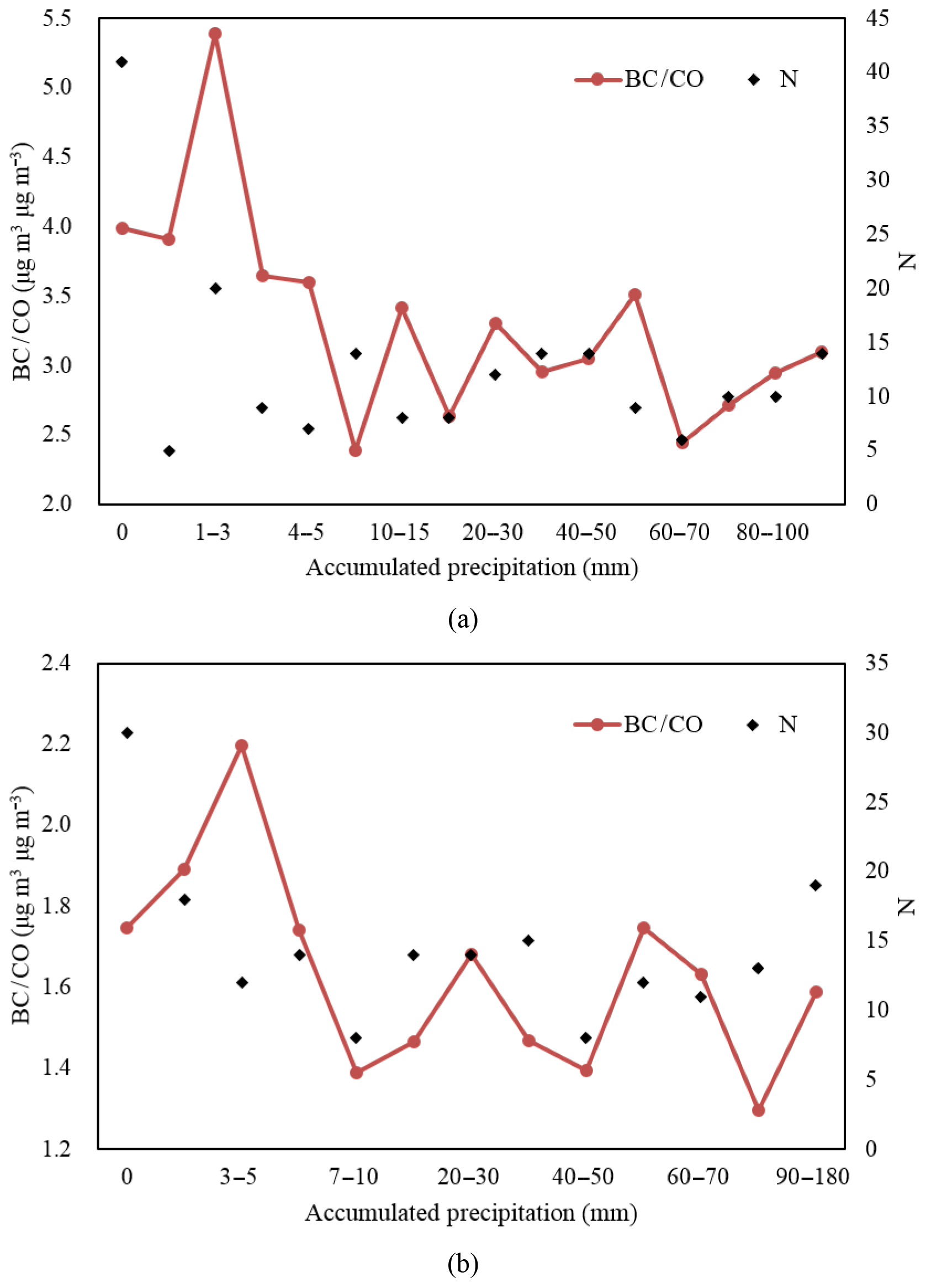
Figure 8The ΔBC∕ΔCO ratio at NJU (a) and PAES (b) separated by different accumulated precipitation along the back trajectories during 48 h. The data point number of each accumulated precipitation interval (right axis) is also given.
As the simulated wet deposition varied from the reality to some extent and the impact of precipitation along the transport was not excluded in Case 6, we selected July to conduct a Case 7, in which the data influenced by accumulative precipitation along the back trajectories at the two sites were excluded in the multiple regression model. The merged high-quality precipitation measured by the Tropical Rainfall Measuring Mission (TRMM) satellite instrument was adopted for wet deposition screening, with a temporal resolution of 3 h and a spatial resolution of . We used the HYSPLIT (version 4.9) model (http://www.ready.noaa.gov, last access: 12 February 2019) to calculate the 48 h back trajectories of the air masses arriving at NJU and PAES. The back trajectories were calculated every 3 h for July with the simulated layer heights of 50, 100, and 500 m above the ground and the time step of 3 h (the same as the temporal resolution of TRMM). The hourly accumulative precipitation along the 48 h back trajectories at two sites was then calculated to determine the BC–CO data pairs influenced by precipitation, given the low effect of precipitation on CO. Figure 8 illustrates the changes in the ΔBC∕ΔCO ratio observed at two sites for different accumulated precipitation intervals. At NJU, the ΔBC∕ΔCO ratio of air masses receiving less than 3 mm accumulated precipitation was significantly larger than that of air masses receiving more than 3 mm, and the analogue number was 5 mm at PAES. In Case 7, therefore, we excluded the BC–CO data pairs receiving more than 3 and 5 mm accumulated precipitation along their trajectories within the last 48 h at NJU and PAES, respectively, in the multiple regression model. It minimized the effect of wet deposition while retaining sufficient data points for the statistical significance. Figure 9 shows the simulated wet deposition in Case 6 and the accumulated precipitation in Case 7 for July to compare the data selection in the two cases. In Case 6, the number of data points were reduced to 65 % of Case 1 after data screening, and over 500 samples at the two sites were available for the multiple regression model. In Case 7, only 31 % of data points remained. The periods excluded in Case 7 contained those in Case 6, implying a stricter data screening to eliminate the effect of precipitation.
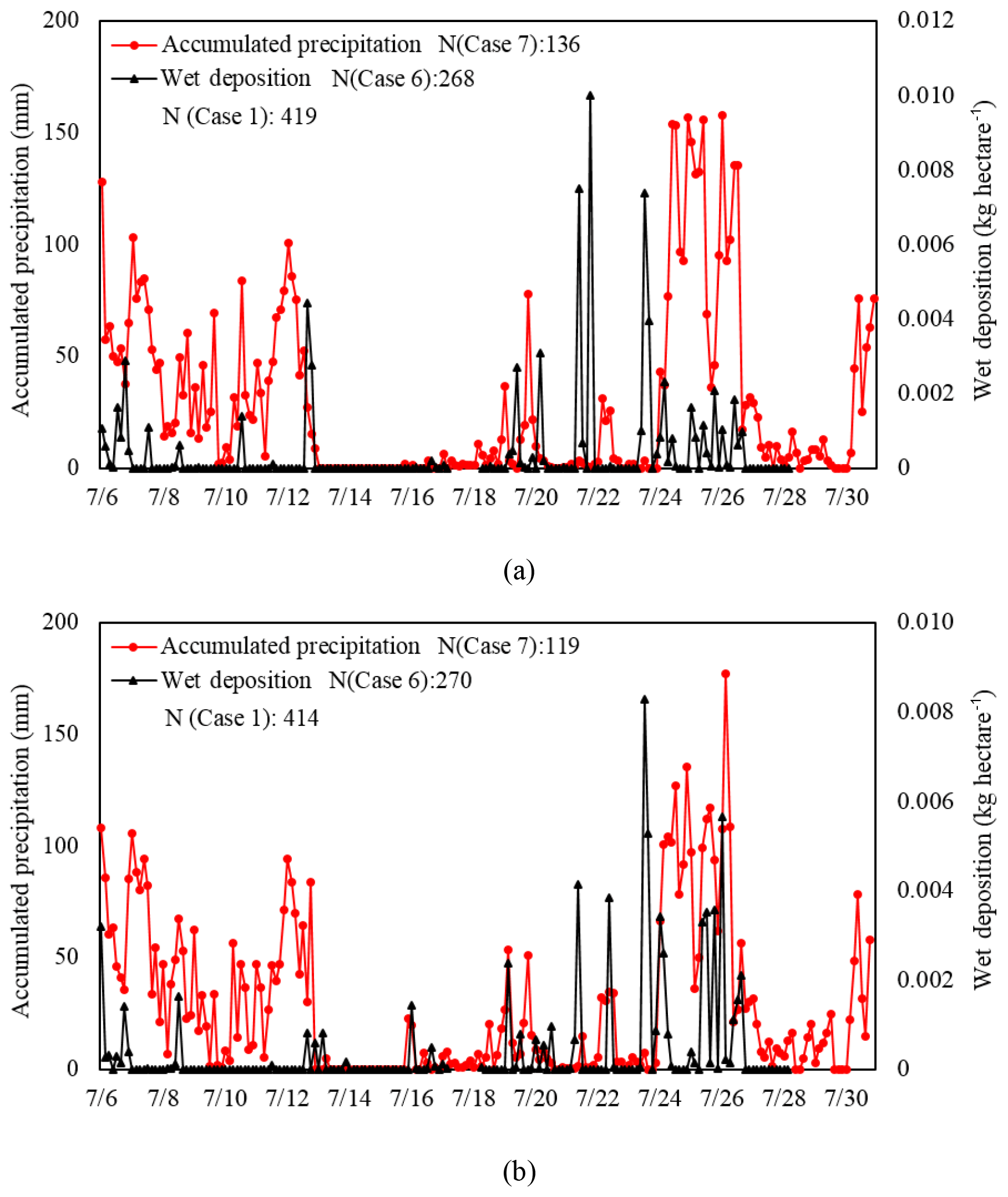
Figure 9The wet deposition in Case 6 (right axis, unit: kg ha−1) and accumulated precipitation in Case 7 (left axis, mm) at NJU (a) and PAES (b). The number of remaining data points is also given.
Table 5 shows the scaling factors estimated from the multiple regression model in Case 7, and no big changes were found compared to the scaling factors for July in Case 6. Consequently, the emissions by sector and total emissions in Case 7 were close to those in Case 6 (Table 6). The relative deviation of total emissions in July between Case 7 and JS-posterior (RD in Table 6) was 13 %, and those for residential and transportation were larger. The influence of precipitation was again indicated modest, as the deviation was much smaller than that between the estimates obtained from the bottom-up and top-down methods. Moreover, the CTM performance based on Case 7, indicated by NMB and NME, was found to be similar to that based on Case 6, implying the small effect of precipitation screening on simulation. Even excluding the influence of precipitation along the back trajectories, the Sig. for residential sources in Case 7 was still much larger than 0.05 (Table 5), suggesting more efforts on quantification of emissions for this highly uncertain source category.
Monthly top-down estimates of BC emissions were derived from a multiple regression model that integrated CTM and hourly BC concentrations from two ground observation sites in the southern Jiangsu city cluster. The annual emissions from the top-down approach (JS-posterior) were estimated at 13.4 Gg for 2015, 50.3 % smaller than those in the bottom-up emission inventory that did not include the improved emission controls in recent years (JS-prior), implying the effectiveness of air pollution prevention measures on emission abatement. Application of JS-posterior in CTM reduced the deviations between simulations and observations at two ground sites effectively, especially at urban site PAES. The increased bias at NJU in certain months reflected the limitation of the top-down estimate. To evaluate the effects of observation data on top-down estimates, two more cases in which observation data of only one site (NJU) and observation data at both sites with their spatial representativeness differentiated were applied to constrain the emissions, respectively. The best CTM performance was found for the third case, indicating that inclusion of more ground measurements with better spatiotemporal coverage in the city cluster would improve the understanding of spatial distributions of BC emissions. In addition, top-down estimates were derived from various bottom-up inventories, and the differences in emission amount, spatial distribution, and CTM performance between the constrained emission estimates were significantly reduced compared to those between the bottom-up inventories. The results implied that changes in the a priori emission input in the regression model and CTM had a limited effect on the top-down estimation. Finally, the assumption of near-linearity between emissions and concentrations was justified, and the influence of wet deposition on the estimated emissions was evaluated to be moderate. This work demonstrated that the top-down approach based on ground observations and CTM could capture the fast changes in BC emissions attributed to tightened pollution control policy at a city cluster scale. To further reduce the uncertainty of the approach and apply the method to other regions, more ground measurements with sufficient temporal resolution would be recommended.
The Multi-resolution Emission Inventory for China used in this study was obtained at http://www.meicmodel.org/ (last access: 12 February 2019, Tsinghua University, 2012). The high-resolution inventory for 2012 in Jiangsu province was obtained in Zhou et al. (2017) and can be accessed at http://www.airqualitynju.com/ (last access: 12 February 2019). The merged high-quality precipitation was obtained by the Tropical Rainfall Measuring Mission satellite instrument at https://trmm.gsfc.nasa.gov/ (last access: 12 February 2019, NASA, 2015).
The supplement related to this article is available online at: https://doi.org/10.5194/acp-19-2095-2019-supplement.
XZ developed the model, wrote the draft, and produced all the figures and tables. YZ provided useful comments and revised the paper. DC, CL, and JZ provided observation data of BC concentrations.
The authors declare that they have no conflict of interest.
This work was sponsored by the Natural Science Foundation of China (91644220
and 41575142) and the National Key Research and Development Program of China
(2017YFC0210106 and 2016YFC0201507). We would like to acknowledge Tong Dan
from Tsinghua University for national emission data (MEIC).
Edited by: Qiang Zhang
Reviewed by: three
anonymous referees
Annor, T., Lamptey, B., Wagner, S., Oguntunde, P., Arnault, J., Heinzeller, D., and Kunstmann, H.: High-resolution long-term WRF climate simulations over Volta Basin. Part 1: validation analysis for temperature and precipitation, Theor. Appl. Climatol., 133, 829–849, https://doi.org/10.1007/s00704-017-2223-5, 2017.
Baker, K., Johnson, M., and King, S.: Meteorological modeling performance summary for application to PM2.5/haze/ozone modeling projects, Lake Michigan Air Directors Consortium, Midwest Regional Planning Organization, Des Plaines, Illinois, USA, 57 pp., 2004.
Bond, T. C., Streets, D. G., Yarber, K. F., Nelson, S. M., Woo, J. H., and Klimont, Z.: A technology-based global inventory of black and organic carbon emissions from combustion, J. Geophys. Res.-Atmos., 109, D14203, https://doi.org/10.1029/2003jd003697, 2004.
Bond, T. C., Doherty, S. J., Fahey, D. W., Forster, P. M., Berntsen, T., DeAngelo, B. J., Flanner, M. G., Ghan, S., Kaercher, B., Koch, D., Kinne, S., Kondo, Y., Quinn, P. K., Sarofim, M. C., Schultz, M. G., Schulz, M., Venkataraman, C., Zhang, H., Zhang, S., Bellouin, N., Guttikunda, S. K., Hopke, P. K., Jacobson, M. Z., Kaiser, J. W., Klimont, Z., Lohmann, U., Schwarz, J. P., Shindell, D., Storelvmo, T., Warren, S. G., and Zender, C. S.: Bounding the role of black carbon in the climate system: A scientific assessment, J. Geophys. Res.-Atmos., 118, 5380–5552, https://doi.org/10.1002/jgrd.50171, 2013.
Cao, G., Zhang, X., and Zheng, F.: Inventory of black carbon and organic carbon emissions from China, Atmos. Environ., 40, 6516–6527, https://doi.org/10.1016/j.atmosenv.2006.05.070, 2006.
Chen, D., Cui, H., Zhao, Y., Yin, L., Lu, Y., and Wang, Q.: A two-year study of carbonaceous aerosols in ambient PM2.5 at a regional background site for western Yangtze River Delta, China, Atmos. Res., 183, 351–361, https://doi.org/10.1016/j.atmosres.2016.09.004, 2017.
Cohen, J. B. and Wang, C.: Estimating global black carbon emissions using a top-down Kalman Filter approach, J. Geophys. Res.-Atmos., 119, 307–323, https://doi.org/10.1002/2013jd019912, 2014.
Dachs, J. and Eisenreich, S. J.: Adsorption onto aerosol soot carbon dominates gas-particle partitioning of polycyclic aromatic hydrocarbons, Eniron. Sci. Technol., 34, 3690–3697, https://doi.org/10.1021/es991201+, 2000.
EEA (European Environment Agency): COPERT 4-Computer Programme to Calculate Emissions from Road Transport, User Manual (Version 9.0), Copenhagen, Denmark, 2012.
Emery, C., Tai, E., and Yarwood, G.: Enhanced meteorological modeling and performance evaluation for two Texas ozone episodes, Final Report, ENVIRON, Texas Natural Resource Conservation Commission, 2001.
Fu, T.-M., Cao, J. J., Zhang, X. Y., Lee, S. C., Zhang, Q., Han, Y. M., Qu, W. J., Han, Z., Zhang, R., Wang, Y. X., Chen, D., and Henze, D. K.: Carbonaceous aerosols in China: top-down constraints on primary sources and estimation of secondary contribution, Atmos. Chem. Phys., 12, 2725–2746, https://doi.org/10.5194/acp-12-2725-2012, 2012.
García-Díez, M., Fernández, J., and Vautard, R.: An RCM multi-physics ensemble over Europe: multi-variable evaluation to avoid error compensation, Clim. Dynam., 45, 3141–3156, https://doi.org/10.1007/s00382-015-2529-x, 2015.
Gilardoni, S., Vignati, E., and Wilson, J.: Using measurements for evaluation of black carbon modeling, Atmos. Chem. Phys., 11, 439–455, https://doi.org/10.5194/acp-11-439-2011, 2011.
Guerrette, J. J. and Henze, D. K.: Four-dimensional variational inversion of black carbon emissions during ARCTAS-CARB with WRFDA-Chem, Atmos. Chem. Phys., 17, 7605–7633, https://doi.org/10.5194/acp-17-7605-2017, 2017.
Hong, C., Zhang, Q., He, K., Guan, D., Li, M., Liu, F., and Zheng, B.: Variations of China's emission estimates: response to uncertainties in energy statistics, Atmos. Chem. Phys., 17, 1227–1239, https://doi.org/10.5194/acp-17-1227-2017, 2017.
Hu, Z., Zhao, C., Huang, J., Leung, L. R., Qian, Y., Yu, H., Huang, L., and Kalashnikova, O. V.: Trans-Pacific transport and evolution of aerosols: evaluation of quasi-global WRF-Chem simulation with multiple observations, Geosci. Model Dev., 9, 1725–1746, https://doi.org/10.5194/gmd-9-1725-2016, 2016.
Huang, Y., Zhao, Y., Qiu, L., Xie, F., Zhang, J., and Huang, X.: The impacts of emission control and meteorology variation on reduced ambient PM2.5 concentrations for a typical industrial city in Yangtze River Delta, China, in preparation, 2019.
Jacobson, M. Z.: Strong radiative heating due to the mixing state of black carbon in atmospheric aerosols, Nature, 409, 695–697, https://doi.org/10.1038/35055518, 2001.
Kaewmesri, P.: The Performance of Microphysics Scheme in Wrf Model for Simulating Extreme Rainfall Events, Int. J. GEOMATE, 15, 121–131, https://doi.org/10.21660/2018.51.59256, 2018.
Koch, D., Schulz, M., Kinne, S., McNaughton, C., Spackman, J. R., Balkanski, Y., Bauer, S., Berntsen, T., Bond, T. C., Boucher, O., Chin, M., Clarke, A., De Luca, N., Dentener, F., Diehl, T., Dubovik, O., Easter, R., Fahey, D. W., Feichter, J., Fillmore, D., Freitag, S., Ghan, S., Ginoux, P., Gong, S., Horowitz, L., Iversen, T., Kirkevåg, A., Klimont, Z., Kondo, Y., Krol, M., Liu, X., Miller, R., Montanaro, V., Moteki, N., Myhre, G., Penner, J. E., Perlwitz, J., Pitari, G., Reddy, S., Sahu, L., Sakamoto, H., Schuster, G., Schwarz, J. P., Seland, Ø., Stier, P., Takegawa, N., Takemura, T., Textor, C., van Aardenne, J. A., and Zhao, Y.: Evaluation of black carbon estimations in global aerosol models, Atmos. Chem. Phys., 9, 9001–9026, https://doi.org/10.5194/acp-9-9001-2009, 2009.
Kondo, Y., Oshima, N., Kajino, M., Mikami, R., Moteki, N., Takegawa, N., Verma, R. L., Kajii, Y., Kato, S., and Takami, A.: Emissions of black carbon in East Asia estimated from observations at a remote site in the East China Sea, J. Geophys. Res.-Atmos., 116, D16201, https://doi.org/10.1029/2011jd015637, 2011.
Kotlarski, S., Keuler, K., Christensen, O. B., Colette, A., Déqué, M., Gobiet, A., Goergen, K., Jacob, D., Lüthi, D., van Meijgaard, E., Nikulin, G., Schär, C., Teichmann, C., Vautard, R., Warrach-Sagi, K., and Wulfmeyer, V.: Regional climate modeling on European scales: a joint standard evaluation of the EURO-CORDEX RCM ensemble, Geosci. Model Dev., 7, 1297–1333, https://doi.org/10.5194/gmd-7-1297-2014, 2014.
Kurokawa, J., Ohara, T., Morikawa, T., Hanayama, S., Janssens-Maenhout, G., Fukui, T., Kawashima, K., and Akimoto, H.: Emissions of air pollutants and greenhouse gases over Asian regions during 2000–2008: Regional Emission inventory in ASia (REAS) version 2, Atmos. Chem. Phys., 13, 11019–11058, https://doi.org/10.5194/acp-13-11019-2013, 2013.
Lei, Y., Zhang, Q., He, K. B., and Streets, D. G.: Primary anthropogenic aerosol emission trends for China, 1990–2005, Atmos. Chem. Phys., 11, 931–954, https://doi.org/10.5194/acp-11-931-2011, 2011.
Li, L., Chen, C. H., Fu, J. S., Huang, C., Streets, D. G., Huang, H. Y., Zhang, G. F., Wang, Y. J., Jang, C. J., Wang, H. L., Chen, Y. R., and Fu, J. M.: Air quality and emissions in the Yangtze River Delta, China, Atmos. Chem. Phys., 11, 1621–1639, https://doi.org/10.5194/acp-11-1621-2011, 2011.
Li, N., Fu, T.-M., Cao, J. J., Zheng, J. Y., He, Q. Y., Long, X., Zhao, Z. Z., Cao, N. Y., Fu, J. S., and Lam, Y. F.: Observationally-constrained carbonaceous aerosol source estimates for the Pearl River Delta area of China, Atmos. Chem. Phys. Discuss., 15, 33583–33629, https://doi.org/10.5194/acpd-15-33583-2015, 2015.
Li, N., He, Q., Tie, X., Cao, J., Liu, S., Wang, Q., Li, G., Huang, R., and Zhang, Q.: Quantifying sources of elemental carbon over the Guanzhong Basin of China: A consistent network of measurements and WRF-Chem modeling, Environ. Pollut., 214, 86–93, https://doi.org/10.1016/j.envpol.2016.03.046, 2016.
Liu, D., Yang, B., Zhang, Y., Qian, Y., Huang, A., Zhou, Y., and Zhang, L.: Combined impacts of convection and microphysics parameterizations on the simulations of precipitation and cloud properties over Asia, Atmos. Res., 212, 172–185, https://doi.org/10.1016/j.atmosres.2018.05.017, 2018.
Liu, M., Lin, J., Wang, Y., Sun, Y., Zheng, B., Shao, J., Chen, L., Zheng, Y., Chen, J., Fu, T.-M., Yan, Y., Zhang, Q., and Wu, Z.: Spatiotemporal variability of NO2 and PM2.5 over Eastern China: observational and model analyses with a novel statistical method, Atmos. Chem. Phys., 18, 12933–12952, https://doi.org/10.5194/acp-18-12933-2018, 2018.
Lu, Z., Zhang, Q., and Streets, D. G.: Sulfur dioxide and primary carbonaceous aerosol emissions in China and India, 1996–2010, Atmos. Chem. Phys., 11, 9839–9864, https://doi.org/10.5194/acp-11-9839-2011, 2011.
Malm, W. C., Sisler, J. F., Huffman, D., Eldred, R. A., and Cahill, T. A.: Spatial and seasonal trends in particle concentration and optical extinction in the United States, J. Geophys. Res.-Atmos., 99, 1347–1370, https://doi.org/10.1029/93jd02916, 1994.
Matsui, H., Koike, M., Kondo, Y., Oshima, N., Moteki, N., Kanaya, Y., Takami, A., and Irwin, M.: Seasonal variations of Asian black carbon outflow to the Pacific: Contribution from anthropogenic sources in China and biomass burning sources in Siberia and Southeast Asia, J. Geophys. Res.-Atmos., 118, 9948–9967, https://doi.org/10.1002/jgrd.50702, 2013.
National Aeronautics and Space Administration (NASA): the merged high-quality precipitation obtained by the Tropical Rainfall Measuring Mission satellite instrument (TRMM), available at: https://trmm.gsfc.nasa.gov/ (last access: 12 February 2019), 2015.
Ohara, T., Akimoto, H., Kurokawa, J., Horii, N., Yamaji, K., Yan, X., and Hayasaka, T.: An Asian emission inventory of anthropogenic emission sources for the period 1980–2020, Atmos. Chem. Phys., 7, 4419–4444, https://doi.org/10.5194/acp-7-4419-2007, 2007.
Park, R. J.: Sources of carbonaceous aerosols over the United States and implications for natural visibility, J. Geophys. Res., 108, 4355, https://doi.org/10.1029/2002jd003190, 2003.
Politi, N., Nastos, P. T., Sfetsos, A., Vlachogiannis, D., and Dalezios, N. R.: Evaluation of the AWR-WRF model configuration at high resolution over the domain of Greece, Atmos. Res., 208, 229–245, https://doi.org/10.1016/j.atmosres.2017.10.019, 2018.
Qian, W.: Air Pollution Control Planning for the Key Regions during the 12th Five-Year Plan period (2010–2015), China Environmental Protection Industry, 4–18, 2013.
Qin, Y. and Xie, S. D.: Spatial and temporal variation of anthropogenic black carbon emissions in China for the period 1980–2009, Atmos. Chem. Phys., 12, 4825–4841, https://doi.org/10.5194/acp-12-4825-2012, 2012.
Ramanathan, V. and Carmichael, G.: Global and regional climate changes due to black carbon, Nat. Geosci., 1, 221–227, https://doi.org/10.1038/ngeo156, 2008.
Streets, D. G., Gupta, S., Waldhoff, S. T., Wang, M. Q., Bond, T. C., and Bo, Y. Y.: Black carbon emissions in China, Atmos. Environ., 35, 4281–4296, https://doi.org/10.1016/s1352-2310(01)00179-0, 2001.
Streets, D. G., Bond, T. C., Carmichael, G. R., Fernandes, S. D., Fu, Q., He, D., Klimont, Z., Nelson, S. M., Tsai, N. Y., Wang, M. Q., Woo, J. H., and Yarber, K. F.: An inventory of gaseous and primary aerosol emissions in Asia in the year 2000, J. Geophys. Res.-Atmos., 108, 8809, https://doi.org/10.1029/2002jd003093, 2003.
Tsinghua University: Multi-resolution Emission Inventory for China (MEIC), available at: http://www.meicmodel.org/ (last access: 12 February 2019), 2012.
Verma, S., Reddy, D. M., Ghosh, S., Kumar, D. B., and Chowdhury, A. K.: Estimates of spatially and temporally resolved constrained black carbon emission over the Indian region using a strategic integrated modelling approach, Atmos. Res., 195, 9–19, https://doi.org/10.1016/j.atmosres.2017.05.007, 2017.
Wang, Y., Wang, X., Kondo, Y., Kajino, M., Munger, J. W., and Hao, J.: Black carbon and its correlation with trace gases at a rural site in Beijing: Top-down constraints from ambient measurements on bottom-up emissions, J. Geophys. Res.-Atmos., 116, D24304, https://doi.org/10.1029/2011jd016575, 2011.
Wang, X., Wang, Y., Hao, J., Kondo, Y., Irwin, M., Munger, J. W., and Zhao, Y.: Top-down estimate of China's black carbon emissions using surface observations: Sensitivity to observation representativeness and transport model error, J. Geophys. Res.-Atmos., 118, 5781–5795, https://doi.org/10.1002/jgrd.50397, 2013.
Xia, Y., Zhao, Y., and Nielsen, C. P.: Benefits of of China's efforts in gaseous pollutant control indicated by the bottom-up emissions and satellite observations 2000-2014, Atmos. Environ., 136, 43–53, https://doi.org/10.1016/j.atmosenv.2016.04.013, 2016.
Xu, X., Wang, J., Henze, D. K., Qu, W., and Kopacz, M.: Constraints on aerosol sources using GEOS-Chem adjoint and MODIS radiances, and evaluation with multisensor (OMI, MISR) data, J. Geophys. Res.-Atmos., 118, 10139–10139, https://doi.org/10.1002/jgrd.50784, 2013.
Yang, B., Zhang, Y., Qian, Y., Huang, A., and Yan, H.: Calibration of a convective parameterization scheme in the WRF model and its impact on the simulation of East Asian summer monsoon precipitation, Clim. Dynam., 44, 1661–1684, https://doi.org/10.1007/s00382-014-2118-4, 2014.
Yu, E., Wang, H., Gao, Y., and Sun, J.: Impacts of cumulus convective parameterization schemes on summer monsoon precipitation simulation over China, Acta Meteorol. Sin., 25, 581–592, https://doi.org/10.1007/s13351-011-0504-y, 2011.
Zhang, L., Henze, D. K., Grell, G. A., Carmichael, G. R., Bousserez, N., Zhang, Q., Torres, O., Ahn, C., Lu, Z., Cao, J., and Mao, Y.: Constraining black carbon aerosol over Asia using OMI aerosol absorption optical depth and the adjoint of GEOS-Chem, Atmos. Chem. Phys., 15, 10281–10308, https://doi.org/10.5194/acp-15-10281-2015, 2015.
Zhang, Q., Streets, D. G., Carmichael, G. R., He, K. B., Huo, H., Kannari, A., Klimont, Z., Park, I. S., Reddy, S., Fu, J. S., Chen, D., Duan, L., Lei, Y., Wang, L. T., and Yao, Z. L.: Asian emissions in 2006 for the NASA INTEX-B mission, Atmos. Chem. Phys., 9, 5131–5153, https://doi.org/10.5194/acp-9-5131-2009, 2009.
Zhang, Y., Liu, P., Pun, B., and Seigneur, C.: A comprehensive performance evaluation of MM5-CMAQ for the Summer 1999 Southern Oxidants Study episode – Part I: Evaluation protocols, databases, and meteorological predictions, Atmos. Environ., 40, 4825–4838, https://doi.org/10.1016/j.atmosenv.2005.12.043, 2006.
Zhao, Y., Zhang, J., and Nielsen, C. P.: The effects of recent control policies on trends in emissions of anthropogenic atmospheric pollutants and CO2 in China, Atmos. Chem. Phys., 13, 487–508, https://doi.org/10.5194/acp-13-487-2013, 2013.
Zhao, Y., Zhang, J., and Nielsen, C. P.: The effects of energy paths and emission controls and standards on future trends in China's emissions of primary air pollutants, Atmos. Chem. Phys., 14, 8849–8868, https://doi.org/10.5194/acp-14-8849-2014, 2014.
Zhao, Y., Zhou, Y., Qiu, L., and Zhang, J.: Quantifying the uncertainties of China's emission inventory for industrial sources: From national to provincial and city scales, Atmos. Environ., 165, 207–221, https://doi.org/10.1016/j.atmosenv.2017.06.045, 2017.
Zheng, J., He, M., Shen, X., Yin, S., and Yuan, Z.: High resolution of black carbon and organic carbon emissions in the Pearl River Delta region, China, Sci. Total Environ., 438, 189–200, https://doi.org/10.1016/j.scitotenv.2012.08.068, 2012.
Zhou, Y., Zhao, Y., Mao, P., Zhang, Q., Zhang, J., Qiu, L., and Yang, Y.: Development of a high-resolution emission inventory and its evaluation and application through air quality modeling for Jiangsu Province, China, Atmos. Chem. Phys., 17, 211–233, https://doi.org/10.5194/acp-17-211-2017, 2017.