the Creative Commons Attribution 4.0 License.
the Creative Commons Attribution 4.0 License.
 | 08 Feb 2019
Turbulent enhancement of radar reflectivity factor for polydisperse cloud droplets
Ryo Onishi
The radar reflectivity factor is important for estimating cloud microphysical properties; thus, in this study, we determine the quantitative influence of microscale turbulent clustering of polydisperse droplets on the radar reflectivity factor. The theoretical solution for particulate Bragg scattering is obtained without assuming monodisperse droplet sizes. The scattering intensity is given by an integral function including the cross spectrum of number density fluctuations for two different droplet sizes. We calculate the cross spectrum based on turbulent clustering data, which are obtained by the direct numerical simulation (DNS) of particle-laden homogeneous isotropic turbulence. The results show that the coherence of the cross spectrum is close to unity for small wave numbers and decreases almost exponentially with increasing wave number. This decreasing trend is dependent on the combination of Stokes numbers. A critical wave number is introduced to characterize the exponential decrease of the coherence and parameterized using the Stokes number difference. Comparison with DNS results confirms that the proposed model can reproduce the -weighted power spectrum, which is proportional to the clustering influence on the radar reflectivity factor to a sufficiently high accuracy. Furthermore, the proposed model is extended to incorporate the gravitational settling influence by modifying the critical wave number based on the analytical equation derived for the bidisperse radial distribution function. The estimate of the modified model also shows good agreement with the DNS results for the case with gravitational droplet settling. The model is then applied to high-resolution cloud-simulation data obtained from a spectral-bin cloud simulation. The result shows that the influence of turbulent clustering can be significant inside turbulent clouds. The large influence is observed at the near-top of the clouds, where the liquid water content and the energy dissipation rate are sufficiently large.
- Article
(3712 KB) - Full-text XML
- BibTeX
- EndNote


Radar remote sensing is widely used for observing a spatial distribution of cloud and precipitation particles because it can also provide estimates of cloud microphysical properties. The remote-sensing data are analyzed and displayed using the radar reflectivity factor (mm6 m−3), Z, which is obtained with the following radar equation:
where Pr and Pt are the received and transmitted microwave powers, G is the antenna gain, Ae is the effective aperture of the antenna, km is the microwave wave number, K is the dielectric coefficient of a water droplet, V is the measurement volume, and R is the distance between the antenna and the cloud. The relationship between the radar reflectivity factor and cloud microphysical properties is usually expressed based on the assumption of incoherent scattering (Gossard and Strauch, 1983). Incoherent scattering implies random and uniform dispersion of cloud droplets (Bohren and Huffman, 1983). For this case, the factor is proportional to the sum of the scattering intensities of the individual droplets in the measurement volume. In contrast, droplets form a nonuniform spatial distribution in turbulence; i.e., inertial particles concentrate in small-enstrophy regions during turbulence due to the centrifugal motion (Maxey, 1987; Squires and Eaton, 1991; Wang and Maxey, 1993; Chen et al., 2006). This preferential concentration is often referred to as turbulent clustering. Nonuniform distribution of cloud droplets results in coherent scattering, which is also referred to as particulate Bragg scattering (Kostinski and Jameson, 2000). For this case, the interference of microwaves scattered by nonuniformly distributed droplets increases the scattered microwave intensity; i.e., the radar reflectivity factor increases due to particulate Bragg scattering. It should be noted that Bragg scattering often indicates coherent scattering due to a nonuniform distribution of the refractive index of clear air. In the troposphere, turbulent mixing of temperature and water vapor causes spatial variation of the refractive index. To distinguish this effect from the particulate Bragg scattering, it is specifically referred to as clear-air Bragg scattering. The radar reflectivity factor for both types of Bragg scattering is dependent on the microwave frequency fm (, where c is the speed of light), while the factor for incoherent scattering is independent of fm. Knight and Miller (1998) reported radar frequency dependence of their observation results for small warm cumulus clouds using S- and X-band microwaves, which have wavelengths of 10 and 3 cm, respectively. Their observation data of S-band radar show a characteristic echo pattern of the mantle echo, in which a strong radar echo was observed in cloud edges, while it is relatively weak in cloud core regions. The mantle echo can be explained by clear-air Bragg scattering, since the radar reflectivity factor difference is about 19 dB as expected for ideal Bragg scattering. They also reported that there are many cases in which frequency dependence is not explained by clear-air Bragg scattering. In such cases, the S-band radar echo is about 10 dB stronger than the X-band radar echo, and the difference is also observed in the cloud core regions. Rogers and Brown (1997) also reported a similar frequency dependence of radar returns during their observation of a smoke plume from intense fire, using a UHF wind profiler and an X-band radar. Erkelens et al. (2001) analyzed the observation data and estimated the influence of coherent scattering by cloud droplets using the power law of turbulent spectrum, which represents turbulent mixing of cloud water with environmental clear air, i.e., turbulent entrainment. They concluded that coherent scattering by cloud droplets can be more significant than clear-air Bragg scattering, whereas turbulent entrainment is not the only factor relevant to the frequency dependence in the observation data. Kostinski and Jameson (2000) first pointed out the possibility that particulate Bragg scattering due to turbulent clustering leads to the frequency dependence reported by Knight and Miller (1998). To evaluate the quantitative influence of turbulent clustering on the radar reflectivity factor, it is crucial to understand the spatial structure of turbulent clustering. Turbulent clustering has been discussed in much of the literature because it can enhance the collision growth of cloud droplets (e.g., Sundaram and Collins, 1997; Reade and Collins, 2000; Ayala et al., 2008a, b; Onishi et al., 2009; Wang et al., 2009; Onishi and Vassilicos, 2014), and statistical data on turbulent clustering have been obtained for scales relevant to droplet collisions. However, these data cannot be adopted for particulate Bragg scattering because the clustering scales relevant to particulate Bragg scattering are on the microwave wavelength, which is larger than droplet collision scales. A quantitative estimate of particulate Bragg scattering due to turbulent clustering is first provided by Dombrovsky and Zaichik (2010). Their analytical estimate was based on a clustering model for droplet collision scales but indicated that turbulent clustering can lead to a considerable increase in the radar reflectivity factor. Matsuda et al. (2014) clarified the quantitative influence based on turbulent clustering data obtained by a three-dimensional direct numerical simulation (DNS), which covered the clustering scales on the microwave wavelength. They estimated the increase in the radar reflectivity factor due to turbulent clustering by calculating the power spectrum of number density fluctuations, Enp(k|rp), where k is the wave number and rp is the droplet radius. The power spectrum Enp(k|rp) is strongly dependent on the droplet size: more specifically, Enp(k|rp) is dependent on the Stokes number, St, which is defined as (τp is the relaxation time of droplet motion and τη is the Kolmogorov time). However, the discussion of radar reflectivity factor increases is limited to cases of monodisperse particles. Thus, the results are not directly applicable to particulate Bragg scattering for real cloud systems, in which cloud droplets have broad droplet size distributions.
Therefore, this study aims to investigate the influence of turbulent clustering of polydisperse droplets on particulate Bragg scattering. Firstly, the theoretical formulation of particulate Bragg scattering is extended for polydisperse particles and expressed using the cross spectrum of number density fluctuations for two different droplet sizes. Secondly, the three-dimensional DNS of particle-laden homogeneous isotropic turbulence is performed to obtain turbulent droplet clustering data, which are used to calculate the power spectrum and the cross spectrum of number density fluctuations. A parameterization for the cross spectrum is then proposed considering the dependence of the Stokes number combination, and the influence of gravitational settling is discussed and incorporated. Finally, in order to investigate the impact of turbulent clustering on radar observations of realistic clouds, the proposed model is applied to high-resolution cloud-simulation data obtained by a spectral-bin cloud microphysics simulation.
Here, we aim to formulate the radar reflectivity factor Z for a nonuniform distribution of polydisperse cloud droplets based on the discussion of Gossard and Strauch (1983), but without assuming monodisperse droplet sizes. Because the radii of cloud droplets are much smaller than the microwave wavelength, the electric field vector of the microwaves scattered by a single droplet, Esca(t, x,rp), is given by the Rayleigh-scattering approximation:
where Einc is the electric field amplitude vector of the incident microwave; rp is the droplet radius; x, xt, and xr are the position vectors of the droplet, microwave transmitter, and microwave receiver; kinc and ksca are the wave number vectors of the incident and scattered microwaves which satisfy , and χ is the angle between Einc and ksca. Considering the droplet-size dependence of Esca(t, x, rp), the electric power of the microwave scattered by a group of droplets, Ps, is given by
where n(x, rp)drpdx is the number of droplets with radii from rp to in an infinitesimal volume dx at position x, and ζ is the intrinsic impedance. The overbar denotes the temporal average. The relationship between the radar reflectivity factor Z and the scattering properties of target clouds is given by
where λ is the microwave wavelength and σ is the radar cross section (Gossard and Strauch, 1983), which is defined as
where Po is the electric power of the incident microwave, which is given by . Substitution of Eqs. (2), (3), and (5) into Eq. (4) yields
where the wave number vector κ is defined as . Note that radar remote sensing typically uses backward scattering; i.e., . Thus, κ=2kinc.
Similarly to Gossard and Strauch (1983), we assume n(x, rp) to be composed of the temporal-average and fluctuation parts; i.e., n(x, . The temporal-average part, , contributes to the separated reflection; therefore, the contribution of this part is negligibly small when has no fluctuation on a spatial scale of half the wavelength (Erkelens et al., 2001). Thus, we neglect the contribution of . Then, we obtain
where the angular brackets represent a temporal and spatial average in the measurement volume.
In order to decompose the spatial correlation function , we introduce the probability density function (PDF) of droplet radius rp to the measurement volume, qr(rp), and the number density distribution function for monodisperse droplets with a radius of rp, np(x|rp). The PDF is defined as , where Np is the total number of droplets in the measurement volume; i.e., . The PDF satisfies . The number density distribution function for monodisperse droplets is then defined as so that n(x,rp) is given by . The number density distribution function np(x|rp) satisfies for arbitrary rp. Note that the spatial correlation function for is discontinuous at r=0 because the droplet distribution is composed of spatially discrete points. The singularity is given by , where δ(r) and are the Dirac delta functions. Thus, the spatial correlation function is given by
where 〈np〉 is the average number density () and is defined as the continuous part of . Substitution of Eq. (8) into Eq. (7) and adoption of the isotropic clustering assumption Gossard and Strauch (1983) yield
where κ is , is given by , and Er3np(k) is the -weighted power spectrum, defined as
where is the cross spectrum of number density fluctuations for np(x|rp) and : the cross spectrum is defined as ; i.e., the integration of over the spherical shell, σk, at , in which is the cross spectral density function, defined as
The first and second terms on the right-hand side of Eq. (9) are the incoherent and coherent scattering parts; particulate Bragg scattering is caused by the second term. Equations (9) and (10) imply that the particulate Bragg-scattering part of Z for an arbitrary droplet size distribution can be calculated using the cross spectrum for bidisperse droplet size conditions. When droplets are distributed randomly and uniformly, the second term equals zero. Thus, the radar reflectivity factor when assuming a random and uniform droplet distribution is given by the first term; i.e., .
It should be noted that Eq. (9) satisfies the theoretical solution for particulate Bragg scattering of monodisperse droplets: for the case of monodisperse droplets with radii of rp1, the PDF of droplet radius is given by . Then, the radar reflectivity factor Z is given by
where Enp(k|rp) is the power spectrum of number density fluctuations, which satisfies . Note that Enp(k|rp) is defined as , where is the power spectral density function of np(x|rp), defined as
3.1 Direct numerical simulation
In order to obtain turbulent clustering data for calculating the cross spectrum, we have performed a three-dimensional DNS for particle-laden homogeneous isotropic turbulence. Three-dimensional incompressible turbulent airflows were calculated by solving the continuity and Navier–Stokes equations:
where ui is the flow velocity in the ith direction, p is the pressure, ρa is the air density, ν is the kinematic viscosity, and Fi is the external forcing term. The nonlinear term was discretized by the fourth-order central difference scheme (Morinishi et al., 1998). The time integration was calculated by the second-order Runge–Kutta scheme. The HSMAC method (Hirt and Cook, 1972) was used for velocity-pressure coupling. The external forcing was applied to maintain the intensity of large-scale eddies for wave numbers k in the range (Onishi et al., 2011), where L0 is the representative length scale.
Droplet motions were simulated by Lagrangian point-particle tracking. Here, we assumed that the droplet density ρp is much larger than ρa and the drag term is given based on the Stokes law. The droplet motions were tracked by
where vi and gi are the particle velocity and gravitational acceleration in the ith direction. τp is the droplet relaxation time, which is given by
The effects of turbulent modulation and droplet collision were neglected for simplicity because these effects were typically small in the timescale of τη in clouds.
The computational domain was set as a cube with edge lengths of 2πL0. Periodic boundary conditions were applied in all three directions. A uniform staggered grid was used for discretization. The number of grid points was set to 5123. A Taylor microscale-based turbulent Reynolds number of the obtained flow was Reλ=204, where Reλ is defined as , where lλ is the Taylor microscale and u′ is the rms value of the velocity fluctuation. Note that this value of Reλ is sufficiently large to obtain turbulent clustering data for high Reynolds number turbulence in the wave number range relevant to radar observations (Matsuda et al., 2014) (see Sect. 3.2). The kinematic viscosity, ν, was set to m2 s−1, and the ratio of the droplet density to the air density, ρp∕ρa, was set to 840, assuming 1 atm and 298 K. The total number of droplets, Np, was set to 1.5×10⁷.
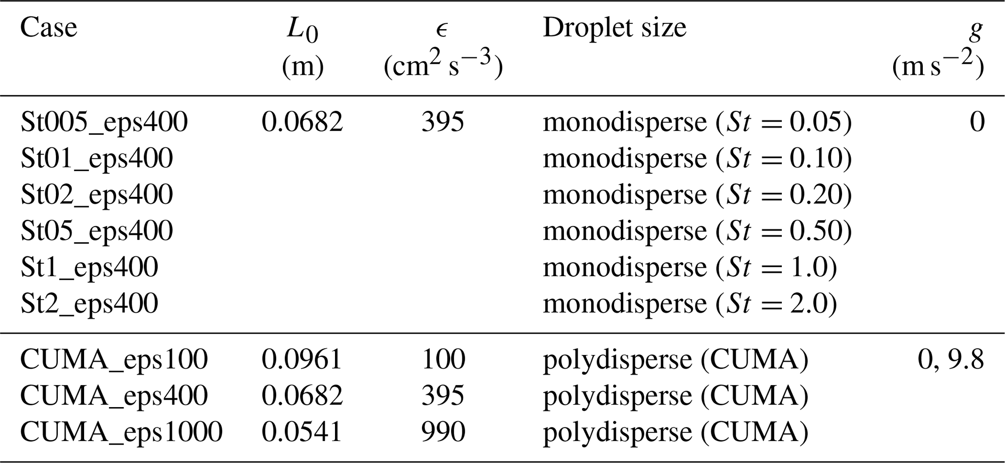
For this study, we performed the DNS for monodisperse and polydisperse droplets. Table 1 shows the computational settings for turbulence, droplet size, and gravitational acceleration. For monodisperse droplets, the droplet motions in an identical turbulent flow field were calculated for six values of Stokes number, St. The clustering data for the monodisperse cases were used for calculating the cross spectrum of number density fluctuations for any combinations of these St values. For polydisperse droplets, a typical droplet size distribution for maritime cumulus clouds (the size distribution data named “CUMA” in Hess et al., 1998) was applied, and the droplets were tracked in turbulent flows using three different energy dissipation rates ϵ. ϵ values of the obtained turbulent flows were approximately 100, 400, and 1000 cm2 s−3, which can be observed in cumulus and cumulonimbus clouds (Pinsky et al., 2008). The data for the polydisperse droplet cases were used to discuss the reliability of the proposed cross spectrum model. It should be noted that the droplet size distribution for the polydisperse cases were identical but the Stokes number histograms were different; the Stokes numbers corresponding to the modal radius (10.4 μm) for ϵ=100, 400, and 1000 cm2 s−3 were 0.035, 0.069, and 0.10, respectively. The gravitational acceleration was set to zero for the monodisperse cases. The DNS for polydisperse droplets were performed under the conditions with and without gravitational settling. The Froude numbers, Fr (, in which is the Kolmogorov acceleration), for the cases with gravitational settling were 0.0520, 0.145, and 0.289 for ϵ=100, 400, and 1000 cm2 s−3, respectively. The influence of gravitational settling on turbulent particle clustering is often discussed using the settling parameter, Sv, which is defined as (e.g., Wang and Maxey, 1993; Grabowski and Vaillancourt, 1999; Bec et al., 2014; Ireland et al., 2016), where vT=τpg is the terminal settling velocity and is the Kolmogorov velocity. Note that Sv satisfies . The settling parameters corresponding to the modal radius for ϵ=100, 400, and 1000 cm2 s−3 were 0.67, 0.48, and 0.38, respectively.
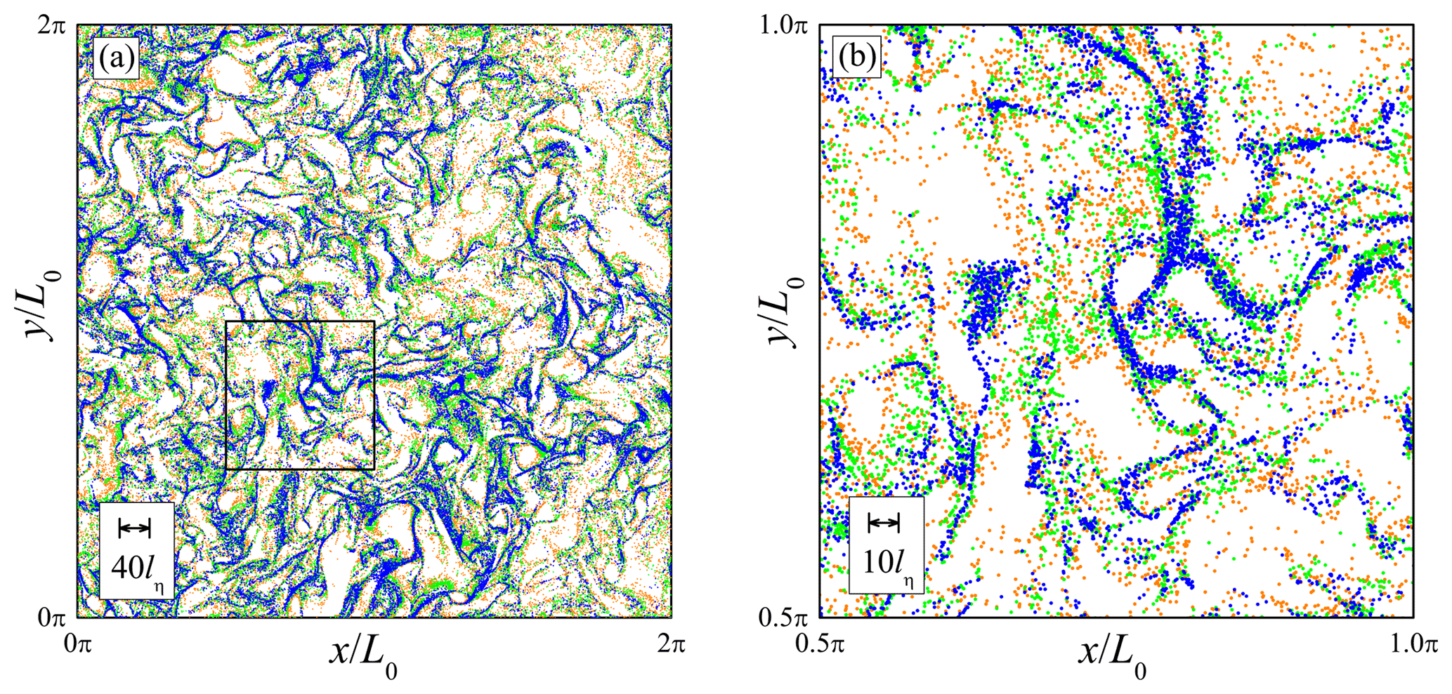
Figure 1Spatial distribution of droplets for (orange) St=0.2, (green) 0.5, and (blue) 1.0 in the regions of (a) 2πL0×2πL0 and (b) 0.5πL0×0.5πL0. Droplets located in the range of are shown. The square frame in (a) corresponds to the region of (b).
3.2 Computation of power spectrum and cross spectrum
The power spectral density function and the cross spectral density function are calculated from the Lagrangian droplet distribution data as follows:
where is the Fourier component of the droplet number density distribution, np(x|rp), and the angle brackets denote an ensemble average. The number density distribution for Lagrangian discrete droplets is given by
where xp,j is the position vector of the jth droplet with radius rp, and Np is the total number of droplets with radius rp. The Fourier components of Eq. (20) are then given by
Substitution of Eq. (21) into Eq. (18) yields
Similarly, substitution of Eq. (21) into Eq. (19) yields
where 〈np1〉 and 〈np2〉 are the average number density of droplets with radii of rp1 and rp2 (i.e., and ), respectively, Np1 and Np2 are the numbers of droplets with radii of rp1 and rp2, respectively, xp1,j is the position of the jth droplet with a radius of rp1, and is the position of the j′th droplet with a radius of rp2. It should be noted that the imaginary part of is omitted in Eq. (25) because, statistically, it should be zero. We confirmed that the imaginary part of calculated from the DNS data is O(10−4), which is caused by the statistical and truncation errors.
The spectral density functions, and , were calculated for discrete wave numbers , where h1, h2, and h3 are arbitrary integers that satisfy , where Δk was set to 1∕L0. Enp(k|rp) and were then obtained by the following equations:
The spectra, Enp(k|rp) and , were calculated for 19 representative wave numbers in the same way as Matsuda et al. (2014). The ensemble average in Eq. (23) was obtained by averaging 10 temporal slices of the droplet distributions, which were sampled for intervals of . The ensemble average in Eq. (25) was also obtained for 10 pairs of temporal slices. Each pair was composed of temporal slices at the same time step for different St cases.

Figure 2Normalized cross spectra , St2) of droplet number density fluctuations compared to normalized power spectra .
Matsuda et al. (2014) normalized the power spectrum Enp(k|rp) by using 〈np〉 and the Kolmogorov scale, lη, defined as , and confirmed that, for Reλ≥204, the Reλ dependence of the normalized power spectrum is negligible at the wave number range relevant to radar observations (). Thus, this study used the same normalization for Enp(k|rp) and as follows:
where ξ is the normalized wave number defined as ξ≡klη and St, St1, and St2 are the Stokes numbers of water droplets with radii of rp, rp1, and rp2.
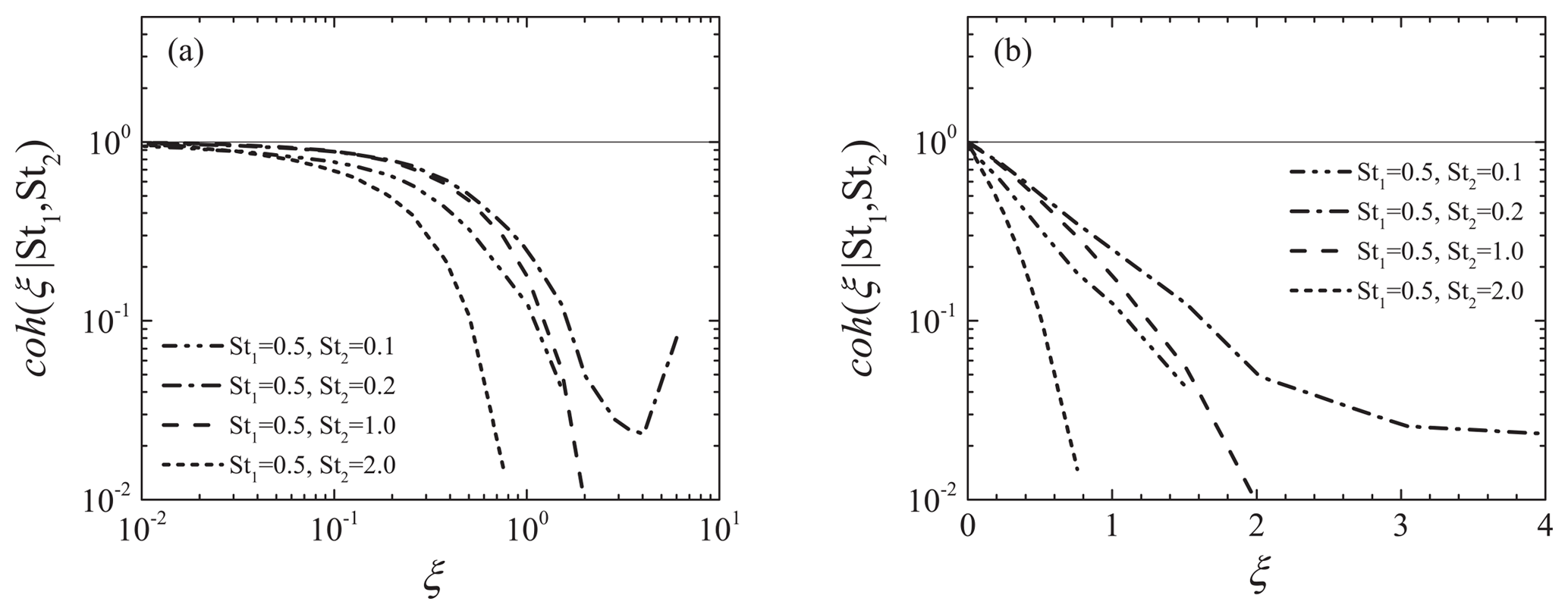
Figure 3Coherence of cross spectra for combinations of St1=0.5 and other Stokes numbers. The same coherence is plotted in (a) a double logarithmic chart and (b) a vertically logarithmic chart.
4.1 Spatial droplet distribution and cross spectrum
Figure 1 shows the spatial distribution of droplets for St=0.2, 0.5, and 1.0. Droplets located in the range of are indicated. The droplet position data were sampled at the same time step; i.e., the background turbulent flow field is identical. Figure 1a is the overall view of the region with a size of 2πL0×2πL0, while Fig. 1b is the magnified view for the region with a size of 0.5πL0×0.5πL0. The clusters and void areas are clearly observed for all St cases. Their location for St=0.5 is almost the same as that for the other St. This is because the locations of clusters and void areas for small St are strongly dependent on the instantaneous turbulent flow field. However, the small-scale structure of clusters is not exactly the same; i.e., the droplets become more concentrated in clusters as St increases. Figure 2 shows the power spectra and the cross spectra obtained from the DNS data. Note that the high wave number portion is omitted when the value of the cross spectrum is smaller than the computational error level (10−4). The power spectra show power-law-type slopes at wave numbers smaller and larger than the peak location. The peak height and slope of the spectra are strongly dependent on the Stokes number; this Stokes number dependence was discussed by Matsuda et al. (2014). In the small wave number region, the cross spectra also show power-law-type slopes. In this region, the curve of for St1=0.5 and St2=0.2 is located between the power spectra for St=0.5 and St=0.2. Similarly, the curve of for St1=0.5 and St2=1.0 is located between the power spectra for St=0.5 and St=1.0. On the other hand, in the large wave number region, both cross spectra become smaller than the power spectra without showing power-law-type slopes. These trends imply that the cross spectrum is influenced by not only the Stokes number dependence of the clustering intensity, but also the spatial correlation of clusters between different values of St. In order to focus on the influence of the spatial correlation of clusters, we have evaluated the coherence , which is defined as
Figure 3 shows the coherence between St1=0.5 and other Stokes numbers. The coherence is close to unity in the small wave number region and decreases to zero as the wave number increases. These trends correspond to the spatial correlation between cluster locations for different St cases in Fig. 1. Figure 3b shows that the coherence decreases with an almost constant slope in the vertically logarithmic and horizontally linear chart. The slope of the coherence is dependent on the combination of St1 and St2; the slope becomes steeper as the difference in St increases. These results indicate that the decreasing trend of coherence can be approximated by an exponential function; i.e.,
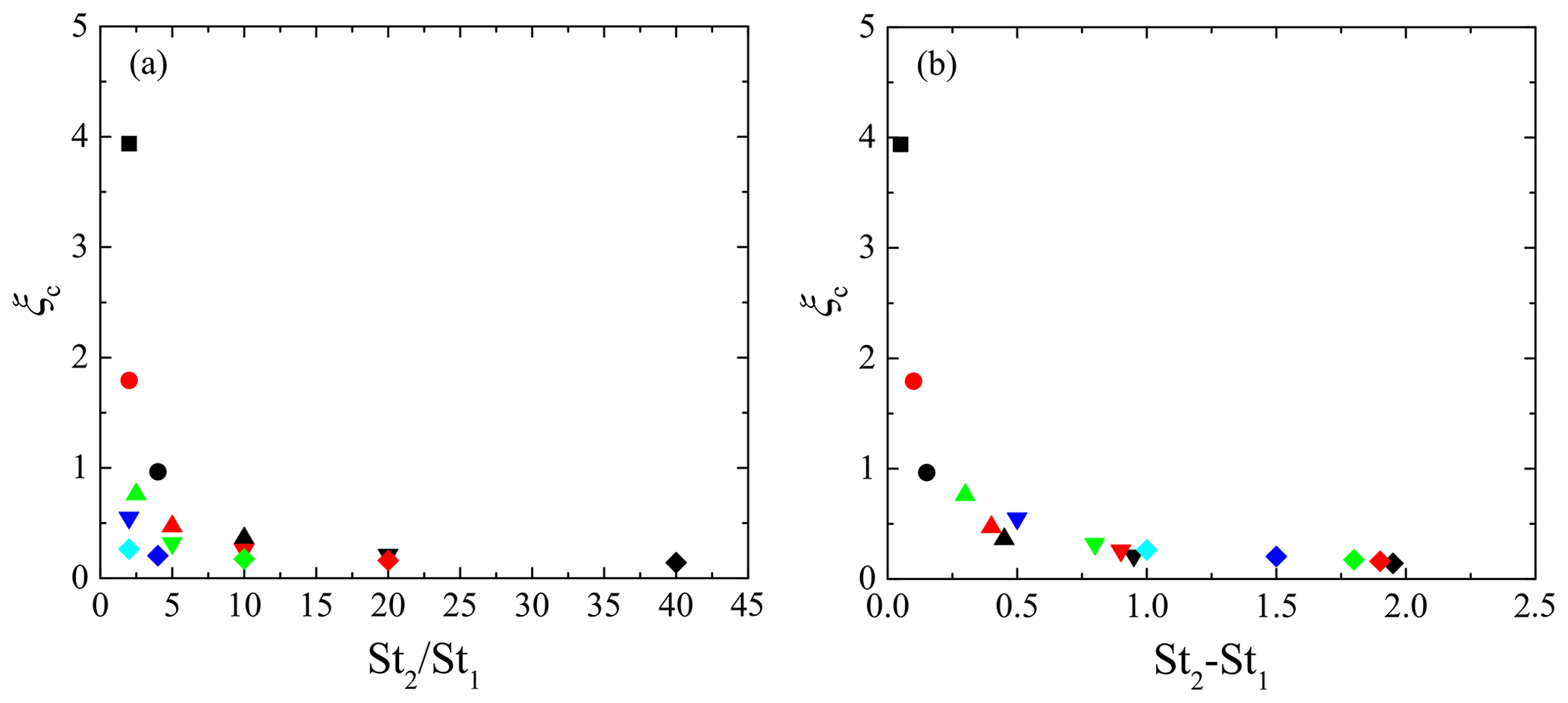
where ξc is the critical wave number normalized by the Kolmogorov scale, given by a function of St1 and St2. In this study, the critical wave number was obtained by finding the best-fitting exponential curve to the coherence for each combination of Stokes numbers. Figure 4 shows the critical wave numbers ξc for all combinations of St1 and St2, where St2>St1. ξc for the same St1 increases as St2 decreases, whereas ξc for the same St2 increases as St1 increases. This indicates that ξc increases as St1 and St2 becomes closer to each other. It should be noted that several studies discuss the spatial correlation of bidisperse clustering particles. For example, Zhou et al. (2001) developed the radial distribution function (RDF) model at the separation length of the Kolmogorov scale. They reported that the correlation coefficient of the bidisperse RDF obtained by their DNS is explained well by the ratio of two Stokes numbers. Chun et al. (2005) also discussed the bidisperse RDF of clustering particles. The result of their perturbation expansion analysis indicated that the bidisperse RDF becomes constant at separation lengths sufficiently smaller than the crossover length, lc, which is proportional to the Stokes number difference. As the cross spectrum of number density fluctuations is a Fourier transform of the bidisperse RDF, the Stokes number ratio, St2∕St1, and the Stokes number difference, St2–St1, are candidates for the dominant parameter for ξc. Figure 5 shows ξc plots against St2∕St1 and St2–St1. These figures clearly indicate that the Stokes number dependence of ξc is explained better by St2–St1 than St2∕St1. This would be because both the critical wave number ξc and crossover length lc represent the critical scale of the spatial correlation between the clusters for different Stokes numbers; i.e., the cluster locations are less correlated on a scale smaller than the critical scale. Based on this insight, we estimate that the critical wave number ξc is inversely proportional to the crossover length lc. Figure 6 shows ξc against the inverse of the Stokes number difference, which is generally expressed as . This figure confirms that ξc is approximately proportional to ; the least square fitting gives
This implies that ξc is closely related to the inverse of lc∕lη because the crossover length of Chun et al. (2005) is approximately based on their DNS data. It should be noted that the analytical results of Chun et al. (2005) are valid for St≪1. Thus, the deviation of ξc from the linear curve is due to the higher-order response of particle motions to the turbulent flow. However, Fig. 6 confirms that the Stokes number difference is the dominant parameter for ξc, at least for St≤2.0.
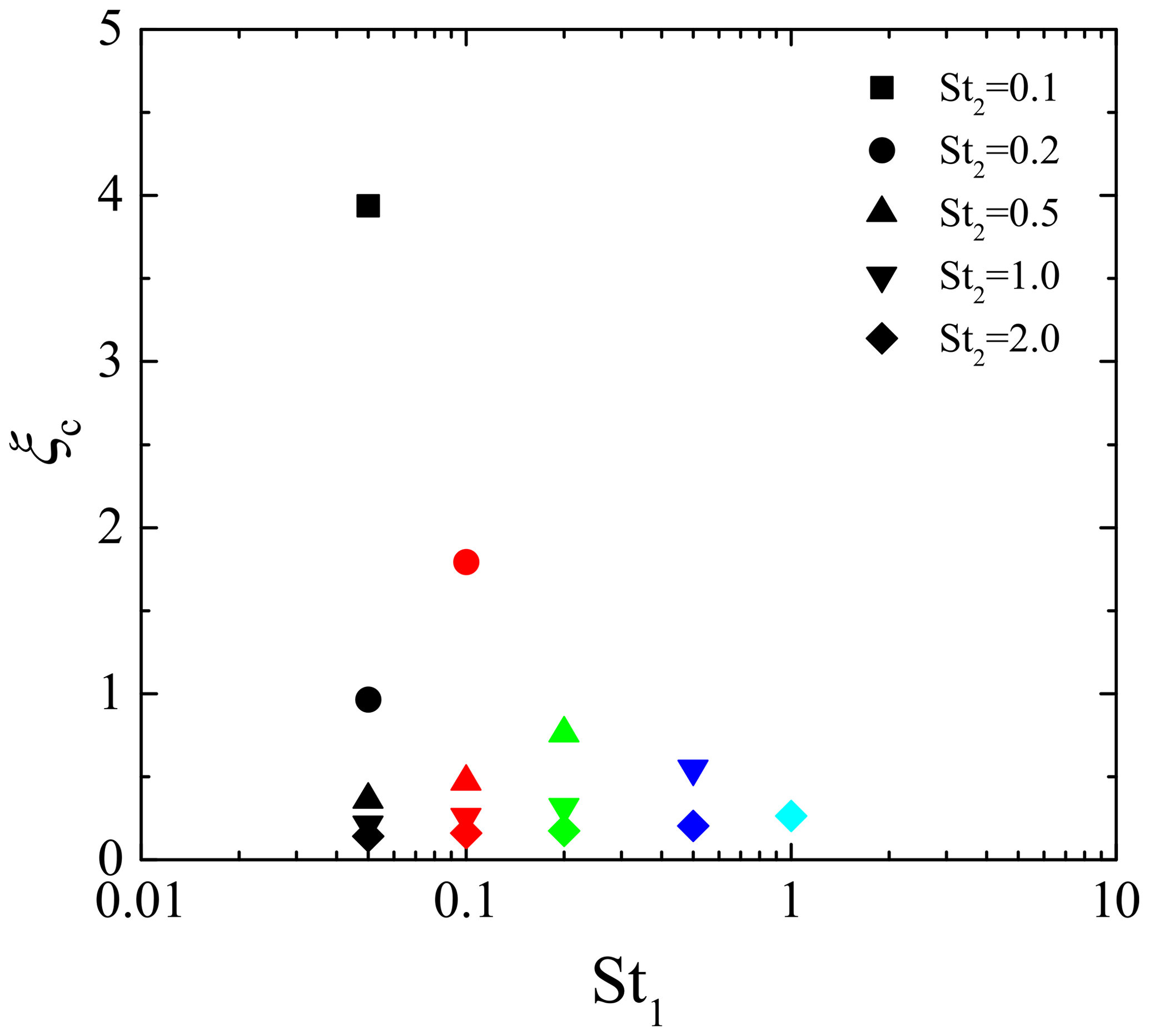
Figure 4Critical wave number ξc for a combination of Stokes numbers, St1 and St2. The symbol color and type indicate the combination of Stokes numbers. The black, red, green, blue, and light blue symbols are St1=0.05, 0.1, 0.2, 0.5, and 1.0, respectively. The square, circle, triangle, inverse triangle, and diamond symbols are St2=0.1, 0.2, 0.5, 1.0, and 2.0.
4.2 Modeling the influence of polydisperse clustering droplets on radar reflectivity factor
According to the above discussion, we can estimate the increase in the radar reflectivity factor due to turbulent clustering of polydisperse droplets in Eq. (9), provided that qr(rp) and 〈np〉 are given. That is, the normalized cross spectrum is given by
Here, we assume that the cross spectrum is a positive real number. The coherence is estimated using Eqs. (31) and (32). The parameterization for was proposed by Matsuda et al. (2014). The model equation is given by
where c1, c2, α, β, and γ are the model parameters given by the functions of St as follows:
Matsuda et al. (2014) confirmed that this parameterization is reliable for St≤2.0: in this range, the error of the parameterization is smaller than 1 dB.
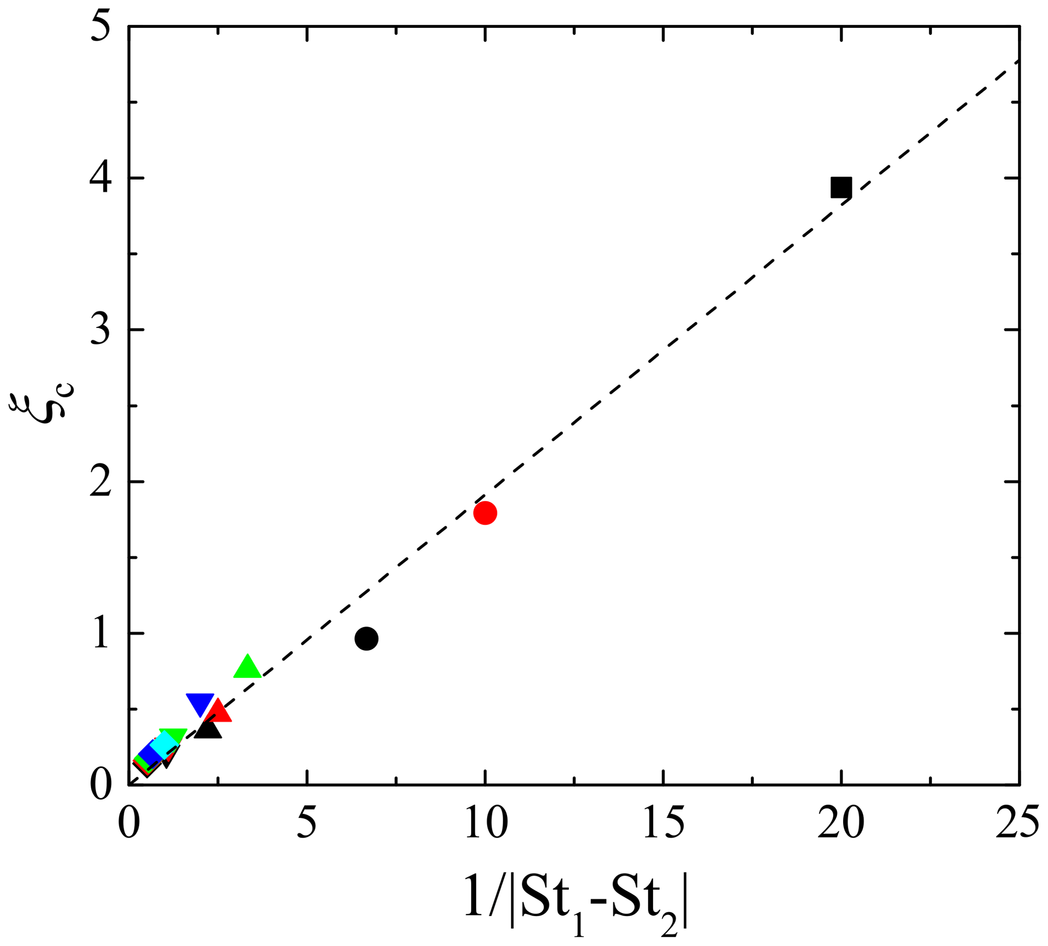
Figure 6Critical wave number ξc against the inverse of Stokes number difference. The dashed line is the best-fitting curve to the ξc data. Other notations are as in Fig. 4.
In order to evaluate the reliability of the proposed cross spectrum model, the -weighted power spectrum Er3np(k) for the droplet size distribution of CUMA has been estimated using the proposed cross spectrum model and compared with the spectrum obtained from the DNS data for the cases of CUMA_eps100, CUMA_eps400, and CUMA_eps1000. Figure 7a shows the -weighted power spectrum, which is normalized as
where is given by . The dashed lines show predicted using the proposed parameterization including Eq. (31), while the dashed-dotted lines show those predicted by assuming perfect coherence; i.e., . The parameterization with overestimates at large wave numbers and the difference becomes larger as ϵ becomes larger. This indicates that the influence of the weak spatial correlation of cluster locations between different Stokes numbers is not negligible for predicting the spectrum for large wave numbers, and the assumption of can be applied only for predicting for small wave numbers (). On the other hand, values predicted by the parameterization using Eq. (31) show good agreement with those obtained by the DNS data for overall wave numbers. The error level of the parameterization using Eq. (31) is evaluated by the rms error erms in units of decibels. erms is defined as
where ξ′ is defined as and superscript dB denotes a value in units of decibels. erms was calculated for the wave number range relevant to radar observations; i.e., . erms for the cases of CUMA_eps100, CUMA_eps400, and CUMA_eps1000 are 1.41, 0.152, and 0.251 dB, respectively. Because the error level of 1 dB is unavoidable for radar observations (Bringi et al., 1990; Carey et al., 2000), erms values for CUMA_eps400 and CUMA_eps1000 are negligibly small. erms for CUMA_eps100 is slightly larger than the threshold, but this is caused by the error of calculating the reference spectrum based on the DNS data at ξ>2. We confirm that, for CUMA_eps100, erms evaluated at the range of is smaller than 1 dB. Thus, the Stokes number dependence of the cross spectrum in the absence of gravity is appropriately modeled to predict the influence of turbulent clustering to a sufficient accuracy.

Figure 7Comparisons of -weighted power spectrum obtained from DNS data and estimated by the proposed cross spectrum model for the cases of (a) g=0.0 and (b) 9.8 m s−2.
4.3 Influence of gravitational settling on cross spectrum
The parameterization summarized in the previous subsection was obtained under the condition without gravitational droplet settling. The settling influence for the monodispersed cases was discussed by Matsuda et al. (2014, 2017). The large gravitational settling can modulate , and that can be a cause of the significant difference in the radar reflectivity factor. However, the influence on is insignificant for Sv<3 (Matsuda et al., 2014).
For the cases of polydisperse particles, the settling influence on the coherence term must be considered as well as the influence on in Eq. (33). Ayala et al. (2008a) and Lu et al. (2010) reported that gravitational settling enlarges the crossover length of the bidisperse RDF. Lu et al. (2010) extended the perturbation expansion analysis of Chun et al. (2005) and presented the formulation for the crossover length in the presence of gravity, which is
where CChun is the coefficient derived by Chun et al. (2005), a0 is the ratio of the acceleration variance 〈a2〉 to the square of the Kolmogorov acceleration , τa is the acceleration correlation timescale, and τg is the correlation timescale for gravitational settling particles. Chun et al. (2005) obtained the values of CChun≈5.0 and a0≈1.545 based on their DNS results. Lu et al. (2010) further assumed Sv≲1 so that τg is simply given by . The crossover length lc of Eq. (38) becomes equivalent to that of Chun et al. (2005) when gravitational settling is negligibly small, whereas the gravity effect is dominant for the cases of Fr<0.47, which often appears in cloud turbulence. Thus, in this study, we modify Eq. (32) to include the settling influence on the coherence . Since ξc is inversely proportional to lc∕lη, we propose the following correction based on Eq. (38):
Note that this study also adopts the value of a0 obtained by Chun et al. (2005).
The reliability of the modified parameterization for the case with gravitational settling has been evaluated in the same way as the previous subsection. Figure 7b shows for the case with gravitational settling. values at large wave numbers are smaller than those for the case without gravitational settling, and the difference from the parameterization with is larger, indicating that the coherence model is more important than the case without gravitational settling. It is also confirmed that values predicted by the proposed parameterization show good agreement with those of the DNS results for the case with gravitational settling. erms evaluated at the range of are 0.93 and 0.31 dB for the cases of CUMA_eps400 and CUMA_eps1000, respectively, and that for CUMA_eps100 at the range of is 0.26 dB. Thus, erms remains smaller than 1 dB, even for the case with gravitational settling. These results indicate that the proposed parameterization can predict the influence of turbulent clustering for polydisperse droplets considering the gravity effect to a sufficient accuracy. For the CUMA cases in Fig. 7b, Sv for the modal radius is smaller than unity. For the cases of Sv>O(1), the proposed parameterization would become less reliable. To improve the parameterization, it is necessary to consider an anisotropic clustering structure of settling inertial particles. Inertial particles with a large settling velocity form anisotropic clusters, which are vertically elongated and horizontally confined (Bec et al., 2014; Ireland et al., 2016; Matsuda et al., 2017). When the clustering structure is anisotropic, the influence on the radar reflectivity factor theoretically depends on the direction of microwave propagation.
5.1 Cloud simulation data
We have applied the proposed model to the high-resolution cloud-simulation data of Onishi and Takahashi (2012) to investigate the influence of turbulent clustering on radar observations. They used the Multi-Scale Simulator for the Geoenvironment (MSSG), which is a multi-scale atmosphere–ocean coupled model developed by the Japan Agency for Marine-Earth Science and Technology. The atmospheric component of MSSG (MSSG-A) solves nonhydrostatic equations and predicts three wind components, air density, and pressure, as well as water substance. Finite-difference schemes are used for calculating spatial derivatives. Turbulent diffusion is calculated using the static Smagorinsky model. Onishi and Takahashi (2012) used a spectral-bin scheme for liquid water to explicitly account for the droplet size distributions. The spectral bin scheme predicts the mass distribution function G(y), which is given by
where y=ln rp, and m(rp) is the mass of droplets with a radius of rp. The mass coordinate m and logarithmic coordinate y are discretized as
where , and s is a constant; s=1 was used. The number of bins was 33. The representative radius of the first bin, rp1, was 3 µm; thus, the representative radius of the 33rd bin (the largest droplet class) was rp33=4.9 mm. The prognostic variable for liquid water is the water mass content, Mk, which is defined as ; i.e., 33 transport equations for Mk were solved in this simulation. The activation process of cloud condensation nuclei (CCN) was considered based on Twomey's relationship between the number of activated CCN and the saturation ratio (Twomey, 1959). The activated droplets were added to the bins using the prescribed spectrum method (Soong, 1974). Details of the model configuration are described in Onishi and Takahashi (2012). The model settings and computational conditions were based on the protocol of the RICO model intercomparison project (van Zanten et al., 2006, http://www.knmi.nl/samenw/rico/, last access: 6 February 2019). The protocol is based on the rain in cumulus over the ocean (RICO) field campaign. The domain size is km. The resolution setting of the original RICO protocol is 128×128 points in the horizontal directions and 100 points in the vertical direction; i.e., m and Δz=40 m. Onishi and Takahashi (2012) performed the cloud simulation for 24 h using the original resolution setting, then continued it for an additional hour using a higher-resolution setting, generating 512×512 points in the horizontal directions and 200 points in the vertical direction, giving grid spacings of m and Δz=20 m. This study used the temporal slice of cloud simulation data at a higher resolution.
5.2 Computational method for radar reflectivity factor
The radar reflectivity factor Z, including the influence of particulate and clear-air Bragg scatterings, is given by
where ZPB is the particulate Bragg-scattering part of Z in Eq. (9), and ZCB is an additional term reflecting clear-air Bragg scattering. In real clouds, ZPB is caused by droplet number density fluctuations due to turbulent droplet clustering and turbulent entrainment of environmental clear air. Er3np(k) for these factors is given by (Matsuda et al., 2014), where and are the power spectra for turbulent clustering and entrainment. Note that the correlation term between the cloud water fluctuations due to these factors is negligibly small because the scales of the clustering and entrainment sources are typically separated. Thus, ZPB is also given by the linear combination; i.e., , where and .
The spectrum was calculated using Eq. (10) and the parameterization proposed in the previous section. To determine the Stokes number for each droplet size, the energy dissipation rate ϵ of the cloud simulation data was calculated based on the Smagorinsky model; i.e.,
where Cs is the Smagorinsky constant (Cs=0.173 in this study), Δs the representative grid spacing given by , and the strain rate tensor, which is given by , where is the air velocity in the resolved scale.
The spectrum was calculated using the well-known scalar concentration spectrum. Erkelens et al. (2001) estimated this contribution based on the power law in the inertial-convective range of the spectrum. In this study, the −1 power law in the viscous-convective range (klη<0.1) is also considered, since the diffusive coefficient Dnp for droplet number density is much smaller than ν. is approximately given by (Hill, 1978)
where χr3np is the scalar dissipation rate for , Cc is the Obukhov–Corrsin constant (Cc=0.67) (Sreenivasan, 1996; Goto and Kida, 1999), Cb is the Batchelor constant (Cb=3.7) (Grant et al., 1968; Goto and Kida, 1999), and γ′ is the model parameter ().
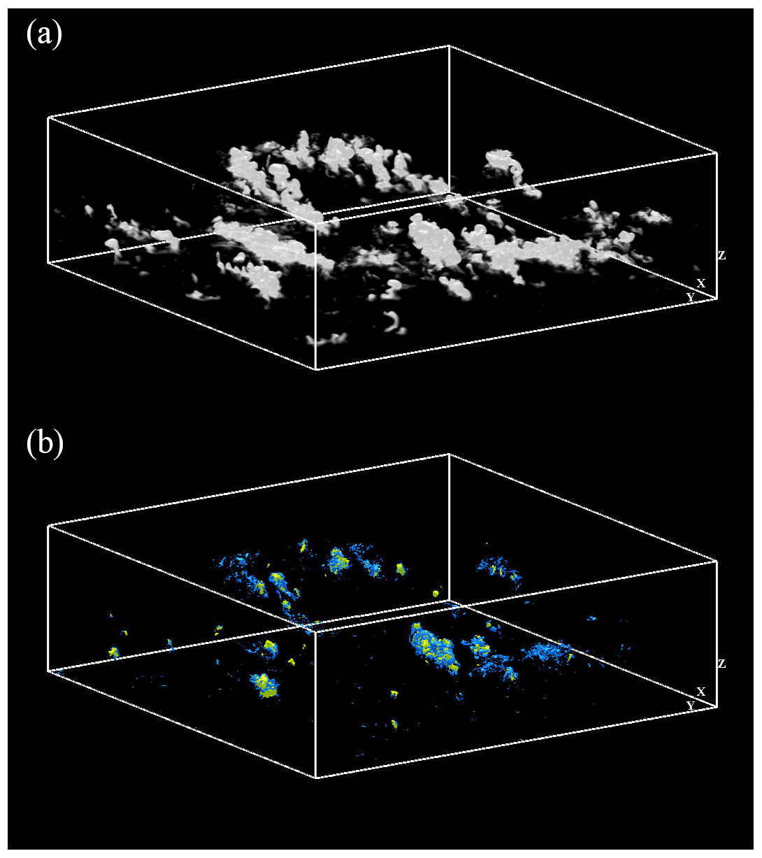
Figure 8Three-dimensional visualization of cloud simulation data: (a) volume rendering of optical depth and (b) isosurfaces of (blue) the energy dissipation rate ϵ=100 cm2 s−3 and (yellow) the vertical velocity u3=3 m s−1.
The contribution of clear-air Bragg scattering was calculated by
where En(k) is the power spectrum of refractive index fluctuations. The refractive index nref is given approximately by (Balsley and Gage, 1980)
where p and e are the atmospheric pressure and partial pressure of water vapor in hPa, and T is the absolute temperature. The contribution of free electrons was omitted because it is negligibly small in the troposphere. The power spectrum En(k) is given by the scalar concentration spectrum for Pr<1 (Pao, 1964), where (D is the scalar diffusive coefficient) is the Prandtl number:
where χn is the scalar dissipation rate for nref. In this study, the Prandtl number of refractive index was set to 0.7.
The scalar dissipation rates for and nref were calculated in the same way. That is, the dissipation rate of an arbitrary scalar θ is given by
where νt is the eddy kinematic viscosity, Sct is the turbulent Schmidt number, and is the scalar value in the resolved scale. νt was calculated by using the Smagorinsky model; i.e., , and Sct was set to 0.4 (Moin et al., 1991).
5.3 Results and discussion
Figure 8a shows the three-dimensional visualization of liquid water. The optical thickness of each grid cell, τΔ, is visualized by volume rendering to mimic human-eye observations of clouds. Here, the optical thickness is defined by , where Qext is the extinction efficiency for Mie scattering (Qext=2.0 in this study), and is given by . Note that the optical transmittance of cloud volume is approximately equal to 1−τΔ when τΔ is sufficiently smaller than unity. Figure 8b shows the isosurfaces of the energy dissipation rate ϵ and the vertical velocity u3. The locations of upward flows correspond to the locations of clouds and large ϵ regions are observed around the upward flows. This indicates that strong turbulence is generated by entrainment motions due to updrafts.

Figure 9Liquid water content (LWC), energy dissipation rate ϵ, and radar reflectivity factors for S-band microwaves in the vertical cross section: (a) LWC in a logarithmic scale (i.e., log 10LWC – g m−3), (b) ϵ (m2 s−3), (c) ZdB (dBZ), (d) (dB), and (e) (dBZ). The solid lines in (c)–(e) indicate the isoline of dBZ.
This study focused on a vertical cross section that slices the cumulus cloud with the largest upward velocity. Figure 9 shows the liquid water content (LWC) in a logarithmic scale, the energy dissipation rate ϵ, the radar reflectivity factor ZdB, the increase of ZdB due to particulate Bragg scattering, and particulate Bragg scattering due to turbulent clustering in the cross section. The microwave frequency was set to fm=2.8 GHz, which is the representative frequency of S-band radars. The radar reflectivity factor is shown in units of decibels, which is defined as ZdB (dBZ)=10log 10Z (mm6 m−3). Large values of ZdB are observed inside and below the clouds. The strong echo below the clouds reflects drizzling regions, where the LWC is smaller than that inside the clouds but the strong echo returns from the drizzling droplets because Zincoh is proportional to . The radar echo on the outside of the isoline of dBZ is caused by clear-air Bragg scattering, i.e., ZCB. The radar echo layer at the height from 2.2 to 2.5 km is caused by ZCB due to a large humidity gap in the inversion layer.
Figure 9c does not show a clear sign of the mantle echo reported by Knight and Miller (1998). Knight and Miller (1998) reported that the predominant mantle echo is observed on dry days, while it is poorly observed on the most humid day. Our result is in accord with this report, as the relative humidity of the environmental air is above 80 % at heights below about 2.2 km in our cloud simulation data. A possible cause of the mantle echo is particulate Bragg scattering due to turbulent entrainment (i.e., ZPBe) because the large-scale cloud water inhomogeneity at cloud edges produces small-scale fluctuations due to the turbulent cascade (Erkelens et al., 2001). The influence of turbulent entrainment on ZdB turned out to be, however, negligibly small. That is, the fluctuations caused by the large-scale inhomogeneity were not significantly large at the scale of the half wavelength in the present simulation.
In Fig. 9d, the increase due to particulate Bragg scattering, , is significant at the near-top of the clouds. The maximum difference is larger than 5 dB. In order to discuss the reason for the strong clustering influence at the near-top of the clouds, the raw value of is plotted in Fig. 9e. is larger than −10 dBZ inside the turbulent cloud region, where the LWC is larger than 0.1 g m−3, and the energy dissipation rate ϵ is intermittently larger than 100 cm2 s−3. Large values of are shown at the near-top inside this cloud region. We have confirmed that the droplet size in this cloud region was almost homogeneous: the volume-averaged droplet radius ranged within 7 to 11 µm. As a result, large values of the Stokes number (up to 0.05) distributed intermittently corresponding to the distribution of ϵ. The main factor of the height dependence of is the LWC, which is larger than 1 g m−3 at the near-top of the clouds. Note that ZPBc is proportional to square of the LWC as Eqs. (9) and (36) implies . Thus, the significant influence of turbulent clustering is caused by sufficiently large values of the energy dissipation rate and the LWC.
This study has investigated the influence of microscale turbulent clustering of polydisperse cloud droplets on the radar reflectivity factor. Firstly, the theoretical solution for particulate Bragg scattering for polydisperse droplets has been obtained considering the droplet size distribution in the measurement volume and the droplet size dependence of turbulent clustering. The obtained formula shows that the particulate Bragg-scattering part of the radar reflectivity factor is given by a double integral function including the cross spectrum of number density fluctuations for bidisperse droplets. Secondly, the wave number and Stokes number dependence of the cross spectrum has been investigated using the turbulent droplet clustering data obtained from a direct numerical simulation (DNS) of particle-laden homogeneous isotropic turbulence without gravitational settling. The result shows that the cross spectrum for a combination of Stokes numbers, St1 and St2, has values between the power spectra for St1 and St2 at small wave numbers, whereas the spectrum decreases more rapidly than the power spectra as the wave number increases. This decreasing trend is related to the scale dependence of the spatial correlation of cluster locations between two different Stokes numbers. The coherence of the cross spectrum is close to unity for small wave numbers and decreases almost exponentially with increasing wave number. This is qualitatively consistent with the visualization results, in which the clustering locations for different Stokes numbers are almost the same on large scales, whereas a discrepancy in clustering locations is observed at small scales. It is also confirmed that the decreasing trend of the coherence is strongly dependent on the combination of Stokes numbers.
In order to develop a cross spectrum model for estimating the clustering influence on the radar reflectivity factor, we have proposed an exponential model for the wave number dependence of the coherence and introduced the critical wave number (i.e., the decay constant for the model) to consider the dependence of the coherence on the Stokes number combination. The coherence data for all combinations of six Stokes numbers ranging from 0.05 to 2.0 reveal that the critical wave number is inversely proportional to the Stokes number difference, . This implies that the critical wave number is inversely proportional to the crossover length for the bidisperse radial distribution function (RDF). The proposed coherence model enables us to estimate the cross spectrum for arbitrary combinations of Stokes numbers using the power spectrum model proposed by Matsuda et al. (2014). Comparison of the model estimate with the DNS results for a typical droplet size distribution in cumulus clouds confirms the reliability of the Stokes number dependence of the proposed model.
The proposed model has been further extended for the case with gravitational settling. We have assumed Sv≲1, where Sv is the settling parameter, and modified the parameterization for the critical wave number based on the analytical equation for the crossover length considering the settling influence (Lu et al., 2010). The -weighted power spectrum estimated by the modified model shows a good agreement with that obtained by the DNS data considering the droplet size distribution in cumulus clouds and gravitational settling, indicating that the proposed model can estimate the clustering influence on the radar reflectivity factor to a sufficient accuracy.
Finally, the proposed model has been applied to high-resolution cloud-simulation data of Onishi and Takahashi (2012). The data were obtained using the Multi-Scale Simulator for the Geoenvironment (MSSG), which is a multi-scale nonhydrostatic atmosphere–ocean coupled model. The cloud and rain droplet size distribution was explicitly calculated at each grid using a spectral-bin cloud microphysics scheme. The radar reflectivity factor has been calculated considering particulate Bragg scattering due to turbulent clustering and turbulent entrainment as well as clear-air Bragg scattering caused by temperature and humidity fluctuations. The result shows that the influence of turbulent entrainment is negligibly small in our case, whereas the influence of turbulent clustering can be significant inside turbulent clouds. The large influence is observed at the near-top of the clouds, where the liquid water content (LWC) and the energy dissipation rate are sufficiently large.
Access to the simulation and analysis results can be granted upon request under a collaborative framework with JAMSTEC.
KM designed the study, conducted the DNSs, developed the parameterization based n the DNS data, and analyzed the cloud simulation data. RO developed the DNS program, and provided the cloud simulation data. Both authors contributed to the discussion, interpretation of the results, and to writing the paper.
The authors declare that they have no conflict of interest.
This research was supported by JSPS KAKENHI grant number JP17K14598. The
numerical simulations presented were carried out on the Earth Simulator
supercomputer system of the Japan Agency for Marine-Earth Science and
Technology (JAMSTEC).
Edited by: Graham Feingold
Reviewed by: two anonymous referees
Ayala, O., Rosa, B., and Wang, L.-P.: Effects of turbulence on the geometric collision rate of sedimenting droplets. Part 2. Theory and parameterization, New J. Phys., 10, 075016, https://doi.org/10.1088/1367-2630/10/7/075016, 2008a. a, b
Ayala, O., Rosa, B., Wang, L.-P., and Grabowski, W.: Effects of turbulence on the geometric collision rate of sedimenting droplets. Part 1. Results from direct numerical simulation, New J. Phys., 10, 075015, https://doi.org/10.1088/1367-2630/10/7/075015, 2008b. a
Balsley, B. and Gage, K.: The MST Radar Technique: Potential for Middle Atmospheric Studies, Pure Appl. Geophys., 118, 452–493, 1980. a
Bec, J., Homann, H., and Ray, S.: Gravity-Driven Enhancement of Heavy Particle Clustering in Turbulent Flow, Phys. Rev. Lett., 112, 184501, https://doi.org/10.1103/PhysRevLett.112.184501, 2014. a, b
Bohren, C. and Huffman, D.: Absorption and Scattering of Light by Small Particles, Wiley, 1983. a
Bringi, V., Chandrasekar, V., Balakrishnan, N., and Zrnić, D.: An examination of propagation effects in rainfall on radar measurements at microwave frequencies, J. Atmos. Ocean. Tech., 7, 829–840, 1990. a
Carey, L., Rutledge, S., Ahijevych, D., and Keenan, T.: Correcting Propagation Effects in C-Band Polarimetric Radar Observations of Tropical Convection Using Differential Propagation Phase, J. Atmos. Sci., 39, 1405–1433, 2000. a
Chen, L., Goto, S., and Vassilicos, J.: Turbulent clustering of stagnation points and inertial particles, J. Fluid Mech., 553, 143–154, 2006. a
Chun, J., Koch, D., Rani, S., Ahluwalia, A., and Collins, L.: Clustering of aerosol particles in isotropic turbulence, J. Fluid Mech., 536, 219–251, 2005. a, b, c, d, e, f, g, h
Dombrovsky, L. and Zaichik, L.: An effect of turbulent clustering on scattering of microwave radiation by small particles in the atmosphere, J. Quant. Spectrosc. Ra., 111, 234–242, 2010. a
Erkelens, J., Venema, V., Russchenberg, H., and Ligthart, L.: Coherent Scattering of Microwave by Particles: Evidence from Clouds and Smoke, J. Atmos. Sci., 58, 1091–1102, 2001. a, b, c, d
Gossard, E. and Strauch, R.: Radar Observation of Clear Air and Clouds, in: vol. 14 of Developments in Atmospheric Science, Elsevir, New York, 1983. a, b, c, d, e
Goto, S. and Kida, S.: Passive scalar spectrum in isotropic turbulence: Prediction by the Lagrangian direct-interaction approximation, Phys. Fluids, 11, 1936–1952, 1999. a, b
Grabowski, W. and Vaillancourt, P.: Comments on “Preferential Concentration of Cloud Droplets by Turbulence: Effects on the Early Evolution of Cumulus Cloud Droplet Spectra”, J. Atmos. Sci., 56, 1433–1436, 1999. a
Grant, H., Hughes, B., Vogel, W., and Moilliet, A.: The spectrum of temperature fluctuations in turbulent flow, J. Fluid Mech., 34, 423–442, 1968. a
Hess, M., Koepke, P., and Schult, I.: Optical Properties of Aerosols and Clouds: The Software Package OPAC, B. Am. Meteorol. Soc., 79, 831–844, 1998. a
Hill, R.: Models of the scalar spectrum for turbulent advection, J. Fluid Mech., 88, 541–562, 1978. a
Hirt, C. and Cook, J.: Calculating three-dimensional flow around structures, J. Comput. Phys., 10, 324–340, 1972. a
Ireland, P., Bragg, A., and Collins, L.: The effect of Reynolds number on inertial particle dynamics in isotropic turbulence. Part 2. Simulations with gravitational effects, J. Fluid Mech., 796, 659–711, 2016. a, b
Knight, C. and Miller, L.: Early radar echoes from small, warm cumulus: Bragg and hydrometeor scattering, J. Atmos. Sci., 55, 2974–2992, 1998. a, b, c, d
Kostinski, A. and Jameson, A.: On the spatial distribution of cloud particles, J. Atmos. Sci., 57, 901–915, 2000. a, b
Lu, J., Nordslek, H., and Shaw, R.: Clustering of settling charged particles in turbulence: theory and experiments, New J. Phys., 12, 123030, https://doi.org/10.1088/1367-2630/12/12/123030, 2010. a, b, c, d
Matsuda, K., Onishi, R., Hirahara, M., Kurose, R., Takahashi, K., and Komori, S.: Influence of microscale turbulent droplet clustering on radar cloud observations, J. Atmos. Sci., 71, 3569–3582, 2014. a, b, c, d, e, f, g, h, i, j, k
Matsuda, K., Onishi, R., and Takahashi, K.: Influence of gravitational settling on turbulent droplet clustering and radar reflectivity factor, Flow Turb. Combust., 98, 327–340, 2017. a, b
Maxey, M.: The gravitational settling of aerosol particles in homogeneous turbulence and random flow fields, J. Fluid Mech., 174, 441–465, 1987. a
Moin, P., Squires, K., Cabot, W., and Lee, S.: A dynamic subgridscale model for compressible turbulence and scalar transport, Phys. Fluids A, 3, 2746–2757, 1991. a
Morinishi, Y., Lundm, T., Vasilyev, O., and Moin, P.: Fully conservative higher order finite difference schemes for incompressible flow, J. Comput. Phys., 143, 90–124, 1998. a
Onishi, R. and Takahashi, K.: A Warm-Bin–Cold-Bulk Cloud Microphysical Model, J. Atmos. Sci., 69, 1474–1497, 2012. a, b, c, d, e
Onishi, R. and Vassilicos, J.: Collision Statistics of Inertial Particles in Two-Dimensional Homogeneous Isotropic Turbulence with an Inverse Cascade, J. Fluid Mech., 745, 279–299, 2014. a
Onishi, R., Takahashi, K., and Komori, S.: Influence of gravity on collisions of monodispersed droplets in homogeneous isotropic turbulence, Phys. Fluids, 21, 125108, https://doi.org/10.1063/1.3276906, 2009. a
Onishi, R., Baba, Y., and Takahashi, K.: Large-Scale Forcing with Less Communication in Finite-Difference Simulations of Steady Isotropic Turbulence, J. Comput. Phys., 230, 4088–4099, 2011. a
Pao, Y.: Statistical Behavior of a Turbulent Multicomponent Mixture with First-Order Reactions, AIAA J., 2, 1550–1559, 1964. a
Pinsky, M., Khain, A., and Krugliak, H.: Collision of Cloud Droplets in a Turbulent Flow. Part V: Application of Detailed Tables of Turbulent Collision Rate Enhancement to Simulation of Droplet Spectra Evolution, J. Atmos. Sci., 65, 357–374, 2008. a
Reade, W. and Collins, L.: Effect of preferential concentration on turbulent collision rates, Phys. Fluids, 12, 2530, https://doi.org/10.1063/1.1288515, 2000. a
Rogers, R. and Brown, W.: Radar Observations of a Major Industrial Fire, B. Am. Meteorol. Soc., 78, 803–814, 1997. a
Soong, S.-T.: Numerical simulation of warm rain development in an axisymmetric cloud model, J. Atmos. Sci., 31, 1262–1285, 1974. a
Squires, K. and Eaton, J.: Preferential concentration of particles by turbulence, Phys. Fluids A, 3, 1169–1178, 1991. a
Sreenivasan, K.: The passive scalar spectrum and the Obukhov–Corrsin constant, Phys. Fluids, 8, 189–196, 1996. a
Sundaram, S. and Collins, L.: Collision statistics in an isotropic particle-laden turbulent suspension. Part 1. Direct numerical simulations, J. Fluid Mech., 335, 75–109, 1997. a
Twomey, S.: The nuclei of natural cloud formation. Part II: The supersaturation in natural clouds and the variation of cloud droplets concentrations, Geofis. Pura Appl., 43, 243–249, 1959. a
van Zanten, M., Nuijens, L., and Siebesma, A.: Precipitating Shallow Cumulus Case1, available at: http://www.knmi.nl/samenw/rico/ (last access: 6 February 2019), 2006. a
Wang, L. and Maxey, M.: Settling velocity and concentration distribution of heavy particles in homogeneous isotropic turbulence, J. Fluid Mach., 256, 27–68, 1993. a, b
Wang, L., Rosa, B., Gao, H., He, G., and Jin, G.: Turbulent collision of inertial particles: Point-particle based, hybrid simulations and beyond, Int. J. Multiphase Flow, 35, 854–867, 2009. a
Zhou, Y., Wexler, A., and Wang, L.: Modelling turbulent collision of bidisperse inertial particles, J. Fluid Mech., 433, 77–104, 2001. a