the Creative Commons Attribution 4.0 License.
the Creative Commons Attribution 4.0 License.
 | 16 Dec 2019
The regional temperature implications of strong air quality measures
Borgar Aamaas
Terje Koren Berntsen
Bjørn Hallvard Samset
Anthropogenic emissions of short-lived climate forcers (SLCFs) affect both air quality and climate. How much regional temperatures are affected by ambitious SLCF emission mitigation policies is, however, still uncertain. We investigate the potential temperature implications of stringent air quality policies by applying matrices of regional temperature responses to new pathways for future anthropogenic emissions of aerosols, methane (CH4), and other short-lived gases. These measures have only a minor impact on CO2 emissions. Two main options are explored, one with climate optimal reductions (i.e., constructed to yield a maximum global cooling) and one with the maximum technically feasible reductions. The temperature response is calculated for four latitude response bands (90–28∘ S, 28∘ S–28∘ N, 28–60∘ N, and 60–90∘ N) by using existing absolute regional temperature change potential (ARTP) values for four emission regions: Europe, East Asia, shipping, and the rest of the world. By 2050, we find that global surface temperature can be reduced by ∘C with climate-optimal mitigation of SLCFs relative to a baseline scenario and as much as −0.7 ∘C in the Arctic. Cutting CH4 and black carbon (BC) emissions contributes the most. The net global cooling could offset warming equal to approximately 15 years of current global CO2 emissions. On the other hand, mitigation of other SLCFs (e.g., SO2) leads to warming. If SLCFs are mitigated heavily, we find a net warming of about 0.1 ∘C, but when uncertainties are included a slight cooling is also possible. In the climate optimal scenario, the largest contributions to cooling come from the energy, domestic, waste, and transportation sectors. In the maximum technically feasible mitigation scenario, emission changes from the industry, energy, and shipping sectors will cause warming. Some measures, such as those in the agriculture waste burning, domestic, transport, and industry sectors, have large impacts on the Arctic, especially by cutting BC emissions in winter in areas near the Arctic.
- Article
(2737 KB) - Full-text XML
-
Supplement
(851 KB) - BibTeX
- EndNote


Poor air quality is an issue of global concern, with health and welfare impacts affecting billions of people (WHO, 2016; Dockery et al., 1993; Di et al., 2017). Additionally, many of the components that make up air pollution also lead to radiative forcing, impacting climate through scattering or absorbing solar radiation or by acting as greenhouse gases (Myhre et al., 2013b; von Schneidemesser et al., 2015). The net and individual climate impacts of present emissions of such short-lived climate forcers (SLCFs) have been extensively studied, but they are however still poorly constrained (Stohl et al., 2015; Aamaas et al., 2016; Myhre et al., 2017; Samset et al., 2018). The SLCFs considered here are black carbon (BC), organic carbon (OC), sulfur dioxide (SO2), nitrogen oxides (NOx), carbon monoxide (CO), volatile organic compounds (VOC), and methane (CH4). CH4, which is a greenhouse gas and a precursor of O3 and stratospheric water vapor, is the SLCF that gives the largest warming at current emission levels. BC (also known as soot) is a result of incomplete combustion that causes not only warming through absorption of sunlight and reduced albedo of contaminated snow and ice surfaces but also cooling, mainly by affecting clouds. Removing all anthropogenic BC emissions would cause a cooling of −0.05 ∘C according to Stohl et al. (2015). Several aerosols are cooling the climate through scattering solar radiation and altering the radiative properties of clouds, with sulfate aerosol formed from SO2 and ammonia (NH3) giving the largest cooling. Stohl et al. (2015) estimate that removing all anthropogenic emissions of SO2 would increase the global temperature by 0.69 ∘C. OC is another cooling aerosol, and a complete removal of anthropogenic OC emissions would lead to a warming of 0.13 ∘C (Stohl et al., 2015). The ozone precursors NOx, CO, and VOC produce tropospheric O3, which is a greenhouse gas. Emissions of these species will also impact the hydroxyl radical (OH) concentration, which impacts CH4. The impact of current emissions of these ozone precursors is small compared to the impact of current emissions of CH4 and SO2.
In the coming decades, mitigation of CO2 and other long-lived greenhouse gases (LLGHGs) is vital for the success of the goals in the Paris Agreement (UNEP, 2016). Concurrently, we expect large changes in SLCF emissions in response to air quality policies, additional to climate change mitigation efforts and due to co-emissions with LLGHGs. As some SLCFs cool the climate, others warm it, and some may do both at different times after emission; the exact mitigation pathways of SLCFs will be of importance for the near-term rate and magnitude of warming – both globally and regionally. While several studies have analyzed the impact on CO2 mitigation of SLCFs (e.g., Rogelj et al., 2014), our study does not consider CO2 emissions but investigates a set of air quality measures that mainly influence SLCF emissions.
Designing mitigation measures with both air quality and climate change in mind is however not straightforward, as warming SLCFs are often co-emitted with cooling SLCFs. Some authors have argued that a mitigation focus on SLCFs can be counterproductive, as this may lead to relaxing efforts on reducing CO2 emissions (Pierrehumbert, 2014; Shoemaker et al., 2013). However, if this is done in a consistent way, using emission metrics with appropriate time horizons, this can be avoided (Berntsen et al., 2010). Another argument against SLCF mitigation today is that the long-term cooling potential of emission reductions is limited and that delaying mitigation of SLCFs has only minor impact on temperature stabilization and peaking in the future (e.g., Pierrehumbert, 2014). However, SLCF mitigation is already occurring as part of air quality policy (Li et al., 2017) and is expected to continue in the coming decades regardless of the level of climate mitigation ambitions (Victor et al., 2015; Rao et al., 2017). Stohl et al. (2015) showed (applying the absolute regional temperature change potential (ARTP) methodology) that climate optimal reductions of SLCFs, i.e., the combination of measures which maximize temperature reduction, may lower the global temperature by 0.22 ∘C in 2041–2050, compared to a reference scenario. In comparison, a complete removal of anthropogenic emissions of black carbon (BC), organic carbon (OC), and SO2 (sulfate aerosol precursor) would induce a global mean surface heating of 0.5–1.1 ∘C, according to four recent climate models (Samset et al., 2018). Going beyond temperature and precipitation impacts, SLCF emission mitigation is also known to have multiple co-benefits and trade-offs with the UN Sustainable Development Goals (SDGs) (Haines et al., 2017). The co-benefits are generally larger than the trade-offs. Among the most well-known co-benefits, we find that SLCF mitigation will reduce air pollution and, hence, reduce premature deaths (SDG3), as well as reduce crop losses (SDG2).
Recently, Stohl et al. (2015) gave a general overview of the temperature reduction potential of SLCFs. That paper synthesized the work in the project ECLIPSE (Evaluating the Climate and Air Quality Impacts of Short-Lived Pollutants) (IIASA, 2016). The project designed realistic and effective mitigation scenarios for SLCFs and quantified their climate and air quality impacts. The work started with producing new emission inventories for the recent past and through 2050. Those emissions were applied in several advanced Earth system models (ESMs) and chemistry transport models (CTMs). The climate impacts were estimated with two different paths of research, where the first was to calculate radiative forcing (RF) and then produce emission metrics such as ARTP. The second path was for modeling transient climate responses with ESMs. Results from the first path were applied in an integrated assessment model to identify emission mitigation measures that are both beneficial for air quality and short-term climate impact. That study found that estimates on global temperature change are similar for the decade 2041–2050 by applying these two different paths. Further, the two different research paths partly agree on how much emission changes in CH4 versus emission changes of the other SLCFs are responsible for the temperature change. Our study utilizes several aspects of the ECLIPSE research, including emission inventories, mitigation pathways, and ARTP values. We explore the findings in Stohl et al. (2015) further for individual emission regions and emission sectors using updated data and methods, following pathways that focus on air quality concerns. Our focus is on the temperature effects of SLCFs; however, mitigation of these components can also help to achieve several of the Sustainable Development Goals (Shindell et al., 2017).
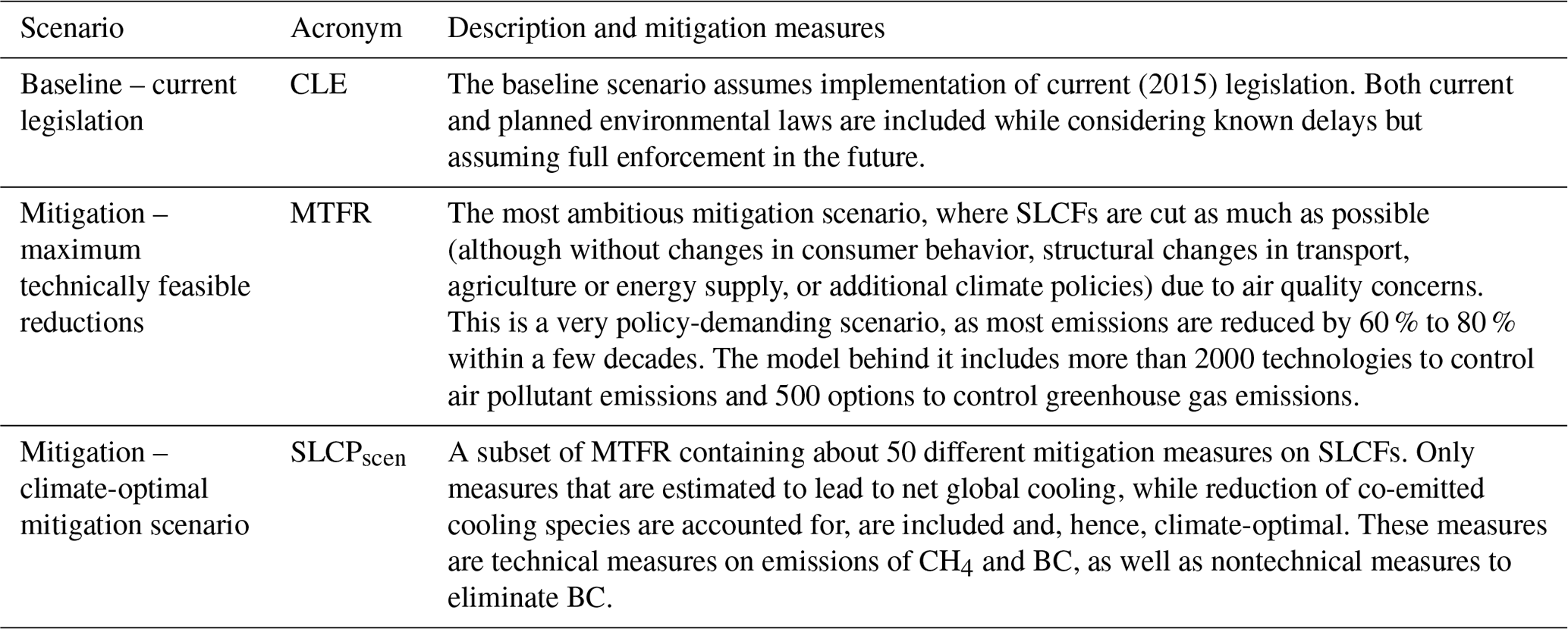
A detailed look into what sectors and regions contribute to the mitigation potential from SLCF reductions requires a comprehensive emission dataset. As part of the ECLIPSE project, emission inventories and scenarios for future emissions (for the period 1990–2050) of SLCFs were produced (Klimont et al., 2017, 2019). The scenarios describe three different futures with different mitigating ambitions (see Table 1): one baseline with current legislation (CLE), one with as much mitigation of SLCFs as possible (MTFR), and one which only include measures that lead to net global cooling (Stohl et al., 2015). The MTFR scenario is demanding, as emissions of SLCFs are cut by 60 % to 80 % within a few decades. However, similar trends have historically been seen for emissions of SO2 and NOx in Western Europe and North America (Amann et al., 2013; Rafaj et al., 2015). The third scenario can be seen as a subset of MTFR, as this climate-optimal mitigation scenario (SLCPscen) includes roughly 50 different mitigation measures on SLCFs from the MTFR catalogue of measures that avoid warming. The scenario name SLCPscen, based on the scenario name SLCP given by The International Institute for Applied Systems Analysis (IIASA), should not be mixed up with the term short-lived climate pollutant. Every selected measure gives a net cooling based on the global temperature change potential values for a time horizon of 20 years, given a linear ramp-up of emission measures over a time period of 15 years (Stohl et al., 2015). These mitigation measures can be grouped into three categories: first, measures on emissions of CH4 that can be centrally implemented (e.g., recovery and use of gas from oil and gas industry); second, technical measures on BC emissions from small stationary and mobile sources (e.g., eliminating high-emitting vehicles); third, nontechnical measures to eliminate emissions of BC (e.g., banning of open-field burning of agricultural residues). Table 3 in Stohl et al. (2015) shows the 17 largest mitigation measures that contribute to more than 80 % of the climate benefit. Stohl et al. (2015) showed that these measures have only minor impact on emissions of CO2.
Table 1An overview of the three emission scenarios with different mitigating ambitions investigated in this study. The emission inventories and scenarios for the period 1990–2050 have been produced by Klimont et al. (2017, 2019) and Stohl et al. (2015).
The global and regional temperature impact of these emission scenarios should ideally be calculated with the most advanced ESMs but can be approximated and explored quickly for different emission components and sectors with emission metrics. Perturbation in the global temperature is most commonly calculated with the absolute global temperature change potential (AGTP) (Shine et al., 2005, 2007), while the regional temperature distribution in broad latitude bands can be investigated with absolute regional temperature change potential (ARTP) (Shindell and Faluvegi, 2010). AGTP and ARTP quantify the warming per unit emission and can be seen as building blocks to analyze different emission scenarios. As described by Aamaas et al. (2017), the temporal regional temperature response of any emission scenario or difference between scenarios can be calculated with a convolution, given the emission dataset and ARTP values.
In this study, we use mitigation datasets of SLCFs and regional temperature metrics to calculate the potential of SLCF mitigation for reducing global and regional temperatures. Our analysis builds on Stohl et al. (2015), while the novelty of our work is that we estimate the temperature change potentials of mitigating different emission regions and emission sectors. We investigate what species can contribute the most to spatially and temporally resolved mitigation. The methods are described in Sect. 2. The results are presented in Sect. 3 and discussed in Sect. 4. We conclude in Sect. 5.
2.1 The ECLIPSE dataset
The analysis in this paper is based on emission pathways from the ECLIPSE emission project (Klimont et al., 2017, 2019). Briefly, ECLIPSE estimated possible future emission values based on different ambition levels for mitigation of SLCFs. The emission pathways we use are shown in Fig. 1. Emissions are given for seven SLCFs: black carbon (BC), organic carbon (OC), sulfur dioxide (SO2), nitrogen oxides (NOx), carbon monoxide (CO), volatile organic compounds (VOC), and methane (CH4). The sectors included are agriculture (agr), agriculture waste burning (awb), domestic (dom), energy (ene), industry (ind), solvent (slv), transportation (tra), waste (wst), and shipping (shp). The datasets contain information on the seasonal cycle, such as larger emissions from residential heating and cooking in winter (not shown).
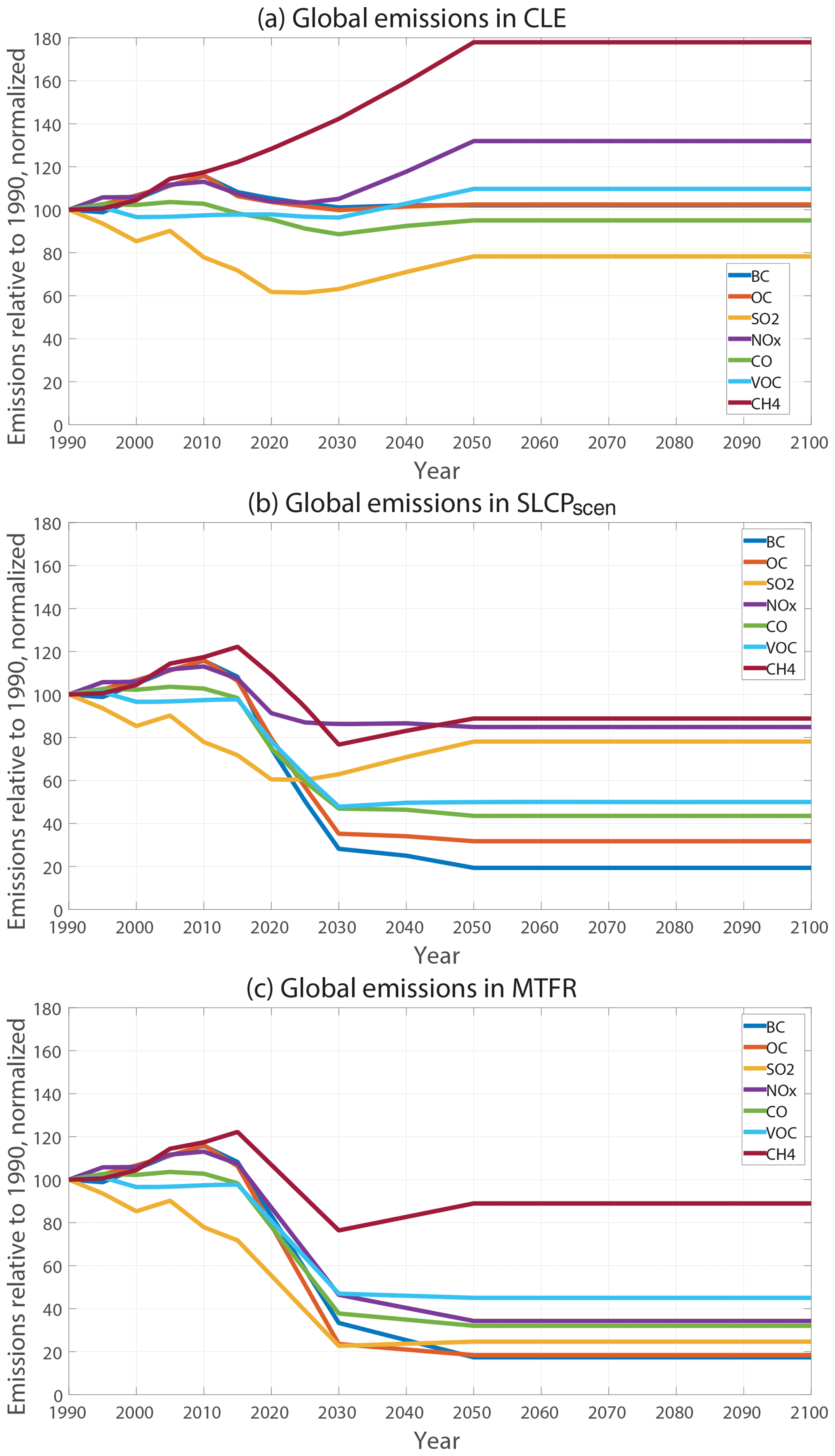
Figure 1The global emission levels relative to the 1990 level for baseline (a) CLE, (b) SLCPscen, and (c) MTFR. The 1990 emission level for each SLCF is normalized to 100.
2.2 SLCF mitigation pathways
As we are interested in how much mitigation of SLCFs can contribute towards reducing global and regional temperatures in the next decades, we construct two mitigation datasets from these pathways. The first is the emission difference between the mitigation scenario SLCPscen (see Fig. 1b) relative to the baseline CLE (see Fig. 1a). The second is the emission difference between the mitigation scenario MTFR (Fig. 1c) relative to the baseline. As the MTFR dataset in the ECLIPSE project is only given for the 2030–2050 period, we assume a linear trend between 2015 and 2030 for MTFR. We use the most recent version of the datasets, ECLIPSE V5a (IIASA, 2016). The ECLIPSE dataset is very detailed. Here, we aggregate regionally and seasonally as necessary to match the format of the ARTP values available (Aamaas et al., 2017). We interpolate linearly between the emissions points, which are given every five years and in some cases every 10 or 20 years. Since the emission scenarios from ECLIPSE go until 2050, we keep emission levels constant between 2050 and 2100 as we are not aware of any scenarios that are compatible with the ECLIPSE scenarios and contain the level of detail needed for our analysis. A large share of the emissions are also mitigated by 2050; hence, the temperature potential of further emission cuts after 2050 is limited.
2.3 Regional temperature potentials (ARTP)
The ARTP values applied come from the study by Aamaas et al. (2017). They give values for each species for emissions occurring in Europe (EUR), East Asia (EAS), global shipping (SHP), and the rest of the world (ROW), as well as separating between Northern Hemisphere summer and winter emissions. The temperature response is given for four latitude response bands (90–28∘ S, 28∘ S–28∘ N, 28–60∘ N, and 60–90∘ N). The temperature response in latitude band l in year t is given by a convolution:
for species i emitted in region r from emission sector s during season u (the year is divided into two seasons, with summer u=1 and winter u=2). The emission difference between a mitigation scenario and the reference scenario is ΔE. As the final year in the ECLIPSE emission scenarios is 2050, our main case is the temperature impact in 2050. The global temperature change is calculated as the area-weighted sum of the net regional changes given by Eq. (1).
The ARTP datasets utilized here are presented in detail by Aamaas et al. (2017), including how they were estimated, the processes included, and the robustness. That paper built on RF values calculated by Bellouin et al. (2016). The paper applied four different coupled chemistry–climate models or CTMs. They compared control simulations with perturbed simulations where emissions were reduced by 20 % for one species and one emission region. We apply the average values across models. For the aerosols and aerosol precursors, three out of four models included the aerosol direct and first indirect (cloud albedo) effect. RF for BC deposition on snow and ice surfaces and the semi-direct effect was estimated in one of the models. For the ozone precursors (NOx, CO, and VOC) and CH4, RF is modeled for the aerosol direct effect and first indirect effects, short-lived ozone effect, methane effect, and methane-induced ozone effect. Nitrate aerosols are also considered based on results from one model.
The matrix of regional response coefficients (RCS), which enables us to go from regional RFs to regional temperature responses and ARTPs, are also presented in detail by Aamaas et al. (2017). The RCS values are mostly based on coefficients modeled by Shindell and Faluvegi (2009). A weakness with our chosen method is that Shindell and Faluvegi (2009) is, to our knowledge, the only study that provides the necessary relationships between regional RFs and regional temperatures to create RCS values.
Uncertainties (1 SD – standard deviation) in the global temperature response have been estimated given a Monte Carlo analysis of 100 000 simulations. This analysis is based on a probability density function defined by model-based estimates of uncertainties in direct radiative forcing, from the literature (Myhre et al., 2013a, b), with the same treatment of radiative forcing uncertainty as in Lund et al. (2017) (see also the Supplement). Radiative forcing from each species is treated as a random variable. The distribution for the total uncertainty is derived by summing the probability density functions of all species. We assume that the radiative forcing uncertainties are independent in these calculations. Previous work by Aamaas et al. (2016) shows that the assumption of independent radiative forcing uncertainties gives a total uncertainty range for emission reductions for a mix of species that is similar to the range seen between different models. Further, they also found robustness for the method we use here to estimate temperature changes, such as models agreeing on whether different mitigation scenarios lead to warming or cooling. Also, note that the multi-model studies used as input were run with unified emissions. This particularly affects BC, where the current substantial uncertainty in annual emissions (Bond et al., 2013; Cohen and Wang, 2014) will not be represented. We compare our derived uncertainties to the influence of low and high climate sensitivities in the literature, 1.5 and 4.5 ∘C for a doubling of CO2 (Bindoff et al., 2013). Here, we adopt a lognormal distribution and assume the value range covers 1 SD. Uncertainties are not given for the latitude bands as a formal quantification of uncertainties for the ARTPs has not been produced.
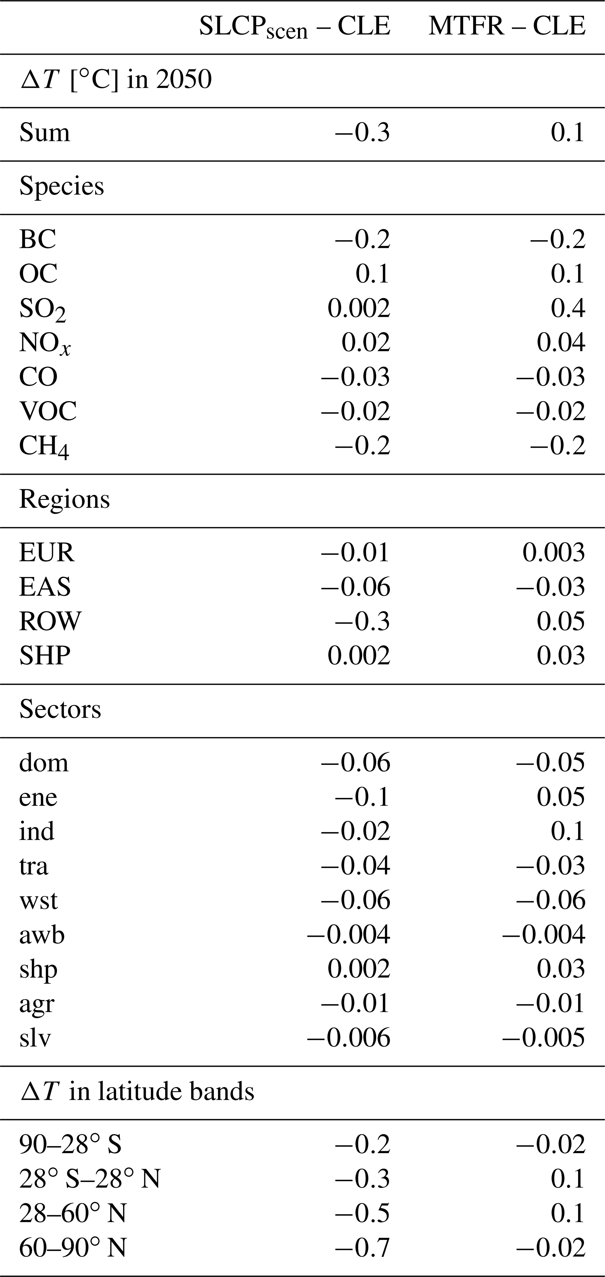
As our analysis can be viewed from multiple dimensions; we present the results by focusing on one dimension at a time. An overview of our temperature response estimates relative to the baseline is given in Table 2; the estimates are presented in detail in the following sections. Temperature effects in 2050 are presented for the global and regional level, for species, for emission regions, and for emission sectors.
Table 2The global and regional temperature responses in 2050 for SLCPscen and MTFR scenarios relative to the baseline CLE. Global temperature responses are given for the net, as well as for all the species, emission regions, and emission sectors at a global level. In the lower part, temperature responses in the four latitude bands are shown for global emissions. This table is a synthesis of Figs. 2–4. The sectors included are agriculture (agr), agriculture waste burning (awb), domestic (dom), energy (ene), industry (ind), solvent (slv), transportation (tra), waste (wst), and shipping (shp).
3.1 Global temperature change
Figure 2 shows the temporal temperature response from 2010 to 2100 with the two scenarios relative to the baseline for the different species and the net response. As for the following figures, results for SLCPscen relative to the baseline are found in Fig. 2a and MTFR relative to the baseline in Fig 2b. If SLCFs are mitigated in a climate-optimal manner, we estimate a maximum change in global temperature of ∘C by 2050, relative to current legislation, increasing to about −0.4 ∘C later in the century ending at ∘C in 2100. (see Fig. 2a, black line, and Table 2). The temperature response of aggressive mitigation of SLCFs (MTFR) leads gradually to a small change in temperature of 0.1±0.1 ∘C in 2050 relative to the baseline, which seems to be counterproductive in terms of goals limiting the global temperature increase (see Fig. 2b). As the uncertainty interval is large, since large emission cuts of warming and cooling components almost cancel each other out (about 0.7 ∘C cooling and warming in 2050; see Fig. S3 in the Supplement for cooling and warming separated for both MTFR and SLCPscen), we cannot rule out that this scenario may lead to cooling. In the climate-optimal scenario (SLCPscen), CH4 ( ∘C in 2050 and increasing in magnitude) and BC ( ∘C in 2050) are the main drivers of the temperature reductions (Fig. 2a). The measures will also reduce co-emissions of cooling species, causing a warming from those of more than 0.2 ∘C in 2050. The main warming contributions are emission reductions of OC and NOx, with small impacts from other SLCFs. The main difference to the maximum reduction scenario (MTFR) is the large warming contribution for MTFR (0.4±0.1 ∘C in 2050) from SO2 reductions as well as additional warming from NOx reductions (Fig. 2b).

Figure 2Global temperature response due to the (a) SLCPscen and (b) MTFR scenarios relative to the baseline CLE scenario. Future global temperature change will also be impacted by historic and baseline emissions which are not accounted for here. Error bars representing 1 SD (standard deviation) are given for the net response in 2030, 2050, and 2100. They are calculated based on literature values for Gaussian uncertainties in per-component RF, assuming no interspecies correlation, and estimated using a Monte Carlo analysis (100 000 pulls), where component forcing values are drawn from within the uncertainty distributions.

Figure 3The temperature response in the latitude bands and globally in 2050 for emission regions and emission sectors for (a) SLCPscen and (b) MTFR scenarios relative to the baseline CLE. The emission regions are Europe (EUR), East Asia (EAS), global shipping (SHP), and the rest of the world (ROW). The net response in the latitude bands due to emissions from each emission region is given by the symbols. The emission sectors are agriculture (agr), agriculture waste burning (awb), domestic (dom), energy (ene), industry (ind), solvent (slv), transportation (tra), waste (wst), and shipping (shp).
3.2 Regional temperature change
The temperature responses in the four latitudinal bands are given in Fig. 3 for different emission regions and emission sectors; all responses are relative to the baseline. The global responses are found to the right, while the responses in the latitude bands from south to north are given from left towards right. The symbols are the net response for each emission region. In this section, we discuss differences in the response between the latitude bands. The Arctic (60–90∘ N) is the region that is the most sensitive to the mitigation scenarios for all emission regions (see Fig. 3 and Table 2), followed by northern midlatitudes (28–60∘ N), as the climate sensitivities are largest for those regions, and most of the emissions occur in the Northern Hemisphere (Aamaas et al., 2017). In SLCPscen, the cooling in the Arctic (−0.7 ∘C in 2050) is more than twice the global average. This sensitivity in the Arctic is larger than for reductions of CO2, which would be roughly 50 % when applying the ARTP concept to CO2. This amplification in the Arctic is larger than the average for mitigation of European emissions and smaller for mitigation of East Asian emissions (see Fig. 3a). Measures on BC emissions during winter in the Northern Hemisphere contribute to this amplification. In terms of sectors, mitigation measures on SLCFs from agriculture waste burning, domestic, transportation, and industry have larger than average influence on the Arctic relative to the global average (Fig. 4). Some variability is also seen for the Arctic. While MTFR will lead to warming globally relative to baseline CLE, a cooling of the same magnitude is estimated for the Arctic (see Fig. 3b). The net cooling in the Arctic is driven by emissions from rest of the world, while mitigation in the shipping sector leads to warming for both, and the net effect of European mitigation is near zero.
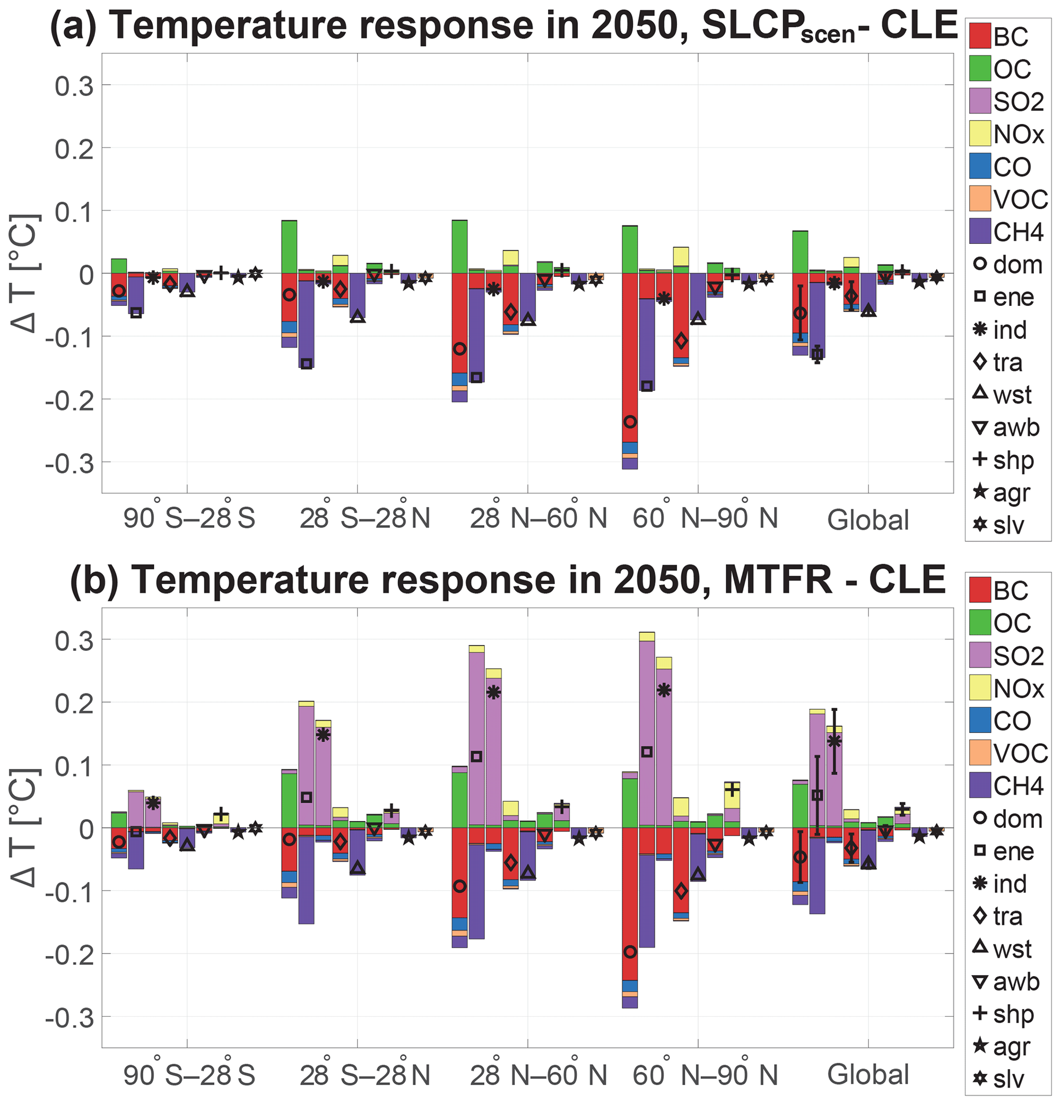
Figure 4The temperature response in the latitude bands and globally in 2050 for emission sectors and species for the (a) SLCPscen and (b) MTFR scenarios relative to the baseline CLE. Future global temperature change will also be impacted by historic and baseline emissions, which are not accounted for here. The emission sectors are agriculture (agr), agriculture waste burning (awb), domestic (dom), energy (ene), industry (ind), solvent (slv), transportation (tra), waste (wst), and shipping (shp). The net response in the latitude bands due to emissions from each emission sector is given by the symbols. Error bars representing 1 SD are given for the sectors for the global temperature response. They are calculated based on literature values for Gaussian uncertainties in per-component RF, assuming no interspecies correlation, and estimated using a Monte Carlo analysis (100 000 pulls), where component forcing values are drawn from within the uncertainty distributions.
3.3 Temperature change by emission region
The emission region that contributes the most in the mitigation scenarios is rest of the world (see Fig. 3 and Table 2). In the Supplement, we indicate that rest of Asia and other developing regions are the most important regions (as seen in Stohl et al., 2015), although our ARTP dataset limits us from making clear conclusions of what subregions have the largest cooling potential. In SLCPscen, mitigation leads to cooling from all emission regions and emission sectors except global shipping (Fig. 3a). In MTFR, warming globally is estimated for rest of the world and shipping, while near zero change for Europe and a cooling contribution for East Asia (Fig. 3b).
3.4 Temperature change by emission sector
In Fig. 4, the temperature responses in the four latitudinal bands are given for different emission sectors and separated by the emitted species; all responses are relative to the baseline. The emission sectors that give the largest cooling in SLCPscen are energy, domestic, waste, and transportation (see Fig. 4a and Table 2). In the Arctic, the order changes with domestic becoming the most important sector and transportation moved up to third place, mainly due to the large warming of BC in the Arctic. Shipping is the only sector that causes a small warming when mitigated. While MTFR led to a net warming, only three out of the nine sectors contribute to that, the industry, energy, and shipping sectors (Fig. 4b). Even for the energy sector, mitigation in East Asia leads to cooling (Fig. 3b). Most of the mitigation measures found unsuitable in a climate-optimal scenario can be placed in those sectors.
3.5 Uncertainties
In Fig. 5, the uncertainties for the global temperature responses in Figs. 3 and 4, based on uncertainties in radiative forcing, are compared to the uncertainty given different climate sensitivities. The uncertainties for the radiative forcing give generally a larger span than the climate sensitivity when a broad mix of emissions are mitigated, such as in the MTFR scenario. For individual components, the range in climate sensitivities leads to a larger span than uncertainty in radiative forcing.

Figure 5The global temperature response in 2050 in mitigation scenarios relative to the baseline for emission regions and emission sectors for SLCPscen and MTFR scenarios. Error bars representing 1 SD are included. The blue and black error bars are calculated based on literature values for Gaussian uncertainties in per-component RF, assuming no interspecies correlation, and estimated using a Monte Carlo analysis (100 000 pulls), where component forcing values are drawn from within the uncertainty distributions. The blue error bars indicate the uncertainty for the emission regions, the black error bars for the emission sectors. The grey error bars are estimated from uncertainty in the climate sensitivity, based on Monte Carlo analysis (100 000 pulls) with values drawn from within the lognormal uncertainty distribution.
The method applied here (Sect. 2.3) estimates the long-term response to a sustained change in SLCF emissions. However, in the current climate (now 2015), the climate has not reached the full response of sustained SLCF emissions at the current level due to the thermal inertia of the system. We have also estimated the temperature perturbations after 2015, running a transient simulation through 2015 using historic emissions of SLCFs and applying the same methodology as in Sect. 2.3. The potential for temperature reductions is reduced by up to 0.04 ∘C in 2050 and 0.05 ∘C in 2100 when this masked warming is included. Hence, the actual global temperature reduction is −0.3 ∘C by 2050 in SLCPscen when climate variability is excluded.
For the mean of the 2041–2050 period, our estimate of global temperature change of −0.29 ∘C, relative to the baseline, is higher than −0.22 ∘C calculated by Stohl et al. (2015), which may be due to the use of different versions of the ECLIPSE emission datasets, as well as some updates in the ARTP values.
A temperature change in 2050 of −0.3 ∘C in SLCPscen relative to the baseline could potentially offset a large increase in CO2 emissions. If we weight ARTP with a time horizon of 30 years, approximately the number of years until 2050, this temperature change is the same as about 520 Gt CO2, or 15 years of current global CO2 emissions. A climate optimal mitigation of SLCFs can therefore contribute to limiting the global temperature increase; however, this is only when considered in addition to sustained CO2 mitigation (e.g., Shoemaker et al., 2013).
SLCFs are mitigated due to different concerns, including that they contribute to achieving several of the Sustainable Development Goals (Shindell et al., 2017). Hence, while a climate-optimal mitigation strategy on SLCFs may be needed, in addition to reducing CO2 emissions, to contribute in avoiding global warming above the temperature targets in the Paris Agreement, measures undertaken to reduce air pollution and other problems are likely to lead to higher levels of warming. In this respect, climate-optimized mitigation of SLCFs can be considered as a type of geoengineering, as we keep emitting cooling substances. This is not an obvious or trivial choice due to the higher levels of air pollution it entails, and it would likely meet political resistance, as the ability to also address air pollution is seen as a main motivation for SLCF mitigation (Victor et al., 2015), although the two problems are viewed as interlinked (Tvinnereim et al., 2017). Thus, the feasibility of only executing the climate-optimal measures is lower than if there were no other concerns. SLCFs mitigation will lead to numerous other benefits, reducing health problems, increasing yields from agriculture, and achieving several of the sustainable development targets (UN, 2015; Haines et al., 2017). Many of the measures with the largest overall economic benefits involve SO2 reductions, measures that may be difficult for policymakers to neglect while prioritizing less beneficial measures that are climate-optimal. Another issue is the choice of baseline for evaluation of temperature change. We apply here the most recent ECLIPSE emission dataset from July 2015, while measures taken and planned legislation after that date will, in particular, lower SO2 emissions. The two main consequences are that the warming impact of MTFR is probably smaller or nonexistent and that limiting the global temperature increase to 1.5 ∘C is harder, as more SO2 emissions are removed than in a climate-optimal SLCF mitigation scenario.
SLCFs are also co-emitted with CO2. The ECLIPSE mitigation dataset makes use of external projections of energy use and industrial production and does not include mitigation measures directly on CO2. Stohl et al. (2015) argue that the measures included in this study have no significant impact on CO2 emissions. However, Rogelj et al. (2014) showed that mitigation of CO2 will lead to reductions of SLCFs. Hence, the potential cooling effect of dedicated reductions in emissions of warming SLCFs may be limited by successful mitigation of CO2. As global temperature may peak or stabilize some time after 2050, the temperature reduction by mitigating SLCFs can be seen as more critical at reducing this peak or level than reducing global temperature in 2050, the year we focus on in this study.
While the calculations here could also be based on AGTP values, Aamaas et al. (2017) argue that the regionality and seasonality included in the emission dataset and in the metric value give added value. Regional responses, such as the higher efficacy in the Arctic due to emissions close to the Arctic are better captured than global averages. Users of these results may also find estimated temperature responses in latitude bands more interesting than a global average. While previous studies have used ARTP values to calculate the temperature impact of SLCF mitigation globally (Stohl et al., 2015) and in the Arctic (Sand et al., 2016), we also show the temperature impact in the regions where most people live, such as in the 28–60∘ N latitude band. For this band, the net temperature reduction in 2050 in the SLCPscen scenario relative to the baseline is 0.5 ∘C, or almost 50 % larger than the global average.
Emission metrics are based on the current atmospheric composition and linearity; hence, an 80 % reduction of a pollutant is assumed to give twice the impact of a 40 % reduction. While this holds for small perturbations, this assumption may be inaccurate for the large SLCF reductions by 2050 in the SLCPscen and MTFR scenarios. Chen et al. (2018) recently quantified the uncertainties by assuming linearity and found an error of up to 15 % for the direct radiative forcing efficiency for BC and OC when assuming a total phaseout of emissions. The uncertainties can be larger for the indirect radiative forcing, especially in high emitting regions. Another assumption is the choice of constant emissions after 2050. This was chosen as we were unable to combine with other scenarios with emission data after 2050; a reduction of emissions to varying degree in all three scenarios may occur after 2050. Newer studies (e.g., Stjern et al., 2017; Baker et al., 2015) have also shown that the warming of BC emissions is smaller than implicitly included with the emission metric values used here; hence, the cooling potential of reducing BC emissions is likely smaller than estimated by us. However, our dataset is in the lower end of the range given by Samset et al. (2018) (0.5–1.1 ∘C for removing all anthropogenic emissions of BC, OC, and SO2) and thus not outside of the likely range given by state-of-the-art knowledge.
Different stakeholders may be interested in different aspects of our calculations. Decision makers can easily combine their own emission datasets with ARTP values to investigate what is most relevant for them. As the dimensions are many, we present additional figures in the Supplement, such as what the regional temperature change is for different times throughout the 21st century.
This study has not analyzed scenarios with CO2 mitigation or measures on SLCFs that will also result in emission cuts of CO2. However, we have estimated the temperature effects of different air quality measures on SLCFs emissions. We have shown that mitigation of SLCFs can contribute to reducing global and regional temperatures in the next few decades if mitigation is optimized with regards to temperature change. On the other hand, mitigation of SLCFs to gain other benefits can be counterproductive for limiting the temperature increase, especially if we cut emissions of SO2. A global temperature reduction from SLCF mitigation of about ∘C is technically feasible in the second part of the 21st century. Emission reductions of CH4 and BC will contribute the most. The sectors with the largest shares contributing to cooling are energy, domestic, waste, and transportation in the SLCPscen scenario, while aggressive emission cuts will lead to warming from industry, energy, and shipping. The net response in the SLCPscen scenario is almost 50 % larger than the global average for the 28–60∘ N latitude band and more than double the response in the Arctic. BC emissions drive this, as BC emissions during winter in the Northern Hemisphere will have much larger contribution than when looking at global and annual averages. The Arctic is the most influenced by mitigation in the domestic, energy, and transportation sectors. The feasible temperature reductions may be smaller than those estimated here due to several reasons, such as the entangling of SLCFs and CO2 emissions, the unlikely option by policymakers of leaving out measures that are highly beneficial for health that are not climate-optimal, and newer studies indicating a smaller temperature impact of BC emissions.
The analysis is based on two datasets. The ECLIPSE emission data can be downloaded from http://www.iiasa.ac.at/web/home/research/researchPrograms/air/ECLIPSEv5a.html (IIASA, 2016). The ARTP values applied can be found in Aamaas et al. (2017).
The supplement related to this article is available online at: https://doi.org/10.5194/acp-19-15235-2019-supplement.
TKB and BA developed the idea of the study. BA compiled the needed data and modeled the regional temperature responses. BA led the writing of the paper, with contributions from TKB and BHS.
The authors declare that they have no conflict of interest.
We thank Zbigniew Klimont for help with the ECLIPSE emission dataset and Steffen Kallbekken for commenting a draft version of this article.
This research has been supported by the The Research Council of Norway (grant no. 261728).
This paper was edited by Pedro Jimenez-Guerrero and reviewed by two anonymous referees.
Aamaas, B., Berntsen, T. K., Fuglestvedt, J. S., Shine, K. P., and Bellouin, N.: Regional emission metrics for short-lived climate forcers from multiple models, Atmos. Chem. Phys., 16, 7451–7468, https://doi.org/10.5194/acp-16-7451-2016, 2016.
Aamaas, B., Berntsen, T. K., Fuglestvedt, J. S., Shine, K. P., and Collins, W. J.: Regional temperature change potentials for short lived climate forcers based on radiative forcing from multiple models, Atmos. Chem. Phys., 17, 10795–10809, https://doi.org/10.5194/acp-17-10795-2017, 2017.
Amann, M., Klimont, Z., and Wagner, F.: Regional and Global Emissions of Air Pollutants: Recent Trends and Future Scenarios, Annu. Rev. Environ. Resour., 38, 31–55, https://doi.org/10.1146/annurev-environ-052912-173303, 2013.
Baker, L. H., Collins, W. J., Olivié, D. J. L., Cherian, R., Hodnebrog, O., Myhre, G., and Quaas, J.: Climate responses to anthropogenic emissions of short-lived climate pollutants, Atmos. Chem. Phys., 15, 8201–8216, https://doi.org/10.5194/acp-15-8201-2015, 2015.
Bellouin, N., Baker, L., Hodnebrog, Ø., Olivié, D., Cherian, R., Macintosh, C., Samset, B., Esteve, A., Aamaas, B., Quaas, J., and Myhre, G.: Regional and seasonal radiative forcing by perturbations to aerosol and ozone precursor emissions, Atmos. Chem. Phys., 16, 13885–13910, https://doi.org/10.5194/acp-16-13885-2016, 2016.
Berntsen, T., Tanaka, K., and Fuglestvedt, J.: Does black carbon abatement hamper CO2 abatement?, Climatic Change, 103, 627–633, https://doi.org/10.1007/s10584-010-9941-3, 2010.
Bindoff, N. L., Stott, P. A., AchutaRao, K. M., Allen, M. R., Gillett, N., Gutzler, D., Hansingo, K., Hegerl, G., Hu, Y., Jain, S., Mokhov, I. I., Overland, J., Perlwitz, J., Sebbari, R., and Zhang, X.: Detection and Attribution of Climate Change: from Global to Regional, in: Climate Change 2013: The Physical Science Basis, Contribution of Working Group I to the Fifth Assessment Report of the Intergovernmental Panel on Climate Change, edited by: Stocker, T. F., Qin, D., Plattner, G.-K., Tignor, M., Allen, S. K., Boschung, J., Nauels, A., Xia, Y., Bex, V., and Midgley, P. M., Cambridge University Press, Cambridge, UK and New York, NY, USA, 867–952, 2013.
Bond, T. C., Doherty, S. J., Fahey, D. W., Forster, P. M., Berntsen, T., DeAngelo, B. J., Flanner, M. G., Ghan, S., Kärcher, B., Koch, D., Kinne, S., Kondo, Y., Quinn, P. K., Sarofim, M. C., Schultz, M. G., Schulz, M., Venkataraman, C., Zhang, H., Zhang, S., Bellouin, N., Guttikunda, S. K., Hopke, P. K., Jacobson, M. Z., Kaiser, J. W., Klimont, Z., Lohmann, U., Schwarz, J. P., Shindell, D., Storelvmo, T., Warren, S. G., and Zender, C. S.: Bounding the role of black carbon in the climate system: A scientific assessment, J. Geophys. Res.-Atmos., 118, 5380–5552, https://doi.org/10.1002/jgrd.50171, 2013.
Chen, Y., Wang, H., Singh, B., Ma, P.-L., Rasch, P. J., and Bond, T. C.: Investigating the linear dependence of direct and indirect radiative forcing on emission of carbonaceous aerosols in a global climate model, J. Geophys. Res.-Atmos., 123, 1657–1672, https://doi.org/10.1002/2017JD027244, 2018.
Cohen, J. B. and Wang, C.: Estimating global black carbon emissions using a top-down Kalman Filter approach, J. Geophys. Res.-Atmos., 119, 307–323, https://doi.org/10.1002/2013jd019912, 2014.
Di, Q., Wang, Y., Zanobetti, A., Wang, Y., Koutrakis, P., Choirat, C., Dominici, F., and Schwartz, J. D.: Air Pollution and Mortality in the Medicare Population, New Engl. J. Med., 376, 2513–2522, https://doi.org/10.1056/NEJMoa1702747, 2017.
Dockery, D. W., Pope, C. A., Xu, X., Spengler, J. D., Ware, J. H., Fay, M. E., Ferris, B. G., and Speizer, F. E.: An Association between Air Pollution and Mortality in Six U.S. Cities, New Engl. J. Med., 329, 1753–1759, https://doi.org/10.1056/nejm199312093292401, 1993.
IIASA: ECLIPSE V5a global emission fields, available at: http://eclipse.nilu.no/ (last access: 21 April 2017), 2016.
Haines, A., Amann, M., Borgford-Parnell, N., Leonard, S., Kuylenstierna, J., and Shindell, D.: Short-lived climate pollutant mitigation and the Sustainable Development Goals, Nat. Clim. Change, 7, 863–869, https://doi.org/10.1038/s41558-017-0012-x, 2017.
Klimont, Z., Kupiainen, K., Heyes, C., Purohit, P., Cofala, J., Rafaj, P., Borken-Kleefeld, J., and Schoepp, W.: Global anthropogenic emissions of particulate matter including black carbon, Atmos. Chem. Phys., 17, 8681–8723, https://doi.org/10.5194/acp-17-8681-2017, 2017.
Klimont, Z., Höglund-Isaksson, L., Heyes, C., Rafaj, P., Schöpp, W., Cofala, J., Purohit, P., Borken-Kleefeld, J., Kupiainen, K., Kiesewetter, G., Winiwarter, W., Amann, M., Zhao, B., Wang, S. X., Bertok, I., and Sander, R.: Global scenarios of air pollutants and methane: 1990–2050, in preparation, 2019.
Li, C., McLinden, C., Fioletov, V., Krotkov, N., Carn, S., Joiner, J., Streets, D., He, H., Ren, X., Li, Z., and Dickerson, R. R.: India Is Overtaking China as the World's Largest Emitter of Anthropogenic Sulfur Dioxide, Scient. Rep., 7, 14304, https://doi.org/10.1038/s41598-017-14639-8, 2017.
Lund, M. T., Aamaas, B., Berntsen, T., Bock, L., Burkhardt, U., Fuglestvedt, J. S., and Shine, K. P.: Emission metrics for quantifying regional climate impacts of aviation, Earth Syst. Dynam., 8, 547–563, https://doi.org/10.5194/esd-8-547-2017, 2017.
Myhre, G., Samset, B. H., Schulz, M., Balkanski, Y., Bauer, S., Berntsen, T. K., Bian, H., Bellouin, N., Chin, M., Diehl, T., Easter, R. C., Feichter, J., Ghan, S. J., Hauglustaine, D., Iversen, T., Kinne, S., Kirkevåg, A., Lamarque, J. F., Lin, G., Liu, X., Lund, M. T., Luo, G., Ma, X., van Noije, T., Penner, J. E., Rasch, P. J., Ruiz, A., Seland, Ø., Skeie, R. B., Stier, P., Takemura, T., Tsigaridis, K., Wang, P., Wang, Z., Xu, L., Yu, H., Yu, F., Yoon, J. H., Zhang, K., Zhang, H., and Zhou, C.: Radiative forcing of the direct aerosol effect from AeroCom Phase II simulations, Atmos. Chem. Phys., 13, 1853–1877, https://doi.org/10.5194/acp-13-1853-2013, 2013a.
Myhre, G., Shindell, D., Bréon, F.-M., Collins, B., Fuglestvedt, J. S., Huang, J., Koch, D., Lamarque, J.-F., Lee, D., Mendoza, B., Nakajima, T., Robock, A., Stephens, G., Takemura, T., and Zhang, H.: Anthropogenic and Natural Radiative Forcing, in: Climate Change 2013: The Physical Science Basis, Contribution of Working Group I to the Fifth Assessment Report of the Intergovernmental Panel on Climate Change, edited by: Stocker, T. F., Qin, D., Plattner, G. K., Tignor, M., Allen, S. K., Boschung, J., Nauels, A., Xia, Y., Bex, V., and Midgley, P. M., Cambridge University Press, Cambridge, UK and New York, NY, USA, 2013b.
Myhre, G., Aas, W., Cherian, R., Collins, W., Faluvegi, G., Flanner, M., Forster, P., Hodnebrog, Ø., Klimont, Z., Lund, M. T., Mülmenstädt, J., Lund Myhre, C., Olivié, D., Prather, M., Quaas, J., Samset, B. H., Schnell, J. L., Schulz, M., Shindell, D., Skeie, R. B., Takemura, T., and Tsyro, S.: Multi-model simulations of aerosol and ozone radiative forcing due to anthropogenic emission changes during the period 1990–2015, Atmos. Chem. Phys., 17, 2709–2720, https://doi.org/10.5194/acp-17-2709-2017, 2017.
Pierrehumbert, R.: Short-Lived Climate Pollution, Annu. Rev. Earth Planet. Sci., 42, 341–379, https://doi.org/10.1146/annurev-earth-060313-054843, 2014.
Rafaj, P., Amann, M., Siri, J., and Wuester, H.: Changes in European greenhouse gas and air pollutant emissions 1960–2010: decomposition of determining factors, in: Uncertainties in Greenhouse Gas Inventories: Expanding Our Perspective, edited by: Ometto, J. P., Bun, R., Jonas, M., and Nahorski, Z., Springer International Publishing, Cham, 27–54, 2015.
Rao, S., Klimont, Z., Smith, S. J., Van Dingenen, R., Dentener, F., Bouwman, L., Riahi, K., Amann, M., Bodirsky, B. L., van Vuuren, D. P., Aleluia Reis, L., Calvin, K., Drouet, L., Fricko, O., Fujimori, S., Gernaat, D., Havlik, P., Harmsen, M., Hasegawa, T., Heyes, C., Hilaire, J., Luderer, G., Masui, T., Stehfest, E., Strefler, J., van der Sluis, S., and Tavoni, M.: Future air pollution in the Shared Socio-economic Pathways, Global Environ. Change, 42, 346–358, https://doi.org/10.1016/j.gloenvcha.2016.05.012, 2017.
Rogelj, J., Schaeffer, M., Meinshausen, M., Shindell, D. T., Hare, W., Klimont, Z., Velders, G. J. M., Amann, M., and Schellnhuber, H. J.: Disentangling the effects of CO2 and short-lived climate forcer mitigation, P. Natl. Acad. Scu. USA, 111, 16325–16330, https://doi.org/10.1073/pnas.1415631111, 2014.
Samset, B. H., Sand, M., Smith, C. J., Bauer, S. E., Forster, P. M., Fuglestvedt, J. S., Osprey, S., and Schleussner, C. F.: Climate impacts from a removal of anthropogenic aerosol emissions, Geophys. Res. Lett., 45, 1020–1029, https://doi.org/10.1002/2017GL076079, 2018.
Sand, M., Berntsen, T. K., von Salzen, K., Flanner, M. G., Langner, J., and Victor, D. G.: Response of Arctic temperature to changes in emissions of short-lived climate forcers, Nat. Clim. Change, 6, 286–289, https://doi.org/10.1038/nclimate2880, 2016.
Shindell, D. and Faluvegi, G.: Climate response to regional radiative forcing during the twentieth century, Nat. Geosci., 2, 294–300, 2009.
Shindell, D. and Faluvegi, G.: The net climate impact of coal-fired power plant emissions, Atmos. Chem. Phys., 10, 3247–3260, https://doi.org/10.5194/acp-10-3247-2010, 2010.
Shindell, D., Borgford-Parnell, N., Brauer, M., Haines, A., Kuylenstierna, J. C. I., Leonard, S. A., Ramanathan, V., Ravishankara, A., Amann, M., and Srivastava, L.: A climate policy pathway for near- and long-term benefits, Science, 356, 493–494, https://doi.org/10.1126/science.aak9521, 2017.
Shine, K. P., Fuglestvedt, J. S., Hailemariam, K., and Stuber, N.: Alternatives to the Global Warming Potential for Comparing Climate Impacts of Emissions of Greenhouse Gases, Climatic Change, 68, 281–302, https://doi.org/10.1007/s10584-005-1146-9, 2005.
Shine, K. P., Berntsen, T., Fuglestvedt, J. S., Stuber, N., and Skeie, R. B.: Comparing the climate effect of emissions of short and long lived climate agents, Philos. T. Roy. Soc. A, 365, 1903–1914, 2007.
Shoemaker, J. K., Schrag, D. P., Molina, M. J., and Ramanathan, V.: What Role for Short-Lived Climate Pollutants in Mitigation Policy?, Science, 342, 1323–1324, https://doi.org/10.1126/science.1240162, 2013.
Stjern, C. W., Samset, B. H., Myhre, G., Forster, P. M., Hodnebrog, Ø., Andrews, T., Boucher, O., Faluvegi, G., Iversen, T., Kasoar, M., Kharin, V., Kirkevåg, A., Lamarque, J.-F., Olivié, D., Richardson, T., Shawki, D., Shindell, D., Smith, C. J., Takemura, T., and Voulgarakis, A.: Rapid Adjustments Cause Weak Surface Temperature Response to Increased Black Carbon Concentrations, J. Geophys. Res.-Atmos., 122, 11462–11481, https://doi.org/10.1002/2017JD027326, 2017.
Stohl, A., Aamaas, B., Amann, M., Baker, L. H., Bellouin, N., Berntsen, T. K., Boucher, O., Cherian, R., Collins, W., Daskalakis, N., Dusinska, M., Eckhardt, S., Fuglestvedt, J. S., Harju, M., Heyes, C., Hodnebrog, O., Hao, J., Im, U., Kanakidou, M., Klimont, Z., Kupiainen, K., Law, K. S., Lund, M. T., Maas, R., MacIntosh, C. R., Myhre, G., Myriokefalitakis, S., Olivie, D., Quaas, J., Quennehen, B., Raut, J.-C., Rumbold, S. T., Samset, B. H., Schulz, M., Seland, O., Shine, K. P., Skeie, R. B., Wang, S., Yttri, K. E., and Zhu, T.: Evaluating the climate and air quality impacts of short-lived pollutants, Atmos. Chem. Phys., 15, 10529–10566, https://doi.org/10.5194/acp-15-10529-2015, 2015.
Tvinnereim, E., Liu, X., and Jamelske, E. M.: Public perceptions of air pollution and climate change: different manifestations, similar causes, and concerns, Climatic Change, 140, 399–412, https://doi.org/10.1007/s10584-016-1871-2, 2017.
UN: Transforming our world: the 2030 agenda for sustainable development, United Nations, New York, 2015.
UNEP: The Emissions Gap Report 2016, United Nations Environment Programme, Nairobi, 2016.
Victor, D. G., Zaelke, D., and Ramanathan, V.: Soot and short-lived pollutants provide political opportunity, Nat. Clim. Change, 5, 796–798, https://doi.org/10.1038/nclimate2703, 2015.
von Schneidemesser, E., Monks, P. S., Allan, J. D., Bruhwiler, L., Forster, P., Fowler, D., Lauer, A., Morgan, W. T., Paasonen, P., Righi, M., Sindelarova, K., and Sutton, M. A.: Chemistry and the Linkages between Air Quality and Climate Change, Chem. Rev., 115, 3856–3897, https://doi.org/10.1021/acs.chemrev.5b00089, 2015.
WHO: Ambient air pollution: A global assessment of exposure and burden of disease, World Health Organization, Geneva, 2016.