Impact of humidity biases on light precipitation occurrence: observations versus simulations

This work uses a network of GPS stations over Europe from which a homogenized integrated water vapor (IWV) dataset has been retrieved, completed with colocated temperature and precipitation measurements over specific stations to (i) estimate the biases of six regional climate models over Europe in terms of humidity; (ii) understand their origins; and (iii) finally assess the impact of these biases on the frequency of occurrence of precipitation. The evaluated simulations have been performed in the framework of HYMEX/Med-CORDEX programs and cover the Mediterranean area and part of Europe at horizontal resolutions of 50 to 12 km.

The analysis shows that models tend to overestimate the low values of IWV and the use of the nudging technique reduces the differences between GPS and simulated IWV. Results suggest that physics of models mostly explain the mean biases, while dynamics affects the variability. The land surface–atmosphere exchanges affect the estimation of IWV over most part of Europe, especially in summer. The limitations of the models to represent these processes explain part of their biases in IWV. However, models correctly simulate the dependance between IWV and temperature, and specifically the deviation that this relationship experiences regarding the Clausius–Clapeyron law after a critical value of temperature (T_break). The high spatial variability of T_break indicates that it has a strong dependence on local processes which drive the local humidity sources. This explains why the maximum values of IWV are not necessarily observed over warmer areas, which are often dry areas.

Finally, it is shown over the SIRTA observatory (near Paris) that the frequency of occurrence of light precipitation is strongly conditioned by the biases in IWV and by the precision of the models to reproduce the distribution of IWV as a function of the temperature. The results of the models indicate that a similar dependence occurs in other areas of Europe, especially where precipitation has a predominantly convective character. According to the observations, for each range of temperature, there is a critical value of IWV from which precipitation starts to increase. The critical values and the probability of exceeding them are simulated with a bias that depends on the model. Those models, which generally present light precipitation too often, show lower critical values and higher probability of exceeding them.

1 Introduction

Humidity plays a major role in the water and energy cycles due to its strong radiative effect associated with a positive feedback on climate (Randall et al., 2007) and its importance to control precipitation and particularly extreme ones (Held and Soden, 2006; Neelin et al., 2009; Sahany et al., 2012). Trends and variability of humidity and precipitation are strongly correlated (Trenberth et al., 2003; Zhang et al., 2013) and several studies have revealed that the rate of increase in daily extreme precipitation is highly connected with the warming following the Clausius–Clapeyron (C-C) relation (Allen and Ingram, 2002; Pall et al., 2007; Kharin et al., 2007). This rate of precipitation is indeed affected by the humidity content of the atmosphere (integrated water vapor, IWV), which rises as the climate warms (e.g., Trenberth, 2011). Nevertheless, dynamical processes (O'Gorman and Schneider, 2009; Sugiyama et al., 2010; Singleton and Toumi, 2013; Muller, 2013; Drobinski et al., 2016), lack of humidity sources leading to a decrease in relative humidity (RH; Drobinski et al., 2018), or low or high precipitation efficiency (Drobinski et al., 2016; Trenberth et al., 2003) can explain the deviation from C-C rate locally. Humidity variability at regional scale – and not only at the surface – thus needs to be assessed to better anticipate the precipitation change, and more specifically the rate of heavy precipitation, which are not well estimated by global models (e.g., Allan and Soden, 2008).

Another aspect that links IWV and precipitation concerns the triggering of precipitation and thus the frequency of occurrence of precipitation: Holloway and Neelin (2009) showed that precipitation over the tropical oceans is strongly sensitive to free-tropospheric humidity even more than surface humidity, and Neelin et al. (2009) and Sahany et al. (2012) further conclude that there exists a threshold of IWV, which depends on the mean tropospheric temperature, over which precipitation starts to increase significantly. They also showed that this critical value of IWV does not correspond to the saturation value when temperature increases, i.e., that at higher temperature, deep convection occurs at a lower value of relative humidity. This means that IWV is a relevant parameter to measure over long-term periods, at high temporal resolution and at the regional scale in order to establish the relationship between IWV–precipitation and temperature and monitor its possible evolution. Models still have strong difficulties in adequately simulating the water cycle (Trenberth et al., 2003; Flato et al., 2013), and often presents the “too often too light precipitation” problem (e.g., Sun et al., 2006; Panthou et al., 2016). A better knowledge of the IWV–precipitation relationship would be a help to better constrain models.

Up to now, very few long-term (> 15 years) and homogeneous datasets of water vapor measurements exist, even less at subdaily timescales. These datasets are necessary to understand the humidity variability at regional scales at different timescales. Besides, the colocation of such measurements with independent measurements of precipitation and vertical profiles of temperature provide a strong added value for better climate understanding. Reanalyses are of course a good tool to have these three parameters colocated over long-term and at subdaily timescales; however, precipitation mostly relies on the model physics. Moreover, Flato et al. (2013) have shown that even in reanalyses, the relationship between the IWV trend and the temperature trend presents differences between reanalyses and deviates from C-C over tropical oceans.

In this study, we make use of the Global Positioning System (GPS) IWV dataset that has been processed as done by Parracho et al. (2018) and which provides IWV measurements from over 100 European sites covering a period of 5 years or more. The GPS technique accurately measures IWV (accuracy around 1–2 kg m⁻² according to Bock et al., 2005, 2013, and Ning et al., 2016) in all weather conditions including rainy situations, which is an important aspect for our study (e.g., Wang et al., 2007). GPS measurements have been successfully used to better understand atmospheric processes at high resolution (Bastin et al., 2005, 2007; Bock et al., 2008; Champollion et al., 2009). Here we use a GPS IWV dataset to analyze the humidity biases in regional climate models over Europe at interannual, seasonal and daily timescales and to better understand the source of errors in models. We also use GPS IWV measurements colocated with precipitation and tropospheric temperature measurements from the SIRTA observatory in France to consider the relationships between these parameters. Note they have not yet been considered outside the tropics. We compare observations and regional models output at the site level and extend the analysis of models to other locations over Europe.

The paper is organized as follows: Sect. 2 presents the observational datasets and the different simulations used in this study. Section 3 describes the methodology to compare observations and models. In Sect. 4, the ability of models to reproduce the mean value of humidity and its variability over Europe at different timescales is evaluated. The influence of dynamical and physical processes is discussed, and a special focus on the scaling of IWV with temperature is developed. In Sect. 5, the issue of how much a bias in IWV can enhance the problem of “too often too light precipitation” behavior of models is raised by considering the relationship between mean tropospheric temperature, IWV and precipitation in the different models and observations over the SIRTA supersite in France. Then, by considering other stations across Europe, the generalization of this relationship is assessed. Finally, a conclusion is given in Sect. 6.

2 Material

2.1 GPS IWV data

The GPS dataset used in this study is based on homogeneously reprocessed GPS delay data produced by the NASA's Jet Propulsion Laboratory in the framework of the first International GNSS Service (IGS) reprocessing campaign. The data cover the period from January 1995 to May 2011 and include more than 400 stations globally. For the present study, the delay data were screened and converted into 6-hourly IWV estimates as described in Parracho et al. (2018). Then, daily values are computed using this 6-hourly dataset. The dataset was restricted to the period from January 1995 to December 2008 and includes 95 GPS stations over Europe as shown in Fig. 1. It represents many more stations than in the study of Parracho et al. (2018) because for the purpose of their study which estimates IWV trends, they restricted their selection to stations with only small gaps over the 15-year period from 1995 to 2010. Here, only stations with less than 5 years of observations are not considered in the evaluation of model humidity bias.

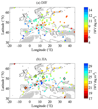
Figure 1 Mean values of IWV in winter (a) and summer (b) retrieved from GPS network. Note that color scales are different between winter and summer. Circles indicate stations with more than 10 years of observations between 1995 and 2008 and squares indicate stations with 5 to 10 years of observations. SIRTA observatory is shown by the black triangle. Black diamonds indicate the location of stations considered in Sect. 5.2. Topography higher than 500 m above sea level is shaded in grey.

2.2 Observations at SIRTA

This study also uses observations collected at the SIRTA atmospheric observatory, located 20 km southwest of Paris (48.7^∘ N, 2.2^∘ E at 160 m of altitude; black triangle in Fig. 1), from 2003 (Haeffelin et al., 2005). This observatory has collected many observations, which are now synthesized into the so-called “SIRTA-ReOBS dataset” described in Chiriaco et al. (2018a) and used in Chiriaco et al. (2014) and Bastin et al. (2018). After many steps of data quality control and harmonization, the “SIRTA-ReOBS” file contains hourly averages of more than 50 variables at this site. The sample of data varies from one variable to another. Among these variables, the IWV retrieved from GPS measurement since 2008 and the precipitation rate from a single rain gauge from 2003 to the present are available. A regional-scale precipitation estimate, deduced from the measurements of other Météo-France rain gauges located around Paris area, is also provided.

The Météo-France COMEPHORE (“COmbinaison en vue de la Meilleure Estimation de la Precipitation HOraiRE”) product is used to allow a fairer intercomparison between models and observations than the single rain gauge (Chen and Knutson, 2008): it is an hourly reanalysis of precipitation by merging radar data and rain gauges over France at 1 km×1 km resolution (more details in Fumière et al., 2019; see also Laurantin et al., 2012). From this product, we can have a better knowledge of the average precipitation rate over a model grid of 50 km×50 km or higher resolution. However, this product only covers the period 1997–2007 (at the time of this study) and is not concomitant with the IWV dataset over SIRTA. Despite this, a comparison has been made between the statistics of the different datasets when possible (see Sect. 3.2).

The Météo-France radiosoundings, launched twice a day from Trappes (near 00:00 and 12:00 UTC), 15 km to the west of SIRTA, are also used to compute the mean tropospheric temperature (more details in Sect. 3).

Table 1 List of models used in the study.

2.3 Med-CORDEX simulations

The list of regional climate models (RCMs) and details about the settings are given in Table 1. All the simulations use the 6-hourly European Center for Medium-Range Weather Forecast (ECMWF) reanalyses ERA-Interim (Dee et al., 2011) as RCM boundary conditions. They cover at least the period 1989–2008 as initially recommended in the MED-CORDEX project (Ruti et al., 2015). For LMDZ, which is a global model with regional zoom capability, temperature, wind speed and specific humidity are nudged towards the ERA-Interim fields outside the MED-CORDEX domain. It must be noted that the mesh of LMDZ is not regular within the zoom region and the resolution varies between 50 and 30 km. All other RCMs are forced at the boundaries using 3-dimensional re-analyses of wind, humidity, temperature or potential temperature, and geopotential height. For CCLM, cloud ice and liquid water are additionally prescribed at the domain boundaries. The IPSL WRF simulation uses nudging at all scales within the domain for temperature, wind and humidity above the planetary boundary layer (Salameh et al., 2010; Omrani et al., 2013, 2015). The other models did not use nudging in the Med-CORDEX domain.

Simulations used here were produced from five models (ALADIN V5.2, Colin et al., 2010; CCLM, Rockel et al., 2008; WRF V3.1.1, Skamarock et al., 2008; LMDZ V4, Hourdin et al., 2006; PROMES, Dominguez et al., 2010, 2013) with a horizontal resolution around 50 km (0.44^∘ for most models) on the MED-CORDEX domain. In the following the simulations are referred to by the name of the modeling group and resolution (see Table 1, first column). All the models provide daily values of IWV, precipitation, 2 m temperature and temperature at 850, 500 and 200 hPa.

2.4 Others datasets

The GPS observations are supplemented by the HadISD v.2.0.1.2016 subdaily dataset of surface parameters (e.g., temperature, dew point temperature, wind, pressure; Dunn et al., 2012). It is global and based on the Integrated Surface Database (ISD) dataset from NOAA's National Climatic Data Center. Stations were selected on the basis of their length of record and reporting frequency before they are passed through a suite of quality control tests. It is a joint effort from the MetOffice Hadley Center and the National Center for Atmospheric research (NCAR).

3 Methods

To compare models and observations, we consider differences as the “model minus observation” results throughout the paper.

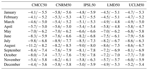
Table 2 Values of linear regression slopes obtained for each model/each month when plotting IWVmod–IWVobs as a function of the difference in altitudes between model and GPS at each station. The first figure is for native grid of the model and the second figure is for model regridded to ERAI grid. It is expressed in 10⁻³ kg m⁻³.

3.1 Comparison between GPS dataset and model outputs

Each modeling group has provided a file containing the gridded IWV over the 1995–2008 period at daily resolution on its native grid. The IWV is either computed online or offline in the model. The offline computation can introduce some errors due to vertical integration over the discretized vertical grid. For each model, we extracted the value of IWV at the closest grid point of GPS stations. We did it using the native grid, and also after having regridded all the model outputs to ERA-Interim (ERAI) grid, to have a fair comparison with ERAI when necessary. The difference in altitude between the GPS station and the closest grid point is difficult to take into account and can introduce strong bias over complex terrain (Hagemann et al., 2003; Wang and Zhang, 2009). As a consequence, the stations where the difference in altitude is higher than 500 m were removed from the analysis. Note the number of stations that are removed depends on each model since the models do not use the same topography and the same projection. Then, a linear correction is applied on model outputs to reduce the bias due to orography: for each model and each month, we plotted the difference in the monthly averaged IWV values between the model and GPS as a function of the difference in altitude and we concluded that a linear correction can be applied to take into account the difference in altitude. For each different month, the slope of the linear regression between these two differences is computed and we apply the corresponding correction to IWV values of the model. The values of the slope of the linear regression for each model and each month are indicated in Table 2, both for the native grid of the model and for the regridded outputs. Various evaluation metrics (Table 3) have been computed with and without correction for these two grids. The correction does not impact the variability scores (e.g., interannual variability), but does affect the mean bias (not always by an improvement) and slightly reduces the standard deviation of the difference (Table 3). It does not affect the ranking of performance between models.

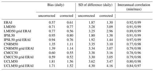
Table 3 Mean bias and standard deviation (SD) in kilograms per meter (kg m⁻²) of the differences in IWV between models and GPS observations using daily time resolution, and using the data obtained with the correction due to altitude difference or without it. Computation has been done using models on their native grid, or bilinearly remapped on the ERA-Interim grid. The rightmost column indicates the minimum and maximum values of the correlation of the interannual variability of monthly GPS anomalies and model anomalies (one correlation computed by month).

Note that at SIRTA, the difference in altitude is weak and results are thus not impacted by this problem.

3.2 Comparison with SIRTA observations

The following comparisons were made with SIRTA observations:

• Tropospheric temperature. To be as consistent as possible between model outputs and radiosoundings, the mean tropospheric temperature corresponds here to the daily average value of 2 m temperature, and temperatures at 850, 500 and 200 hPa. So we extracted the temperature values at these pressure levels for each radiosounding launched from Trappes (a few kilometers away from SIRTA) and computed the mean tropospheric temperature as the average of these four values. Then, the daily mean is the average of the two daily radiosoundings. The same method is applied to ERA-Interim reanalysis to compute the mean tropospheric temperature over the other European sites. The impact of using ERA-Interim instead of radiosounding data has been evaluated at SIRTA where both are available. Due to the width of temperature bins considered in this study, results are not sensitive to the use of one or another.

• Precipitation. The first step consists of comparing the precipitation statistics obtained using the single rain gauge located at SIRTA, from the closest grid point (1 km×1 km) of COMEPHORE over the SIRTA and an average of COMEPHORE over an area centered over the SIRTA and covering 2500 km² (i.e., a 50 km resolution model grid point). Figure 2 shows the mean annual cycle of the frequency of occurrence of different light precipitation regimes. The annual cycle is computed from 30-day means from January to December over the years 2004–2007, which is the common period of all datasets. The SIRTA rain gauge and COMEPHORE product do not indicate the same frequency of occurrence of nonprecipitating days, and very light precipitation, but they show similar frequency of occurrence for light precipitation which corresponds mainly to large-scale precipitation. Note the different values of the 50th percentile of precipitation when considering only precipitating days, which emphasize the impact of heavy precipitation on the estimate of this index. The SIRTA rain gauge estimate is between the estimate by COMEPHORE at the two different resolutions. The difference between the frequency of occurrence of nonprecipitating days (higher with COMEPHORE at the closest grid point) and that of very light precipitation (higher with SIRTA rain gauge) likely come from the coarse resolution of the coding of reflectivity data of the radar used at low levels, which is a limiting factor for the precise estimation of precipitation at low rain rates (Laurentin et al., 2012). The difference is stronger in winter than in summer. The average over a 50 km × 50 km grid cell shows a decrease in the number of nonprecipitating days and an increase in the occurrence of very light precipitation: it is expected since the probability that a system passes through a wider area is higher but the total precipitation averaged over a wide area is often much weaker as the strongest precipitation rates are generally localized.

Table 4 Occurrence (%) of nonprecipitating days (first number), very light precipitation (second number) and light precipitation (third number) for different datasets (columns) computed over different years (rows) for two different periods of the year: W is for winter (Julian day from 1 to 100) and S is for summer (Julian day from 151 to 251). Native grids are used.

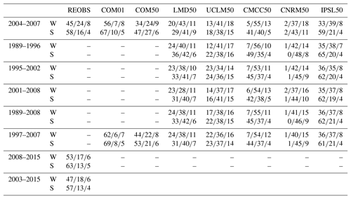
Table 4 presents an estimate of the frequencies of occurrence of nonprecipitating days, very light precipitation and light precipitation for winter (Julian day 1 to 100) and summer (Julian day 151 to 251) when considering either the common period of the two datasets (2004–2007) or the full period of each dataset (i.e., 1997–2007 for COMEPHORE and 2003–2015 for SIRTA rain gauge). The number of dry days increases for the two estimations from COMEPHORE when considering a longer period than the common period. For ReOBS, the statistics remain similar for the two different periods. However, when considering the most recent years only, which will be used in the next section (2008–2015), the number of dry days increases. The influence of the number of years, the years considered and the products used to estimate these frequencies of occurrences is generally small but significant. Even though model errors are most of the time beyond this uncertainty, it has to be kept in mind in the following analysis.

3.3 Method to establish the relationship between IWV and precipitation as a function of tropospheric temperature

The objective is to characterize how precipitation depends on IWV for different ranges of mean tropospheric temperature. To do that, we divided our datasets into four different bins of temperature: the first bin is for temperature less than or equal to 254.5 K, the second bin is for temperature between 254.5 and 258 K, the third one corresponds to temperature between 258 and 262.5 K and the fourth one is for temperature higher than 262.5 K. This choice has been made to ensure a high number of samples in each bin of temperature to proceed to the next step. In this way, the mean tropospheric temperature of one bin is similar more or less 1 K for all the datasets. Then, in each bin of temperature, the daily mean precipitation rates are sorted according increasing values of daily mean IWV. IWV bins are then defined such that they contain an equal number of pairs of precipitation rates and IWV (40 samples) to ensure a reasonable number of days to compute the 50th quantile of precipitation, which indicates if there are more precipitating days than nonprecipitating days. The range of each IWV bin is thus not constant but allows the transition between mostly nonprecipitating days and mostly precipitating days to be identified quite easily. For each model and for observations, a critical value of IWV (w_c) is then determined for each different bin of temperature by using a very simple algorithm. This one identifies the value(s) of IWV over which the 50th quantile of precipitation is greater than 0.1 mm day⁻¹. In some cases, two values are obtained, which are represented by an error bar to indicate the uncertainty of the estimate of this critical value.

4 Humidity biases in the Med-CORDEX simulations

4.1 Comparison with GPS dataset at regional scale

Figure 1 indicates the mean values of IWV retrieved from GPS measurements in winter (Fig. 1a) and in summer (Fig. 1b). In winter, higher values are observed along the Atlantic and Mediterranean coasts while central and eastern Europe exhibit very low values of IWV. In summer, there are two different regimes: (i) north of 45^∘ N showing a decrease in IWV values while going to Scandinavia, following the temperature gradient; (ii) around the Mediterranean, the structure is more patchy with alternating low and high values. Most low values correspond to higher topography but not systematically.

Table 3 shows the mean bias and the standard deviation (SD) of ERA-Interim and RCMs' IWV on their native grid or regridded to ERAI grid, in comparison to GPS estimates. Daily datasets are used to compute these statistics and exactly the same sampling is used between models and observations. It shows that the mean bias ranges from 0.5 to 1.0 kg m⁻² except for CNRM50 and UCLM50, for which the biases are stronger (up to 1.8 kg m⁻² for UCLM50 on its native grid). It is to be noted that the mean biases are generally not better on the native grid (50 km resolution) than when regridded on the ERAI grid (75 km resolution). The correction of topography improves the comparison for all models but ERAI and LMD50 on its native grid.

The standard deviation indicates a large spread around observations for all models (∼3.5 to 4.0 kg m⁻²), except IPSL which is even better than ERA-Interim. The nudging towards ERA-Interim used in this simulation likely explains this behavior. This large standard deviation, which is reduced when using the corrected topography, does not mean that the model is wrong in a climatological context, but it is the result of internal variability in the absence of nudging, generating deviations from its driving data in the interior of the domain (e.g., Kida et al., 1991), partly compensated for by potential artificial flows created to achieve physical consistency with the lateral boundary conditions (Becker et al., 2015; Omrani et al., 2015). However, in the configuration of Med-CORDEX, the domain is quite small and the jump of resolution between lateral boundary conditions (75 km) and the RCM (50 km) is also weak, so that we could have expected smaller differences between a model using nudging and a model not using nudging (Matte et al., 2017).

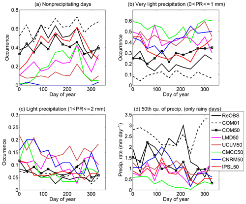
Figure 2 Occurrence for 30-day periods from January to December over the years 2004–2007 of (a) nonprecipitating days; (b) precipitation rates between 0 and 1 mm day⁻¹; (c) precipitation rates between 1 and 2 mm day⁻¹. (d) Value of the 50th quantile of precipitation (excluding nonprecipitating days). Each color corresponds to a different model at 50 km resolution regridded to the LMD grid (see legend for details). Black line is for observations at SIRTA supersite (ReOBS). Dashed black line is for COMEPHORE product at 1 km × 1 km resolution at the closest grid point of SIRTA (COM01) and black line with squares is for COMEPHORE averaged over a square of 50 km × 50 km around SIRTA (COM50).

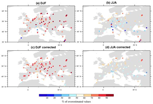
Figure 3 Percentage of simulated daily mean IWV values which overestimate the GPS ones (a) in winter and (b) in summer. Simulated values are taken from five models at 50 km resolution (LMD50, IPSL50, CNRM50, CMCC50, UCLM50) regridded to the ERAI grid. Panels (c) and (d) are the same as (a) and (b) but for height-corrected values.

To the first order, the IWV variability is dominated by the seasonal cycle (shown in Fig. 1), which is underestimated by models (not shown), and which explains part of the model standard deviation: indeed, Fig. 3 shows the percentage of simulated daily mean IWV values which overestimate GPS values at each station for the ensemble of the five models regridded to the ERAI grid, in winter and summer. Figure 3a and b present results without height correction, while Fig. 3c and d are done with height-corrected data. In winter, more than 70 % of values are overestimated over most stations, with or without height corrections. In summer, this percentage decreases appreciably in most stations and in almost half of them it reaches values below 50 % (Fig. 3b). The use of height correction homogenizes the results in summer between stations and the very low or very high percentages do not appear anymore when this correction is applied. UCLM50 simulation is the moistest, especially in summer (not shown), which explains its high standard deviation in Table 3.

The IWV variability also comes from the interannual variability. For each month, we computed its anomaly by subtracting the average value of the month over all the years. We then computed the correlation between the anomalies of the GPS IWV estimates and those from the models. The minimum and maximum values of these correlations for each model when all stations are considered are indicated in Table 3 (last column). As indicated by these numbers that range between 0.78 and 0.99, the interannual variability is captured well by the model, which is not surprising since this variability is mostly driven by large-scale advection of air masses (all models use 6-hourly ERA-Interim parameters as lateral boundary conditions). Note that the maximum correlation is very high for all models, while the minimum values are higher for ERAI, LMD50 and IPSL50 than for the three others. This is mostly due to a specific month (not shown): in January 1996, three models have an anomaly very different from the observations and, as a consequence, the interannual correlation for January goes down.

To conclude, the RCM configuration allows a reasonable representation of the large-scale advection of air masses by the models, which is an important driver of humidity within the RCM domains (see also Trenberth et al., 2005). This is further improved when the model is nudged towards reanalysis, as in the IPSL model (Table 3).

Nevertheless RCM errors are significant, with a difficulty in reproducing low values of IWV, generating a mean positive bias for all models. Most of the contribution of humidity to the integrated water vapor comes from the surface, and the interaction between environment and clouds and boundary layer. Small-scale processes are thus important to reproduce moisture sources and sinks (precipitation, mesoscale circulations, evaporation and evapotranspiration, clouds and microphysics). To better understand these errors, we assess the link between surface humidity and IWV at different timescales. Figure 4 displays the monthly mean values of IWV versus monthly mean values of 2 m specific humidity (Q2) averaged over all stations where and when both IWV from GPS and Q2 from HadISD are available. Monthly means are computed if at least 60 concomitant (both IWV from GPS and Q2 from surface station) values are available (i.e., about two values per day out of a possible four). A total of 3238 months are obtained, spread over 42 different stations. The average number of stations per month is 19 with a maximum of 30 stations. Figure 4 shows that 2 m specific humidity is a very good proxy for IWV at the monthly scale. All models but IPSL have a similar relationship between the two variables to the observed one (slope of 2.4×10³ kg m⁻²). However, for a given surface humidity, IWV is generally overestimated by models, especially for the driest conditions. The IPSL model presents a different behavior: for low values of surface humidity, IPSL shows the same bias as the other models, while at higher Q2 values, its bias strongly increases, generating a different regression slope than observations. IPSL compensates its underestimation of surface humidity in summer (Bastin et al., 2018) by a steeper slope. This compensation may be the result of the use of nudging or it can be due to a deep boundary layer so that the total humidity contained within the boundary layer is similar to that of other models (not possible to check that). Since the nudging is only used above the boundary layer, and since most of the humidity is contained within the boundary layer, there is little reason that the nudging totally explains this compensation. It means that for this model, Q2 is not a good proxy of total column humidity, even at monthly scales. Note also that the spread between models is a bit higher in summer than in winter, most probably because of more active boundary layers and increased entrainment of humidity from the free troposphere at their top. These processes will also affect the link between surface humidity and IWV at scales shorter than a month.

Table 5 Summertime interannual correlation between IWV and Q2 at GPS stations. In bold, the mean value for each model, followed by min and max values. The other values in the table corresponds to the standard deviation of the difference in correlation between two models.

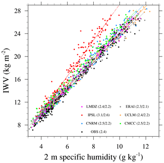
Figure 4 Monthly values of IWV as a function of monthly values of 2 m specific humidity (Q2) averaged over all stations where and when both IWV from GPS and Q2 from HadISD are available. Monthly means are computed if at least 60 coexisting values exist (i.e., about two values per day over a possible four). A total of 3238 months are obtained, spread over 42 different stations. The average number of stations per month is 19 with a maximum of 30 stations). The color of circles corresponding to each model is indicated on the legend. All model outputs have been regridded to the ERAI grid. The first number indicates the slope of the regression obtained when considering the same months than observations at each station, while the second number is the slope of the regression when considering all months at all grid points (only models).

Despite the strong correlation between the annual cycle of Q2 and those of IWV, Q2 is not necessarily a good proxy for IWV at other timescales or to tackle model biases (for instance IPSL bias for surface humidity is strongly negative while it is weak and slightly positive for IWV). While in the wintertime, humidity variability mostly originates from the air mass advection, summertime variability is mainly affected by land–surface interactions and boundary layer processes. Several studies have shown the existence of a large spread in the representation of the surface fluxes and land–atmosphere coupling strength between models over Europe, due to the fact that Europe is a zone of transition between the regime of “energy-limited” areas with low land–atmosphere coupling strength and those of “oil-moisture-limited” areas with high land–atmosphere coupling strength. The difficulty to represent soil conditions and surface fluxes is then increased (Cheruy et al., 2015; Boe and Terray, 2014; Fischer et al., 2007; Knist et al., 2017). The interannual correlations between IWV and Q2 summertime anomalies are indicated for each model in Table 5, as averaged values over all GPS stations and minimum and maximum values across all GPS stations (an attempt was made for GPS IWV and HadISD Q2 but there were too many missing values). For most stations, the correlation is higher than 0.5 with a mean value around 0.8 for the five models. The standard deviation of the difference between models is around 0.15, which reveals a good agreement between them. Some stations, however, indicate higher differences, as indicated by the minimum values that strongly differs between models. IPSL50 and LMD50 models present strong correlation at all stations (r > 0.52 and 0.43, respectively) while it is very weak at some stations for UCLM50, CNRM50 and ERAI. It can be explained by a stronger availability of surface humidity in summer, and then a weaker sensitivity of IWV to the surface moisture availability. For the drier models (e.g., IPSL50), a dry interannual anomaly of soil moisture will have an impact on the surface evaporation and then on the IWV anomaly. On the other hand, over areas where the advection of air masses from the sea or ocean is a more important driver, the interannual variability of the large-scale dynamics affects both IWV and surface humidity more strongly than surface processes. Depending on the area and on the model, Q2 and IWV thus convey different but complementary information about the model behavior.

4.2 Scaling of IWV with temperature

A way to check the behavior of models is to consider the relationship between IWV and temperature. At global scale, the scaling of IWV with temperature is expected to follow the Clausius–Clapeyron (C-C) law, at a rate of about 6 % ^∘C⁻¹ to 7 % ^∘C⁻¹. At regional scale, this relationship deviates from C-C due to the strong influence of dynamics (air mass advection) and moisture availability (e.g., Drobinski et al., 2016). Figure 5a illustrates the scaling of IWV with temperature over the SIRTA station, which is representative of most stations over Europe. For the lower temperature, the scaling follows the C-C law. Above a critical temperature (T_break), IWV stops increasing at this rate. This critical temperature, defined as the temperature when the slope of the relationship deviates from C-C, presents spatial variations that are displayed in Fig. 5c for observations. For most stations, the critical value is between 15 and 18 ^∘C. It is higher for stations located around the Mediterranean Sea, the Black Sea or at the eastern edge of the domain, in the Dnieper and Volga basins. The IWV value corresponding to this critical temperature (which is close to the maximum IWV value reached at each station) is more variable (Fig. 5d), due to a combined effect of T_break value, orography and latitudinal differences.

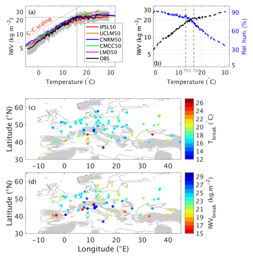
Figure 5 (a) IWV–T(2 m) relationship at SIRTA station from observations and models. Median values are plotted for observations and models. The grey band represents the interval between the 20th and 80th quantiles for observations. The black vertical dashed line shows T_break, the black horizontal dashed line shows IWV_break, and the red slant dashed line shows C-C scaling. (b) Median values of IWV and RH(2 m) as a function of T(2 m) at SIRTA from observations only. The vertical grey dashed lines indicate the values of Tb1 and Tb2 (see Sect. 4). (c) Map of T_break at all the GPS stations. (d) Map of IWV_break at all the GPS stations.

Physically, T_break corresponds to the value when the relative humidity significantly decreases due to a lack of humidity sources.

To determine the slope after T_break, we can approximate the expression of IWV:

$${\displaystyle }\mathrm{IWV}\left(T\right)={\int }_{z=\mathrm{0}}^{z=\mathrm{TOA}}{\mathit{\rho }}_{\mathrm{v}}\left(T,z\right)\mathrm{d}z=-{\displaystyle \frac{\mathrm{1}}{g}}{\int }_{{\mathrm{P}}_{\mathrm{s}}}^{P_{\mathrm{TOA}}}Q\left(T,P\right)\mathrm{d}P,$$

with Q the specific humidity at altitude z, ρ_v the density of water vapor in kilograms per cubic meter (kg m⁻³), P_s the surface pressure and P_TOA the pressure at the top of the atmosphere (TOA).

As observed (e.g., Ruzmaikin et al., 2014), on average the troposphere can be separated into two layers, one being the boundary layer (BL) and the other one the free troposphere (FT) – assuming constant humidity within the two layers, IWV can be expressed as follows:

$$\begin{array}{ll}{\displaystyle }\mathrm{IWV}\left(T\right)& {\displaystyle }\approx {\displaystyle \frac{\mathrm{1}}{g}}(\left(P_{\mathrm{s}}-P_{\mathrm{BL}}\right)\times Q_{\mathrm{BL}}\left(T_{\mathrm{BL}}\right)+\left(P_{\mathrm{BL}}-P_{\mathrm{TOA}}\right)\\ {\displaystyle }& {\displaystyle }\times Q_{\mathrm{FT}}\left(T_{\mathrm{FT}}\right)).\end{array}$$

P_s is about 1000 hPa, P_TOA between 0 and 10 hPa, and P_BL around 800–850 hPa, so that we can write the following:

$${\displaystyle }(P_{\mathrm{s}}-P_{\mathrm{BL}})=\mathit{\alpha }(P_{\mathrm{BL}}-P_{\mathrm{TOA}})\cong \mathit{\alpha }{P}_{\mathrm{BL}}.$$

For an air mass at temperature T and specific humidity Q, we can write Q(T)= RH ×Q_s(T), with subscript s for saturation and RH for relative humidity, which gives the following:

$$\begin{array}{ll}{\displaystyle }\mathrm{IWV}\left(T\right)& {\displaystyle }\approx {\displaystyle \frac{\mathrm{1}}{g}}\left(\mathit{\alpha }{P}_{\mathrm{BL}}\times {\mathrm{RH}}_{\mathrm{BL}}\times Q_{\mathrm{s}}\left(T_{\mathrm{BL}}\right)+P_{\mathrm{BL}}\times {\mathrm{RH}}_{\mathrm{FT}}\right.\\ \text{(1)}& {\displaystyle }& {\displaystyle }\left.\times Q_{\mathrm{s}}\left(T_{\mathrm{FT}}\right)\right).\end{array}$$

With our simplified profile in two layers, we have Q_s(T_FT)≈αQ_s(T_BL) if we consider that T_BL is around 280–290 K (Q_s then ranges between ∼6 and ∼12 g kg⁻¹ according to the August–Magnus–Roche formula) and T_FT around 260 K (for T < 260 K, the value of T does not affect the value of Q^s much since it has nearly reached its minimum value, being inferior to 2 g kg⁻¹).

RH_FT can approximately be considered as a constant, close to 30 % in average over Europe (Ruzmaikin et al., 2014)

Equation (1) can thus be approximated by the following:

$${\displaystyle }\mathrm{IWV}\left(T\right)\approx {\displaystyle \frac{\mathit{\alpha }}{g}}{P}_{\mathrm{BL}}\left({\mathrm{RH}}_{\mathrm{BL}}+{\mathrm{RH}}_{\mathrm{FT}}\right)\times Q_{\mathrm{s}}\left(T_{\mathrm{BL}}\right).$$

And finally, by differentiation we obtain Eq. (2):

$$\begin{array}{}\text{(2)}& {\displaystyle \frac{\mathrm{1}}{\mathrm{IWV}}}{\displaystyle \frac{\partial \mathrm{IWV}}{\partial T}}\approx {\displaystyle \frac{\mathrm{1}}{Q_{\mathrm{BL}}^{\mathrm{s}}}}{\displaystyle \frac{\partial Q_{\mathrm{BL}}^{\mathrm{s}}}{\partial T}}+{\displaystyle \frac{\mathrm{1}}{{\mathrm{RH}}_{\mathrm{BL}}+{\mathrm{RH}}_{\mathrm{FT}}}}{\displaystyle \frac{\partial {\mathrm{RH}}_{\mathrm{BL}}}{\partial T}}.\end{array}$$

The first term of the right-hand side (RHS) of Eq. (2) is the variation in the water-holding capacity of the atmosphere at temperature T and is thus the Clausius–Clapeyron rate (∼7 % C^∘−1 at 25 ^∘C).

Table 6 Values of the left-hand side (LHS), second term of the right-hand side (RHS) and total RHS of Eq. (2) computed for the SIRTA site for two different temperatures (10 and 20 ^∘C), according to Fig. 5d for observations and Fig. 6a for models.

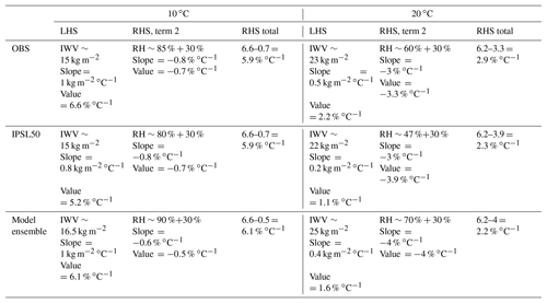
At temperatures lower than T_break, RH is nearly constant, so that the second term of RHS of Eq. (2) is close to zero and the slope of IWV as a function of temperature follows C-C. According to Eq. (2), the deviation of the slope from C-C after T_break should correspond more or less to the rate of RH decrease, which depends on the considered station. Figure 5b shows RH and IWV as a function of T for SIRTA observations. RH starts to decrease significantly at T∼13 ^∘C (hereafter called T_b1), while the IWV curve is deflected at T∼16 ^∘C (hereafter called T_b2). Table 6 indicates the values of the left-hand-side term of Eq. (2) and the second term of the right-hand side of Eq. (2) before T_b1 (at 10 ^∘C) and after T_b2 (at 20 ^∘C). In spite of the important approximations done to obtain Eq. (2), the RH variations in the boundary layer thus explain to the first order the scaling of IWV with T. The determination of humidity sources that explain the RH variability are thus crucial.

Figure 5a indicates that despite the bias at low temperature, models generally capture the deviation from C-C and the IWV maximum value that is reached at high temperature, except for the UCLM model for which IWV continues to increase slightly with T. Note that the model slopes at low T are a bit lower than that of the C-C law and that derived from the observations. They are also often slightly different above the critical value, indicating some difficulties in simulating the relative humidity decrease. Figure 6a shows the model ensemble mean of the scaling at the SIRTA station. It confirms that the deviation from C-C exists but the transition is smoother in the models than in the observations which makes the estimate of T_break more uncertain at this station. However, some stations show more abrupt transitions (not shown). For the ensemble, due to the smooth transition, T_break is thus defined as the temperature value when IWV stops increasing (i.e., when it reaches its hiatus value). Figure 6b and c indicate the model ensemble mean value of T_break and the corresponding IWV_break. The models capture the spatial pattern of T_break, especially the higher values close to the Mediterranean, the Black Sea and in the eastern edge of the domain, but tend to overestimate it compared to the observations (Fig. 5c) but as already said, the uncertainty on the T_break estimate is quite high. The maximum value of IWV is also generally well simulated by the models, except over the northern part of the domain where the UCLM50 simulation does not always capture this break (as seen in Fig. 5a), indicating an overestimation of relative humidity.

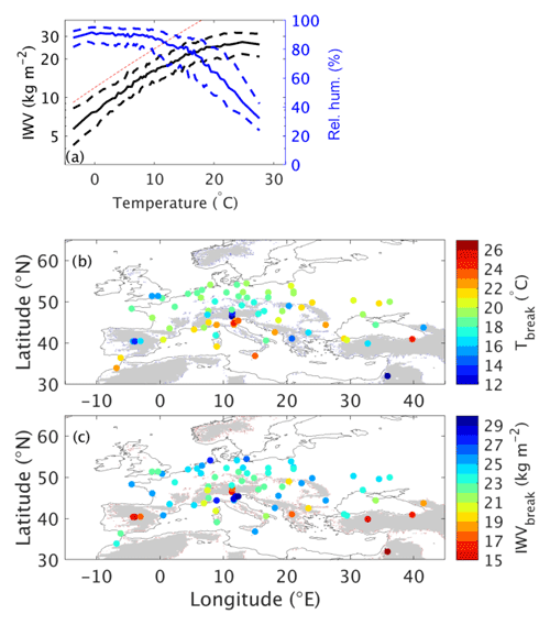
Figure 6 (a) Scaling of IWV (black) and RH (blue) with temperature for the model ensemble at SIRTA station. Solid lines are for quantile 50 and dashed lines are for quantiles 20 and 80 of the distributions. The red slant dashed line shows C-C scaling. Panels (b) and (c) are as in Fig. 5c, d but for the model ensemble.

The link between the IWV and RH evolutions for the model ensemble is shown in Fig. 6a. Once again, the transition from one regime to another is smoother than for observations (Fig. 5b), but the decrease in RH starts around the same range of temperature as for the transition of IWV–T relationship. Table 6 confirms that in model RH variations in the boundary layer also explain to a good degree the scaling of IWV with T.

In conclusion to this section, models tend to overestimate low values of IWV. Although they generally capture the IWV scaling with temperature well, small-scale processes also explain part of the standard deviation (not only induced by the deviations from driving data) when considering the differences with GPS IWV data. In the next section, we consider the impact of these humidity biases in models of light precipitation occurrence.

5 Impact of model biases on light precipitation

5.1 Over SIRTA

Figure 7 displays the 50th percentile of precipitation (computed including days without precipitation) as a function of IWV for four different bins of mean tropospheric temperature for both observations and the models (see Sect. 3 for the details of the methodology). The observations are considered for the period 2008–2015 and the different models for the period 2001–2008 (i.e., the same number of years, despite the time shift). For all these datasets, there exists a critical value of IWV, w_c, over which precipitation starts to increase. The values of these critical values are determined from Fig. 7 following the methodology indicated in Sect. 3.3. The critical value depends on temperature (it increases with temperature) and on the models, as shown in Fig. 8a. UCLM50 presents lower critical values of IWV than observations at all temperatures, and also CNRM50 at high temperatures. This means that in these models the precipitation begins in a drier atmosphere than that which begins to produce rain in the observations. On the contrary, for CMCC50, at high temperature, the atmosphere needs to be as wet or wetter than what is observed to trigger precipitation. IPSL50 and LMD50 present similar values than observations for this critical value. CNRM50 and UCLM50 are the two models, which present light precipitation too often and not enough days without precipitation (Fig. 2).

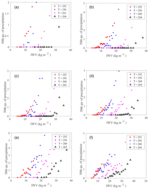
Figure 7 The 50th quantile of precipitation as a function of IWV for four different bins of tropospheric temperature at 48.7^∘ N, 2.2^∘ E (SIRTA). (a) SIRTA-ReOBS observations. (b) CMCC50. (c) IPSL50. (d)  LMD50. (e) CNRM50. (f) UCLM50. Observations are analyzed for the period 2008–2015, and models for the period 2001–2008. The values of T indicated in the legends correspond to the mean values in the bins that have been chosen as indicated in the text.

The second reason for the high frequency of occurrence of very light precipitation in these models is that the probability of exceeding this critical value of IWV is strongly overestimated in these two models in comparison with observations (Fig. 8b). Statistically speaking, it means that the models that are too humid have a positive bias in light precipitation. For CMCC, the dipole between winter and summer observed in the estimate of nonprecipitating days is also observed here: though the critical value of IWV is correct at low and moderate T, the probability of exceeding it is too strong, i.e., typically during winter, which explains why it rains too much during winter, while it is not the case during summer, with very low probability of exceeding the high critical value of IWV. IPSL model is dry both in terms of humidity and precipitation, and LMD50 follows observations but with a slightly higher probability of exceeding the critical value. It is also important to note that the underestimation of nonprecipitating days for all models in winter is consistent with the systematic overestimation of low values of IWV (Figs. 3, 4, 5).

Table 7 Period for which the maximum value of the temperature bin (T) and the critical value of IWV (w_c) is reached. Period 1 is for 1989–1996, P2 for 1995–2002 and P3 for 2001–2008. The second number in the column of w_c corresponds to the maximum relative variability of IWV computed as ((max(w_c)-min(w_c))/mean(w_c)) for each temperature bin and each model.

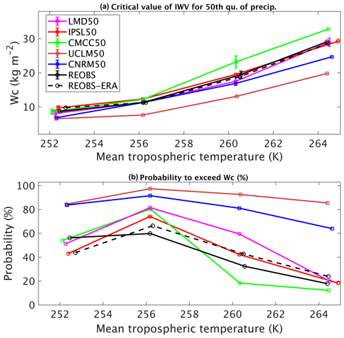
Figure 8 (a) Critical value of IWV at 48.7^∘ N, 2.8^∘ E over which 50th quantile precipitation significantly increases as a function of the mean tropospheric temperature. Each color corresponds to a different model (see legend for details). The period considered is 2001–2008. Solid black line is for observations from the SIRTA-ReOBS dataset between 2008 and 2015 and dashed black line is for SIRTA-ReOBS with ERA-Interim tropospheric temperature instead of tropospheric temperature from radiosoundings. (b) Probability of IWV exceeding the critical value for each dataset.

In addition to the period 2001–2008 discussed above, we tested two other 8-year periods (1989–1996 and 1995–2002) and the entire period (1989–2008) to assess the influence of the considered period on the results. Figure S1 in the Supplement and Table 7 show that results are rather robust among models and periods, though some uncertainty exists in both w_c and the probability of exceeding it. The maximum relative variability in w_c for one model is around 25 %, which is small compared to the maximum difference when considering all values from all models that is 58 % for bin 1 (253 K), 73 % for bin 2 (257 K), 63 % for bin 3 (261 K) and 64 % for bin 4 (264 K). The warming of the tropospheric temperature due to climate change is also visible in Fig. S1 and in Table 7 since for all models and for the three warmer temperature bins, the warmer temperature is obtained during the most recent period (2001–2008; i.e., period 3). On the contrary, lower temperatures (first bin) tend to decrease, indicating a tendency of the distribution to become wider. We can note that due to the variability of the critical value of IWV and the variability of T inside each bin, the maximum value of w_c inside each bin is not always obtained during the period of maximum temperature. For the first bin, four models out of six indicate a higher value of w_c during the first period, which is the warmer for this bin. For the other three bins, the maximum temperature is obtained for all six models during the most recent period, i.e., period 3 (100 % of values), while this period gets only 39 % (7 out of 18 cases) of maximum w_c values, and the three other periods represent about 20 % each.

Table 8 Latitude/longitude/altitude (^∘/^∘/m) of the closest grid point of each model for the GPS stations used.

5.2 Generalization

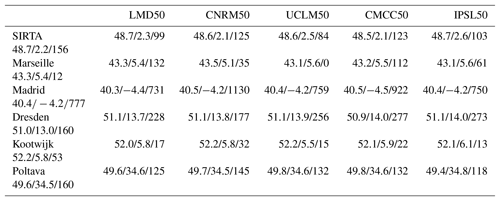
To have an idea of the models' behavior over other parts of Europe, several other stations are considered in this section. Their locations are shown in Fig. 1b by black diamonds and details are given in Table 8. Except for Marseille located in the south of France where the COMEPHORE product associated with GPS has been used, the model outputs are not compared with observations for the other stations. Figure 9 displays the occurrence of nonprecipitating days for the different models and from the COMEPHORE product at the station location when available (over France), w_c values as a function of temperature and the percentage of IWV values that exceed w_c as a function of temperature. The observed frequency of occurrence of nonprecipitating days is slightly higher in Marseille, located in the dry southern France, than in the northern part of France (SIRTA). Most of the models (except CNRM50) overestimate this north–south gradient. For instance, for UCLM50, the frequency is between 80 % and 90 % at Marseille, while it is around 15 % at SIRTA. Several other characteristics of the models' behavior do not depend much on the station: CNRM50 always simulates less occurrence of nonprecipitating days than other models and simulates a rather flat annual cycle; the annual cycle simulated by CMCC50 is always very intense, with a much higher frequency of occurrence of nonprecipitating days in summer than in winter, and IPSL is always the model with the highest frequency of occurrence of nonprecipitating days; UCLM50 and LMD50 are between CNRM50 and IPSL50, with a tendency to simulate many days with very light precipitation at the northern stations (Figs. 2 and 9g, m) but not at the southern ones (Fig. 9a, d). In the eastern part of the domain (Fig. 9j), the annual cycle of precipitation simulated by models is a bit different than elsewhere, with two drier periods in spring and fall.

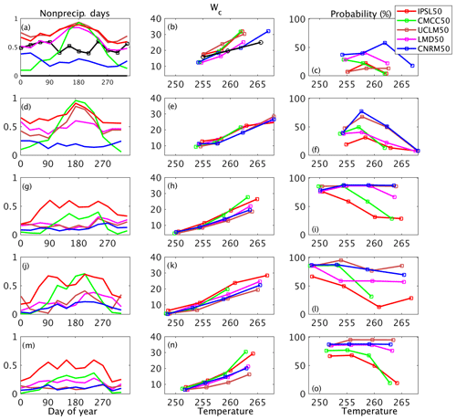
Figure 9 (a, d, g, j, m) Annual cycle of occurrence of nonprecipitating days for the different models and COMEPHORE in black in panel (a) (same legend as Fig. 8 for models). (b, e, h, k, n) Value of w_c (maximum value) as a function of tropospheric temperature. (c, f, i, l, o) Probability of exceeding w_c value. First row is for the station located in southern France (Marseille), second row for the one located in central Spain (Madrid), third row for the station in eastern Germany (Dresden), fourth row in Ukraine, and fifth row in the Netherlands (see Table 8 and Fig. 1 for details on the locations of the stations).

To relate these characteristics to temperature and humidity, we reproduced the analysis done at SIRTA. The value of the critical value of IWV over which precipitation starts to increase is generally similar among models, despite increasing dispersion with temperature. This value depends on the stations, indicating the influence of local specificities in the estimation of this relationship. For instance, UCLM50, which is the model with the most important difference between southern and northern stations for the annual cycle of dry days, also indicates strong differences in the w_c for a similar temperature, with a critical value around 25 kg m⁻² in Marseille for a tropospheric temperature of 260 K (Fig. 9b), while it is ∼12 kg m⁻² in the Netherlands (Fig. 9n). The nature of precipitation, more or less convective, likely explains these differences. The probability of exceeding the critical value is the most discriminant parameter between models and between seasons. Results are robust and confirm the importance of the relationship between temperature, IWV and light precipitation: for a given bin of temperature if the model is too humid (higher probability of exceeding the threshold), it rains too often.

6 Conclusions

This work uses GPS integrated water vapor measurements associated with temperature and precipitation measurements to (i) estimate the biases of six regional climate models over Europe in terms of humidity; (ii) understand their origins; and (iii) finally assess the impact of these biases on the occurrence of precipitation.

The first part of the study aimed at evaluating the mean bias and standard deviations of IWV in models compared to GPS measurements at interannual, seasonal and daily timescales. An interesting result is that all models overestimate the lower values of IWV (nighttime, wintertime) at all stations. The spread among models is increased during summertime. Our analysis suggests that the model physics mostly explain the mean biases, while dynamics affects the variability. The use of nudging towards reanalyses thus improves the representation of the large-scale advection of air masses and reduces the standard deviation of differences between GPS retrieved IWV values and simulated ones. The land surface–atmosphere interactions are crucial in the estimation of IWV over most part of Europe, especially in summer, and explain part of the mean biases. However, the relationship between IWV and temperature, which deviates from the Clausius–Clapeyron law after a critical value of temperature, is generally well captured by models. This critical temperature presents a spatial variability since it corresponds to the value when relative humidity starts to decrease. It is thus strongly dependent on local processes which drive the local humidity sources (from evaporation and advection). This explains why the maximum values of IWV are not necessarily observed over warmer areas, which often corresponds to dry areas, where a soil-moisture-limited regime is dominant.

The improvement in humidity representation may also help in the representation of precipitation distribution. Indeed, in the second part of this study, it is shown that the biases in IWV and most importantly IWV's distributions as a function of temperature strongly impact the occurrence of light precipitation over France, and most generally over areas where convection is the main process of precipitation triggering. For each range of mean tropospheric temperature, there exists a critical value of IWV over which a pickup in precipitation occurs. This is observed and simulated by models, but the critical values and the probability of exceeding them vary between models and observations. Models which present light precipitation too often generally show lower critical values and higher probability of exceeding them. Thus, a better knowledge and representation of the triggering thresholds of precipitation and of their variability should potentially help to improve the representation of the whole precipitation distribution in models. The ensemble of simulations with implicit and explicit convection that will be performed in the framework of the Flagship Pilot Studies' convective-permitting climate simulation of the CORDEX project will allow us to assess the sensitivity of precipitation triggering and distribution to the model resolution. Issues that will be explored in more detail following this work will be the role of humidity in (i) the triggering of precipitation in simulations at different resolution, (ii) the low precipitation rates (precipitation efficiency) and (iii) the impact of too-easy triggering in the entire precipitation distribution.