Source attribution of European surface O₃ using a tagged O₃ mechanism

Tropospheric ozone (O₃) is an important air pollutant that affects human health, ecosystems, and climate. The contributions of O₃ precursor emissions from different geographical source regions to the O₃ concentration can help to quantify the effects of local versus remotely transported precursors on the O₃ concentration in a certain area. This study presents a “tagging” approach within the WRF-Chem model that attributes O₃ concentration in several European receptor regions to nitrogen oxide (NO_x) emissions from within and outside of Europe during April–September 2010. We also examine the contribution of these different precursor sources to various O₃ metrics and their exceedance events. Firstly, we show that the spatial distributions of simulated monthly mean MDA8 from tagged O₃ source regions and types for late spring, summer, and early autumn 2010 varies with season. For summer conditions, O₃ production is dominated by national and intra-European sources, while in the late spring and early autumn intercontinental transported O₃ is an important contributor to the total O₃ concentration. We have also identified shipping activities in the Mediterranean Sea as an important source of O₃ for the Mediterranean countries, as well as the main contributor to high modelled MDA8 O₃ concentration in the Mediterranean Basin itself. Secondly, to have a better understanding of the origin of MDA8 O₃ exceedances, we compare modelled and observed values of MDA8 O₃ concentration in the Po Valley and Germany–Benelux receptor regions, revealing that the contribution from local sources is about 41 % and 38 % of modelled MDA8 O₃ during the exceedance days, respectively. By examining the relative contributions of remote NO_x sources to modelled and observed O₃ exceedance events, we determine that model underrepresentation of long-range O₃ transport could be contributing to a general underestimation of modelled O₃ exceedance events in the Germany–Benelux receptor region. Thirdly, we quantify the impact of local vs. non-local NO_x precursors on O₃ production for each European receptor region using different O₃ metrics. The comparison between mean, MDA8 and 95th percentile O₃ metrics accentuates the importance of large contributions from locally emitted NO_x precursors to the high end of the O₃ distribution. When we compare the vegetation and health metrics, we notice that the SOMO35 and AOT40 indexes exhibit rather similar behaviour, while the W126 index accentuates the importance of local emissions. Overall, this study highlights the importance of a tagging approach to quantify the contribution of local and remote sources to the MDA8 O₃ concentration during several periods as well to different O₃ metrics. Moreover, this method could be applied to assess different mitigation options.

1 Introduction

Tropospheric ozone (O₃) is formed primarily during the oxidation of volatile organic compounds (VOCs) in the presence of nitrogen oxides (NO_x) and sunlight. Ground-level O₃ is an important air pollutant that damages human health (Fleming et al., 2018) and vegetation (Mills et al., 2018). It also affects the radiative forcing (e.g. Ramaswamy et al., 2001; Stevenson et al., 2013) and therefore contributes to climate change. Impacts of O₃ on human health are associated with lung disease, chronic disease, and death from respiratory ailments. To protect human populations from exposure to high levels of O₃, the World Health Organization (WHO, 2006, 2017) recommended an air quality guideline for ozone in which the maximum daily average 8 h (MDA8) for O₃ should not exceed 100 µg m⁻³. The European Environmental Agency (EEA, 2017a) reported that the EU long-term objective target concentration of 120 µg m⁻³ is often exceeded and that more than 90 % of the urban population of the European Union was exposed to O₃ levels higher than the stricter recommendation set by the WHO. A 2010 report from HTAP (HTAP, 2010) shows that the observed baseline O₃ concentrations (concentrations without the contribution from local anthropogenic emissions) have increased throughout the last several decades since overall global anthropogenic emissions of O₃ precursors have increased. However, a more recent study by Gaudel et al. (2018) has established that the global surface O₃ trends exhibit high variability and depend on several factors such as season, region, elevation, and proximity to fresh ozone precursor emissions. However, since the network capable of monitoring ozone levels is sparse, it is difficult to quantify the O₃ changes on a global scale. Satellite-derived O₃ measurements can be used to quantify changing levels of O₃, but Gaudel et al. (2018) showed that these products are not capable of quantifying significant trends. Surface O₃ pollution due to urbanisation and motorisation processes are serious challenges for large cities (e.g. Chan and Yao, 2008; Folberth et al., 2015; Li et al., 2017, 2019). Paoletti et al. (2014) showed that in Europe and the United States of America, the average O₃ concentration in the cities has increased at a faster rate than that observed in rural areas. Fleming et al. (2018) showed that the fourth highest daily maximum 8 h O₃ (4MDA8) is more ubiquitous at urban sites than at non-urban sites. This leads to a worsening of general air quality that, ultimately, affects human health and ecosystems (Paoletti et al., 2014; Monks et al., 2015; WHO, 2017; Fleming et al., 2018; Mills et al., 2018). To improve the air quality in certain areas, it is important to know the extent to which different precursors (NO_x and VOCs) contribute to tropospheric O₃ concentrations.

Information regarding levels of NO_x and VOC emissions and weather conditions enhances our ability to predict the formation of tropospheric O₃. The continuous development of chemical transport models can lead to a better understanding of the processes that contribute to high-O₃ episodes. Knowing the impacts of NO_x and VOC emissions from sources such as surface anthropogenic activities, fires, soil, and the stratosphere on total O₃ production can help authorities develop strategies aimed at reducing the impact of high levels of O₃ on the well-being of both humans and ecosystems. Several approaches have been used to determine the extent to which individual sources contribute to total levels of O₃. For example, perturbation of different emission categories has allowed scientists to make estimations regarding the contributions of individual sources of O₃ to total O₃ levels (e.g. Fiore et al., 2009).

Tagging techniques have also been used in modelling studies to determine source–receptor relationships and how individual sources of pollutants contribute to total pollution levels at given locations. Pollutants with relatively low chemical reactivities, such as carbon monoxide (CO), can be “tagged” according to their emission sectors or regions for attribution studies (e.g. Pfister et al., 2011). Sudo and Akimoto (2007) and Derwent et al. (2015) used O₃ tracers tagged by their region of formation to show that intercontinental transport of O₃ can occur from polluted source regions, such as North America and East Asia, and appears to be the most important source of tropospheric O₃ in Europe. Other studies, including those of Wang et al. (2009) and Grewe et al. (2010, 2012, 2017), have used tagging methods to identify the contribution of individual sources of O₃ to overall levels. This method is especially useful since it can track emitted NO_x species during transport and chemical processing. Moreover, Grewe et al. (2012) showed the impact of the tagging method on mitigation measures, while Dahlmann et al. (2011) examined the contribution of O₃ sources to O₃ radiative forcing. Work by Emmons et al. (2012) and Butler et al. (2018) describes a procedure for tagging O₃ produced from NO_x sources through updates to the MOZART chemical mechanism, and Butler et al. (2018) expanded the tagging technique to account for VOC sources.

Based on the work of Emmons et al. (2012), Pfister et al. (2013) and Safieddine et al. (2014) were able to use the WRF-Chem regional model to quantify the contribution of inflow (tagged O₃ and odd nitrogen species entering into the regional domain at the lateral boundaries) and of anthropogenic NO_x precursors (named NO_x in the following) on the surface O₃ levels. Using a slightly different methodology, Gao et al. (2016) have implemented within the WRF-Chem framework a tagging method based on Ozone Source Apportionment Technology (OSAT) (Yarwood et al., 1996) incorporated in the Comprehensive Air quality Model with extensions (CAMx).

Much effort has been focused on understanding the origin of tropospheric O₃ and the key role played by the intercontinental transport and the contribution of stratospheric O₃ intrusion and of different emissions sources to tropospheric O₃ concentration in a wide range of receptor regions. To better understand the changes in air pollution levels, it is necessary to know the relationship between levels of an emitted species and its atmospheric concentration. When this information is available, it is possible to quantify the contribution of different emission precursor sources to overall O₃ concentration levels at a particular receptor location. For this purpose, we followed a strategy outlined in Emmons et al. (2012) and Butler et al. (2018) to implement a tagging technique into the regional WRF-Chem model. The model can be used to quantify source contributions to the tropospheric O₃ concentration, by tagging NO_x emissions, and corresponding products so that they can be traced to the final production of O₃.

When studying the effects of O₃, the impact of the compound on humans and vegetation is of the utmost importance. Therefore, several exposure indexes have been defined to describe the relationship between O₃ and both human health and agricultural crop yield that are based on hourly averaged data. Musselman et al. (2006), Agathokleous et al. (2018), and Lefohn et al. (2018) review literature describing O₃ metrics. Additionally, work by Paoletti et al. (2007) has provided a list of common O₃ exposure metrics used to assess risk to human health and vegetation. Here we use some well-known O₃ metrics, such as MDA8, SOMO35, AOT40, and W126. The MDA8 index has been defined as the maximum daily average 8 h (MDA8) O₃ values (ppb) (Lefohn et al., 2018). SOMO35 (WHO, 2001) has been determined by European protocols (EU directive 2008/50/EC, 2008) and is defined as the annual sum of MDA8 O₃ with a cut-off of values of 35 ppb. Both MDA8 and SOMO34 are health-related metrics. The AOT40 and W126 vegetation metrics have been used to regulate air pollution in both Europe (EU directive 2008/50/EC, 2008) and the United States (U.S. EPA regulations https://www.gpo.gov/fdsys/pkg/FR-2015-10-26/pdf/2015-26594.pdf, last access: 15 April 2019). The European legislation (EU directive 2008/50/EC, 2008) AOT40 metric is measured throughout daytime periods from May to July (growth season) and has a defined target limit of 18 000 µg m⁻³ h (9000 ppb ⋅ h) and a long-term objective of 6000 µg m⁻³ h (3000 ppb ⋅ h). A standard of 15 ppm ⋅ h has been defined for the seasonal W126 index, which is averaged over 3 years. These metrics have been used to assess the impact of mitigation strategies (Avnery et al., 2013), the impact of industry on air quality management issues (Vijayaraghavan et al., 2016), and the impact of high O₃ levels and temperatures on crops (Tai and Val Martin, 2017).

In this paper, we use a tagged O₃ mechanism in the WRF-Chem model to understand the contribution of emitted O₃ precursors from different geographical source regions and types on the modelled O₃ concentration in several European receptor regions. In Sect. 2 we discuss the details of implementing this tagging technique and describe changes made to both the chemical mechanism and WRF-Chem code. Section 2 also describes the WRF-Chem configuration, simulation design, and input data used in the study. An analysis of the WRF-Chem simulation is presented in Sect. 3, while Sect. 4 summarises our findings.

2 Model simulation

2.1 Tagging technique

To perform a WRF-Chem model simulation using a tagging approach, several changes must be implemented in the model code to accommodate additional tracers and reactions representing tagged constituents. Butler et al. (2018) describe in detail how the tagging technique was implemented in the Community Earth System Model. The tagging technique used in this study is based on the same approach and uses the same modified version of the MOZART chemical mechanism. Further details on how the chemical mechanism was extended can be found in Butler et al. (2018).

To use the NO_x tagging mechanism, a new chemistry option was added in the namelist.input file: chem_opt =113 and through the code. The coupling of the new chemical scheme with microphysics and radiative processes requires several modifications to the code: (1) the first step is to create a new chemistry option. The package mozart_tag_kpp (chemopt $==\mathrm{113}$) has been added to ∼/WRFV3/Registry/registry.chem together with new model variables for tagged NO_x species (e.g. O3_X_INI, O3_X_STR). For this purpose, the preprocessing software described in Butler et al. (2018) was adapted to produce a new chemical mechanism; (2) the new chemistry package is a KPP option. Therefore, we created a new subdirectory in ∼/WRFV3/chem/KPP/mechanisms/ directory containing the files (^*.spc, ^*.eqn, ^*.kpp, and ^*.def), which defined the chemical model species and constants, chemical reactions in KPP format, model description, computer language, precision, and integrator.

The new chemistry option considers a large number of species and reactions; therefore we exceeded hard-coded limits that the KPP chemical preprocessor version 2.1 (Sandu and Sander, 2006) allows. To overcome these limits, we increased MAX_EQN and MAX_SPECIES in the header file gdata.h, located in ∼/WRFV3/chem/KPP/kpp/kpp-2.1/src. Further, we updated the subroutines in the ∼/WRFV3/chem directory to consider the new chemistry package. The modules that we modified are described in Appendix A.

Although WRF-Chem uses the Advanced Research WRF (ARW) dynamic core in this simulation, which conserves mass and scalar mass (Grell et al., 2005), the tagged O₃ species are advected independently. Thus, numerical errors associated with the advection scheme led to gradients in the sum of tagged species concentration compared to the “real” concentration; therefore, the relationship between these variables is not conserved. Since the advection scheme fails to reproduce the expected solution (in which the sum of the tagged species concentration at each grid point must be equal to the real concentration), we solve this by fixing all undershoots and/or overshoots assuming that the sum of tagged species mass is proportional to the real concentration. This technique was also applied in Flemming et al. (2015) and Gromov et al. (2010).

Compared to Pfister et al. (2013) and Safieddine et al. (2014), the expanded tagging technique used in this study has the advantage that multiple tags can be defined in each model run.

2.2 Experimental setup

WRF-Chem version 3.7.1 was used for this study to account for the impact of different global and European O₃ precursor source regions to several European receptor regions during the April–September 2010 period. A single domain, which covers the area between 32 and 70^∘ N and 29^∘ W and 57^∘ E, was used with 50 km grid spacing and 35 vertically stretched layers from the ground up to 50 hPa. The physics options used for this study include the Morrison double-moment microphysics scheme (Morrison et al., 2009), the Grell–Freitas cumulus parameterisation (Grell and Freitas, 2014), the Rapid Radiative Transfer Model (Iacono et al., 2008) for longwave radiation and Goddard shortwave scheme (Chou and Suarez, 1994), the Yonsei University boundary-layer parameterisation (Hong et al., 2006), and the Monin–Obukhov scheme for the surface layer (Jiménez et al., 2012). The initial and boundary conditions for meteorological fields are taken from the European Centre for Medium-Range Weather Forecasts (ECMWF) reanalysis. Anthropogenic emissions were obtained from the TNO-MACC III emission inventory for Europe (Kuenen et al., 2014). Because the model domain extends beyond the edges of the TNO-MACC III inventory, we used for completion emissions from the HTAP V2 inventory (http://edgar.jrc.ec.europa.eu/htap_v2, last access: 15 June 2018). Biogenic emissions were computed online using the Model of Emissions of Gases and Aerosols from Nature (MEGAN) (Guenther et al., 2006). The biomass burning emissions are based on the Fire INventory from NCAR (FINN) (Wiedinmyer et al., 2011).

For this WRF-Chem simulation, the tagged MOZART chemical mechanism for NO_x emissions (Butler et al., 2018) is used to represent the gas-phase chemistry. The photolysis rates were computed using the Fast Tropospheric Ultraviolet and Visible (FTUV) Radiation Model (Tie et al., 2003; Li et al., 2005). The dry deposition was calculated following the Wesely (1989) resistance method, while the wet removal scheme for the tagged MOZART chemistry is based on Neu and Prather (2012).

NO_x emitted by several source regions and types is tagged and explicitly tracked using additional tagged reactions and tracers. Thus, we follow the contribution to the total ozone concentration from each specific emission source and type, from both within and outside the European model domain. Table 1 summarises tagged source regions and types that are used in this study. Using a division of source regions within the European model domain, 15 geographical source regions are specified in Table 1 and depicted in Fig. 1. A similar division of European regions has been used by Christensen and Christensen (2007) and Otero et al. (2018) to address the main sources of uncertainty in regional climate simulations, as well as during the AQMEII project (i.e. Struzewska et al., 2015). Except for ALP, the source regions within the European domain are identical to receptor regions. Given the complex topography of the ALP source region, we split this region into two receptor regions: the Po Valley region and the high Alps (regions above 1500 m elevation).

Table 1 List of tagged source regions and global source types.

Figure 1 Tagged European source regions.

To represent the impact of transported O₃ from different regions outside of the domain, we used chemical boundary conditions derived from the extended CAM-Chem version 1.2 global simulations. Butler et al. (2019) used the tagging approach within the CAM-Chem model for several HTAP2 source regions such as ASI (Asia), NAF (north Africa), NAM (North America), OCN (Oceanic sources), RBU (Russia, Belarus, Ukraine), and RST (rest of the world), as well as for several other source types: BIO (biogenic emissions), BMB (biomass burning emissions), LGT (lightning), and STR (stratospheric O₃). No overlap of source regions or types is allowed.

The BIO, BMB, LGT, and STR source types are also included in the tagged chemical mechanism used in this simulation, but without including them in the division of source regions; we refer to these sources as “other global source types” from here on. Ozone due to these other global source types can originate both from long-range transport from remote source regions through the lateral model boundaries and from precursor emissions within the European model domain.

For each receptor region, we analyse the impact of the NO_x emissions coming from different source regions and types on the total O₃ concentration.

2.3 Ozone metrics

Using different metrics to assess the impact of O₃, we can determine which precursor sources most highly influence the accumulation of O₃ in different receptor regions and thus to provide insights into which type of mitigation measures will be useful for a particular geographic area. These metrics include the mean O₃ concentration, the mean of MDA8, the cumulative exposure to mixing ratios above 35 ppb (SOMO35) (Colette et al., 2012), and the 95th percentile for surface O₃. Neither the impact of O₃ exposure on trees, plants, and ecosystems (W126) (Lapina et al., 2014) nor the AOT40 accumulation metric (the threshold is 40 ppb) was used to assess risk to vegetation from O₃ exposure (UNECE, 2010).

The European Air Quality Directive (EU directive 2008/50/EC, 2008) specifies that O₃ exposure should remain below a target MDA8 O₃ value of 120 µg m⁻³, which can be exceeded up to 25 d per calendar year averaged over 3 years. The modelled daytime AOT40 (during local daylight hours 08:00–19:00 LT for all times throughout) was calculated according to Eq. (1).

$$\begin{array}{}\text{(1)}& \text{AOT40}=\sum _{i=\mathrm{1}}^{\mathrm{90}\mathrm{d}}\left(\sum _{h=\mathrm{8}}^{\mathrm{19}}max\left({\mathrm{O}}_{\mathrm{3}i,h}-\mathrm{40},\mathrm{0}\right)\right)\end{array}$$

According to European legislation (EU directive 2008/50/EC, 2008), the AOT40 metric is accumulated over the daytime period from May to July (growth season) and it has a defined target limit of 18 000 µg m⁻³ h (9000 ppb ⋅ h) and a long-term objective of 6000 µg m⁻³ h (3000 ppb ⋅ h). W126, however, is described according to U.S. EPA regulations (https://www.gpo.gov/fdsys/pkg/FR-2015-10-26/pdf/2015-26594.pdf, last access: 15 June 2018). A standard of 15 ppm ⋅ h is defined for the seasonal W126 index, which is an average over a 3-year period. For this study, the hourly surface O₃ tagged outputs for April through September are used to calculate the highest 3-month W126 index values (see Eq. 2):

$$\begin{array}{}\text{(2)}& \text{W126}=\sum _{i=\mathrm{1}}^{\mathrm{90}\mathrm{d}}\left(\sum _{h=\mathrm{8}}^{\mathrm{19}}{\mathrm{O}}_{\mathrm{3}i,h}\cdot \left({\displaystyle \frac{\mathrm{1}}{\mathrm{1}+\left(\mathrm{4403}\cdot {\text{e}}^{-\mathrm{126}\cdot {\mathrm{O}}_{\mathrm{3}i,h}}\right)}}\right)\right).\end{array}$$

According to Lefohn et al. (1988), the W126 index includes all hourly O₃ values within the specified time range, although a lower weight is given to hourly O₃ concentrations below the inflection point of 65 ppb, while values above 90 ppb are weighted with a factor of almost 1. SOMO35 (WHO, 2001) is defined as the sum of the MDA8 O₃ with a cut-off of 35 ppb (see Eq. 3). For this metric, the EU air quality directives do not prescribe a limit or a target value.

$$\begin{array}{}\text{(3)}& \text{SOMO35}=\sum _{h=\mathrm{1}}^{\mathrm{6}\text{months}}max\left({\text{MDA8}}_i-\mathrm{35},\mathrm{0.0}\right)\end{array}$$

The contribution of tagged O₃ is based on formulations of each metric and is calculated from the model output. In the case of the MDA8 and 95th percentile metrics, we searched for the specific period in which calculated values of total O₃ concentration meet the requirements for the formulation of these metrics. Once this is identified, tagged O₃ concentrations are extracted for the same period, which can then be used for further analysis. However, the contribution of concentration of tagged O₃ to cumulative metrics is slightly different; a large proportion of each tagged species is used to determine total O₃, as illustrated below for AOT40 at a specific time period:

$$\begin{array}{}\text{(4)}& {\text{AOT40}}_{\mathrm{tag}}=\sum _{i=\mathrm{1}}^{\mathrm{90}\mathrm{d}}max\left(\left({\mathrm{O}}_{\mathrm{3}}-\mathrm{40}\right)\cdot {\displaystyle \frac{{\mathrm{O}}_{\mathrm{3},\mathrm{tag}}}{{\mathrm{O}}_{\mathrm{3}},\mathrm{0.0}}}\right).\end{array}$$

Based on their formulation, we grouped metrics into either non-cumulative (mean O₃, MDA8, and the 95th percentile) or cumulative (SOMO35, W126, and AOT40) categories. Since the latter metrics have different formulations (including hourly O₃ values above a specific threshold) and do not cover the same periods, to facilitate a more direct comparison between findings from multiple O₃ metrics, an analysis of the relative contribution of different source regions to total O₃ in each receptor region was performed. This was done using averaged values for non-cumulative metrics and 6-month sums for cumulative metrics (SOMO35, AOT40) useful for evaluating effects on crops (cumulated over the May–July period) as well as a maximum of 3-month sums for every consecutive 3-month period determined using the W126 index.

3 Results and discussions

Our discussion of the results of the model is focused on the April–September 2010 period. We first briefly evaluate the ability of WRF-Chem to reproduce meteorological parameters using measurements from the Global Weather Observation (GWO) dataset provided by the British Atmospheric Data Centre (BADC) and observed O₃ concentrations using the measurements included in AirBase, a European air quality database (EEA, 2017b). We then provided a more detailed analysis of the contribution of different source regions and types to MDA8 values describing total O₃ for the analysed period.

3.1 Evaluation of meteorology and chemistry

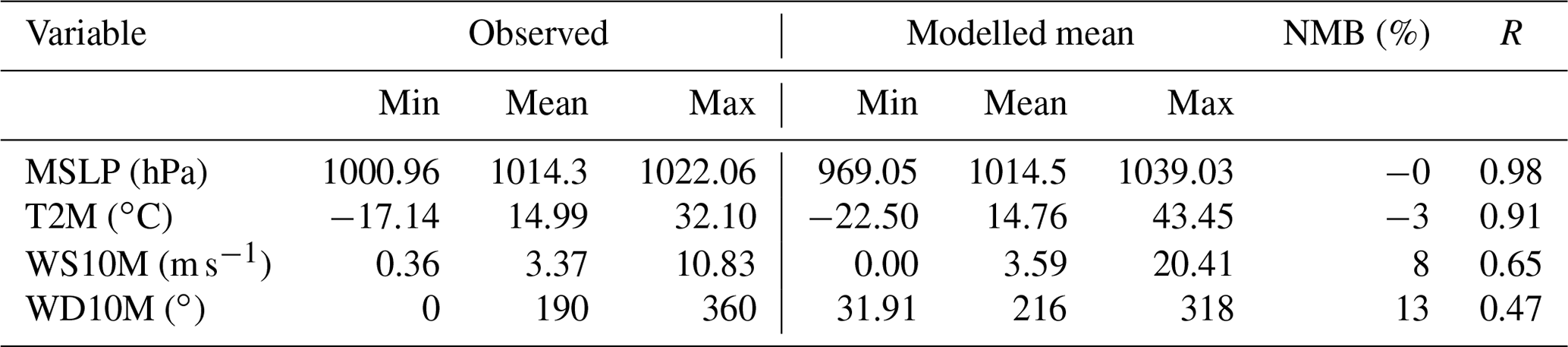
Since the accurate simulation of meteorological parameters represents a key factor affecting the concentrations of trace gases, we briefly compare the modelled mean sea level pressure (MSLP), 2 m temperature (T2M), and 10 m wind speed (WS10M) and direction (WD10M) variables against GWO measurement. Predicted model variables were then evaluated against observations using statistical scores that include normalised mean bias (NMB) and the correlation factor between simulated and measured values (r).

An extensive evaluation of WRF-Chem using the MOZART chemical mechanism to predict long-term meteorological data and O₃ levels has been presented previously (Mar et al., 2016). The main differences between the set-up used in this study and the model described by Mar et al. (2016) include differences between the versions of the model used (3.7.1 vs. 3.5.1, respectively), horizontal resolutions (50 km×50 km vs. 45 km×45 km, respectively), microphysics (Morrison vs. Lin, respectively) and cumulus schemes (Grell–Freitas vs. Grell 3-D, respectively), simulation years (2010 vs. 2007, respectively), anthropogenic emissions inventory (TNO-MACC III vs. TNO-MACC II, respectively), and chemical input and boundary conditions (extended CAM-Chem version 1.2 with MOZART-4 vs. MOZART-4/GEOS-5 simulations found at https://www.acom.ucar.edu/wrf-chem/mozart.shtml, last access: 15 June 2018, respectively).

Due to the coarse resolution of our domain, the air parcel dynamics associated with the complex topography of mountainous areas was not properly reproduced. Thus, we assessed the ability of the model to reproduce the meteorological variables using only those sites located below 1500 m above sea level. MSLP data were well reproduced over the entire period (NMB =0 % and r=0.98). The model predicted T2M values well (r=0.91); however temperature was underestimated by 3 % (see Table 2). WS10M was also fairly well reproduced in terms of both spatial and temporal variability (NMB =8 %, r=0.63). Yet, WD10M data could not be predicted as well as other meteorological variables (NMB =13 %, r=0.47); behaviour could be related to the existence of unresolved topography features (Jiménez and Dudhia, 2012). However, the model performance is similar to Mar et al. (2016) and Tuccella et al. (2012).

Table 2 Observed mean and simulation summary statistics for meteorological parameters. The normalised mean bias (NMB) and correlation coefficient (R) are calculated between simulated and observed meteorological observation from GWO during the April–September 2010 period.

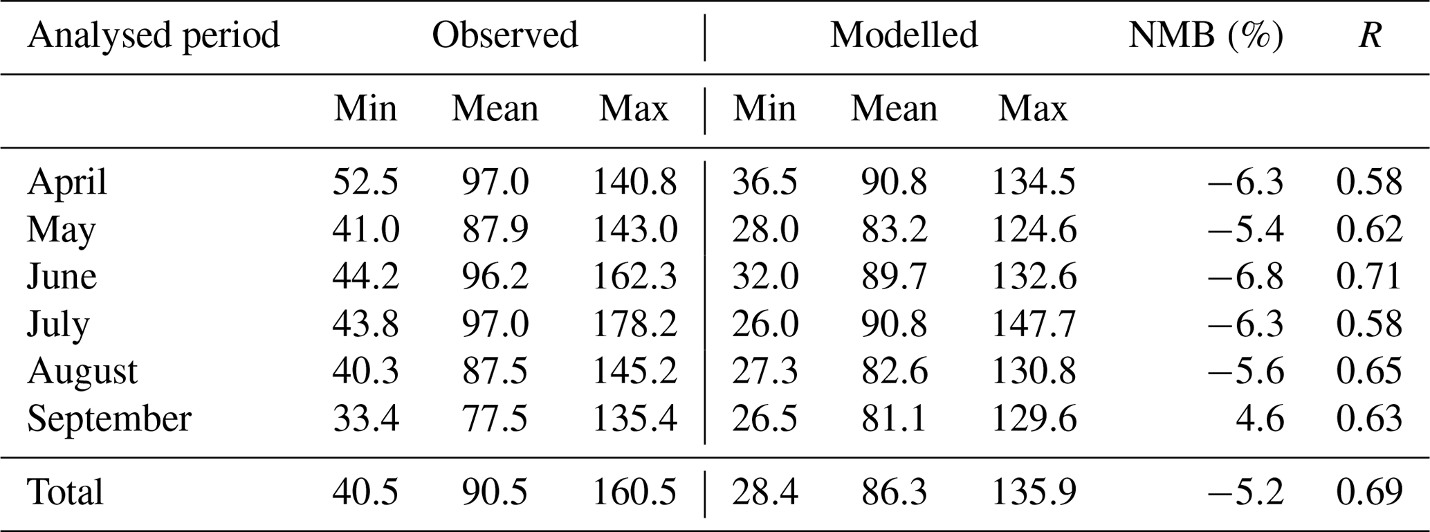
We also compared modelled MDA8 O₃ concentrations with observations provided by the publicly available AirBase dataset. The relatively coarse resolution of the domain may not be representative of changes in local emissions when the measurements are taken from urban areas; therefore, to aid in the analysis, we used only those stations characterised as rural. As can be seen in Table 3, evaluation of the model over the entire period revealed that the model performs quite well with respect to the prediction of concentration and temporal evolution. Mar et al. (2016) reported a mean bias (MB) value of 15.85 µg m⁻³ and an NMB of 17 % for the June–August 2007 period when the MOZART mechanism was used to assess the chemical performances of the model. For the same time period, we obtained an MB value of −5.92 µg m⁻³ and an NMB value of −6.3 %. Tuccella et al. (2012) reported an annual MB of −1.4 µg m⁻³ when the RADM2 chemical mechanism was used to simulate a period throughout 2007. Month-to-month analysis (Table 3) shows that the model reproduces the O₃ concentration well compared to Mar et al. (2016) and Tuccella et al. (2012). Even though the performance of the model in terms of temporal variation is relatively good (r values fall between 0.58 and 0.71), it mostly underestimated concentrations of O₃, except in September, when the model overestimated concentrations (NMB =4.6 %). Errors of the model may be explained by a wide range of uncertainties related to modelled physical and chemical processes such as grid resolution, vertical and horizontal transport, boundary-layer mixing, emission inventory, chemistry and photolysis rates, dry deposition, wet scavenging, etc. It is also possible that uncertainties in measurements contribute to observed errors. Since the focus of this study is on the contribution of different sources of precursors to the total tropospheric O₃ concentration of a particular area, a more thorough analysis of the ability of the model to reproduce the observed meteorological variables is beyond the scope of this paper.

Table 3 Observed mean and simulation summary statistics for MDA8 O₃ concentrations (µg m⁻³) at rural background sites. The normalised mean bias (NMB) and correlation coefficient (R) are calculated between simulated and observed O₃ concentrations from the AirBase dataset during the April–September 2010 period.

3.2 Contribution of tagged precursor sources to the MDA8 O₃ mixing ratios

Figure 2 shows the spatial distributions of simulated monthly mean MDA8 values from tagged O₃ source regions and other global source types throughout late spring in 2010. The receptor regions shown were mainly influenced by the overseas combination of NAM, ASI, OCN, and RST sources that combined contribute from 23 % in the Po Valley to up to 53.6 % in the UKI region (see Table S1 in the Supplement). O₃ from RST (a 7.5 %–15 % contribution) is the main source from overseas. O₃ from shipping NO_x emissions advected through the model boundaries combined with O₃ produced from shipping NO_x emissions in the Atlantic Ocean mostly affects Atlantic coastal countries (up to a 16.1 % contribution in the UKI region), yet a small contribution of ∼4 %–5 % was also observed within inland regions. Long-range transport of O₃ from Asia and North America contributes significantly to total observed O₃ in Europe, accounting for 9.6 % of the total observed O₃ in ITA and up to ∼22 % in UKI and SCA. After intercontinental transport, O₃ produced within Europe is an important source of O₃ in receptor regions, followed by O₃ coming from other global source types (LGT, BIO, and BMB). In general, for the April–May 2010 period, the contribution from the local sources to the total MDA8 O₃ mixing ratio in receptor regions falls within a range from 8.5 % (SCA) to 21 % (RBU) (see Table S1). Emissions from local sources do not only affect local O₃ mixing ratios, but also impact O₃ levels of bordering countries due to strong horizontal pollution transport. In all receptor regions, local anthropogenic sources have a lower contribution to MDA8 O₃ mixing ratios than the sum of O₃ due to anthropogenic sources in other European source regions and long-range transport of ozone from intercontinental source regions. The contribution of intercontinental transport to the total MDA8 O₃ mixing ratio in Europe is consistent with previously reported results, i.e. Fiore et al. (2009) and Karamchandani et al. (2017), while this study allows us to identify which anthropogenic sources exert a strong influence on MDA8 O₃ predicted in different regions. Using observations, Danielsen (1968) and Thouret et al. (2006) showed that the transport of O₃ from the stratosphere also contributes to tropospheric O₃. Here, stratospheric O₃ contributes up to 7 ppb (12.5 % in SCA) to the total MDA8 O₃ mixing ratio, which is a finding similar to that reported by Derwent et al. (2015). A similar tagged system for predicting O₃ levels, using the CAM-Chem model (Butler et al., 2018), has also shown that stratospheric O₃ significantly contributes to the total tropospheric O₃ mixing ratio. The MOZART chemical mechanism used in this study does not explicitly treat stratospheric chemistry; thus surface stratospheric O₃ could be attributed to the vertical and horizontal transport of stratospheric O₃ and stratospheric tagged precursor species concentrations coming from the CAM-Chem extended model that enters the domain through lateral boundaries.

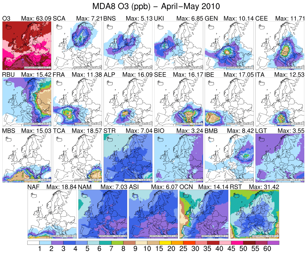
Figure 2 Contribution to MDA8 O₃ (ppb) of each O₃ source region and global source type for the April–May 2010 period.

During June–August 2010, western Europe was mostly influenced by a high-pressure system centred over the Atlantic (see Fig. S1 in the Supplement). In the upper troposphere, a ridge influenced the vertical atmospheric structure, especially over southern Europe. Therefore, these “usual summer conditions” favoured the intrusion of warm air coming from Africa and the Arabian peninsula and led to a warm and dry climate characterised by subsidence, stability, clear skies, and high-intensity solar radiation. Hence, the photochemical formation of O₃ was enhanced and influenced the stronger contribution of local emissions to the total mixing ratio compared to the previous period examined. Figure 3 depicts the average MDA8 O₃ for June–August 2010. For most regions, we notice that levels of O₃ produced from local sources from June to August compared with April–May were enhanced (Fig. 2). Local sources can contribute to more than 20 % of the mean MDA8 O₃ mixing ratio (from 14.6 % in SCA to 35.7 % in the Po Valley; see Table S1). This shows that local sources play a strong role in the formation of O₃ throughout the June–August period, as has been previously shown by Jiménez et al. (2006) and Querol et al. (2018). Compared with late spring, the relative contribution of overseas sources decreased in summer, varying from 10.9 % in the Po Valley receptor region to 44.8 % in the UKI region in the month of July (Figs. 2 and 3; Table S1). We noticed the spread of O₃ produced from European anthropogenic precursors over bordering regions compared with late spring 2010 (Figs. 2 and 3). The increase in average temperature combined with stable atmospheric conditions led to an enhancement of the biogenic NO emitted into the atmosphere, especially in southeastern and eastern Europe; thus, the BIO global source type contributes up to ∼9 ppb (13.2 % of MDA8 O₃) in the RBU receptor region (see Fig. 3). The vegetation fires that took place across Russia in July and August (Gilbert, 2010; Huijnen et al., 2012) as well as in Portugal and Spain (European Commission, 2011) lead to increases in the contribution of O₃ coming from BMB of up to 29 ppb (16 %) in the RBU receptor region and up to 8.5 ppb (2.3 %) in the IBE receptor region. BMB emissions contribute domain-wide more than 3 % (Po Valley), with the greatest impacts modelled over RBU, IBE, SEE, SCA, and TCA. The enhanced photochemical activity during summer combined with the weakening of stratospheric–tropospheric exchange reduce the influence of stratospheric O₃ from a domain-wide mean MDA8 O₃ mixing ratio of 4.4 ppb in the spring to 1.3 ppb in the summer (Figs. 2 and 3).

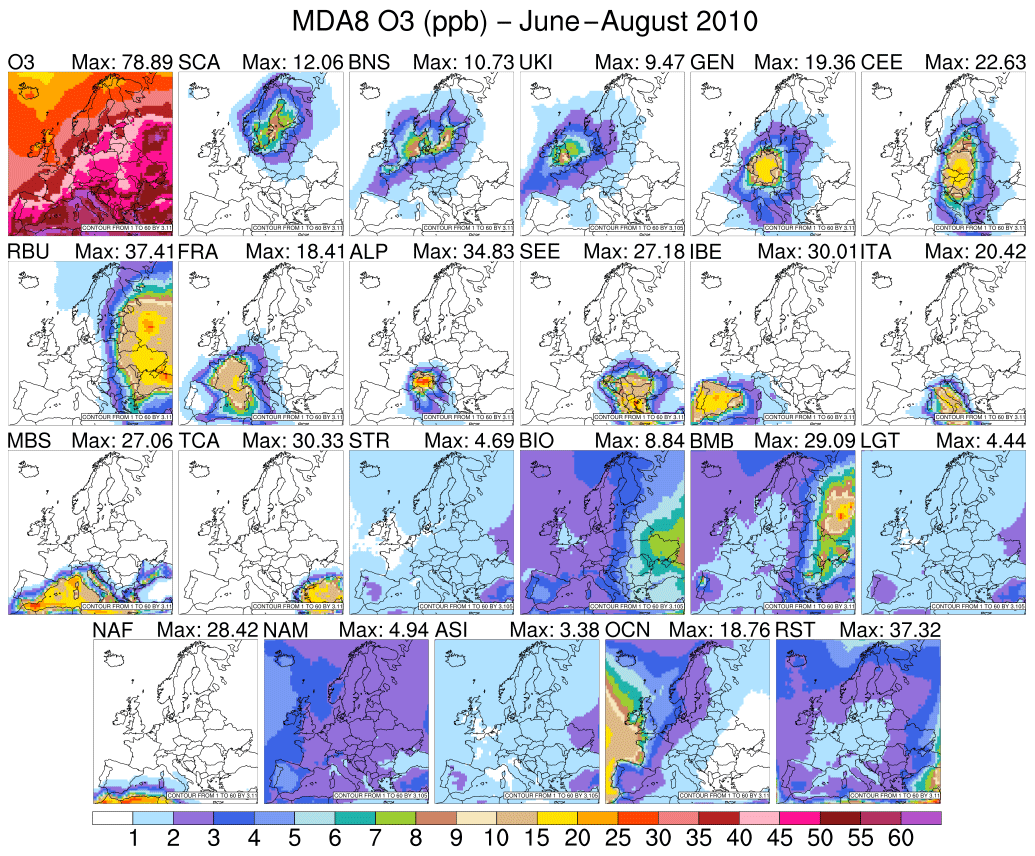
Figure 3 Same as Fig. 2, but for the June–August 2010 period.

The decrease in photochemical activity in September 2010 is reflected in decreases in total O₃ mixing ratios compared with the summer of the same year as well as in a reduction associated with the local source contribution to the total O₃ mixing ratio (Fig. 4). Thus, only in IBE, TCA, FRA, Po Valley, the high Alps, and RBU regions was contribution of local sources to total MDA8 O₃ higher than 20 % (Table S1). On the other hand, we noticed an increase in O₃ coming from anthropogenic overseas sources and from lightning in autumn, stressing that seasonal variations exist within the outflow from other continents. There is also variation in the lifetime of O₃, which is shortest during the summer as a result of enhanced photolytic activity.

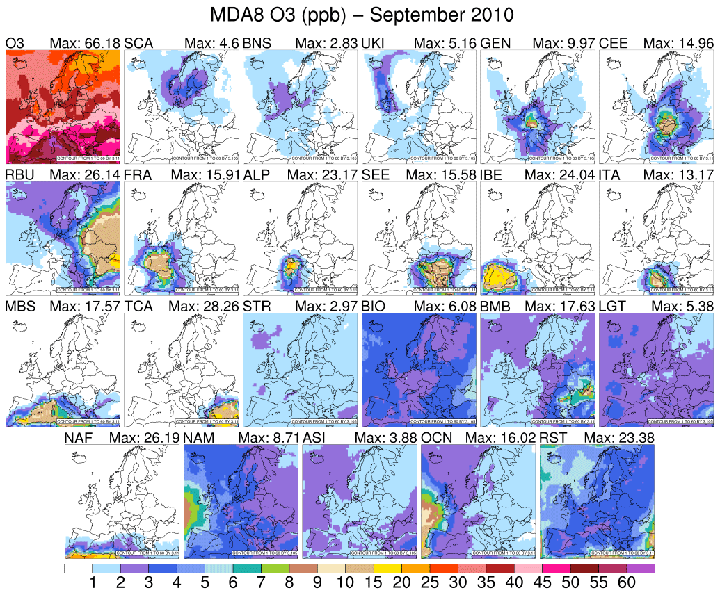
Figure 4 Same as Fig. 2, but for September 2010.

Although we have seen that long-range transport plays a major role in total O₃ mixing ratios, the tagging technique helps to gain more insight into which region of the world dominates these mixing ratios in spring or autumn. In early autumn, the western European receptor regions exhibit a slight increase of 1.6 % in O₃ mixing ratios coming from North America compared with spring, while the contribution of O₃ mixing ratios coming from other overseas sources decreases. This could be linked to the prevailing westerly wind and the synoptic conditions seen during the first period of September, when the Azores High extended far to the east and north (Fig. S1). This phenomenon creates conditions that are conducive to the transatlantic transport of American pollution in the eastern direction. For example, in autumn periods within the RBU receptor region, North American and oceanic sources account for up to 14.6 % in spring and 11.4 % in autumn of the MDA8 O₃ mixing ratios.

Apart from local and other global source types, NO_x emissions from shipping activities in the Atlantic Ocean combined with the oceanic O₃ from boundary conditions are an important source of O₃ that explains up to 16 % in late spring, 21 % in summer, and 12 % in early autumn of the MDA8 O₃ mixing ratio in the UKI, IBE, FRA, GEN, CEE, and SCA regions. Butler et al. (2018) showed that O₃ from oceanic sources reaches a minimum level in the North Atlantic Ocean during the summer, yet this study shows that in the UKI, IBE, FRA, GEN, CEE, and SCA receptor regions the oceanic O₃ contribution peaks in the summer. This implies that the nearby shipping emissions have a greater impact on oceanic bordering countries rather than oceanic O₃ from boundary conditions. Furthermore, the NO_x emissions from shipping activities in the Mediterranean and Black seas account for up to 14 % in late spring, 19 % in summer, and 11 % in early autumn of the MDA8 O₃ mixing ratio predicted in the receptor regions situated along the shore of the Mediterranean Sea, such as IBE, ITA, SEE, and FRA.

Our model results have shown that the highest MDA8 O₃ mixing ratios are predicted to occur over the Mediterranean Basin. This is due to the presence of favourable conditions for O₃ formation including the presence of small deposition sinks and intense photochemistry (Figs. 2–4). Several studies, such as Safieddine et al. (2014), Tagaris et al. (2017), Mertens et al. (2018), Querol et al. (2018) and the references therein, have used source attribution methods to establish the origin of tropospheric O₃ observed over the Mediterranean Basin. The tagging technique used here shows that the O₃ from shipping activities in the Mediterranean and Black seas (MBS) explains, on average, 15 % in late spring, 20 % in summer, and 12 % in early autumn of total MDA8 O₃ predicted to accumulate within the MBS receptor region. These findings are similar to those of Aksoyoglu et al. (2016) that showed these emissions accounted for 10 %–20 % of the mean O₃ in the Mediterranean in the summer of 2006. Moreover, Tagaris et al. (2017) have shown that shipping emissions explain up to 30 % of the MDA8 O₃ simulated for July 2006 over the Mediterranean Sea. This study has shown that the shipping activities likely accounted for up to 35 % of the MDA8 O₃ near the Strait of Gibraltar (see Fig. 5) during the April–September 2010 period. Shipping emissions contribute most highly to total O₃ in the western basin of the Mediterranean Sea. Aside from shipping activities, the other European source regions have a localised contribution to total MDA8 O₃ predicted in the Mediterranean Sea. Thus, ITA, ALP, and GEN source regions contribute mostly to the central basin; IBE and FRA are the main contributors in the western basin and SEE and TCA predominantly contribute to the eastern basin. Natural sources contribute on average up to 10 % of MDA8 O₃ in the western basin and up to approximately 25 % of MDA8 O₃ in the eastern basin. The long range of O₃ transport contributes up to 45 % along the north African shore and it exhibits a zonal pattern, with low mixing ratios occurring in the north and high mixing ratios occurring south of the Mediterranean Sea, a trend mostly due to O₃ mixing ratios from NAF and RST sources.

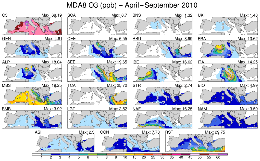
Figure 5 Average MDA8 O₃ mixing ratio (upper left panel) and contribution of each tagged O₃ source region and global source type over the Mediterranean Sea for the April–September 2010 period. The unit is parts per billion.

3.3 Tagged ozone precursor contributions to exceedances of MDA8 target values – case study

As previously mentioned, the European Air Quality Directive (EU directive 2008/50/EC, 2008) has defined a target value of 120 µg m⁻³ for the MDA8 O₃ concentration, which can be exceeded up to 25 d per calendar year (over a 3-year span). In the following, we refer to values that surpass 120 µg m⁻³ as exceedances and values below 120 µg m⁻³ as non-exceedances. Figure S2 shows the spatial distribution of the number of exceedances observed and calculated throughout the April–September 2010 period for the AirBase rural stations. The observed MDA8 O₃ exceeds the target limits locally in Po Valley, Austria, and Germany; in coastal areas of Portugal, Spain, France, and Italy; and inland areas of Poland and Slovakia. However, the modelled exceedances do not exhibit the same spatial pattern or intensity as observed values. Our use of tags allows for the identification of main source contributors to exceedances of modelled MDA8 O₃. Given the high number of stations that measure O₃, for simplicity, we will discuss the source contribution to the MDA8 O₃ exceedances only for the Po Valley, high Alps, and GEN receptor regions.

Figure 6 exhibits the contribution of each tagged source and type to modelled and to observed MDA8 O₃ values. Samples were, in all cases, taken at the location of the measurement stations, throughout the April–September 2010 period. Figure 6 shows the average conditions during the exceedance of the MDA8 O₃ target value, and also, at times, occurred when the target value was not exceeded. To perform the source attribution for the observed values, we have scaled these values proportionally by the relative concentrations of each tagged O₃ tracer in our model output.

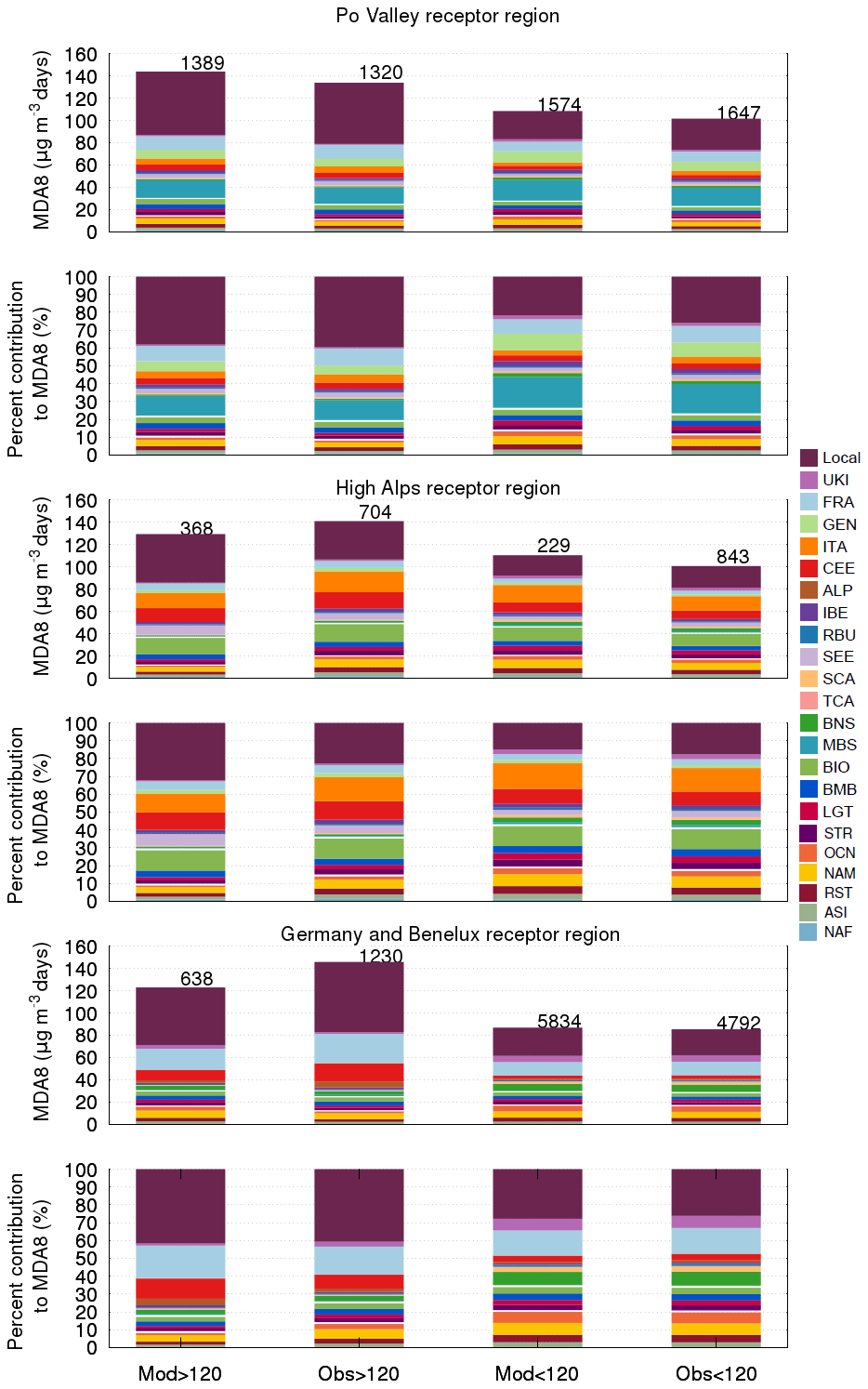
Figure 6 Mean modelled and observed MDA8 O₃ mixing ratio filtered by a threshold of 120 µg m⁻³ for the Po Valley, (top panel) high Alps (third panel from top), and GEN (fifth panel from top) and percent contribution to MDA8 O₃ from different emissions sources and types for the Po Valley (second panel), high Alps (fourth panel) and GEN (bottom panel) during the April–September 2010 period. In each case the contributions of tagged sources to the total O₃ are shown. The tagged contributions of local and other European sources, HTAP2 source regions, and other global source types to observed O₃ are obtained by scaling the observed O₃ by the relative contributions of these tagged sources to modelled O₃. The total number of exceedances (and non-exceedances) of the MDA8 O₃ target value is indicated at the top of each column.

The relative contribution of emissions from different source regions to modelled and to observed MDA8 O₃ values, after being scaled to account for the contribution of modelled sources of O₃ types, is generally similar for the Po Valley and GEN receptor regions (see Fig. 6). In the Po Valley, we can pinpoint the main remote contributor as being MBS (see Fig. 6), followed by GEN and FRA, suggesting a dominant westerly and northerly air flow. The recirculation of air masses in the Gulf of Genoa could accentuate the sea breeze, and therefore more O₃ coming from NO_x associated with shipping activities in the Mediterranean will be transported to the coastal and inland stations.

The high Alps receptor region is less influenced by ALP emissions than the Po Valley, and it is more influenced by remote sources (see Fig. 6). The increased contribution of O₃ from CEE, ITA, and FRA to both exceedance and non-exceedance days in the high Alps receptor region compared with the Po Valley receptor region highlights the impact of the transboundary transport of O₃ and its precursors. Furthermore, the contribution of stratospheric as well as long-range sources was generally 6 % higher in this receptor region than in the Po Valley receptor region.

In GEN, the main remote source regions are FRA and CEE during the exceedance days and FRA and UKI during non-exceedance days (Fig. 6). Opposite to the Po Valley, in GEN the model predicts fewer MDA8 O₃ exceedance days. Comparing the source contribution to both modelled and observed exceedance days, we noticed that the model underestimates O₃ concentrations associated with long-range transport and natural sources. Further, the model predicted higher levels of O₃ from CEE and FRA than observed. Underestimation of long-range-transported O₃ into the GEN region in our model could be explained by the fact that the number of modelled MDA8 O₃ exceedances in GEN is half of the observed number of exceedances (Fig. 6).

This kind of analysis can be applied to improve our knowledge of the origin of O₃ precursors and their contribution to MDA8 O₃ health metrics. Hence, by using this tagging technique, policymakers can identify future actions required to control the NO_x emissions at local and regional levels.

3.4 Tagged ozone precursor contributions to regulatory ozone metrics

In this section, we discuss the contribution of O₃ mixing ratios from diverse emissions sources and types to several metrics that quantify the O₃ exposures of humans and ecosystems. From modelled hourly mixing ratios of tagged O₃ sources and other global types, we have calculated different O₃ metrics, including non-cumulative (mean, MDA8, and the 95th percentile O₃) and cumulative (SOMO35, W126, and AOT40) metrics. We have chosen not to analyse the performance of the calculated cumulative metrics in comparison with measured values, as was done in previous work by Tong et al. (2009). Their work showed that the poor performance of the cumulative metrics is closely related to the sensitivity of these metrics to the threshold values or weighting factors.

Figure 7 and Table S2 include the percentage of the contribution of different sources of emissions and other global types to total O₃ as calculated using health and vegetation metrics. The non-cumulative O₃ metrics employed in this study have displayed similar patterns for most of the receptor regions. The contribution of local and European sources to the total O₃ mixing ratios has been low when we applied to mean O₃ metric and high when using the 95th percentile metric. These findings emphasise the importance of O₃ produced by local and neighbouring sources to the high end of the O₃ mixing ratio distribution.

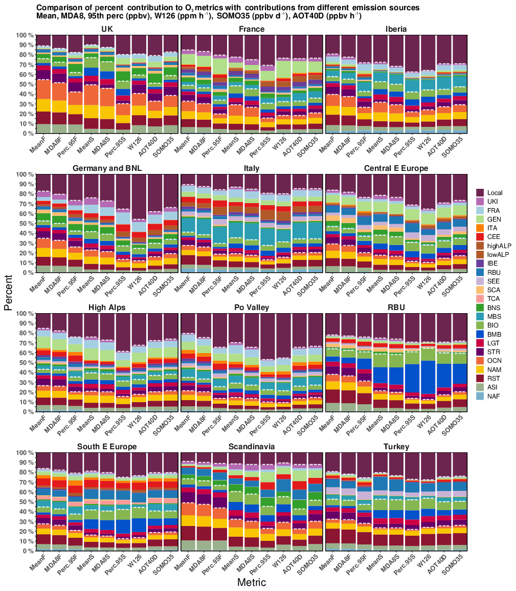
Figure 7 Comparison of percent contribution of local and other European sources, HTAP2 source regions, and other global source types to different O₃ metrics. The metrics analysed are mean, MDA8, and 95th percentile (ppb) for the early “F” and late “S” simulation periods, W126 (ppm ⋅ h), SOMO35, and AOT40 (ppb ⋅ h). The white dashed lines in each panel separate different categories (intercontinental transport, other global source types, and local and other European sources).

Splitting the non-cumulative metrics into early (April–June) and late (July–September) simulation periods clearly illustrates that the European receptor regions are more prone to be influenced by intercontinental transport during the early period than the late period. The contribution of inter-continentally transported O₃ to mean O₃ values in different receptor regions is higher during the early period and it spans between 22.8 % and 54.3 % of total O₃. In the late period it accounts for between 16 % and 48.9 % of total O₃ (see Fig. 7 and Table S2). Since O₃ associated with intercontinental transport comes, in this case, solely from boundary conditions, errors in boundary conditions affect the predicted mixing ratio of various chemical species and, consequently, the contribution of overseas sources of O₃ to levels observed in Europe O₃ (Tang et al., 2007; Giordano et al., 2015; Im et al., 2018).

The shorter lifespan of O₃ over remote ocean regions throughout the warm season, combined with synoptic conditions, has led to decreased levels of inter-continentally transported O₃ to Europe. Thus, for most receptor regions, the O₃ coming from Asia and the rest of the world was reduced by more than half when compared with the cold period. The O₃ mixing ratio from the stratosphere is, in general, 2.5 times higher in the cold season than in the warm season, which is consistent with the findings of a study by Butler et al. (2018), which showed that the stratospheric O₃ mixing ratio varies with altitude and its lifetime is influenced by season and latitude. The tagging technique also helps to quantify the impact of biogenic and biomass burning emissions of NO_x on tropospheric O₃. The impact of biogenic NO_x emissions on mean O₃ mixing ratios is between 3.3 % in the Po Valley and 5.9 % in TCA in the early season, while during the late season it is between 5.4 % in the Po Valley and 13.4 % in RBU. The biomass burning emissions account for variable percentages of mean O₃ mixing ratios. These span between 1.6 % in ITA and 5.3 % in RBU during the early season and between 3.8 % in the Po Valley and 16.3 % in RBU during the late season. Natural sources do not usually vary greatly when different non-cumulative metrics are applied. An exception would be for the biomass burning emissions in RBU during the late season. Thus, BMB in RBU contributes to 16.3 %, 17.6 %, and 28.8 % of the mean, MDA8, and 95th percentile, respectively.

Even though the SOMO35 and AOT40 metrics are not accumulated over the same period (SOMO35 is accumulated over the entire simulated period, and the AOT40 metric is accumulated over the May–July period) and do not use same input data (daily MDA8 O₃ for SOMO35 vs. daytime O₃ mixing ratios for AOT40), since they are based on threshold exceedances and are designed to measure exposure to high O₃ levels of humans (SOMO35) and vegetation (AOT40), there is a way to directly compare data from each metric type. As shown in Fig. 7 and Table S2, the contribution of different sources of emissions and types as a proportion of total SOMO35 and AOT40 metrics is similar for most of the European receptor regions. Their spatial distribution (not shown) is also comparable, with minimum values over the UK, NW Europe, and Scandinavia and maximum values over Italy, the Alps, south of Spain, east of Turkey, and in the metropolitan area of Moscow, Russia. These results are consistent with previous studies performed by Aksoyoglu et al. (2014) and Anav et al. (2016). The overseas sources contribute similarly to SOMO35 and AOT40 indexes (usually less than 30 %) for most of the receptor regions used in this study. However, in UKI the overseas sources account for 32 % of AOT40 and 38 % of SOMO35, and in SCA they contribute to ∼22 % of AOT40 and 30 % of SOMO35. This suggests that these metrics are more sensitive with respect to the O₃ mixing ratios from remote sources in areas having a low level of O₃ pollution. In the RBU receptor region, these indicators are sensitive to O₃ coming from biomass burning emissions (20 % of SOMO35 and 24 % of AOT40), whereas for the remaining receptor regions the contribution of natural sources to SOMO35 and AOT40 is similar. Local sources account for a range of ∼12 % (SCA) to ∼38 % (GEN) of these metrics. These data highlight the occurrence of increased O₃ production from local sources in comparison with northern European countries as well as large emissions of NO_x in the GEN source region. Since the difference between AOT40 and SOMO35 is only a few percentage points, regardless of the receptor region, we were able to conclude that they behave similarly, according to thresholds used to define these metrics.

The tagging method allows a better understanding of the main precursor sources responsible for exceedances of regulatory O₃ metrics. This information can help to inform further modelling studies aimed at investigating the effects of emission reduction strategies and ultimately inform air quality policy. For example, in the Po Valley receptor region, the modelled AOT40 is up to 3.4 times higher than the target limit given by EU legislation (on average 31 218 ppb ⋅ h). The observed and calculated AOT40 values depicted in Fig. S3 exhibit the exceedance of target limits in the Po Valley. O₃ coming from local sources can explain 35.0 % of this value (an average of 10 909 ppb ⋅ h). After local sources, the main European anthropogenic sources contributing to high AOT40 values in the Po Valley region are from FRA (6.6 %), GEN (7 %), and MBS (8.8 %) (Table S2). Generally, the O₃ mixing ratio and its precursors transported from other anthropogenic European sources into the Po Valley receptor regions account for ∼39.5 %, while natural sources account for ∼12.3 % and long-range transport accounts for ∼13.4 % of the remaining AOT40 mixing ratios. Thus, to reach at least the target limit in the Po Valley receptor region, considerable emission reductions will still be needed, not only on a local scale but also on the European scale, especially within the MBS, GEN, and FRA source regions.

Figure 7 also shows the percentage that different types of emissions and emission regions contribute to the W126 index. Interestingly, for most of the receptor regions, local NO_x anthropogenic emissions cause the largest response in W126 values compared with the other cumulative metrics used in this study. Thus, local NO_x explains from 10.9 % (0.1 ppm ⋅ h) in SCA to more than 40 % of W126 in GEN (45.9 %; 2.48 ppm ⋅ h) and the Po Valley (45.4 %; 8.7 ppm ⋅ h) of W126 index values calculated for each region. The effect of European transported plumes is also enhanced when using the W126 index compared with the other metrics for most of the downwind receptor regions. This behaviour is related to how these metrics have been defined. Due to its sigmoidal weighted formulation, as discussed in Westenbarger and Frisvold (1995) and Lapina et al. (2014), W126 includes all daytime values rather than O₃ levels above a certain threshold, as is done using SOMO35 and AOT40; therefore lower weighting factors of less than 0.5 are given to low O₃ values and weighting factors above 0.5 are given to O₃ values situated above the inflection point of 67 ppb.

The modelled mean AOT40 and W126 values in the Po Valley receptor region exceeded standards (26 368 ppb ⋅ h for AOT40 and 28.9 ppm ⋅ h for W126) during the May–July 2010 period, and, as shown in Fig. 7 and Table S2, local sources are an important contributor to these metrics. To better understand why the W126 index is mainly influenced by local sources compared with the other cumulative metrics, we thoroughly compared AOT40 and W126 values for the Po Valley receptor region. As shown in Fig. 8, a temporal series of hourly daylight values for mean O₃, W126, and AOT40 values averaged over the Po Valley receptor region are given. Since the W126 unit is ppm ⋅ h, a more direct comparison with the W126 index would require values to be expressed in ppb ⋅ h. Further, all metrics showed a similar level of temporal variation in which they peaked in the first half of July. Also, whenever the averaged O₃ mixing ratio was lower than 60 ppb (Fig. 8a), the W126 value was lower than AOT40 (Fig. 8d). This way of acting was most probably due to the weighting factor being less than 0.3, and above this mixing ratio W126 tends to be higher than AOT40. This behaviour is closely linked to the definition of these metrics. If the O₃ mixing ratio is less than 40 ppb, W126 has a weighting factor lower than 0.03, while AOT40 has a weighting factor of 0. Above this threshold, AOT40 has a weighting factor of 1, while in the case of W126 only O₃ values higher than 100 ppb have a weighting factor of 1. Due to the way these metrics are defined, predicted O₃ values in each grid cell are taken into account for the W126 but may not be taken into account for the AOT40 index.

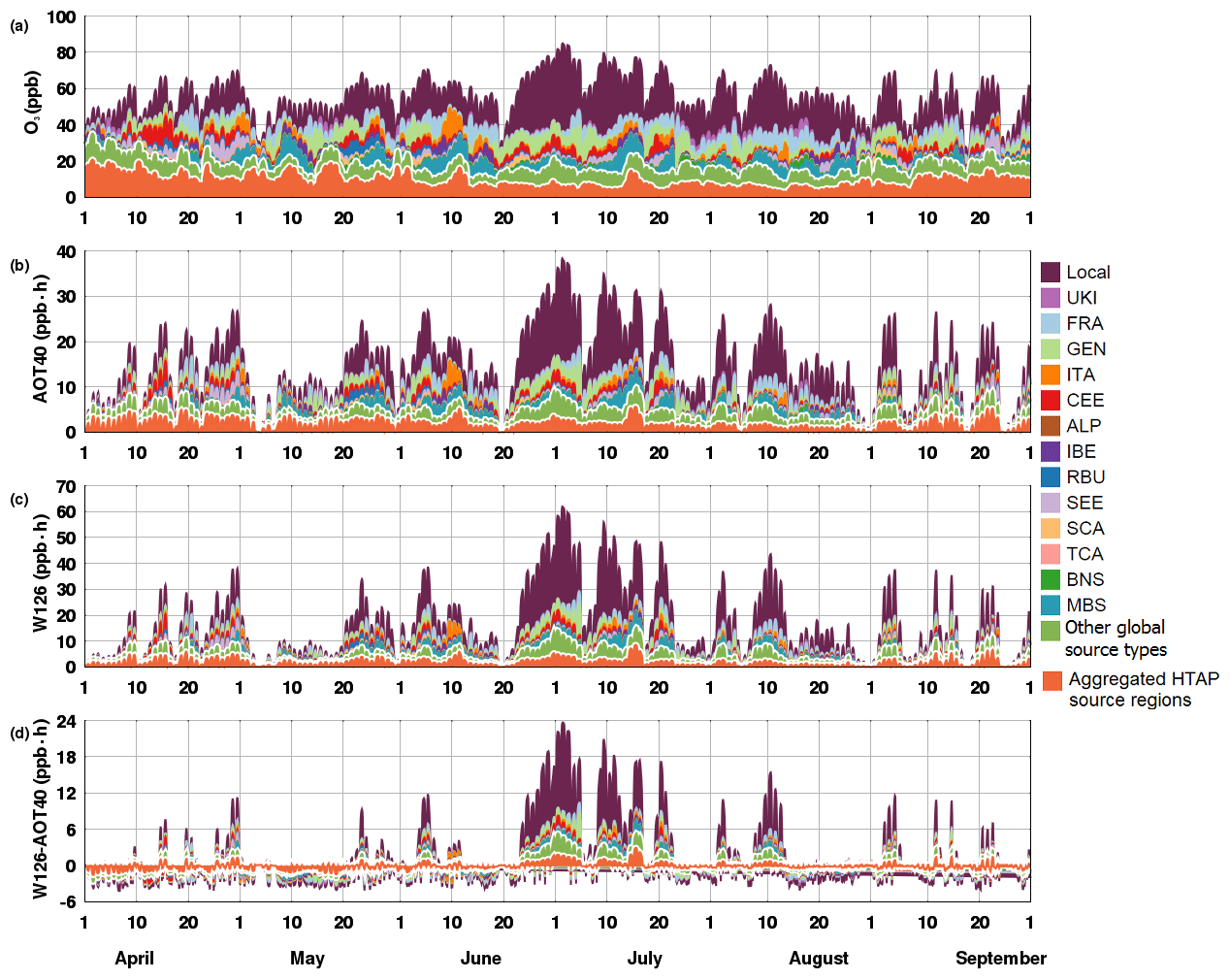
Figure 8 April–September 2010 time series of daytime (a) hourly O₃ (ppb), (b) hourly AOT40 index (ppb ⋅ h), (c) hourly W126 index (ppb ⋅ h), and (d) differences between W126 and AOT40 indexes (ppb ⋅ h) averaged over the Po Valley receptor region. The colour bars indicate the O₃ source categories – aggregated HTAP2 regions (ASI, NAM, NAF, OCN, and RST), the other global source types (STR, LGT, BMB, and BIO), and the European source regions. The white dashed lines in each panel separate different categories (intercontinental transport, other global source types, and local and other European sources).

In addition, visual analysis of the time series also revealed that when the O₃ mixing ratios from local sources are ∼20 ppb, these mixing ratios have a higher contribution to W126 than AOT40. To better understand this observation, we have further analysed the relationship between mean O₃ values from ALP sources (O₃-ALP) and the percent contribution of these O₃ tracers to mean O₃, W126, and AOT40 metrics. Figure 9 shows scatter plots for O₃-ALP that relate the contributions of these mixing ratios to mean O₃, W126, and AOT40. In addition, the linear regressions of Y vs. X ($Y=a\cdot X+b$) using all datasets have been applied. We saw that in general, high mean O₃-ALP mixing ratios have a higher contribution to W126 than to AOT40; this was also confirmed by the linear regression between O₃-ALP and W126 that yields a slope of 1.52 compared to a slope of 1.36 obtained when the linear regression was applied to AOT40 vs. O₃-ALP. Averaged O₃-ALP and mean O₃ as well as O₃-ALP and W126 were highly correlated (r=0.96 and r=0.93, respectively), while O₃-ALP and AOT40 are correlated more loosely (0.88). The high level of correlation between O₃-ALP and both mean O₃ and W126 could be related to the fact that these metrics account for all modelled values, whilst AOT40 considers only O₃ values above 40 ppb.

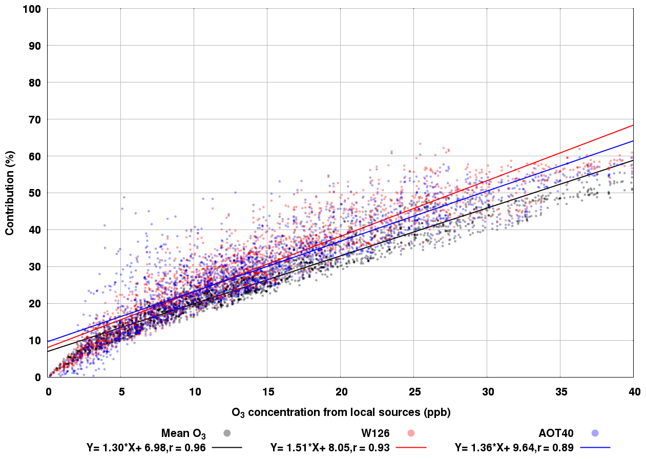
Figure 9 Scatter plots showing the ozone concentration from local sources versus the contribution to mean O₃ (black dots), W126 (red dots), and AOT40 (blue dots). The solid lines are the lines of best fit.

Extending this analysis to all receptor regions, we can explain why the W126 index is more sensitive to O₃ coming from local sources compared with the other cumulative metrics. In addition, W126 accentuates the contribution of BIO and BMB in RBU, TCA, and SEE, most likely because the metric includes all daytime values and not just those above a certain threshold. Thus, the use of W126 highlights the considerable impacts of BIO and BMB emissions on total O₃ mixing ratios throughout the summer and from burning vegetation that ultimately influence the extent to which O₃ causes damage to vegetation.

We have seen that the contribution of NO_x to total O₃ varies depending on metrics and regions considered. Hence, the tagging method could help design different emission control strategies in specific source regions depending on which impacts need to be reduced in specific receptor regions.

4 Conclusions

Here, we implemented a new chemical mechanism within the WRF-Chem model to account for source attribution of O₃ from NO_x. We investigated the origin of surface O₃ using the tagging technique from April to September 2010, as well as the contribution of different sources to O₃ metrics and their exceedance events.

Using tagged simulation from WRF-Chem, we show the spatial distribution of simulated monthly mean MDA8 from tagged O₃ source regions and other global types throughout late spring, summer, and early autumn of 2010. The contribution of different sources to O₃ production varies with season. We have identified intercontinentally transported O₃ as an important contributor to the total O₃ mixing ratio, especially in the late spring and early autumn. During summer, however, the O₃ production is dominated by national and intra-European sources. We have also identified shipping activities in the Mediterranean Sea as an important source of O₃ for the IBE, ITA, SEE, and FRA peripheral maritime receptor regions. We also analysed the main sources of MDA8 O₃ over the Mediterranean Basin and we have identified the main factors that contribute to MDA8 O₃ mixing ratios to the greatest degree. These were mainly shipping activities and the localised contribution from the bordering countries.

To better understand the origin of MDA8 O₃ exceedances, we compared modelled and observed values of MDA8 O₃ concentration in the Po Valley, high Alps, Germany, and Benelux receptor regions. Throughout days exceeding the recommended thresholds of 120 µg, the contribution from local sources was ∼41 %, 34 %, and 38 % of modelled MDA8 O₃ for the Po Valley, high Alps, and GEN, respectively. Throughout days not exceeding recommended thresholds, local emissions explain ∼27 %, 16 %, and 23 % of modelled MDA8 O₃ for the Po Valley, high Alps, and GEN, respectively. Moreover, this tagging approach revealed that the main remote sources of MDA8 O₃ are MBS, GEN, and FRA for the Po Valley receptor region and are FRA, CEE, and UKI for the Germany and Benelux receptor region. In addition, these analyses identified a persistently high contribution of transboundary sources to background O₃ concentration in the high Alps receptor region. Furthermore, by showing that the contribution of precursor sources to modelled O₃ target value exceedances in the GEN region is systematically different from the contribution of precursor sources to modelled O₃ when exceedances are observed but not modelled, we have identified a possible reason (underestimation of long-range transport) for the poor performance of our model with respect to reproducing the observed number of O₃ target value exceedances in the GEN region.

Through comparisons with different O₃ metrics, we quantified the impact of local vs. non-local NO_x on O₃ production for each European receptor region. The comparison between mean, MDA8, and 95th percentile O₃ metrics accentuates the importance of large contributions from different NO_x sources to the high end of the O₃ distribution. By analysing these metrics for two periods (April–June and July–September), we can clearly distinguish the contribution of different NO_x to total O₃ mixing ratios in each region and throughout different times of the year. When we compare the cumulative metrics, we noticed that the SOMO35 and AOT40 indexes exhibit rather similar behaviour. Considering that these metrics are not calculated over the same period nor do they use the same input data, the similar behaviour is likely due to the similar threshold values applied to define these metrics.

The use of the W126 index accentuates the importance of local emissions. To confirm this, we investigated the behaviour of modelled mean AOT40 and W126 values in the Po Valley receptor region. We noticed that when the local sources contribute to more than 20 ppb of the O₃ mixing ratios, these mixing ratios have a higher contribution to W126 than they do to AOT40, and we determined that the difference was mostly due to the definition of W126, which takes into account all O₃ values, not only those that are above a certain threshold.

Overall, this study has identified local and remote factors that contribute to the MDA8 O₃ mixing ratio during several periods as well as within different O₃ metrics. Furthermore, the method applied here could be used to design improved emission control strategies depending on which impacts need to be reduced.

Appendix A: List of chemistry modules changed to account for the new chemical mechanism

• chemics_init.F;

• module_input_chem_data.F;

• module_plumerise1.F and module_add_emiss_burn.F to account for the source attribution of biomass burning emissions to O₃ concentration;

• module_emissions_anthropogenics.F to account for the impact of anthropogenic emissions on O₃ concentration;

• module_bioemi_megan2.F and module_data_mgn2mech.F to see the impact of biogenic emissions on O₃ concentration;

• module_lightning_nox_driver.F for lightning-generated nitrogen oxides;

• Dry and wet deposition of tagged trace gases are treated by module_dep_simple.F and module_mozcart_wetscav.F; thus all tagged species have the same dry deposition velocities and wet removal rates with the corresponding non-tagged species;

• module_ftuv_driver.F to consider the photolytical reaction of the new packages;

• emissions_driver.F;

• chem_driver.F.