the Creative Commons Attribution 4.0 License.
the Creative Commons Attribution 4.0 License.
 | 29 Nov 2019
Quantifying the impact of synoptic circulation patterns on ozone variability in northern China from April to October 2013–2017
Jingda Liu
Mingge Li
Zhiheng Liao
Yang Sun
Tao Song
Wenkang Gao
Yonghong Wang
Yan Li
Dongsheng Ji
Veli-Matti Kerminen
Yuesi Wang
Markku Kulmala
The characteristics of ozone variations and the impacts of synoptic and local meteorological factors in northern China were quantitatively analyzed during the warm season from 2013 to 2017 based on multi-city in situ ozone and meteorological data as well as meteorological reanalysis. The domain-averaged maximum daily 8 h running average O3 (MDA8 O3) concentration was 122±11 µg m−3, with an increase rate of 7.88 µg m−3 yr−1, and the three most polluted months were closely related to the variations in the synoptic circulation patterns, which occurred in June (149 µg m−3), May (138 µg m−3) and July (132 µg m−3). A total of 26 weather types (merged into five weather categories) were objectively identified using the Lamb–Jenkinson method. The highly polluted weather categories included the S–W–N directions (geostrophic wind direction diverts from south to north), low-pressure-related weather types (LP) and cyclone type, which the study area controlled by a low-pressure center (C), and the corresponding domain-averaged MDA8 O3 concentrations were 122, 126 and 128 µg m−3, respectively. Based on the frequency and intensity changes of the synoptic circulation patterns, 39.2 % of the interannual increase in the domain-averaged O3 from 2013 to 2017 was attributed to synoptic changes, and the intensity of the synoptic circulation patterns was the dominant factor. Using synoptic classification and local meteorological factors, the segmented synoptic-regression approach was established to evaluate and forecast daily ozone variability on an urban scale. The results showed that this method is practical in most cities, and the dominant factors are the maximum temperature, southerly winds, relative humidity on the previous day and on the same day, and total cloud cover. Overall, 41 %–63 % of the day-to-day variability in the MDA8 O3 concentrations was due to local meteorological variations in most cities over northern China, except for two cities: QHD (Qinhuangdao) at 34 % and ZZ (Zhengzhou) at 20 %. Our quantitative exploration of the influence of both synoptic and local meteorological factors on interannual and day-to-day ozone variability will provide a scientific basis for evaluating emission reduction measures that have been implemented by the national and local governments to mitigate air pollution in northern China.
- Article
(7108 KB) - Full-text XML
-
Supplement
(3012 KB) - BibTeX
- EndNote


Tropospheric ozone (O3) is one of the air pollutants of greatest concern due to its considerable harm to human health and vegetation (Kinney, 2008; Fleming et al., 2018; Mills et al., 2018). O3 is formed through nonlinear interactions between NOx and volatile organic compounds in combination with sunlight (Monks et al., 2009, 2015). Thus, ozone levels are controlled by precursors and meteorological conditions. With industrialization advancement and rapid economic growth, northern China has become one of the most populated and polluted regions in the world. The national and local governments have implemented a series of measures to reduce emissions since 2013, and although PM2.5 has decreased significantly O3 pollution is still severe in this region (Lu et al., 2018; Li et al., 2019). Several studies have explored the variation in summer ozone in China (He et al., 2017; Liao et al., 2017; Lu et al., 2018; Li et al., 2019). However, systematic research aimed at quantifying the evolution of ozone and meteorological impacts and contributions throughout the warm season (April–October) was limited during the 5 years (2013–2017) when the Action Plan for Air Pollution Prevention and Control (http://www.gov.cn/zwgk/2013-09/12/content_2486773.htm, last access: (9 September 2019) was implemented. This lack of analysis has prevented a clear understanding of the effect of emission reduction measures on ozone in northern China from being obtained.
Meteorological factors affect ozone levels through a series of complex combinations of processes, including emissions, transport, chemical transformations and removal (Chan and Yao, 2008; Jacob and Winner, 2009; Lu et al., 2019). Meteorological conditions are the primary factor that determine the day-to-day variations in pollutant concentrations over China (He et al., 2016, 2017), whereas long-term O3 trends are influenced by both climatological (weather types, temperature, humidity, radiation, etc.) and environmental factors (changes in anthropogenic and natural sources). Therefore, the impact of reduced anthropogenic emissions on O3 variations can be estimated more accurately if we are able to quantify the meteorological influence.
Synoptic meteorological conditions have an important effect on regional ozone distribution and variation (Shen et al., 2015). A given synoptic circulation pattern represents a particular range of meteorological conditions; therefore, synoptic classification is a useful method for gaining insight into the impact of meteorology on ozone levels at a regional scale. Previous studies have demonstrated a significant connection between the weather type and surface O3 concentration; however, the relation between these two quantities varies in different regions due to differences in the topography, pollution source, local circulation, and so on (Moody et al., 1998; Cooper et al., 2001; Hegarty et al., 2007; Demuzere et al., 2009; Monks et al., 2009; T. Wang et al., 2009; Zhang et al., 2012, 2013; Pope et al., 2016; Liao et al., 2017). For example, based on the Lamb–Jenkinson weather typing technique, Demuzere et al. (2009) demonstrated increased surface O3 concentrations in summer in an easterly weather type at a rural site in Cabauw, Netherlands, whereas the opposite result was obtained by Liao et al. (2017) in the Yangtze River Delta region in eastern China. Therefore, synoptic classification and its relationship with O3 need to be explored separately in different regions. In addition, based on synoptic classification, Comrie and Yarnal (1992) and Hegarty et al. (2007) suggested a reconstructed pollutant concentration (caused by synoptic influence) algorithm, which can separate the climatological and environmental variability in environmental data. It was found that 46 % and 50 % of the interannual variability in the O3 concentration was reproduced in the northeastern United States (Hegarty et al., 2007) and Hong Kong (Zhang et al., 2013), respectively, by taking into account the interannual changes in the frequency and intensity of synoptic patterns.
At the urban scale, the daily variation in the ozone concentration is affected by both synoptic and local meteorological factors. Quantifying the contribution of local meteorological factors to day-to-day variations in ozone concentrations will provide a scientific basis and guidance for reasonable ozone reduction measures, and clarifying and quantifying the relationship between meteorological factors and ozone concentration is vital for daily forecasts of ozone pollution potential. Weather type classification prior to regression analysis is superior to a simple linear regression approach (Eder et al., 1994; Barrero et al., 2006; Demuzere et al., 2009; Demuzere and van Lipzig, 2010), and a synoptic-regression-based algorithm can reproduce the observed O3 distributions and provide a better parameterization to promote the understanding of the dependence of ozone on meteorological factors in a given urban region.
Overall, in this study, we explore how the maximum daily 8 h running average O3 (MDA8 O3) concentration varies, and we quantify the contributions of synoptic and local meteorological conditions to the ozone variability in northern China (58 cities covering Hebei, Shanxi, Shandong, and Henan provinces and Beijing and Tianjin municipalities) during April–October in 2013–2017. Our specific goals are to (1) demonstrate the characteristics and variation trends in the surface MDA8 O3 concentration; (2) classify the predominant weather types and meteorological mechanisms underlying the regional ozone levels and variability; (3) quantify the contributions of changes in synoptic circulation patterns (frequency and intensity) to the interannual variability in the O3 concentration; and (4) quantify the contributions of local meteorological factors to day-to-day variations in O3 levels and identify the prominent meteorological variables and construct an O3 potential forecast model for major cities.
2.1 Ozone and PM2.5 data
The hourly O3 and PM2.5 data during April–October 2013–2017 were derived from the National Urban Air Quality Real-time Publishing Platform (http://106.37.208.233:20035/, last access: 15 October 2019). According to technical regulation for ambient air-quality assessment (HJ 663-2013, http://www.mee.gov.cn/, last access: 15 October 2019), the MDA8 O3 concentration was calculated for each monitoring site based on the hourly data from the time period 08:00–24:00 for the days with at least 14 h of measurement data. If less than 14 h of valid data are available, the results are still valid if the MDA8 O3 concentration exceeds the national concentration limit standard. Each city has at least two monitoring sites, and the MDA8 O3 levels for a city are the corresponding averages over all sites in that city. The MDA8 O3 values were collected in only 14 cities for the time period from 2013 to 2017 and in an additional 44 cities for the time period from 2015 to 2017, and detailed information is shown in Fig. 1 and Table S1 in the Supplement. The original units for the ozone observations were micrograms per cubic meter, and the conversion coefficient from the mixing ratios (unit: ppbv) to micrograms per cubic meter was a constant (e.g., 0.5 at a temperature of 25 ∘C and pressure of 1013.25 hPa). In this study, we used the original units. Unless otherwise noted, the analysis of O3 refers to MDA8 O3 during April–October in this paper.
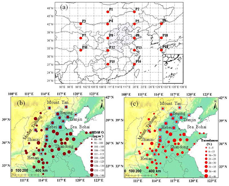
Figure 1Location of northern China (shaded area), all cities (black dots) and sea level pressure grids (a). The 16 red points show the locations of the 5∘ × 10∘ mean sea level pressure grids used for the Lamb–Jenkinson weather type classification. The spatial distributions of the maximum daily 8 h running average O3 (MDA8 O3) concentration (b) and exceedance ratios (c) for 58 cities. Statistics for 2013–2017 are shown in blue boxes; the other boxes are those for 2015–2017. The base map is topography; the elevation of the Taihang Mountains is more than 1200 m, and the Yan Mountains range from 600 to 1500 m.
2.2 Meteorological data
Gridded-mean sea level pressure data, 10 m U and V wind components (U10 and V10, respectively), boundary layer height (BLH), and 2 m temperature (T2) with a 1∘ horizontal resolution and vertical velocity (ω) from 1000 to 100 hPa (27 levels) and wind divergence (div) from 1000 to 850 hPa (seven levels) in 6 h intervals (Beijing time 02:00, 08:00, 14:00 and 20:00) for 2013–2017 were obtained from the European Centre for Medium-Range Weather Forecasts European Reanalysis Interim (ERA-Interim).
Four measurements per day for temperature (T), relative humidity (RH), total cloud cover (TCC), rain, wind speed (ws), wind direction (wd) and pressure (pre) in 58 cities during April–October 2013–2017 were obtained from the China Meteorological Information Comprehensive Analysis Process System (MICAPS). Then, daily mean meteorological factors were averaged from four measurements (scalar averaging for most factors and vector averaging for wind speed and wind direction, which involved using the u (U) and v (V) components for averaging). The meteorological station with a minimum distance from the city center was chosen.
2.3 Lamb–Jenkinson circulation typing
The Lamb–Jenkinson weather type approach (Lamb, 1972; Yarnal, 1993; Conway and Jones, 1998; Trigo and Dacamara, 2000; Mckendry et al., 2006; Demuzere et al., 2009; Russo et al., 2014; Santurtún et al., 2015; Pope et al., 2016; Liao et al., 2017) has been widely employed to classify synoptic circulation. On the basis of the Lamb–Jenkinson method, the weather type circulation pattern for a given day is described using the locations of the high- and low-pressure centers that identify the direction of the geostrophic flow; the method uses coarsely gridded pressure data on a 16-point moveable grid (Demuzere et al., 2009). In our study, northern China was set as the center. The specific schematic diagram is shown in Fig. 1a. The daily mean sea level pressure data were averaged over four time points to determine the daily weather type. The detailed classification procedure can be found in Trigo and Dacamara (2000) and in the Supplement (Sect. S1).
2.4 Reconstruction of O3 concentration based on weather types
To quantify the interannual variability captured by the variations in the surface circulation pattern, Comrie and Yarnal (1992) suggested an algorithm to separate synoptic and non-synoptic variability in environmental data; by multiplying the overall mean value of a particular pattern by the occurrence frequency of that type of year, the climate signal can be obtained as follows:
where is the reconstructed mean MDA8 O3 concentration influenced by the frequency of changes in the weather type from April to October for the year m, is the 5-year mean MDA8 O3 concentration for weather type k, and Fkm is the occurrence frequency of weather type k during April–October for year m.
Hegarty et al. (2007) suggested that variations in the circulation patterns are attributed to not only frequency changes but also intensity variations; moreover, they noted that the environmental and climate-related contributions to the interannual variations in ozone could be better separated by considering these two changes. As a result, Eq. (1) was modified into the following form:
where is the reconstructed mean MDA8 O3 concentration influenced by the frequency and intensity of the changes in circulation patterns from April to October for year m; ΔO3 km is the modified difference on the fitting line, which is obtained through a linear fitting of the annual MDA8 O3 concentration anomalies (ΔO3) to the circulation intensity index (CII) for circulation pattern k in year m. ΔO3 km represents the part of the annual observed ozone oscillation caused by the intensity in each circulation pattern. Hegarty et al. (2007) used the domain-averaged sea level pressure (mslp) to represent the CII.
To better characterize intensity variations, we used an additional five CIIs: the difference between the highest pressure and lowest pressure (gradient), the center pressure of the highest-pressure system (max slp), the center pressure of the lowest-pressure system (min slp), the distance from the highest-pressure centers to the study city (dis max), and the distance from the lowest-pressure centers to the study city (dis min). Among the above six CIIs, the one with the strongest correlation coefficient (r) with ΔO3 was selected as an effective circulation intensity index (ECII). Thus, ECII was used in Eq. (2) to calculate ΔO3 km. All CIIs for the 14 cities were calculated based on 10∘ × 10∘ grids covering northern China (32–42∘ N, 110–120∘ E). An example of ΔO3 km (weather type C in ZJK, which is a city located in Hebei Province) is shown in Fig. 7a. Here, min slp has the highest r (−0.97) among the six CIIs in type C in ZJK, so min slp is selected as the ECII.
2.5 The segmented synoptic-regression approach and model validation
The utilization of a segmented synoptic-regression approach can aid in minimizing the errors when using linear regression to model a nonlinear relationship and effectively forecast ozone variations (Robeson and Steyn, 1990; Liu et al., 2007, 2012; Demuzere and van Lipzig, 2010). Based on locally monitored meteorological data, their 24 h time lag values and weather type classifications, stepwise linear regression was used in every weather category to construct the ozone potential forecast model. The details of the main methods are shown in Sect. S2. Notably, in this research, after excluding the missing data and disordering the time sequences, 80 % of these days were used to build the potential forecast equations, and the remaining 20 % were used to validate the accuracy of the equations.
Statistical model performances were evaluated according to the following factors: R2 (variance in the individual model's coefficients of determination), RMSE (root-mean-square error) and CV (coefficient of variation defined as RMSE ∕ mean MDA8 O3). All statistics are based on MATLAB R2015b.
3.1 Characteristics and variation trend of ozone concentrations in northern China
The MDA8 O3 concentration is one of six factors used to calculate the daily air-quality index in China. Five ranks were separated, representing different air-quality levels: excellent, good, lightly polluted, moderately polluted and heavily polluted days, with cutoff concentrations of 100, 160, 215 and 265 µg m−3, respectively. The daily limit for the Grade II National Ambient Air Quality Standard is 160 µg m−3. The spatial distribution of the averaged MDA8 O3 concentration (Fig. 1b) and exceedance ratio, which represents the proportion of days exceeding the standard (160 µg m−3) (Fig. 1c), as well as detailed information on the 58 cities (Table S1), showed a severe ozone pollution problem during the last 5 years in northern China. The domain-averaged MDA8 O3 concentration for 58 cities was 122±11 µg m−3, with an increasing rate of 7.88 µg m−3 yr−1 and an exceedance ratio of 22.2±8.2 %. Notably, the most polluted cities were concentrated in Beijing, the southeast of Hebei, and the west and north of Shandong, where the average MDA8 O3 concentration was 130±9 µg m−3 and the exceedance ratio was 27.9±7.2 %.

Figure 2Time series of daily MDA8 O3 concentrations in 14 cities (north to south) (a), together with monthly averaged concentrations and standard deviations (b), from April to October from 2013 to 2017. Five ranks represent different air-quality levels, including excellent (green spots), good (yellow), lightly polluted (orange), moderately polluted (red) and heavily polluted (purple) days with cutoff concentrations of 100, 160, 215 and 265 µg m−3, respectively. The fit line (red line) in (b) represents the increasing trend of monthly mean MDA8 O3.
The daily evolution of MDA8 O3 concentrations in 14 cities from 2013 to 2017 (Fig. 2a) indicated periodic, consistent and regional characteristics of ozone pollution. The most highly polluted periods were from mid-May to mid-July. In particular, the frequency and level of ozone pollution increased significantly in 2017, and the number of regionally persistent ozone pollution events increased. The rate of the increase in the MDA8 O3 concentration from 2013 to 2017 was 0.87 µg m−3 per month (Fig. 2b), and this growth was accompanied by a decrease in the PM2.5 concentration (Fig. S1). A reduction in particle extinction due to a decreased PM2.5 concentration can lead to an increase in radiation reaching the ground; in addition, Li et al. (2019) suggested that decreased PM2.5 concentrations slowed the sinking of hydroperoxyl (HO2) radicals and thus stimulated ozone production. Thus, the rise in ozone was partly due to the decline in PM2.5. Overall, the annual domain-averaged MDA8 O3 concentrations for 58 cities were 102, 109, 116, 119 and 136 µg m−3 in 2013, 2014, 2015, 2016 and 2017, respectively (Fig. 3a). The exceedance ratios for all cities were found to be 12.9 %–19.4 % from 2013 to 2016 but reached 31.1 % in 2017.
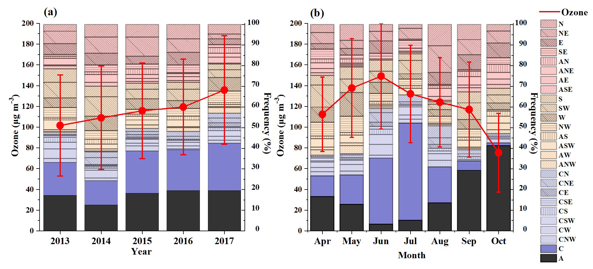
Figure 3Interannual (a) and monthly (b) averaged concentrations of ozone and frequencies of 26 weather types from April to October 2013–2017. The red dots represent the mean values, the vertical red lines indicate the standard deviations, and stacked charts represent the percentages of various weather types (2013 and 2014 are averaged for 14 cities; 2015–2017 are averaged for 58 cities). The pink, orange, light blue, dark blue and black areas represent the weather categories N–E–S direction, S–W–N direction, LP, C and A, respectively.
The monthly mean MDA8 O3 concentrations (Fig. 3b) from April to October were 112, 138, 149, 132, 124, 117 and 75 µg m−3, respectively, and the corresponding exceedance ratios were 9.4 %, 30.1 %, 41.1 %, 26.1 %, 20.3 %, 20.1 % and 3.3 %. The highest domain-averaged MDA8 O3 concentration and exceedance ratio occurred in June, followed by those in May, July, August, September, April and October. Meteorological conditions led to high ozone concentrations in June, and monsoon circulation in July and August resulted in cloudy, rainy conditions and less radiation in the study area (Y. Wang et al., 2009; Tang et al., 2012). The higher ozone concentrations in April than those in October could be associated with strong winds, resulting in a downward transport of ozone due to the lower stratosphere folding mechanism (Stohl and Trickl, 1999; Cooper et al., 2002; Delcloo, 2008; Verstraeten et al., 2015). Notably, this conclusion is different from that of Tang et al. (2012), who reported that the ozone concentration in July was higher than that in May in northern China during 2009–2010. However, as our study indicated that the domain-averaged MDA8 O3 in May was even higher than that in July, the concentrated pollution episode occurred earlier, especially in 2017. The second half of May was the most polluted period, when the exceedance ratio was 46.1 %, which is higher than the ratios observed in the first half of June (39.5 %), the second half of June (45.4 %) and the first half of July (35.6 %). The reason for this difference is probably the abnormally high temperatures in May, especially the second half of May, from 2013 to 2017 and particularly in 2017 (Fig. S2). Many studies have found a strong positive correlation between ozone levels and temperature (Bloomer et al., 2009, 2010; Demuzere et al., 2009; Pusede et al., 2015).
3.2 Weather types and associated surface O3 levels
3.2.1 The meteorological conditions and regional ozone concentrations under different predominant weather types
Based on the Lamb–Jenkinson weather typing technique, 26 circulation patterns affecting northern China were identified, including two vorticity types (anticyclone, A, and cyclone, C), eight directional types (northeasterly, NE; easterly, E; southeasterly, SE; southerly, S; southwesterly, SW; westerly, W; northwesterly, NW; and northerly, N), and 16 hybrids of vorticity and directional types (CN, CNE, CE, CSE, CS, CSW, CW, CNW, AN, ANE, AE, ASE, AS, ASW, AW and ANW). The composite mean sea level pressure maps, along with the occurrence days, are shown in Fig. 4. There are distinctly different locations of the high-pressure and low-pressure centers under the different circulation conditions. The occurrence ratios of vorticity types, pure directional types and hybrid types were 35.6 %, 38.8 % and 25.6 %, respectively, during all 1070 d.

Figure 4Mean surface pressure field (unit: hPa) for the 26 weather types during April–October of 2013–2017 and occurrence days (1070 d in total). “*” indicates the center of northern China.
The midlatitude eastern Eurasian continent is strongly affected by monsoon circulation, and there are several key synoptic systems affecting the circulation and meteorological conditions in northern China. During our study period, northern cyclones (Mongolian and Yellow River cyclones), which are indicative of a low-pressure system located in northwest northern China, dominated in spring and summer. The Siberian High influenced northern China in spring and autumn. The western Pacific subtropical high was also a key system in summer. Therefore, these main synoptic systems resulted in variations in the frequencies of the various weather types in different months over northern China.
Table 1Weather types, ozone concentrations and meteorological conditions for five weather categories.
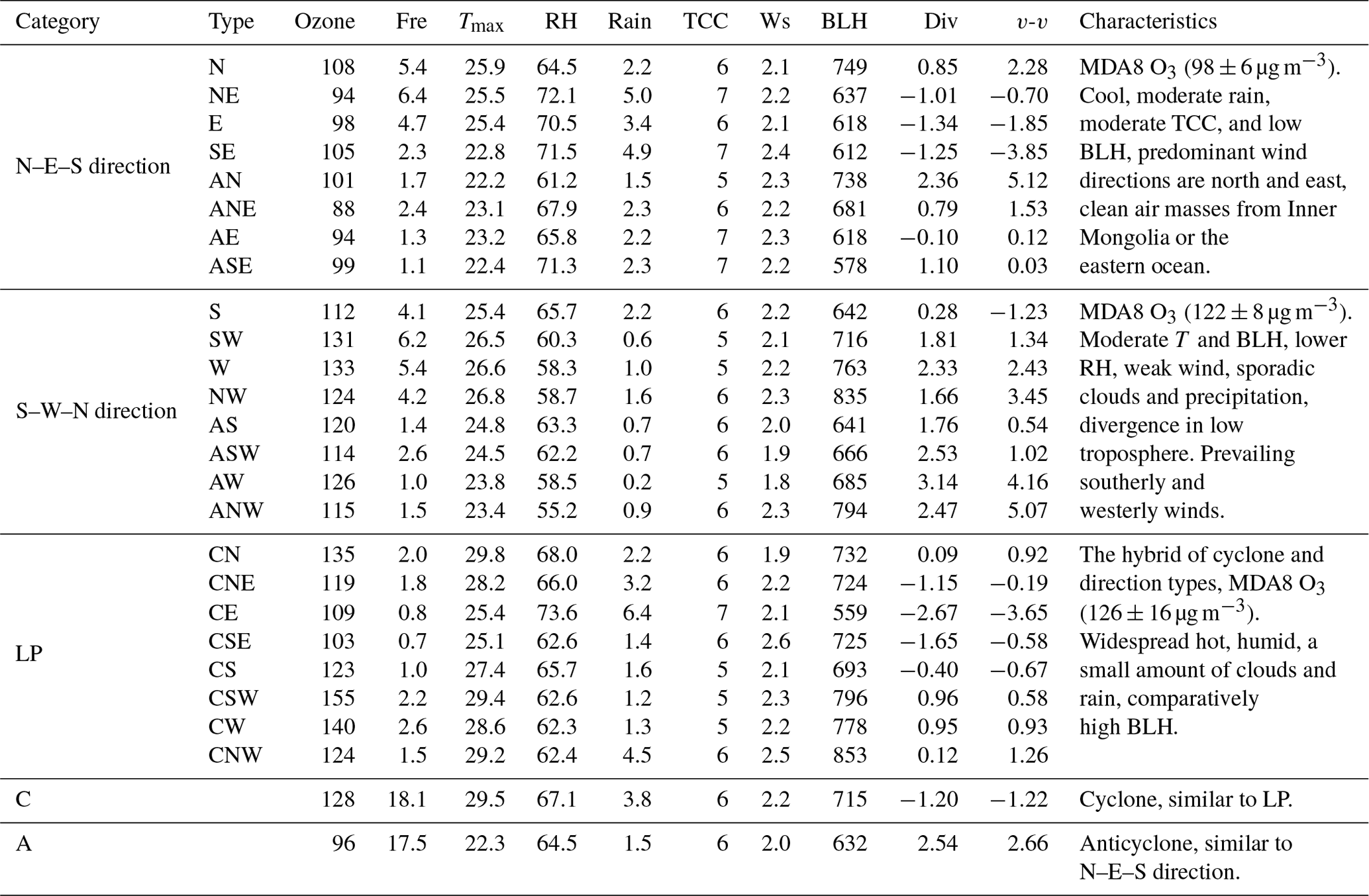
Note: Ozone, MDA8 O3 concentration (µg m−3); fre, frequency of each type (%); Tmax, daily maximum temperature (∘); RH, relative humidity (%); rain, total daily precipitation (mm); TCC, total cloud cover; WS, wind speed (m s−1); BLH, boundary layer height (m); div, divergence of the wind field (10−6 s−1) from 1000 to 850 hPa (seven levels); and v-v, vertical velocity from 1000 to 100 hPa (10−2 Pa s−1).
According to the different locations of the different central systems, together with the similar meteorological factors and mean MDA8 O3 values in these circulation patterns, 26 circulation types were merged into five weather categories: (1) N–E–S direction (geostrophic wind direction diverts from north to south) including N, NE, E, SE, AN, ANE, AE and ASE; (2) S–W–N direction (geostrophic wind direction diverts from south to north) including S, SW, W, NW, AS, ASW, AW and ANE; (3) LP (low-pressure-related weather types) including CN, CNE, CE, CSE, CS, CSW, CW and CNW; (4) A (anticyclone); and (5) C (cyclone). The occurrence ratios of the five weather categories were 25.4 %, 26.5 %, 12.5 %, 17.5 % and 18.1 % in all 1070 d. The predominant local meteorological conditions associated with a specific weather category play an important role in ozone pollution, influencing ozone photoreaction or its regional transport. The values of the averaged MDA8 O3 concentration, frequency of weather types/categories and meteorological variables are depicted in Table 1 and Fig. 5. Briefly, the N–E–S direction and A categories were typically associated with cool and wet air, moderate rain and TCC, low BLH, and relatively clean air masses from the Inner Mongolia/eastern ocean region (Fig. S3); these conditions are unfavorable for ozone formation. Thus, the corresponding area-averaged MDA8 O3 concentrations were 98±6 and 96 µg m−3, respectively. The S–W–N direction category had moderate T and BLH, low RH, weak wind, sporadic clouds and rain, and strong subsidence in the lower troposphere, which contributed to high ozone levels (122±8 µg m−3). The highest ozone concentrations (126±16 and 128 µg m−3) were related to the LP and C categories, which can probably be attributed to the meteorological conditions (hot and humid air, a small amount of TCC and rainfall, and high BLH) that were favorable for ozone formation and transport. However, CE and CSE were different from the other weather types in the LP category, with low O3 concentrations due to low temperatures and easterly winds from the ocean. Overall, the peak values of ozone always occurred in the front of the passage of a cold front or cyclone (most weather types in LP and C), whereas the lowest values occurred during or after the passage of a cold front (most weather types in the N–E–S direction, C with heavy rainfall and CE); similar conclusions were also previously reported (Cooper et al., 2001, 2002; Chen et al., 2008).
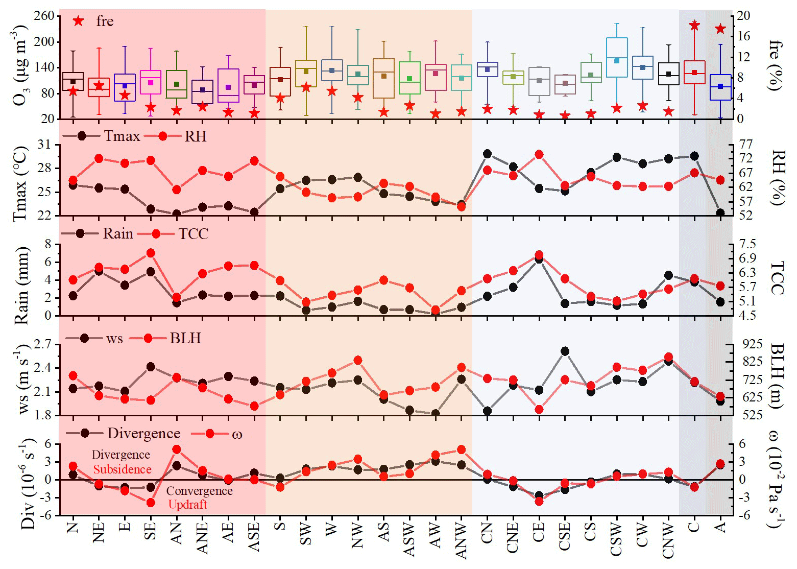
Figure 5Box chart of domain-averaged MDA8 O3 concentrations, occurrence frequency of weather types (fre), and mean values of meteorological factors in 26 weather types during April–October 2013–2017. In the box chart, the solid square indicates the mean, the horizontal lines across the box are the averages of the first, median, and third quartiles, respectively, and the lower and upper whiskers represent the 5th and 95th percentiles, respectively. The pink, orange, light blue, dark blue and black areas represent the weather categories N–E–S direction, S–W–N direction, LP (low-pressure-related weather patterns), C (cyclone) and A (anticyclone), respectively.
3.2.2 Spatial distributions of the 26 weather types/five categories
The spatial distribution of the averaged MDA8 O3 concentration under different weather types is shown in Fig. 6, and Figs. S3–S7 display the spatial distributions of the combined wind field with BLH, maximum temperature (Tmax), RH, rain and TCC, respectively. In most cities, the lowest MDA8 O3 concentrations occurred in the N–E–S direction and A weather categories. The S–W–N direction category, having predominantly southerly winds throughout the region or south of northern China, exhibited high ozone values along with the prevailing wind direction. The LP and C weather categories, having the highest regional averaged levels, were associated with high Tmax and strong southerly flow, moderate RH and ample sunshine, which are the meteorological conditions that are favorable for ozone formation as well as the transport of ozone and its precursors from polluted areas.
3.2.3 Interannual and monthly ozone variation elaborated from the perspective of circulation pattern changes
The interannual or monthly ozone concentration changes are associated with variations in weather types. Figure 3 indicates that the ratios of high-ozone weather categories (S–W–N direction, LP and C S–W–N direction, LP and C) were most frequent in 2013 and 2017, less frequent in 2015 and 2016, and least frequent in 2014. The high-ozone weather categories accounted for 61.5 % and 61.8 % of the time in 2013 and 2017, respectively. Under similar weather conditions, low ozone levels could also be associated with high PM2.5 levels in 2013 and 2015. The contributions of frequency-only and circulation changes (frequency and intensity) to the interannual ozone variability will be discussed in Sect. 3.3.
Due to the impacts by monsoon circulation systems, the frequencies of weather types varied dramatically on a monthly scale (Fig. 3b). The frequencies of both the N–E–S direction and A gradually decreased in spring, whereas the frequencies of the S–W–N direction, LP and C gradually increased. In autumn, the frequencies of LP and C decreased, whereas those of the S–W–N direction, N–E–S direction and A increased. The weather categories C and LP dominated in summer. The high-ozone weather categories (S–W–N direction, LP and C) accounted for 58.7 %, 66.5 %, 79.3 %, 80.6 %, 49.0 %, 38.0 % and 27.7 % of the time in the months from April to October, respectively. These frequencies were highest in July, June and May, which probably resulted in the highest monthly averaged regional ozone concentrations. However, due to the influence of monsoon circulation, large amounts of rainfall occurred during July: 73 out of 194 d during the 5 years were rainy in category C, which reduced the ozone levels. Notably, severe ozone pollution in May, especially in the second half of May in 2017, was closely related to abnormally high frequencies under the control of the most polluted synoptic categories (LP and C), accounting for 35.5 % in 31 d and 50.0 % in 16 d (Table S2). With the development of the Siberian High from August to October, the N–E–S direction and A weather categories occurred frequently, and the monthly averaged ozone concentrations declined.
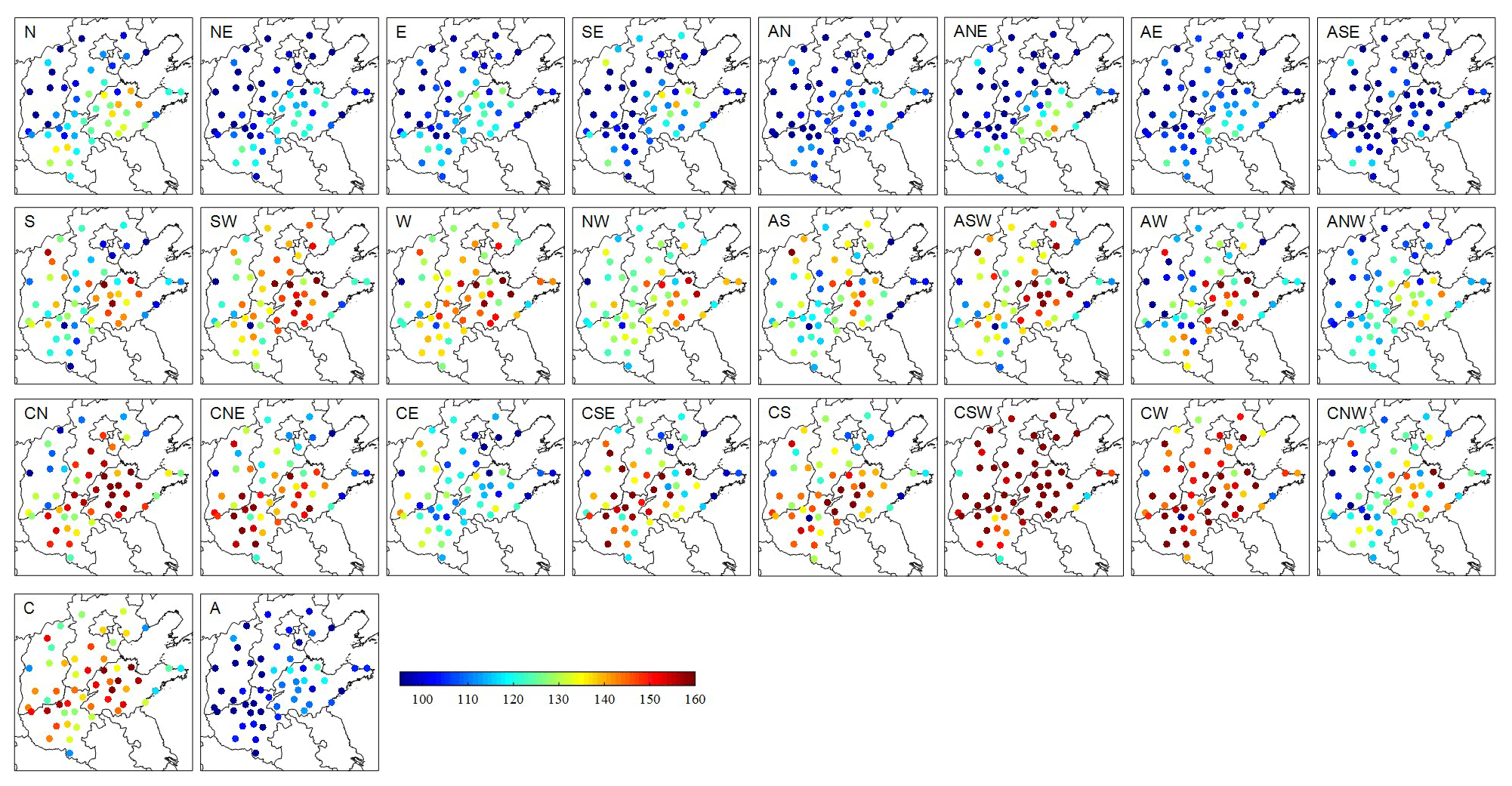
Figure 6Spatial distribution of average MDA8 O3 for the 26 weather types. The first, second and third rows correspond to the weather categories N–E–S direction, S–W–N direction and LP, respectively, and the fourth row includes both categories C and A.
3.3 Effects of synoptic changes on interannual ozone variability
3.3.1 Effect of weather type intensity on interannual ozone variability
The pressure fields for the 26 synoptic types per year from 2013 to 2017 (Figs. S8–S9) indicated that every synoptic weather type varied in both frequency and intensity. The intensity of the circulation patterns indicated the differences in the center pressure, the location of the predominant system, the pressure gradient and the domain-averaged sea level pressure. The correlations between ECII and ΔO3 (as introduced in Sect. 2.4) differed in the different circulation types in the various cities. For instance, the strong negative correlation between these two variables for weather type C in ZJK (Fig. 7a) indicated that the low values of min slp were associated with high MDA8 O3 concentrations.
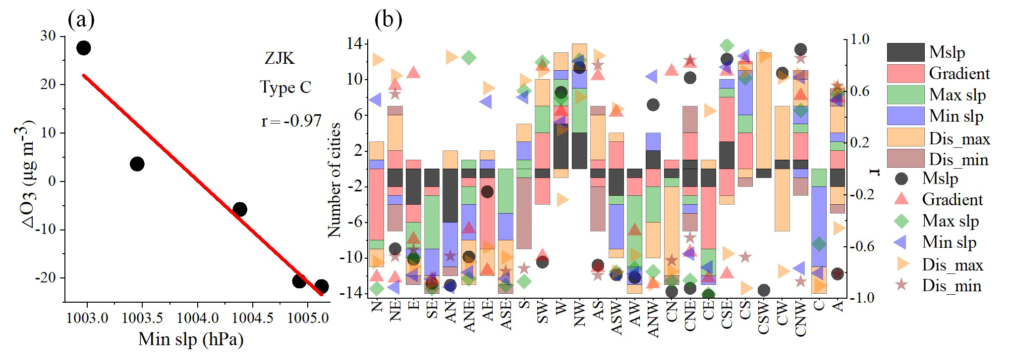
Figure 7Scatterplot of ΔO3 versus min slp for weather type C in ZJK (a). The red line represents the linear fitting between min slp (the ECII under weather type C in ZJK) and ΔO3 (the difference between the MDA8 O3 for a given year and the corresponding 5-year average); r represents the correlation coefficient. The number of cities (histogram) and averaged correlation coefficient r (points of different shapes) according to corresponding ECII under each weather type among 14 cities (b). The number of cities with positive or negative values represents positive or negative correlations between ECII and ΔO3. For example, under CW controls, there are one, six and seven cities where ECII corresponds to mslp with a positive correlation, dis max with a positive correlation and dis max with a negative correlation, respectively, and the average r is 0.74, 0.70 and −0.79, respectively.
The number of cities and averaged r values according to the corresponding ECII under each circulation type among the 14 cities are shown in Fig. 7b. Overall, the average absolute value of r was 0.74. For circulation type C, ΔO3 was strongly correlated with min slp in nine of the cities, and the average r was −0.81, i.e., a strong negative correlation. A strong negative correlation between ΔO3 and the pressure gradient was evident for circulation type N, whereas an opposite pattern occurred for circulation types CSE and CS. The reasons for this difference are as follows. Northerly winds prevailed for circulation type N, and high-pressure gradients indicated strong northerly winds that brought clean air masses from the north, which resulted in a decrease in the MDA8 O3 concentration. However, high temperatures and RH as well as prevailing southerly or easterly winds (Figs. S3–S5) occurred in southern cities in the CSE and CS circulation types. In addition, the abundance of precursors and ozone in the upwind region facilitated ozone formation and transport with the increasing pressure gradient (wind speeds).
Even under the same weather type controls, the ECII and the values of r differed in the different cities. This phenomenon was caused by differences in geographic location, topographic discrepancies and the properties of the upwind air mass. Therefore, under the control of the same weather type, the ECII was the same in adjacent cities.
3.3.2 Quantifying the effects of the interannual synoptic changes on the interannual ozone variability
Based on Eqs. (1) and (2), we reconstructed the interannual ozone levels by taking into account either frequency-only or both frequency and intensity variations in synoptic circulations, which are and , respectively. The differences between the maximum and minimum annual reconstructed ozone are labeled as and , respectively. ΔO3_obs differed between the maximum and minimum for the annual observed O3 concentration. Thus, the contributions of interannual variability in O3 influenced by frequency-only and frequency and intensity variations in synoptic circulation were _obs and _obs, respectively, which indicate the interannual oscillations in ozone levels caused by synoptic variability.
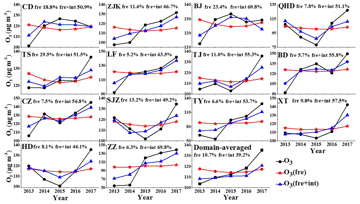
Figure 8The interannual MDA8 O3 concentration trends for observed and reconstructed O3 based on variations in weather types in 14 cities. The black lines represent the observed interannual MDA8 O3 trend, whereas the red and blue lines are the trends of reconstructed MDA8 O3 concentrations according to the frequency-only and both frequency and intensity of weather type changes, respectively. The percentages in each city indicate the O3 interannual variabilities influenced by frequency-only and by both frequency and intensity of weather type changes.
The observed and reconstructed (influenced by frequency-only and frequency and intensity variations in synoptic circulations) interannual MDA8 O3 levels for 5 years in 14 cities and the whole region are shown in Fig. 8. The contributions of interannual variability in O3 influenced by frequency and intensity variations in synoptic circulation ranged from 44.1 % to 69.8 % over the 14 cities, and the contributions by frequency-only variations ranged from 5.2 % to 23.4 %. Obviously, the interannual fluctuations in the ozone concentration were caused mainly by weather type intensity changes in northern China. In addition, based on the regional averaged scale, the interannual variability in the domain-averaged observed MDA8 O3 in 14 cities varied from averaged maximum values of 135 µg m−3 in 2017 to a minimum of 104 µg m−3 in 2013. The contributions of variations in circulation patterns to interannual O3 increases were 39.2 %, and the remaining interannual variability was possibly due to nonlinear relationships resulting from recent emission control measures over northern China.
In most cities, the contributions of synoptic circulation changes on ozone variability obtained here (44.1 %–69.8 %) are higher than those (50 %) estimated by Zhang et al. (2013). The difference could be attributed to our results being based on (1) more weather types, (2) weather types covering all days and (3) more CIIs, which can better characterize the intensity of slp. Furthermore, a higher contribution in a single city and increasing reconstructed ozone indicate that synoptic circulation patterns play an important role in the ozone variability in northern China. However, our regional contribution (39.2 %) is lower than that (46 %) estimated by Hegarty et al. (2007), which reveals that the increasing trend of ozone concentrations from 2013 to 2017 in northern China is largely associated with the impact of its precursors.
3.4 Quantifying the impact of weather patterns on day-to-day ozone concentration and forecasting daily ozone concentration
Based on the five weather categories defined in Sect. 3.2.1, a segmented synoptic-regression analysis approach (introduced in Sect. 2.5) was established to quantify the impact of weather patterns on the day-to-day ozone concentration and to construct the ozone potential forecast model.
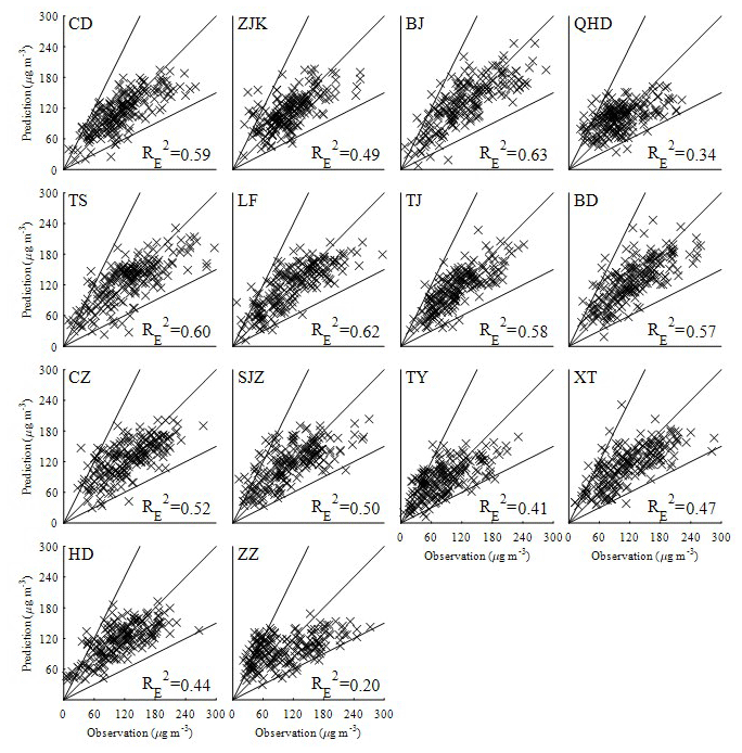
Figure 9Scatterplots of predicted versus observed MDA8 O3 concentrations for each city. The predicted concentrations were obtained by inputting the validation data (20 % of the total data) into the corresponding model equations for five weather categories. The values indicate the percentage of explained variance in the composite model that contains the building and validation datasets for each city. The three black lines indicate 2:1, 1:1 and 1:2 ratio lines of predictions and observations.
The contributions of local meteorological factors to the day-to-day variations in ozone can be evaluated by the explained variance () calculated from the synoptic-regression-based models (Hien et al., 2002; W. T. Wang et al., 2009). Overall, the predicted versus observed MDA8 O3 concentrations for the validation data are shown in Fig. 9; the predicted concentrations were obtained by inputting the validation data (the part that was not used to build the model, which was 20 % of the total data) into the corresponding model equations for the five weather categories for each city. Local meteorological parameters explained 57 %–63 % and 41 %–52 % of the day-to-day variability in the MDA8 O3 concentration for the northern cities (except for QHD, 34 %) and southern cities (except for ZZ, 20 %), respectively.
Table 2All parameters used in the stepwise regression and the number of cities (out of 14) for which each variable was selected for each weather category.
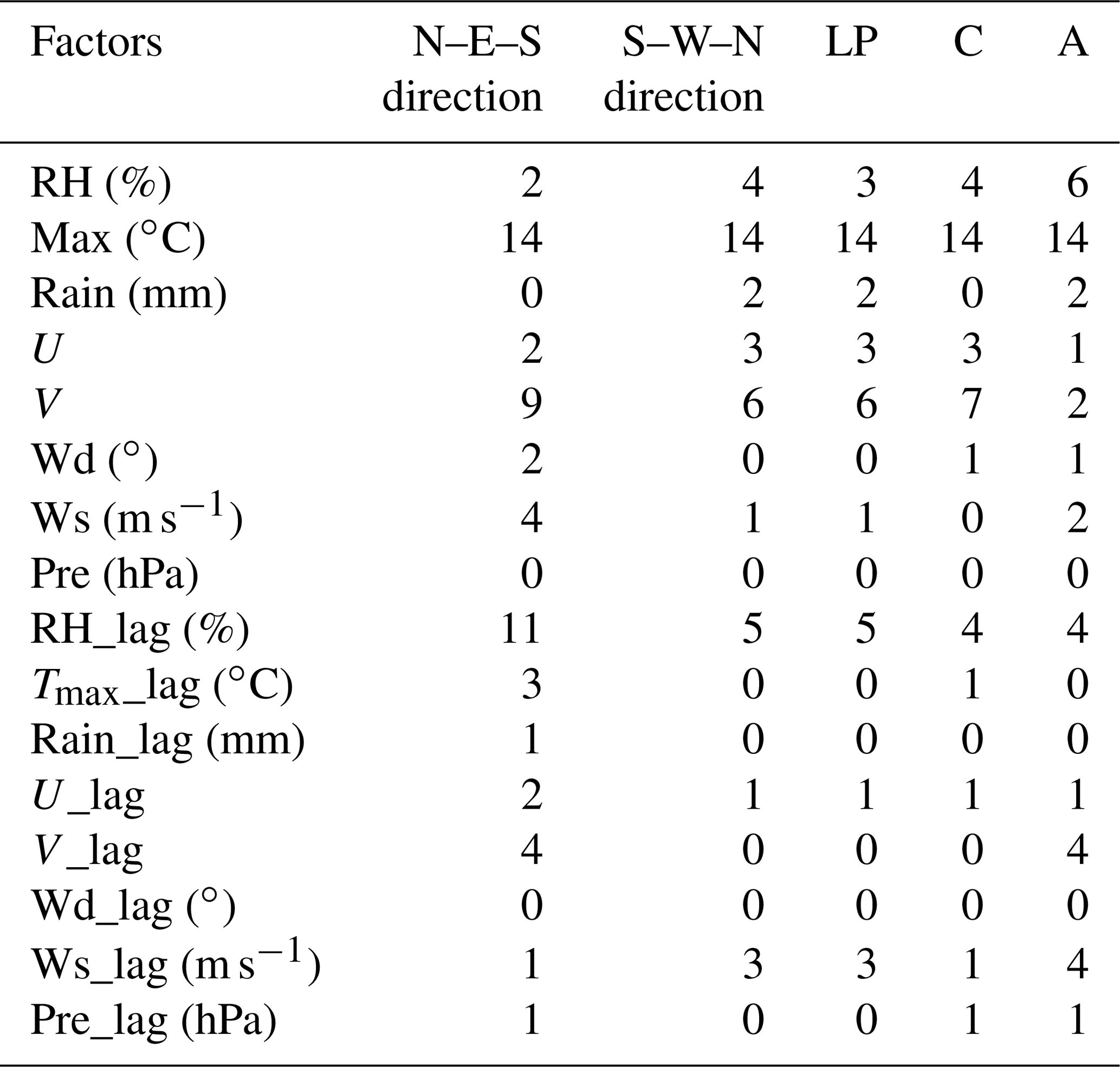
Note: RH, Tmax, rain, U, V, wd, ws and pre are relative humidity, maximum temperature, precipitation, u component, v component, wind direction, wind speed and pressure, respectively. The suffix “lag” means the meteorological factors from the previous day.
In addition, the results of segmented synoptic-regression analysis in 14 cities, i.e., the daily MDA8 O3 potential forecast equations for each category in each city, are shown in Table S3. Table 2 represents the number of cities (14 total) from which the meteorological factors were used in a stepwise regression model under each weather category. The results show that Tmax exhibited a strong positive correlation with ozone; thus, this factor is the primary influencing factor in all categories and all cities, as high temperatures are related to high ozone concentrations in northern China. V exhibited a positive correlation with O3 in the northern part of this region (at the north–south boundary at approximately 38.5∘ N), which means that southerly flow caused an increase in the ozone concentration. Therefore, as discussed in Sect. 3.2.2, high temperatures and southerly winds were the main factors that contributed to increased ozone concentrations in northern China from a regional perspective. Both RH_lag and RH showed a negative correlation with O3, and the former had more occurrences and greater weights in the equations than the latter. This phenomenon may exist because RH of approximately 40 %–50 % (Zhao et al., 2019) generates more hydroxyl radicals (OH), facilitating ozone formation, and ozone is stored in the residual layer and transported to the surface the next day via convection and diffusion. In addition, TCC is a key factor.
Three statistical measures (R2, RMSE and CV) for the building and validation datasets for the five weather categories and the composite model, which integrates the five weather categories, in the 14 cities (Table S4) indicate that the potential forecast equations for MDA8 O3 were acceptable in most cities. Scatterplots of predicted versus observed MDA8 O3 concentrations in the composite validation datasets in each city are shown in Fig. 9. For the validation data, the prediction of ozone concentration was obtained by inputting the meteorological factors into the simulated formula for the corresponding weather category in each city; therefore, the composite validation datasets indicated the integrated predicted ozone concentrations for the five categories. The results of validation show that R2 was higher than 0.50, except for QHD, Shijiazhuang (SJZ) and ZZ (0.24–0.47), while CV was lower than 40 %, except for Taiyuan (TY) and ZZ.
The results reveal that most of the validation data are within the acceptable error range, as they are concentrated within the 2:1 and 1:2 ratio lines, and the scatters are distributed evenly around the 1:1 line. For example, the comparison of the observed and predicted ozone in Beijing during our study period is shown in Fig. S10. This finding also indicates that the segmented synoptic-regression approach is practical for constructing ozone potential forecasting models in most cities in northern China.
In brief, the aforementioned results can provide references for daily MDA8 O3 prediction for each city and facilitate the understanding and evaluation of the impact of local meteorology on daily ozone variations on an urban scale.
In this study, we demonstrated the interannual and monthly variations in the surface MDA8 O3 concentration in northern China during April–October 2013–2017, investigated the relationship between weather types and MDA8 O3 levels, quantified the contributions of weather types and local variations in meteorological factors to both the interannual and day-to-day variability in ozone, and built ozone potential forecast equations. The main results are as follows.
-
The annual domain-averaged concentrations of MDA8 O3 during 2013–2017 were 102, 109, 116, 119 and 136 µg m−3, respectively, and the highest exceedance ratio (31.1 %) was observed in 2017. The monthly mean MDA8 O3 concentrations were 112, 138, 149, 132, 124, 117 and 75 µg m−3 from April to October, respectively, with a significantly increasing rate of 0.87 µg m−3 month−1 during the 5-year period. The most polluted cities were concentrated around Beijing, the southeast of Hebei, and the west and north of Shandong.
-
A total of 26 weather types were objectively identified based on the Lamb–Jenkinson method and combined into five weather categories according to similar meteorological factors and MDA8 O3 concentrations. The high ozone levels in 2017 and during May–July were partly due to the high frequency of the highly polluted weather categories (S–W–N direction, LP and C) resulting from high temperatures, moderate RH and southerly air flows.
-
The intensity of synoptic circulation patterns was the dominant factor through which variations in weather types influenced the variability in the ozone levels. The contributions of interannual variability in O3 influenced by both frequency and intensity variations in synoptic circulation patterns ranged from 44 % to 70 % over the 14 cities that were evaluated in detail, whereas the contributions of the variations in circulation patterns to the increase in the interannual O3 from 2013 to 2017 was only 39.2 % based on a regionally averaged scale.
-
The results of the daily ozone potential forecast equations in the 14 cities showed that high temperatures, moderate RH and southerly winds could result in severe ozone pollution in the northern part of northern China, whereas the southern part was mainly affected by high temperatures and RH. Local meteorological parameters explained 55 %–64 % and 43 %–49 % of the day-to-day MDA8 O3 variability for the northern cities (except for QHD, 32 %) and southern cities (except for ZZ, 25 %), respectively.
The daily average mass concentrations of ozone were obtained from the National Urban Air Quality Real-time Publishing Platform (http://106.37.208.233:20035/, last access: 15 October 2019) issued by the Chinese Ministry of Ecology and Environment. Daily meteorological data were obtained from the China Meteorological Administration in the Meteorological Information Combine Analysis and Process System (MICAPS), and daily meteorological reanalysis data (gridded at 1∘ × 1∘) were obtained from ERA-Interim (https://apps.ecmwf.int/datasets/data/interim-full-daily/levtype=sfc/, last access: 1 November 2019). All of the data can be obtained upon request.
The supplement related to this article is available online at: https://doi.org/10.5194/acp-19-14477-2019-supplement.
LW designed this research. JL and LW interpreted the data and wrote the paper. ML processed some of the data. The weather type classification program was provided by ZL. YS, TS and WG provided some of the PM2.5 and O3 data. YL provided some of the meteorological data. All of the authors commented on the paper.
The authors declare that they have no conflict of interest.
We give special thanks to the National Earth System Science, Data Sharing Infrastructure, and the National Science & Technology Infrastructure of China. We also thank ECMWF for providing daily ERA-Interim reanalysis data in our work.
This work was partially supported by grants from the National Key R&D Plan (Quantitative Relationship and Regulation Principle between Regional Oxidation Capacity of Atmospheric and Air Quality 2017YFC0210003), the National Natural Science Foundation of China (nos. 41505133 & 41775162), the Strategic Priority Research Program of the Chinese Academy of Sciences (no. XDA19020303), the National Research Program for Key Issues in Air Pollution Control (DQGG0101), Beijing Major Science and Technology Project 510 (Z181100005418014), the Postgraduate Research & Practice Innovation Program of Jiangsu Province (no. 1344051901061) and the China Scholarship Council Fellowship (201804910025).
This paper was edited by Min Shao and reviewed by two anonymous referees.
Barrero, M. A., Grimalt, J. O., and Cantón, L.: Prediction of daily ozone concentration maxima in the urban atmosphere, Chemometr. Intell. Lab., 80, 67–76, https://doi.org/10.1016/j.chemolab.2005.07.003, 2006.
Bloomer, B. J., Stehr, J. W., Piety, C. A., Salawitch, R. J., and Dickerson, R. R.: Observed relationships of ozone air pollution with temperature and emissions, Geophys. Res. Lett., 36, 269–277, 2009.
Bloomer, B. J., Vinnikov, K. Y., and Dickerson, R. R.: Changes in seasonal and diurnal cycles of ozone and temperature in the eastern U.S, Atmos. Environ., 44, 2543–2551, 2010.
Chan, C. K. and Yao, X.: Air pollution in mega cities in China, Atmos. Environ., 42, 1–42, https://doi.org/10.1016/j.atmosenv.2007.09.003, 2008.
Chen, Z. H., Cheng, S. Y., Li, J. B., Guo, X. R., Wang, W. H., and Chen, D. S.: Relationship between atmospheric pollution processes and synoptic pressure patterns in northern China, Atmos. Environ., 42, 6078–6087, https://doi.org/10.1016/j.atmosenv.2008.03.043, 2008.
Comrie, A. C. and Yarnal, B.: Relationships between synoptic-scale atmospheric circulation and ozone concentrations in Metropolitan Pittsburgh, Pennsylvania, Atmos. Environ. B-Urb., 26, 301–312, 1992.
Conway, D. and Jones, P. D.: The use of weather types and air flow indices for GCM downscaling, J. Hydrol., 212–213, 348–361, https://doi.org/10.1016/S0022-1694(98)00216-9, 1998.
Cooper, O. R., Moody, J. L., Parrish, D. D., Trainer, M., Ryerson, T. B., Holloway, J. S., Hübler, G., Fehsenfeld, F. C., Oltmans, S. J., and Evans, M. J.: Trace gas signatures of the airstreams within North Atlantic cyclones: Case studies from the North Atlantic Regional Experiment (NARE '97) aircraft intensive, J. Geophys. Res.-Atmos., 106, 5437–5456, https://doi.org/10.1029/2000jd900574, 2001.
Cooper, O. R., Moody, J. L., Parrish, D. D., Trainer, M., Holloway, J. S., Hübler, G., Fehsenfeld, F. C., and Stohl, A.: Trace gas composition of midlatitude cyclones over the western North Atlantic Ocean: A seasonal comparison of O3 and CO, J. Geophys. Res.-Atmos., 107, ACH 2-1-ACH 2-12, https://doi.org/10.1029/2001jd000902, 2002.
Delcloo, A. W. and H. De Backer: Five day 3D back trajectory clusters and trends analysis of the Uccle ozone sounding time series in the lower troposphere (1969–2001), Atmos. Environ., 42, 4419–4432, 2008.
Demuzere, M. and van Lipzig, N. P. M.: A new method to estimate air-quality levels using a synoptic-regression approach, Part I: Present-day O3 and PM10 analysis, Atmos. Environ., 44, 1341–1355, https://doi.org/10.1016/j.atmosenv.2009.06.029, 2010.
Demuzere, M., Trigo, R. M., Vila-Guerau de Arellano, J., and van Lipzig, N. P. M.: The impact of weather and atmospheric circulation on O3 and PM10 levels at a rural mid-latitude site, Atmos. Chem. Phys., 9, 2695–2714, https://doi.org/10.5194/acp-9-2695-2009, 2009.
Eder, B. K., Davis, J. M., and Bloomfield, P.: An Automated Classification Scheme Designed to Better Elucidate the Dependence of Ozone on Meteorology, J. Appl. Meteorol., 33, 1182–1199, 1994.
Fleming, Z. L., Doherty, R. M., Von Schneidemesser, E., Malley, C. S., Cooper, O. R., Pinto, J. P., Colette, A., Xu, X., Simpson, D., Schultz, M. G., Lefohn, A. S., Hamad, S., Moolla, R., Solberg, S., and Feng, Z.: Tropospheric Ozone Assessment Report: Present-day ozone distribution and trends relevant to human health, Elem. Sci. Anth., 6, 12, https://doi.org/10.1525/elementa.273, 2018.
He, J., Yu, Y., Xie, Y., Mao, H., Wu, L., Liu, N., and Zhao, S.: Numerical Model-Based Artificial Neural Network Model and Its Application for Quantifying Impact Factors of Urban Air Quality, Water Air Soil Pollut., 227–235, https://doi.org/10.1007/s11270-016-2930-z, 2016.
He, J., Gong, S., Yu, Y., Yu, L., Wu, L., Mao, H., Song, C., Zhao, S., Liu, H., Li, X., and Li, R.: Air pollution characteristics and their relation to meteorological conditions during 2014–2015 in major Chinese cities, Environ. Pollut., 223, 484–496, https://doi.org/10.1016/j.envpol.2017.01.050, 2017.
Hegarty, J., Mao, H., and Talbot, R.: Synoptic controls on summertime surface ozone in the northeastern United States, J. Geophys. Res., 112, D14306, https://doi.org/10.1029/2006jd008170, 2007.
Hien, P. D., Bac, V. T., Tham, H. C., Nhan, D. D., and Vinh, L. D.: Influence of meteorological conditions on PM2.5 and PM2.5−10 concentrations during the monsoon season in Hanoi, Vietnam, Atmos. Environ., 36, 3473–3484, https://doi.org/10.1016/s1352-2310(02)00295-9, 2002.
Jacob, D. J. and Winner, D. A.: Effect of climate change on air quality, Atmos. Environ., 43, 51–63, https://doi.org/10.1016/j.atmosenv.2008.09.051, 2009.
Kinney, P. L.: Climate change, air quality, and human health, Am. J. Prev. Med., 35, 459–467, https://doi.org/10.1016/j.amepre.2008.08.025, 2008.
Lamb, H.: British Isles weather types and a register of the daily sequence of circulation patterns, Geophys. Mem, 116, 1861–1971, 1972.
Li, K., Jacob, D. J., Liao, H., Shen, L., Zhang, Q., and Bates, K. H.: Anthropogenic drivers of 2013–2017 trends in summer surface ozone in China, P. Natl. Acad. Sci. USA, 116, 422–427, https://doi.org/10.1073/pnas.1812168116, 2019.
Liao, Z., Gao, M., Sun, J., and Fan, S.: The impact of synoptic circulation on air quality and pollution-related human health in the Yangtze River Delta region, Sci. Total Environ., 607–608, 838–846, https://doi.org/10.1016/j.scitotenv.2017.07.031, 2017.
Liu, Y., Franklin, M., Kahn, R., and Koutrakis, P.: Using aerosol optical thickness to predict ground-level PM2.5 concentrations in the St. Louis area: A comparison between MISR and MODIS, Remote Sens. Environ., 107, 33–44, https://doi.org/10.1016/j.rse.2006.05.022, 2007.
Liu, Y., He, K. B., Li, S. S., Wang, Z. X., Christiani, D. C., and Koutrakis, P.: A statistical model to evaluate the effectiveness of PM2.5 emissions control during the Beijing 2008 Olympic Games, Environ. Int., 44, 100–105, https://doi.org/10.1016/j.envint.2012.02.003, 2012.
Lu, X., Hong, J., Zhang, L., Cooper, O. R., and Zhang, Y.: Severe Surface Ozone Pollution in China: A Global Perspective, Environ. Sci. Tech. Lett., 5, 487–494, 2018.
Lu, X., Zhang, L., Chen, Y., Zhou, M., Zheng, B., Li, K., Liu, Y., Lin, J., Fu, T.-M., and Zhang, Q.: Exploring 2016–2017 surface ozone pollution over China: source contributions and meteorological influences, Atmos. Chem. Phys., 19, 8339–8361, https://doi.org/10.5194/acp-19-8339-2019, 2019.
Mckendry, I. G., Stahl, K., and Moore, R. D.: Synoptic sea-level pressure patterns generated by a general circulation model: comparison with types derived from NCEP/NCAR re-analysis and implications for downscaling, International J. Climatol., 26, 1727–1736, 2006.
Mills, G., Pleijel, H., Malley, C. S., Sinha, B., Cooper, O. R., Schultz, M. G., Neufeld, H. S., Simpson, D., Sharps, K., Feng, Z., Gerosa, G., Harmens, H., Kobayashi, K., Saxena, P., Paoletti, E., Sinha, V., and Xu, X.: Tropospheric Ozone Assessment Report: Present-day tropospheric ozone distribution and trends relevant to vegetation, Elem. Sci. Anth., 6–47, https://doi.org/10.1525/elementa.302, 2018.
Monks, P. S., Granier, C., Fuzzi, S., Stohl, A., Williams, M. L., Akimoto, H., Amann, M., Baklanov, A., Baltensperger, U., Bey, I., Blake, N., Blake, R. S., Carslaw, K., Cooper, O. R., Dentener, F., Fowler, D., Fragkou, E., Frost, G. J., Generoso, S., Ginoux, P., Grewe, V., Guenther, A., Hansson, H. C., Henne, S., Hjorth, J., Hofzumahaus, A., Huntrieser, H., Isaksen, I. S. A., Jenkin, M. E., Kaiser, J., Kanakidou, M., Klimont, Z., Kulmala, M., Laj, P., Lawrence, M. G., Lee, J. D., Liousse, C., Maione, M., McFiggans, G., Metzger, A., Mieville, A., Moussiopoulos, N., Orlando, J. J., O'Dowd, C. D., Palmer, P. I., Parrish, D. D., Petzold, A., Platt, U., Pöschl, U., Prévôt, A. S. H., Reeves, C. E., Reimann, S., Rudich, Y., Sellegri, K., Steinbrecher, R., Simpson, D., ten Brink, H., Theloke, J., van der Werf, G. R., Vautard, R., Vestreng, V., Vlachokostas, C., and von Glasow, R.: Atmospheric composition change – global and regional air quality, Atmos. Environ., 43, 5268–5350, https://doi.org/10.1016/j.atmosenv.2009.08.021, 2009.
Monks, P. S., Archibald, A. T., Colette, A., Cooper, O., Coyle, M., Derwent, R., Fowler, D., Granier, C., Law, K. S., Mills, G. E., Stevenson, D. S., Tarasova, O., Thouret, V., von Schneidemesser, E., Sommariva, R., Wild, O., and Williams, M. L.: Tropospheric ozone and its precursors from the urban to the global scale from air quality to short-lived climate forcer, Atmos. Chem. Phys., 15, 8889–8973, https://doi.org/10.5194/acp-15-8889-2015, 2015.
Moody, J. L., Munger, J. W., Goldstein, A. H., Jacob, D. J., and Wofsy, S. C.: Harvard Forest regional-scale air mass composition by Patterns in Atmospheric Transport History (PATH), J. Geophys. Res.-Atmos., 103, 13181–13194, https://doi.org/10.1029/98jd00526, 1998.
Pope, R. J., Butt, E. W., Chipperfield, M. P., Doherty, R. M., Fenech, S., Schmidt, A., Arnold, S. R., and Savage, N. H.: The impact of synoptic weather on UK surface ozone and implications for premature mortality, Environ. Res. Lett., 11, 124004, https://doi.org/10.1088/1748-9326/11/12/124004, 2016.
Pusede, S. E., Steiner, A. L., and Cohen, R. C.: Temperature and Recent Trends in the Chemistry of Continental Surface Ozone, Chem. Rev., 115, 3898–3918, https://doi.org/10.1021/cr5006815, 2015.
Robeson, S. M. and Steyn, D. G.: Evaluation and comparison of statistical forecast models for daily maximum ozone concentrations, Atmos. Environ. B-Urb., 24, 303–312, 1990.
Russo, A., Trigo, R. M., Martins, H., and Mendes, M. T.: NO2, PM10 and O3 urban concentrations and its association with circulation weather types in Portugal, Atmos. Environ., 89, 768–785, https://doi.org/10.1016/j.atmosenv.2014.02.010, 2014.
Santurtún, A., González-Hidalgo, J. C., Sanchez-Lorenzo, A., and Zarrabeitia, M. T.: Surface ozone concentration trends and its relationship with weather types in Spain (2001–2010), Atmos. Environ., 101, 10–22, 2015.
Shen, L., Mickley, L. J., and Tai, A. P. K.: Influence of synoptic patterns on surface ozone variability over the eastern United States from 1980 to 2012, Atmos. Chem. Phys., 15, 10925–10938, https://doi.org/10.5194/acp-15-10925-2015, 2015.
Stohl, A. and Trickl, T.: A textbook example of long-range transport: Simultaneous observation of ozone maxima of stratospheric and North American origin in the free troposphere over Europe, J. Geophys. Res.-Atmos., 104, 30445–30462, 1999.
Tang, G., Wang, Y., Li, X., Ji, D., Hsu, S., and Gao, X.: Spatial-temporal variations in surface ozone in Northern China as observed during 2009–2010 and possible implications for future air quality control strategies, Atmos. Chem. Phys., 12, 2757–2776, https://doi.org/10.5194/acp-12-2757-2012, 2012.
Trigo, R. M. and Dacamara, C. C.: Circulation weather types and their influence on the precipitation regime in Portugal, Int. J. Climatol., 20, 1559–1581, 2000.
Verstraeten, W. W., Neu, J. L., Williams, J. E., Bowman, K. W., Worden, J. R., and Boersma, K. F.: Rapid increases in tropospheric ozone production and export from China, Nat. Geosci., 8, 690–695, https://doi.org/10.1038/ngeo2493, 2015.
Wang, T., Wei, X. L., Ding, A. J., Poon, C. N., Lam, K. S., Li, Y. S., Chan, L. Y., and Anson, M.: Increasing surface ozone concentrations in the background atmosphere of Southern China, 1994–2007, Atmos. Chem. Phys., 9, 6217–6227, https://doi.org/10.5194/acp-9-6217-2009, 2009.
Wang, W. T., Primbs, T., Tao, S., and Simonich, S. L. M.: Atmospheric Particulate Matter Pollution during the 2008 Beijing Olympics, Environ. Sci. Technol., 43, 5314–5320, https://doi.org/10.1021/es9007504, 2009.
Wang, Y., Hao, J., McElroy, M. B., Munger, J. W., Ma, H., Chen, D., and Nielsen, C. P.: Ozone air quality during the 2008 Beijing Olympics: effectiveness of emission restrictions, Atmos. Chem. Phys., 9, 5237–5251, https://doi.org/10.5194/acp-9-5237-2009, 2009.
Yarnal, B.: Synoptic Climatology in Environmental Analysis A Primer, J. Prevent. Med. Info., 347, 170–180, 1993.
Zhang, J. P., Zhu, T., Zhang, Q. H., Li, C. C., Shu, H. L., Ying, Y., Dai, Z. P., Wang, X., Liu, X. Y., Liang, A. M., Shen, H. X., and Yi, B. Q.: The impact of circulation patterns on regional transport pathways and air quality over Beijing and its surroundings, Atmos. Chem. Phys., 12, 5031–5053, https://doi.org/10.5194/acp-12-5031-2012, 2012.
Zhang, Y., Mao, H., Ding, A., Zhou, D., and Fu, C.: Impact of synoptic weather patterns on spatio-temporal variation in surface O3 levels in Hong Kong during 1999–2011, Atmos. Environ., 73, 41–50, https://doi.org/10.1016/j.atmosenv.2013.02.047, 2013.
Zhao, W., Tang, G., Yu, H., Yang, Y., Wang, Y., Wang, L., An, J., Gao, W., Hu, B., Cheng, M., An, X., Li, X., and Wang, Y.: Evolution of boundary layer ozone in Shijiazhuang, a suburban site on the North China Plain, J. Environ. Sci., 83, 152–160, https://doi.org/10.1016/j.jes.2019.02.016, 2019.