the Creative Commons Attribution 4.0 License.
the Creative Commons Attribution 4.0 License.
Development and application of observable response indicators for design of an effective ozone and fine-particle pollution control strategy in China
Jia Xing
Dian Ding
Zhaoxin Dong
James T. Kelly
Carey Jang
Yun Zhu
Jiming Hao
Designing effective control policies requires efficient quantification of the nonlinear response of air pollution to emissions. However, neither the current observable indicators nor the current indicators based on response surface modeling (RSM) can fulfill this requirement. Therefore, this study developed new observable RSM-based indicators and applied them to ambient fine-particle (PM2.5) and ozone (O3) pollution control in China. The performance of these observable indicators in predicting O3 and PM2.5 chemistry was compared with that of the current RSM-based indicators. H2O2 × HCHO∕NO2 and total ammonia ratio, which exhibited the best performance among indicators, were proposed as new observable O3 and PM2.5 chemistry indicators, respectively. Strong correlations between RSM-based and traditional observable indicators suggested that a combination of ambient concentrations of certain chemical species can serve as an indicator to approximately quantify the response of O3 and PM2.5 to changes in precursor emissions. The observable RSM-based indicator for O3 (observable peak ratio) effectively captured the strong NOx-saturated regime in January and the NOx-limited regime in July, as well as the strong NOx-saturated regime in northern and eastern China and their key regions, including the Yangtze River Delta and Pearl River Delta. The observable RSM-based indicator for PM2.5 (observable flex ratio) also captured strong NH3-poor conditions in January and NH3-rich conditions in April and July, as well as NH3-rich conditions in northern and eastern China and the Sichuan Basin. Moreover, analysis of these newly developed observable response indicators suggested that the simultaneous control of NH3 and NOx emissions produces greater benefits in provinces with higher PM2.5 exposure by up to 1.2 µg m−3 PM2.5 per 10 % NH3 reduction compared with NOx control only. Control of volatile organic compound (VOC) emissions by as much as 40 % of NOx controls is necessary to obtain the co-benefits of reducing both O3 and PM2.5 exposure at the national level when controlling NOx emissions. However, the VOC-to-NOx ratio required to maintain benefits varies significantly from 0 to 1.2 in different provinces, suggesting that a more localized control strategy should be designed for each province.
- Article
(18416 KB) - Full-text XML
-
Supplement
(3380 KB) - BibTeX
- EndNote
Air pollution has attracted great attention because of its harmful effects on human health (Cohen et al., 2017), climate (Myhre et al., 2013), agriculture and ecosystems (Fuhrer et al., 2016), and visibility (Friedlander, 1977). In particular, ambient fine particles (PM2.5) and ozone (O3) are among the top risk factors for global mortality (Forouzanfar et al., 2015; Cohen et al., 2017) and have increased the need to effectively control anthropogenic sources in order to reduce the ambient concentrations of PM2.5 and O3 (Wang et al., 2017). The challenge is that the dominant contributions to ambient PM2.5 and O3 arise from a series of chemical reactions among precursors, including sulfur dioxide (SO2), nitrogen oxides (NOx), ammonia (NH3) and volatile organic compounds (VOCs) (Seinfeld and Pandis, 2012). The complexity of the chemical reactions and pathways associated with variations in meteorological conditions and precursor levels results in strong nonlinear responses of PM2.5 and O3 to their precursor emission changes (West et al., 1999; Hakami et al., 2004; Cohan et al., 2005; Pun et al., 2007; Megaritis et al., 2013). Such nonlinearity issues are a major challenge for policy-makers to design an effective control strategy.
Chemical species in the atmosphere are often highly correlated with one another, since their concentrations are affected by common atmospheric physical processes (e.g., mixing and transport) and chemical reactions. Concentrations of pollutants such as O3 and PM2.5 are typically determined based on the ambient levels of their gaseous precursors, implying that O3 and PM2.5 chemistry can be identified through a combination of concentrations of some of their related chemical species (i.e., indicators). The empirical kinetic modeling approach (EKMA) developed by the U.S. EPA quantifies the relationships of O3 with its precursor concentrations based on O3 chemistry (Freas et al., 1978; Gipson et al., 1981). The EKMA plot can aid inference of control strategy effectiveness (e.g., NOx or VOC control) according to VOC-to-NOx ratios. Several studies have developed “observable” indicators by relating O3 to reactive nitrogen concentrations and species related to atmospheric oxidation. Such indicators include NOy, H2O2∕HNO3, HCHO∕NO2 and (Milford et al., 1994; Sillman, 1995; Tonnesen and Dennis, 2000; Sillman and He, 2002), which can be used to identify NOx-saturated or NOx-limited regimes. The O3 indicators can be derived from surface-monitoring observations (Peng et al., 2006), modeling simulations (Wang et al., 2010), or even satellite retrievals (Jin et al., 2017; Sun et al., 2018) and then examined using three-dimensional chemical transport models (CTMs) (Jiménez and Baldasano, 2004; Zhang et al., 2009; Liu et al., 2010; Ye et al., 2016). Regarding PM2.5 chemistry (more specifically for inorganic PM2.5 sensitivities to NH3 and NOx), indicators such as the degree of sulfate neutralization (DSN), gas ratio (GR), and adjusted gas ratio (AdjGR) have been developed (defined in the Supplement Sect. S1) to identify NH3-poor or NH3-rich conditions (Ansari and Pandis, 1998; Takahama et al., 2004; Pinder et al., 2008; Dennis et al., 2008). The indicator-based method can be efficient in determining the chemical regime in the current scenarios and in qualitatively estimating O3 and PM2.5 sensitivities to small perturbations in precursor emissions or ambient concentrations without involving complex CTMs. However, traditional indicator methods are unable to quantify the extent of the chemistry regime (Pinder et al., 2008); hence, the traditional observable indicators provide policy-makers limited information for reducing O3 and PM2.5 pollution.
The sensitivity of O3 and PM2.5 to precursor emissions can be explored by running multiple brute-force CTM simulations. For instance, the response surface model (RSM) developed from brute-force simulations can generate a wide range of O3 and PM2.5 responses to precursor emissions ranging from fully controlled to doubled emissions (i.e., −100 % to 100 % change relative to the baseline emission) (Xing et al., 2011; Wang et al., 2011). Based on the RSM, the chemical response indicators of peak ratio (PR) and flex ratio (FR) have been designed to identify regimes of O3 and PM2.5 chemistry, respectively (see Xing et al., 2018, for a detailed description of PR and FR). In contrast to the observable indicators, the PR and FR are meaningful values that represent the exact transition point at which a chemistry regime converts to another regime. With the recent development of the polynomial-function-based RSM (pf-RSM), the PR and FR can be easily calculated (Xing et al., 2018). However, this method is built on at least 20 CTM simulations; in other words, estimating the PR and FR requires considerable computing resources. As a result, RSM use remains limited despite recent improvements in RSM efficiency (Xing et al., 2017).
Over the preceding decade, China's air quality has undergone substantial changes. In particular, the enactment of the Air Pollution Prevention and Control Action Plan from 2013 to 2017 greatly reduced PM2.5 exposure (Zhao et al., 2018; Ding et al., 2019a). However, during this period, significant increases in O3 concentrations were observed in most Chinese cities (Li et al., 2019). The rate of increase in O3 concentration (based on the 90th percentile of a daily maximum of 8 h running average) was approximately 27 %, 19 %, and 8 % in the North China Plain (NCP), Yangtze River Delta (YRD), and Pearl River Delta (PRD), respectively (Ding et al., 2019b). Greater control over anthropogenic sources must be enforced to reduce PM2.5 and O3 concentrations (Lu et al., 2018). Notably, accurate quantification of the nonlinear responses of O3 and PM2.5 to their precursor emissions is critical and a prerequisite for effective mitigation of air pollution in China.
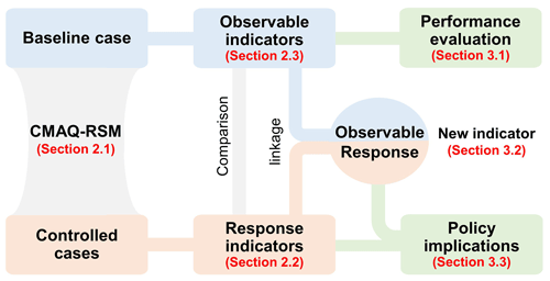
The design of an effective O3 and PM2.5 control strategy requires efficient quantification of air pollutant sensitivity to precursor emissions. Indicator studies have demonstrated that the nonlinear response of O3 and PM2.5 to precursors can be estimated by using ambient concentrations of related chemical species. It is expected that the response indicators originally derived from RSM predictions (i.e., PR and FR) can also be calculated using a combination of ambient concentrations of certain chemical species, enabling these indicators to become observable indicators rather than being dependent on numerous CTM simulations. To support the needs of policy design for O3 and PM2.5 control, this study developed effective indicators that not only represent O3 and PM2.5 chemistry but also aid in determining the most feasible emission reduction path, similar to the benefits provided by RSM-based indicators. The flow of this study is presented in Fig. 1. The new observable response indicators were developed by investigating the link between observable and RSM-based indicators in China.
The remainder of this paper is structured as follows: Sect. 2 presents the detailed methods for CTM modeling, RSM configuration and response indicator development. Section 3 presents the evaluation of the performance of observable indicators in predicting the chemistry regime and the development of the observable response indicators and discusses their policy implications. Section 4 summarizes the main conclusions of this study.
2.1 Configuration of the CTM and RSM
In this study, the Community Multi-scale Air Quality (CMAQ) model (version 5.2) was used to simulate the baseline concentrations of O3 and PM2.5 and their responses in numerous emission control scenarios with different emission change ratios. The simulation was conducted on a domain covering China with 27 km × 27 km horizontal resolution (Fig. 2). In 2017, January, April, July, and October were simulated to represent winter, spring, summer, and fall, respectively. An annual level was estimated as the average of the levels in these four months. The concentration data were analyzed based on the monthly average for afternoon O3 (12:00–18:00 China standard time when O3 was the highest across a day) and monthly average for 24 h PM2.5. To approximate exposure concentrations, we also estimated population-weighted O3 and PM2.5 at the regional or national level by averaging the gridded concentrations weighted by the population in each grid cell. The gridded population data were obtained from the 1 km × 1 km LandScan population dataset in 2016 (Oak Ridge National Laboratory, 2013).
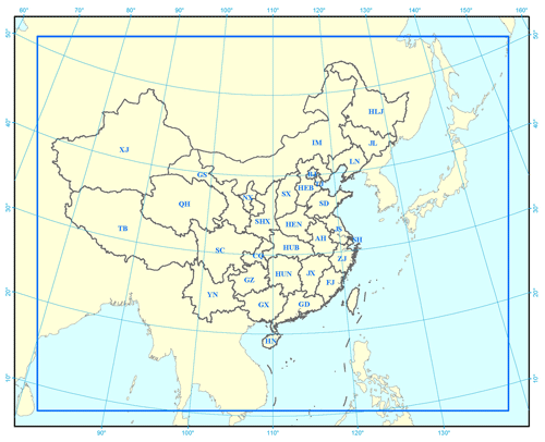
Figure 2Simulation domain over mainland China (27 km × 27 km resolution, 182×232 grid cells). The 31 provinces are BJ – Beijing; TJ – Tianjin; HEB – Hebei; SX – Shanxi; IM – Inner Mongolia; LN – Liaoning; JL – Jilin; HLJ – Helongjiang; SH – Shanghai; JS – Jiangsu; ZJ – Zhejiang; AH – Anhui; FJ – Fujian; JX – Jiangxi; SD – Shandong; HEN – Henan; HUB – Hubei; HUN – Hunan; GD – Guangdong; GX – Guangxi; HN – Hainan; CQ – Chongqing; SC – Sichuan; GZ – Guizhou; YN – Yunnan; TB – Tibet; SHX – Shaanxi; GS – Gansu; QH – Qinghai; NX – Ningxia; and XJ – Xinjiang).
The anthropogenic emission data were developed by Tsinghua University using a bottom-up method (Ding et al., 2019a) with updated activity data from the 2017 China statistical yearbook as well as the latest application rates of end-of-pipe control technologies based on the governmental bulletin and reports. The anthropogenic emissions were gridded into 27 km × 27 km horizontal resolution to match the CMAQ model (Fig. S1). The 2017 biogenic emissions over China were generated using the Model for Emissions of Gases and Aerosols from Nature (MEGAN version 2.04). The meteorology field, driven by the Weather Research and Forecasting Model (WRF version 3.7), followed the same configuration as that in our previous study (Ding et al., 2019a, b) and thus included the Morrison double-moment microphysics scheme, the RRTMG radiation scheme, Kain–Fritsch cumulus cloud parameterization, the Pleim-Xiu land-surface physics scheme and the ACM2 planetary boundary layer (PBL) physics scheme. We used NCEP FNL (Final) Operational Global Analysis data for the initial and boundary conditions in the WRF. The comparison with observation data from the National Climatic Data Center suggested agreeable performance of the WRF model for simulating wind speed, humidity and temperature (Table S1). The CMAQ model performance in reproducing O3 and PM2.5 concentrations was evaluated by comparison with the ground-based observations (Fig. S2), which suggested acceptable CMAQ model performance that met the recommended benchmark (Ding et al., 2019a, b). The normalized mean biases of CMAQ in predicting PM2.5 and O3 are −16.4 % and −12.5 % compared with monitoring data obtained from the China National Environmental Monitoring Centre. The mean fractional biases for PM2.5 and O3 prediction are −14.2 % and −11.1 %, respectively (within the benchmark of ±60 %). The mean fractional errors for PM2.5 and O3 prediction are 21.6 % and 17.0 %, respectively (within the benchmark of 75 %). The RSM was developed based on multiple CTM simulations for various emission-control scenarios according to the brute-force method. Identical to our previous RSM studies (Xing et al., 2017, 2018), the responses of O3 and PM2.5 to precursor emissions were analyzed using the baseline case and 40 control scenarios using the Latin hypercube sample method for four control variables, namely the emission ratios of NOx, SO2, NH3 and VOCs. Though the responses of O3 and PM2.5 to local or regional emissions vary significantly as suggested in our previous study (Xing et al., 2011), we applied the same change ratio of each pollutant emission to all regions across China in this study. This approach is consistent with the implementation of a multiregional joint control strategy, which is reasonable for China. The same level of local and regional emission reduction has been recommended to achieve China's aggressive air quality goals (Xing et al., 2019).
The control matrix is provided in Table S2. The range of emission changes is set as 0 to 2 to be consistent with our previous studies in which the pf-RSM performance has been well examined (Xing et al., 2011, 2018; Wang et al., 2011; Ding et al., 2019b). The pf-RSM performance in predicting PM2.5 and O3 responses has been evaluated in detail using leave-one-out cross validation as well as the out-of-sample validation method, with normalized errors all within 5 % for both PM2.5 and O3 across the domain. Relatively large biases occurred for marginal cases, where emissions are controlled by nearly 100 % and predicted concentrations are very small. These cases have limited influence on the shape of the nonlinear curve of the response function. However, the RSM is developed from a suite of CMAQ simulations, and so uncertainties in the chemical mechanism used in CMAQ might influence the O3 and PM2.5 predictions.
2.2 RSM-based indicators of O3 and PM2.5 chemistry
Based on the developed pf-RSM, the nonlinear responses of O3 and PM2.5 concentrations to precursor emissions can be represented as follows:
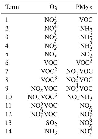
where ΔConc is the change in O3 or PM2.5 concentration from the baseline concentration calculated from a polynomial function of four variables (, , , ΔEVOCs); , , , and ΔEVOCs are the change ratios of NOx, SO2, NH3, and VOC emissions (i.e., ΔEmissions/Baseline_Emissions), respectively, relative to the baseline emissions (baseline = 0); and ai, bi, ci, and di are the nonnegative integer powers of , , , and ΔEVOCs, respectively. Xi is the coefficient of term i for the 14 (n) terms listed in Table 1.
The terms used to represent PM2.5 and O3 responses were determined in designing the pf-RSM (Table 1). The high-degree terms of NOx, VOCs and NH3 represent their strong nonlinear contributions to O3 or PM2.5. The interaction terms of NOx and VOC for PM2.5 and O3 represent the nonlinearity in atmospheric oxidations, whereas those of NOx and NH3 for PM2.5 represent aerosol thermodynamics (Xing et al., 2018).
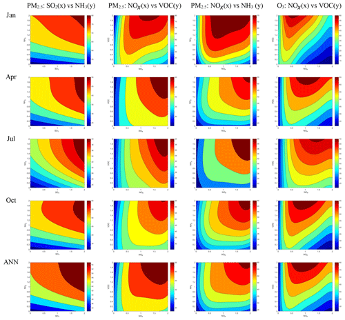
Figure 3Isopleth of population-weighted PM2.5 and daytime O3 to precursor emission change in different months. (The x and y axes represent precursor emission rates with a baseline of 1, applied to all grid cells in China; background colors represent the population-weighted PM2.5 and daytime O3 concentrations in China, with units of micrograms per cubic meter for PM2.5 and parts per billion for O3.)
Xi was fitted by 40 CTM control scenarios for each spatial grid cell. The Xi values in the pf-RSM for annual-averaged population-weighted O3 and PM2.5 concentrations in 31 provinces in China are provided in Tables S3 and S4, respectively. The terms with the first degree for NOx, SO2, NH3, and VOCs represent the first derivative of PM2.5 and O3 response to each precursor emission. O3 was more sensitive to NOx (term X5) and VOCs (term X6) than to SO2 (term X13) or NH3 (term X14), and O3 sensitivity was negative to NOx but positive to VOCs in most provinces. PM2.5 sensitivities to the four precursors (terms X1, X2, X5, and X11 for VOCs, NH3, SO2, and NOx, respectively) were comparable, whereas PM2.5 sensitivity to NOx could be negative or positive.
The nonlinearities of O3 and PM2.5 to precursors were mainly determined by high-order and interaction terms. To illustrate such nonlinearities further, we used a series of isopleths, as shown in Fig. 3, as an example to present the national-averaged PM2.5 response to SO2 and NH3 and NOx and NH3 as well as PM2.5 and O3 responses to NOx and VOCs in different months. Strong nonlinearity was noted in PM2.5 sensitivity to NH3 and in O3 and PM2.5 sensitivities to NOx. PM2.5 sensitivity to NH3 increased alongside the transition of PM2.5 chemistry from the NH3-rich condition (typically at high NH3 emission ratios) to the NH3-poor condition (typically at low NH3 emission ratios). O3 and PM2.5 sensitivities to NOx were negative under the NOx-saturated regime (typically at high NOx emission ratios) but became positive under the NOx-limited regime (typically at low NOx emission ratios). In addition, the transition points (corresponding to the NOx or NH3 ratios at which the chemical regime for O3 or PM2.5 chemistry changed) varied by time (Fig. 3) and space (see the isopleths at different provinces in Figs. S3–S6). In general, the NH3-poor condition appears in winter because of low NH3 evaporation and little agriculture activity, which is a dominant NH3 source. The strong NOx-saturated condition appears in winter when photolysis is less active than in other seasons and concentrates in industrial regions with abundant NOx emissions.
Table 2Summary of observable indicators and their performances in predicting O3 chemistry.

∗ TV – transition value as summarized in Zhang et al. (2009); TV' – transition value proposed in this study.
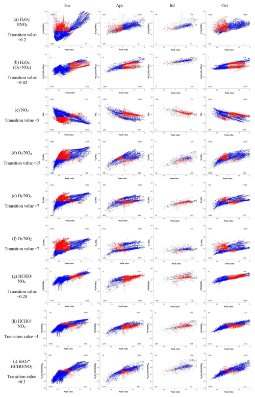
Figure 4Performance of observable indicators in predicting O3 chemistry. The x axis represents the PR values where the transition value is 1, and the y axis represents the observable indicators. The blue dots represent the grids where O3 chemistry is successfully predicted by the observable indicator; the red dots represent the grids where the observable indicator fails to predict O3 chemistry. The numbers in the four corners represent the grid number in each section; the number in July is much lower than those in the other months because most grids are located at the NOx-limited regime with PR>2 in July.
ΔC_NH3 (the unit is micrograms per cubic meter of PM2.5 per 10 % NH3 reduction) can be calculated as follows:
Table 3Summary of observable indicators and their performances in predicting PM2.5 chemistry.

∗ TV – transition value as proposed in Zhang et al. (2009); TV – transition value as proposed in this study.
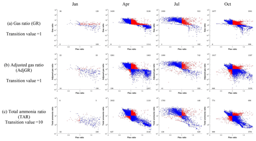
Figure 5Performance of observable indicators in predicting PM2.5 chemistry. The x axis represents the FR values where the transition value is 1, and the y axis represents the observable indicators. The blue dots represent the grids where PM2.5 chemistry is successfully predicted by the observable indicator; the red dots represent the grids where the observable indicator fails to predict PM2.5 chemistry. The numbers in the four corners represent the grid number in each section; the number in January is much lower than those in the other months because most grids are located in the NH3-poor conditions with FR>2 in January.
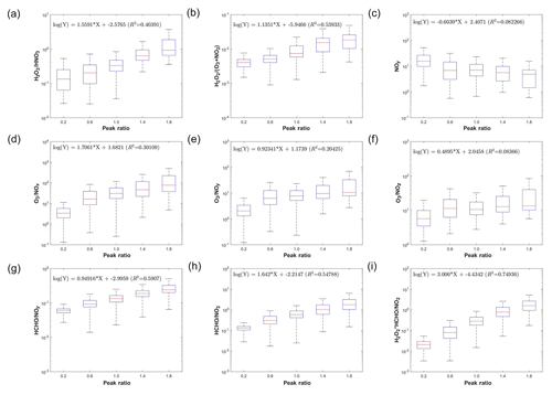
Figure 6Development of observable responsive indicators for O3 chemistry based on log-linear regressions between observable indicators and the PR.
To further quantify the aforementioned nonlinearity, two RSM-based response indicators (i.e., the PR for O3 and FR for PM2.5) were calculated as described in our previous studies (Xing et al., 2011, 2018; Wang et al., 2011).
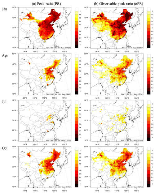
Figure 7Comparison of the PR derived from the RSM with that calculated from concentrations for O3 chemistry. The oPR was estimated based on H2O2 × HCHO∕NO2.
For O3, the PR can be directly calculated as follows:
where is the first derivative of the to , which can be derived as follows:
The PR is the NOx emissions (represented as ) that produce maximum O3 concentration under the baseline VOC emissions. For PR<1, the baseline condition is NOx saturated, and the level of simultaneous control of VOCs to prevent an increase in O3 levels from the NOx controls must be understood. This level is defined by the ratio of VOCs to NOx (i.e., VNr) corresponding to the PR and is calculated as follows:
where is the first derivative of the to . When , and and are 0, can be written as follows:
Since the is close to 0 when the controls are taken from the baseline, we ignore the terms of in the first derivative function above, and then it can be written as follows,
The VNr therefore can be calculated using the following equation:
For PM2.5, the FR can be directly calculated from the polynomial function of PM2.5 by estimating the second derivative of the PM2.5 response to NH3 emissions without considering interaction with other pollutants (Xing et al., 2018). In this study, we selected a simplified method to calculate the FR, estimated as the corresponding NH3 emission ratio when the PM2.5 sensitivity to NH3 and NOx emissions is equal under the baseline conditions (similar to the definition in Wang et al., 2011, but here we calculated the sensitivity of PM2.5 instead of nitrate in this study):
where and are the first derivatives of the ΔConcPM to and , respectively, and can be obtained as follows:
The FR is the NH3 emissions (represented as that correspond to the inflection point between NH3-rich and NH3-poor conditions under baseline NOx emissions. A FR greater than 1 indicates that the baseline condition is NH3 poor, and a FR less than 1 indicates that the baseline condition is NH3 rich. The extra benefit in PM2.5 reduction (denoted as ΔC_NH3) from simultaneous NH3 controls in the same percentage as the required NOx controls can be quantified as follows:
where is the first derivative of the response to when , and
is the first derivative of the response to when .
2.3 Observable indicators of O3 and PM2.5 chemistry
Zhang et al. (2009) summarized the various observable indicators with their corresponding transition values to identify O3 and PM2.5 chemistry: O3 indicators were H2O2∕HNO3, , NOy, O3/NOx, O3/NOy, O3∕NOz, HCHO/NOy, and HCHO/NO2, and the PM2.5 indicators were the DSN, GR, and AdjGR (defined in Text S1); these indicators have been used extensively in previous research (Liu et al., 2010; Wang et al., 2011; Ye et al., 2016). In the current study, we evaluated all the aforementioned indicators except DSN (DSN is included in the definition of the AdjGR; thus it was not considered as a separate indicator in this study). The original transition values, summarized by Zhang et al. (2009), are listed in Table 2. In the present study, we examined these transition values and compared their performance in predicting O3 and PM2.5 chemistry. Because the RSM-based indicators, PR and FR, are calculated using the multiple CTM simulations that use state-of-the-science representations of O3 and PM2.5 chemistry, these indicators were assumed to represent the true condition for comparison with the condition predicted using observable indicators. The performance of each observable indicator is described by its success rate, which is the ratio of the number of correct predictions to the total number of predictions. A correct prediction is indicated by the observable indicator providing consistent results for O3 or PM2.5 chemistry as suggested by PR or FR. The comparison is only conducted for spatial grid cells with valid PR or FR values within the range of 0 (fully controlled emissions) to 2 (double emissions).
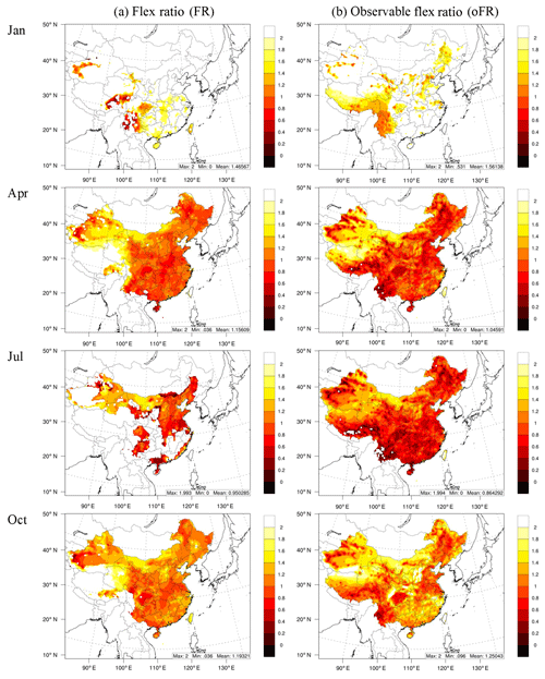
Figure 9Comparison of the FR derived from the RSM with that calculated from concentrations for PM2.5 chemistry. The oPR was estimated based on TAR.
As RSM-based indicators, the PR and FR have meaningful values that can be used to illustrate the extent of the chemistry regime. The linkage of observable indicators with the PR and FR was investigated by performing a linear-log regression of the value of the original observable indicator and the values of the PR or FR as follows:
where Y is an observable indicator for O3 or PM2.5, X is the RSM-based indicator (i.e., PR for O3 or FR for PM2.5), and the coefficients A and B are estimated based on statistical regression. Therefore, the observable response indicators (X′) can be calculated as follows:
The observable response indicators have the same policy implication as that of PR or FR, but they can be directly calculated from the baseline concentrations of certain chemical species rather than being derived from multiple CTM simulations. Therefore, these indicators are considerably more efficient than traditional RSM-based indicators.
3.1 Evaluating observable indicator performance in predicting chemistry regimes
3.1.1 O3
Observable indicators and the PR are compared in Fig. 4, and the performance of observable indicators in predicting O3 chemistry is summarized in Table 2. In general, strong correlation was noted between the observable indicators and PR. The indicator with the highest annual success rate was H2O2∕HNO3 at approximately 73.4 %, with a value of 0.2 for the transition from NOx-saturated to NOx-limited conditions. However, the original transition value of 0.2 for H2O2∕HNO3 tended to be too low, particularly in April, July and October (see Fig. 4a). This study found that the annual success rate of H2O2∕HNO3 could be increased to 80.5 % if 0.3 was used as the transition value. This finding was consistent with corresponding findings in previous studies, which have suggested the transition values of H2O2∕HNO3 to be within the range of 0.2–3.6 at different locations and in different seasons (Sillman, 1995; Sillman et al., 1997; Lu and Chang, 1998; Tonnesen and Dennis, 2000; Hammer et al., 2002; Liang et al., 2006; Zhang et al., 2009). , with a transition value of 0.02, also exhibited a high annual success rate of 66.4 %; this rate could be increased to 71.1 % by applying a transition value of 0.005 because the original transition value was too high, particularly in January, April and October (see Fig. 4b). HCHO∕NOy and HCHO∕NO2 exhibited relatively low performance, particularly in April and July, because the original transition values appeared to be too high (Fig. 4g and h). However, the performance of HCHO∕NOy and HCHO∕NO2 could be greatly improved by using lower transition values, with increased annual success rates as high as 76 %. The change of the transition values implies that such indicators cannot fully consider all factors that determine the O3 chemistry by using concentrations of just two species. The transition values of the indicators NOy, O3∕NOx, O3∕NOy and O3∕NOz were suitable for estimating annual levels if only one unique transition value was applied for all months (apparently, these transition values for O3∕NOx, O3∕NOy and O3∕NOz in January and NOx in April and July may have been too low). However, their success rates (all <70 %) were not as high as those of other indicators. The inferior performance of the three O3-involved indicators (O3∕NOx, O3∕NOy and O3∕NOz) may have been associated with the considerable effects of background O3, which cannot be removed easily.
Because and HCHO∕NO2 exhibited good performance in predicting O3 chemistry, this study proposed a new indicator combining these two indicators, namely H2O2 × HCHO∕NO2, with a transition value of 0.3. The results suggested that this new indicator has the highest annual success rate, namely 87.3 %, among all the indicators. Studies (Sillman, 1995; Tonnesen and Dennis, 2000) have suggested that HCHO is approximately proportional to the VOC reactivity (i.e., the weighted sum of the reactions of VOCs with OH) and that HCHO∕NO2 closely approximates the competition between OH reactions with VOC and NO2 that is central to O3 chemistry. H2O2 derives from a key radical termination pathway under low-NOx conditions (HO2+HO2 → H2O2+O2). Comparison of H2O2 with NOy or HNO3, which derives from a key radical termination pathway under high-NOx conditions (OH + NO2 → HNO3), represents the relative abundance of VOCs to NOx. The new hybrid indicator incorporates information from the two individual indicators and could potentially be more robust.
3.1.2 PM2.5
We selected the GR and AdjGR as observable indicators for PM2.5 chemistry to identify NH3-poor or NH3-rich conditions. Comparison of GR and AdjGR with the FR is detailed in Fig. 5. AdjGR performance was much higher than that of the GR, with a larger annual success rate of 74.1 % compared with the GR's 55.6 % (see Table 3). The transition value of the GR appeared to be too low in all months (Fig. 5a). This result was consistent with those of previous studies; the AdjGR tends to be a more robust indicator because in contrast to the GR, it does not require an assumption of full sulfate neutralization (Zhang et al., 2009). The improvement of AdjGR compared to GR is the greatest in January and the smallest in July (Table 3). This is consistent with Pinder et al. (2008), who showed that accounting for DSN is important under cold temperatures, but GR and AdjGR converge for higher temperatures.
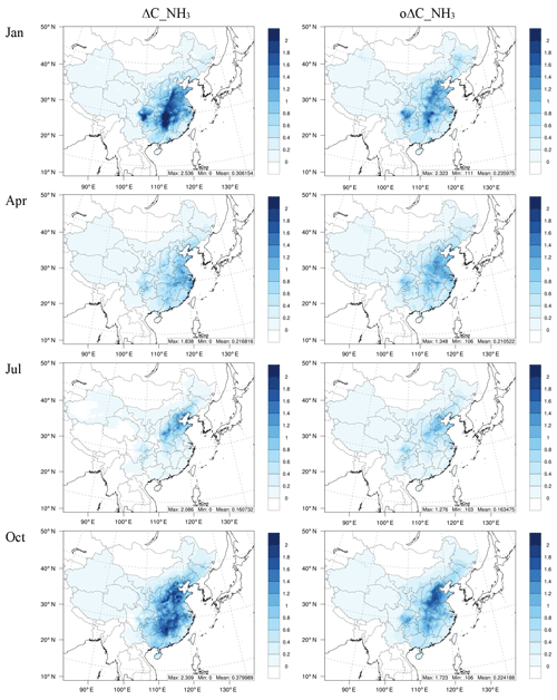
Figure 12Comparison of the benefit in reducing PM2.5 from simultaneous NH3 reduction (ΔC_NH3) with that calculated from concentrations (oΔC_NH3).
This study designed a new indicator, total ammonia ratio (TAR), where the sulfate concentration is involved in the calculation, as follows:
where [TN] and [TS] are the total molar concentrations of nitrate and sulfate , respectively, and TAR is the relative abundance of total ammonia to nitrate and sulfate, regarded as the product of [TA]∕[TN] and [TA]∕[TS]. To simplify the calculation, [TA]2 is assumed to be the product of the molar concentration of ammonia gas [NH3] and ammonium [].
The performance of TAR in predicting PM2.5 chemistry was slightly higher than that of AdjGR, as demonstrated by the higher success rate of TAR than that of AdjGR in all months. The annual success rate of TAR was 79.6 %, with a transition value of 10 (Table 3).
3.2 Developing the observable responsive indicators
3.2.1 O3
Figure 6 presents the log-linear regressions of the O3 observable indicators on the PR indicator derived from the RSM. In general, all observable indicators exhibited strong correlations with the PR (all except NOy presented positive correlations with the PR), with varying R2 values (0.08–0.75). The indicators including NOy, O3∕NOx, O3∕NOy and O3∕NOz, which had relatively low success rates, exhibited weaker correlation with the PR (R2<0.31; Fig. 6c–f). The newly developed H2O2 × HCHO∕NO2 indicator exhibited the strongest correlation with the PR (R2=0.75), implying that the log-linear combination of the H2O2, HCHO and NO2 baseline concentrations could approximate the responsive PR indicator to quantify O3 chemistry. Other indicators can also be used to approximately estimate the PR based on the regression coefficients shown in Fig. 6; however, their correlations with the PR were not as strong as those with H2O2 × HCHO∕NO2.
To evaluate the ability of the observable PR (oPR; estimated based on H2O2 × HCHO∕NO2) to represent the spatial and temporal variation in O3 chemistry, the spatial distribution of the PR and oPR in the four study months was compared across the simulated domain (Fig. 7). The oPR successfully captured the strong NOx-saturated regime in January (PR<1) and the NOx-limited (PR>1) regime in July.
In addition, the PR and oPR suggested a consistently strong NOx-saturated regime in northern and eastern China and key regions such as the YRD and PRD. The domain-averaged oPRs were 0.97, 1.52, 1.73, and 1.37 in January, April, July, and October, respectively; these values are similar to the PRs (0.77, 1.24, 1.38 and 1.17, respectively). Thus, the oPR may approximate the PR to quantify the O3 chemistry, even on a large spatial and temporal scale.
3.2.2 PM2.5
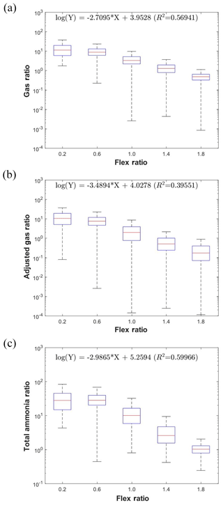
The correlations between PM2.5 observable indicators and the responsive FR indicator derived from the RSM were investigated (Fig. 8). The AdjGR has the lowest R2 (0.40) because of its high variations for the NH3-poor condition (Fig. 5b). A stronger positive correlation was noted between the GR and FR (R2=0.57); however, the success rate of the GR was the lowest among all the indicators (the success rate of the GR increased when the transition value was set as the median value of the GR, namely 5, at an FR of 1). The TAR exhibited the strongest positive correlation with the FR (R2=0.60), implying that the FR can be approximately estimated by the log-linear combination of baseline concentrations of ammonia gas, nitric acid gas, particulate ammonium, sulfate and nitrate.
The capability of the observable FR (oFR; estimated based on the TAR indicator) in representing the spatial and temporal variation in PM2.5 chemistry is illustrated in Fig. 9. Both the FR and oFR suggested strong NH3-poor conditions (FR>1) in January and NH3-rich conditions (FR<1) in April and July. The oFR suggested strong NH3-rich conditions in northern and eastern China and the Sichuan Basin; these findings were consistent with those for the FR. The domain-averaged oFRs were 1.56, 1.05, 0.86, and 1.24 in January, April, July, and October, respectively, with the strongest NH3-poor conditions in January and NH3-rich conditions in July. These findings were comparable with the FRs of 1.47, 1.16, 0.95 and 1.19 for the four study months, respectively, suggesting that the oFR can approximate the FR to quantify the PM2.5 chemistry and its spatial and temporal variations.
3.3 Policy implications
3.3.1 O3
The responsive PR indicator may help policy-makers to understand the status and extent of O3 chemistry in the current scenarios. A lower PR (<1) suggested a NOx-saturated regime. Moreover, the VNr could be used to inform policy-makers about the level of simultaneous control of VOCs required to prevent an increase in O3 levels from NOx controls. In general, the VNr is negatively correlated with the PR because a lower PR implies a stronger NOx-saturated regime, which in turn requires more simultaneous VOC control with NOx. By contrast, a higher PR implies a weaker NOx-saturated or even NOx-limited regime, which requires less or no simultaneous control of VOCs with NOx. The negative correlation between VNr and the PR was quantified by the simple linear regression of VNr on PR (Fig. S7). A high R2 (approximately 0.82) suggested that the VNr originally derived from the RSM can also be approximately estimated from the PR or oPR.
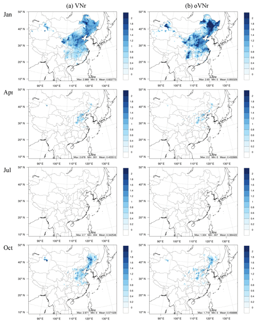
Figure 10 presents a comparison of the VNr derived from the RSM, with the VNr calculated based on the oPR, estimated by the H2O2 × HCHO∕NO2 indicator and denoted as oVNr. Consistent spatial and temporal variations were found for VNr and oVNr. Additional simultaneous VOC control is required in January and in northern and eastern China and is highly correlated with the low PR (Fig. 7). The domain-averaged oVNr values were estimated to be 0.95, 0.43, 0.38, and 0.47 in January, April, July, and October, respectively, with the highest and lowest oVNr values noted in January and July, respectively. This is comparable with VNr in the four study months (i.e., 0.82, 0.46, 0.34, and 0.57, respectively).
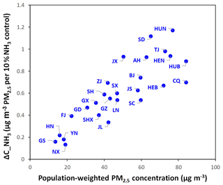
Figure 13Comparison of annually averaged benefit in reducing PM2.5 from simultaneous NH3 reduction (ΔC_NH3) and population-weighted PM2.5 concentration in each province in China.
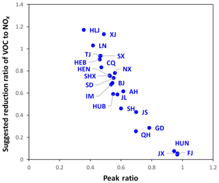
The annually averaged VNr and PR were also calculated for each province in China (Fig. 11). VNr was negatively correlated with the PR at the provincial level. The northern provinces, namely Heilongjiang, Xinjiang, and Liaoning, required the highest VNr (1–1.2) because their PRs were very low (0.3–0.4). In the NCP, including the provinces of Tianjin, Hebei, Henan, Shandong, Shanxi, Inner Mongolia and Beijing, high VNr (0.7–0.9) was required to overcome the stronger NOx-saturated regime (PR=0.4–0.6). The coastal provinces, namely Fujian and Guangdong, and middle-eastern provinces, namely Jiangxi and Hunan, also demonstrated relatively high PRs (>0.7) and low VNr (<0.3).
3.3.2 PM2.5
Using the responsive FR indicator or its observable oFR indicator can rapidly identify NH3-rich or NH3-poor conditions, and this information can aid policy-makers in estimating the additional PM2.5 benefit associated with simultaneous control of NH3 and NOx emissions (ΔC_NH3). As discussed in Sect. 2.2, ΔC_NH3 can be calculated from the RSM using the first derivative of the PM2.5 responsive function to NH3. Therefore, ΔC_NH3 must be strongly associated with the secondary inorganic aerosol (SNA) concentration, as suggested in Fig. S8, which demonstrates a strong correlation between SNA concentration and ΔC_NH3. The linear regression with high R2 (>0.71) implies that the ΔC_NH3 can be approximately calculated based on the SNA concentration.
The ΔC_NH3 estimated based on the SNA concentration (oΔC_NH3; based on the regression function in Fig. S8) was compared with that derived from the RSM (Fig. 12). The oΔC_NH3 typically captured the spatial and temporal variation in ΔC_NH3, suggesting large benefits in January and October, particularly in eastern China and the Sichuan Basin. The domain-averaged ΔC_NH3 values were approximately 0.31, 0.22, 0.16, and 0.38 µg m−3 PM2.5 per 10 % NH3 reduction in January, April, July, and October, respectively. In April and July, oΔC_NH3 presented consistent results of approximately 0.21 and 0.16 µg m−3 PM2.5, respectively, per 10 % NH3 reduction, but slightly underestimated the benefits in January and October (0.24 and 0.22 µg m−3 PM2.5, respectively, per 10 % NH3 reduction).
At the annual level, ΔC_NH3 was compared with the population-weighted PM2.5 concentration in each province (Fig. 13). ΔC_NH3 ranged from 0.2 to 1.2 µg m−3 PM2.5 per 10 % NH3 reduction. In addition, the provinces with higher PM2.5 exposure exhibited additional benefits from NH3 reductions (i.e., high ΔC_NH3), particularly in Hunan, Shandong, Tianjin, Jiangxi, Anhui, Henan and Hubei where ΔC_NH3 was >0.8 µg m−3 PM2.5 per 10 % NH3 reduction. These benefits from simultaneous NH3 control were substantial enough to be considered in these regions for achieving the national ambient PM2.5 target (35 µg m−3).
3.3.3 Co-benefits of NOx and VOC control in reducing O3 and PM2.5
NOx and VOCs are major precursors for O3 and PM2.5, and effectively controlling their emissions can lead to co-benefits in reducing O3 and PM2.5. The PR results suggest strong NOx-saturated regimes in northern and eastern China including key regions such as the Sichuan Basin, YRD and PRD, where simultaneous VOC control with a certain VOC-to-NOx ratio is required to prevent increases in O3 levels from the NOx controls. PM2.5 sensitivity to NOx can be negative under a strong NOx-saturated regime; this effect is not as significant as it is for O3 (Fig. 3). We quantified the nonlinearity of PM2.5 sensitivity to NOx by using the same PR concept but for PM2.5 response (Sect. S2); Fig. S9 presents the spatial distribution of the PR to identify PM2.5 sensitivity to NOx emission in the four study months. The PR values for PM2.5 were >1 in April, July and October in all grid cells across China, suggesting that NOx control is always beneficial for PM2.5 reduction during these months. Even in January, the PR for PM2.5 (0.4–0.8 in eastern and northern China) remains larger than that for O3 (0.2–0.6 in eastern and northern China), implying that the suggested VNr for O3 was high enough to overcome the potential limitations on PM2.5 reduction from NOx control.
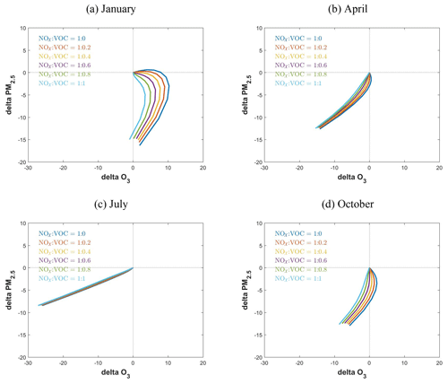
To explore the co-benefits of reducing O3 and PM2.5 after simultaneous control of NOx and VOCs, we investigated the effectiveness of six control pathways with various VOC-to-NOx ratios including 0, 0.2, 0.4, 0.6, 0.8 and 1.0 (Fig. 14). In general, O3 and PM2.5 concentrations can be reduced in all months through simultaneous control of NOx and VOC emissions, although different VNr and control levels are required in different months. In January (under strongly NOx-saturated conditions), reductions in PM2.5 and O3 require VOC emission controls in addition to NOx controls to prevent potential disbenefits associated with the nonlinear chemistry. The smaller VNr required for PM2.5 (∼0.4) than for O3 (∼1.0) in this case might be associated with the smaller PR for PM2.5 as well as the additional benefit of VOC controls in reducing secondary organic aerosols. Apparently, a larger VNr control ratio and greater emission control is required in January compared with other months. In Fig. 14a, only one pathway can achieve simultaneous reduction in O3 and PM2.5 concentrations (i.e., the pathway with VNr equal to 1 and at the far end of the pathway, with reduction rates >80 %). In April and October, simultaneous VOC controls were still required for O3 (VNr = 0.2–0.6) but not for PM2.5. In July when the NOx-limited regime was dominant, the NOx control was critical because the VOC controls had little effect on either O3 or PM2.5. At the annual level, the simultaneous VOC controls (40 % of the NOx controls) led to co-benefits in reducing both O3 and PM2.5 at the national level. However, VNr varied significantly in different seasons, suggesting that considering the seasonality of O3 and PM2.5 chemistry is necessary for design of a season-specific control strategy.
Compared with conducting multiple CTM simulations, the indicator method proved more efficient in identifying the chemical regime in the current scenarios. However, the traditional indicators are not as useful as the RSM-based PR and FR indicators for policy-makers to infer feasible emission reduction paths. Therefore, this study quantified the relationship between RSM-based and traditionally observable indicators and developed new observable response indicators, the oPR and oFR, which can be used to quantify the nonlinearity of O3 and PM2.5 response to precursor emissions. Similar to the traditional indicators, the oPR and oFR can be easily calculated using a combination of ambient concentrations of certain chemical species obtained from surface-monitored observations, modeling simulations or even satellite retrievals. In addition, the observable responsive indicators can not only rapidly identify the chemical regime but also provide policy-makers with useful information, such as simultaneous VOC controls to prevent increases in O3 levels from NOx controls under the NOx-saturated regime (i.e., VNr), as well as the additional benefit of simultaneously reducing NH3 alongside NOx control in PM2.5 reductions (i.e., ΔC_NH3). Since the indicators are developed from simulations with spatially uniform emission controls across the country, they are especially useful for providing quick estimates of the potential benefits or risks from uniform controls. These estimates can also provide a basis to design more localized control strategies for particular regions.
This study proposed a new O3 chemistry indicator, namely H2O2 × HCHO∕NO2, and PM2.5 chemistry indicator, namely the TAR, both of which exhibited the highest success rates among all the indicators. This study also suggested that the log-linear combinations of baseline H2O2, HCHO and NO2 concentrations could provide an approximate PR to quantify O3 chemistry spatially and temporally. Similarly, the log-linear combination of baseline concentrations of ammonia gas, nitric acid gas, particulate ammonium, sulfate and nitrate can be used to approximately estimate the FR for PM2.5 chemistry. The VNr was highly correlated with the PR, suggesting that a stronger NOx-saturated regime requires greater VOC control accompanied by NOx control. The positive correlation between ΔC_NH3 and the population-weighted PM2.5 concentration suggested that a province with high PM2.5 exposure can gain greater benefits from NH3 reduction. Finally, simultaneous control of NOx and VOC could reduce both O3 and PM2.5 throughout the year, and an effective control pathway (VNr = 0.4) could lead to the co-benefits of reducing both O3 and PM2.5. However, VNr varied significantly among the seasons and provinces, suggesting the necessity of considering the seasonality of chemistry and of designing a more localized control strategy for each province. We note that the discrepancy between the observable indicator and the responsive indicator might also be influenced by uncertainties in the chemical mechanism of CMAQ as well as prediction errors of the pf-RSM. The new indicators were designed based on the existing chemical mechanism, and the transition values might be refined in the future as our understanding of atmospheric chemical processes improves.
In conclusion, the two unique aspects of this study are as follows. First, quantification of the correlation of observable indicators with responsive indicators (Figs. 5 and 7) implied that the traditional observable indicators, based on monitored or satellite-retrieved concentrations, can be used to quantify the nonlinearity of PM2.5 and O3 to precursor emission and provide useful policy implications. Second, this study reported a promising method for efficiently establishing PM2.5- and O3- responsive functions to precursors for traditional responsive or reduced-form modeling studies. This study suggested that the PR or FR (a combination of coefficients in the polynomial functions in the pf-RSM) can be approximately estimated using the ambient concentration of certain chemical species. Similarly, all coefficients in polynomial functions can be calculated based on a set of ambient concentrations of certain chemical species. The simple log-linear regression method used in this study demonstrated the possibility that even in the presence of uncertainties in prediction, more advanced data analytics technologies such as deep learning may improve performance in future.
The pf-RSM outputs and code package are available from the corresponding author upon request.
The supplement related to this article is available online at: https://doi.org/10.5194/acp-19-13627-2019-supplement.
JX and DD contributed equally to this work. JX designed the methodology and wrote the paper. DD conducted the modeling experiment and analyzed the data. SW provided ideas and financial support and edited the paper. ZD and YZ helped with the modeling experiment. JK, CJ and JH provided ideas and edited the paper.
Although this work was reviewed by the U.S. EPA and approved for publication, the views in the article are those of the authors alone and do not necessarily reflect the policy of the agency. Mention of commercial products does not constitute endorsement by the agency.
This work was completed on the “Explorer 100” cluster system of Tsinghua National Laboratory for Information Science and Technology.
This research has been supported by the National Key R & D program of China (grant nos. 2017YFC0210006 & 2018YFC0213805), the National Natural Science Foundation of China (grant nos. 21625701 & 51861135102), Beijing Municipal Science and Technology Project (grant no. Z181100005418018), and the Shanghai Environmental Protection Bureau (grant no. 2016-12).
This paper was edited by Joshua Fu and reviewed by three anonymous referees.
Ansari, A. S. and Pandis, S. N.: Response of inorganic PM to precursor concentrations, Environ. Sci. Technol., 32, 2706–2714, 1998.
Cohan, D. S., Hakami, A., Hu, Y., and Russell, A. G.: Nonlinear response of ozone to emissions: source apportionment and sensitivity analysis, Environ. Sci. Technol., 39, 6739–6748, 2005.
Cohen, A. J., Brauer, M., Burnett, R., Anderson, H. R., Frostad, J., Estep, K., Balakrishnan, K., Brunekreef, B., Dandona, L., Dandona, R., and Feigin, V.: Estimates and 25-year trends of the global burden of disease attributable to ambient air pollution: an analysis of data from the Global Burden of Diseases Study 2015, The Lancet, 389, 1907–1918, 2017.
Dennis, R. L., Bhave, P. V., and Pinder, R. W.: Observable indicators of the sensitivity of PM2.5 nitrate to emission reductions – Part II: Sensitivity to errors in total ammonia and total nitrate of the CMAQ-predicted non-linear effect of SO2 emission reductions, Atmos. Environ., 42, 1287–1300, 2008.
Ding, D., Xing, J., Wang, S., Liu, K., and Hao, J.: Estimated Contributions of Emissions Controls, Meteorological Factors, Population Growth, and Changes in Baseline Mortality to Reductions in Ambient PM2.5 and PM 2.5-Related Mortality in China, 2013–2017, Environ. health perspectives, 127, 067009, https://doi.org/10.1289/EHP4157, 2019a.
Ding, D., Xing, J., Wang, S., Chang, X., and Hao, J.: Impacts of emissions and meteorological changes on China's ozone pollution in the warm seasons of 2013 and 2017, Front. Environ. Sci. Eng., 13, 76, https://doi.org/10.1007/s11783-019-1160-1, 2019b.
Forouzanfar, M. H., Alexander, L., Anderson, H. R., Bachman, V. F., Biryukov, S., Brauer, M., Burnett, R., Casey, D., Coates, M. M., Cohen, A., and Delwiche, K.: Global, regional, and national comparative risk assessment of 79 behavioural, environmental and occupational, and metabolic risks or clusters of risks in 188 countries, 1990–2013: a systematic analysis for the Global Burden of Disease Study 2013, The Lancet, 386, 2287–2323, 2015.
Freas, W. P., Martinez, E. L., Meyer, E. L., Possiel, N. C., and Sennett, D. H.: Procedures for quantifying relationships between photochemical oxidants and precursors: supporting documentation, EPA-450/2-77-021b, US EPA, Research Triangle Park, North Carolina, 27711, 1978.
Friedlander, S. K.: Smoke, dust and haze: Fundamentals of aerosol behavior. New York, Wiley-Interscience, 333 pp., 1977.
Fuhrer, J., Val Martin, M. , Mills, G., Heald, C. L., Harmens, H., Hayes, F., Sharps, K., Bender, J., and Ashmore, M. R.: Current and future ozone risks to global terrestrial biodiversity and ecosystem processes, Ecol. Evolut., 6, 8785–8799, 2016.
Gipson, G. L., Freas, W. P., Kelly, R. F., and Meyer, E. L.: Guideline for use of city-specific EKMA in preparing ozone SIPs, EPA-450/4-80-027, US Environmental Protection Agency, Research Triangle Park, North Carolina, USA, 1981.
Hakami, A., Odman, M. T., and Russell, A. G.: Nonlinearity in atmospheric response: A direct sensitivity analysis approach, J. Geophys. Res.-Atmos., 109, D15 https://doi.org/10.1029/2003JD004502, 2004.
Hammer, M. U., Vogel, B., and Vogel, H.: Findings on H2O2∕HNO3 as an indicator of ozone sensitivity in Baden-Württemberg, Berlin-Brandenburg, and the Po valley based on numerical simulations, J. Geophys. Res.-Atmos., 107, D22 https://doi.org/10.1029/2000JD000211, 2002.
Jiménez, P. and Baldasano, J. M.: Ozone response to precursor controls in very complex terrains: Use of photochemical indicators to assess sensitivity in the northeastern Iberian Peninsula, J. Geophys. Res.-Atmos., 109, D20, https://doi.org/10.1029/2004JD004985, 2004.
Jin, X., Fiore, A. M., Murray, L. T., Valin, L. C., Lamsal, L. N., Duncan, B., Folkert Boersma, K., De Smedt, I., Abad, G. G., Chance, K., and Tonnesen, G. S.: Evaluating a Space-Based Indicator of Surface Ozone-NOx-VOC Sensitivity Over Midlatitude Source Regions and Application to Decadal Trends, J. Geophys. Res.-Atmos., 122, 19, https://doi.org/10.1002/2017JD026720, 2017.
Li, K., Jacob, D. J., Liao, H., Shen, L., Zhang, Q., and Bates, K. H.: Anthropogenic drivers of 2013–2017 trends in summer surface ozone in China, P. Natl. Acad. Sci. USA, 116, 422–427, 2019.
Liang, J., Jackson, B., and Kaduwela, A.: Evaluation of the ability of indicator species ratios to determine the sensitivity of ozone to reductions in emissions of volatile organic compounds and oxides of nitrogen in northern California, Atmos. Environ., 40, 5156–5166, 2006.
Liu, X. H., Zhang, Y., Xing, J., Zhang, Q., Wang, K., Streets, D. G., Jang, C., Wang, W. X., and Hao, J. M.: Understanding of regional air pollution over China using CMAQ, part II. Process analysis and sensitivity of ozone and particulate matter to precursor emissions, Atmos. Environ., 44, 3719–3727, 2010.
Lu, C. H. and Chang, J. S.: On the indicator-based approach to assess ozone sensitivities and emissions features, J. Geophys. Res.-Atmos., 103, 3453–3462, 1998.
Lu, X., Hong, J., Zhang, L., Cooper, O. R., Schultz, M. G., Xu, X., Wang, T., Gao, M., Zhao, Y., and Zhang, Y.: Severe Surface Ozone Pollution in China: A Global Perspective, Environ. Sci. Technol. Lett., 5, 487–494, https://doi.org/10.1021/acs.estlett.8b00366, 2018.
Megaritis, A. G., Fountoukis, C., Charalampidis, P. E., Pilinis, C., and Pandis, S. N.: Response of fine particulate matter concentrations to changes of emissions and temperature in Europe, Atmos. Chem. Phys., 13, 3423–3443, https://doi.org/10.5194/acp-13-3423-2013, 2013.
Milford, J. B., Gao, D. F., Sillman, S., Blossey, P., and Russell, A. G.: Total reactive nitraogen (NOy) as an indicator of the sensitivity of ozone to reductions in hydrocarbon and NOx emissions, J. Geophys. Res.-Atmos., 99, 3533–3542, https://doi.org/10.1029/93jd03224, 1994.
Myhre, G., Shindell, D., Bréon, F. M., Collins, W., Fuglestvedt, J., Huang, J., Koch, D., Lamarque, J. F., Lee, D., Mendoza, B., and Nakajima, T.: Anthropogenic and Natural Radiative Forcing, in: Climate Change 2013: The Physical Science Basis. Contribution of Working Group I to the Fifth Assessment Report of the Intergovernmental Panel on Climate Change, edited by: Stocker, T. F., Qin, D., Plattner, G.-K., Tignor, M., Allen, S. K., Boschung, J., Nauels, A., Xia, Y., Bex, V., and Midgley, P. M., Cambridge Univ. Press, 2013, 659–740, 2013.
Oak Ridge National Laboratory: Landscan global population dataset 2012, Oak Ridge, Tennessee: Oak Ridge National Laboratory, 2013
Peng, Y. P., Chen, K. S., Lai, C. H., Lu, P. J., and Kao, J. H.: Concentrations of H2O2 and HNO3 and sensitivity in ambient air in southern Taiwan, Atmos. Environ., 40, 6741–6751, 2006.
Pinder, R. W., Dennis, R. L., and Bhave, P. V.: Observable indicators of the sensitivity of PM2. 5 nitrate to emission reductions – Part I: Derivation of the adjusted gas ratio and applicability at regulatory-relevant time scales, Atmos. Environ., 42, 1275–1286, 2008.
Pun, B. K., Seigneur, C., Bailey, E. M., Gautney, L. L., Douglas, S. G., Haney, J. L., and Kumar, N.: Response of atmospheric particulate matter to changes in precursor emissions: a comparison of three air quality models, Environ. Sci. Technol., 42, 831–837, 2007.
Seinfeld, J. H. and Pandis, S. N.: Atmospheric chemistry and physics: from air pollution to climate change, John Wiley & Sons, 2012.
Sillman, S.: The use of NOy, H2O2, and HNO3 as indicators for ozone-NOx-hydrocarbon sensitivity in urban locations, J. Geophys. Res.-Atmos., 100, 14175–14188, 1995.
Sillman, S. and He, D.: Some theoretical results concerning O3-NOx-VOC chemistry and NOx-VOC indicators, J. Geophys. Res., 107, 4659, https://doi.org/10.1029/2001JD001123, 2002.
Sillman, S., He, D., Cardelino, C., and Imhoff, R. E.: The use of photochemical indicators to evaluate ozone-NOx-hydrocarbon sensitivity: Case studies from Atlanta, New York, and Los Angeles, J. Air Waste Manage. Assoc., 47, 1030–1040, 1997.
Sun, Y., Liu, C., Palm, M., Vigouroux, C., Notholt, J., Hu, Q., Jones, N., Wang, W., Su, W., Zhang, W., Shan, C., Tian, Y., Xu, X., De Mazière, M., Zhou, M., and Liu, J.: Ozone seasonal evolution and photochemical production regime in the polluted troposphere in eastern China derived from high-resolution Fourier transform spectrometry (FTS) observations, Atmos. Chem. Phys., 18, 14569–14583, https://doi.org/10.5194/acp-18-14569-2018, 2018.
Takahama, S., Wittig, A. E., Vayenas, D. V., Davidson, C. I., and Pandis, S. N.: Modeling the diurnal variation of nitrate during the Pittsburgh Air Quality Study, J. Geophys. Res.-Atmos., 109, D16, https://doi.org/10.1029/2003JD004149, 2004.
Tonnesen, G. S. and Dennis, R. L.: Analysis of radical propagation efficiency to assess ozone sensitivity to hydrocarbons and NOx: 2. Long-lived species as indicators of ozone concentration sensitivity, J. Geophys. Res.-Atmos., 105, 9227–9241, 2000.
Wang, J., Xing, J., Mathur, R., Pleim, J.E., Wang,, S., Hogrefe, C., Gan, C. M., Wong, D. C., and Hao, J.: Historical trends in PM2.5-related premature mortality during 1990–2010 across the northern hemisphere, Environ. Health Persp., 125, 400 pp , 2017.
Wang, S., Zhao, M., Xing, J., Wu, Y., Zhou, Y., Lei, Y., He, K., Fu, L., and Hao, J.: Quantifying the air pollutants emission reduction during the 2008 Olympic Games in Beijing, Environ. Sci. Technol., 44, 2490–2496, 2010.
Wang, S. X., Xing, J., Jang, C., Zhu, Y., Fu, J. S., and Hao, J.: Impact assessment of ammonia emissions on inorganic aerosols in east China using response surface modeling technique, Environ. Sci. Technol., 45, 9293–9300, 2011.
West, J. J., Ansari, A. S., and Pandis, S. N.: Marginal PM25: nonlinear aerosol mass response to sulfate reductions in the Eastern United States, J. Air Waste Manage. Assoc., 49, 1415–1424, 1999.
Xing, J., Wang, S. X., Jang, C., Zhu, Y., and Hao, J. M.: Nonlinear response of ozone to precursor emission changes in China: a modeling study using response surface methodology, Atmos. Chem. Phys., 11, 5027–5044, https://doi.org/10.5194/acp-11-5027-2011, 2011.
Xing, J., Wang, S., Zhao, B., Wu, W., Ding, D., Jang, C., Zhu, Y., Chang, X., Wang, J., Zhang, F., and Hao, J.: Quantifying Nonlinear Multiregional Contributions to Ozone and Fine Particles Using an Updated Response Surface Modeling Technique, Environ. Sci. Technol., 51, 11788–11798, 2017.
Xing, J., Ding, D., Wang, S., Zhao, B., Jang, C., Wu, W., Zhang, F., Zhu, Y., and Hao, J.: Quantification of the enhanced effectiveness of NOx control from simultaneous reductions of VOC and NH3 for reducing air pollution in the Beijing-Tianjin-Hebei region, China, Atmos. Chem. Phys., 18, 7799–7814, https://doi.org/10.5194/acp-18-7799-2018, 2018.
Xing, J., Zhang, F., Zhou, Y., Wang, S., Ding, D., Jang, C., Zhu, Y., and Hao, J.: Least-cost control strategy optimization for air quality attainment of Beijing–Tianjin–Hebei region in China, J. Environ. Manage., 245, 95–104, 2019.
Ye, L., Wang, X., Fan, S., Chen, W., Chang, M., Zhou, S., Wu, Z., and Fan, Q.: Photochemical indicators of ozone sensitivity: application in the Pearl River Delta, China, Front. Environ. Sci. Eng., 10, p. 15, 2016.
Zhang, Y., Wen, X. Y., Wang, K., Vijayaraghavan, K., and Jacobson, M. Z.: Probing into regional O-3 and particulate matter pollution in the United States: 2. An examination of formation mechanisms through a process analysis technique and sensitivity study, J. Geophys. Res.-Atmos., 114, D22, https://doi.org/10.1029/2009jd011900, 2009.
Zhao, B., Zheng, H., Wang, S., Smith, K.R., Lu, X., Aunan, K., Gu, Y., Wang, Y., Ding, D., Xing, J., and Fu, X.: Change in household fuels dominates the decrease in PM2.5 exposure and premature mortality in China in 2005–2015, P. Natl. Acad. Sci. USA, 115, 12401–12406, 2018.


