the Creative Commons Attribution 4.0 License.
the Creative Commons Attribution 4.0 License.
 | 14 Oct 2019
Impact of synthetic space-borne NO2 observations from the Sentinel-4 and Sentinel-5P missions on tropospheric NO2 analyses
Renske Timmermans
Arjo Segers
Lyana Curier
Rachid Abida
Jean-Luc Attié
Laaziz El Amraoui
Henk Eskes
Johan de Haan
Jukka Kujanpää
William Lahoz
Albert Oude Nijhuis
Samuel Quesada-Ruiz
Philippe Ricaud
Pepijn Veefkind
Martijn Schaap
We present an Observing System Simulation Experiment (OSSE) dedicated to the evaluation of the added value of the Sentinel-4 and Sentinel-5P missions for tropospheric nitrogen dioxide (NO2). Sentinel-4 is a geostationary (GEO) mission covering the European continent, providing observations with high temporal resolution (hourly). Sentinel-5P is a low Earth orbit (LEO) mission providing daily observations with a global coverage. The OSSE experiment has been carefully designed, with separate models for the simulation of observations and for the assimilation experiments and with conservative estimates of the total observation uncertainties. In the experiment we simulate Sentinel-4 and Sentinel-5P tropospheric NO2 columns and surface ozone concentrations at 7 by 7 km resolution over Europe for two 3-month summer and winter periods. The synthetic observations are based on a nature run (NR) from a chemistry transport model (MOCAGE) and error estimates using instrument characteristics. We assimilate the simulated observations into a chemistry transport model (LOTOS-EUROS) independent of the NR to evaluate their impact on modelled NO2 tropospheric columns and surface concentrations. The results are compared to an operational system where only ground-based ozone observations are ingested. Both instruments have an added value to analysed NO2 columns and surface values, reflected in decreased biases and improved correlations. The Sentinel-4 NO2 observations with hourly temporal resolution benefit modelled NO2 analyses throughout the entire day where the daily Sentinel-5P NO2 observations have a slightly lower impact that lasts up to 3–6 h after overpass. The evaluated benefits may be even higher in reality as the applied error estimates were shown to be higher than actual errors in the now operational Sentinel-5P NO2 products. We show that an accurate representation of the NO2 profile is crucial for the benefit of the column observations on surface values. The results support the need for having a combination of GEO and LEO missions for NO2 analyses in view of the complementary benefits of hourly temporal resolution (GEO, Sentinel-4) and global coverage (LEO, Sentinel-5P).
- Article
(14255 KB) - Full-text XML
- BibTeX
- EndNote


Air pollution (indoor and outdoor) is responsible for one out of every nine deaths worldwide (WHO, 2016) and is one of the biggest environmental threats for our living planet. Outdoor air pollution alone causes about 3 million premature deaths per year (WHO, 2016). The main pollutant accountable for this significant health impact is particulate matter (PM or aerosols), consisting of small particles in the atmosphere that enter the lungs and blood stream and cause cardiovascular, cerebrovascular and respiratory problems. The origin of PM is direct emissions of small particles or formation in the atmosphere via chemical reactions involving species emitted as gases. Nitrogen dioxide (NO2) is one of the main precursors for this secondary formation of particulate matter, as it is a source for the formation of nitrate aerosols (Seinfeld and Pandis, 2006). At high loadings, NO2 by itself is also toxic, and long-term exposure to elevated levels of NO2 such as currently observed in cities throughout the world has also been linked to reduced lung function growth (WHO, 2018). The main sources of emissions of NO2 are combustion processes (traffic engines, heating and power generation). To allow the formulation of effective policy measures for reducing the exposure to air pollution, accurate knowledge of the sources and distribution of air pollutants is required. This knowledge is gained through observations of the atmospheric composition by ground-based and satellite instruments. To obtain a full picture in both space and time, these observations are combined with models that take into account all relevant processes in the atmosphere influencing the distribution of pollutants, forming the basis for data assimilation (Bocquet et al., 2015). The synergetic use of models with observations provides the best possible estimate of the three-dimensional distribution of air pollutants in the atmosphere in the past (reanalyses), present (nowcasts) and future (forecasts).
NO2 is one of the atmospheric components with the longest observation record from space (Boersma et al., 2018; Hilboll et al., 2013). Due to the large concentrations in the boundary layer, a strong NO2 signal can be observed from space despite the reduced sensitivity of satellite instruments to boundary layer concentrations owing to molecular scattering in the UV. The Global Ozone Monitoring Instrument (GOME) was one of the first satellite instruments to provide a long time series of tropospheric NO2 columns (Burrows et al., 1999). The standard spatial resolution of these GOME observations was 40 by 320 km. Since then, there has been a development of newer instruments with increasing spatial resolution: the SCanning Imaging Absorption SpectroMeter for Atmospheric CHartographY (SCIAMACHY) (Bovensmann et al., 1999) with 30 × 60 km, GOME-2 with 40 × 80 km and the Ozone Monitoring Instrument (OMI) (Levelt et al., 2006) with 13 × 24 km resolution. Each instrument provides a more detailed view of NO2 concentrations near the surface with their higher spatial variability. These observations have been successfully used to improve air quality analyses (Inness et al., 2019; Silver et al., 2013; Wang et al., 2011), to derive NOx emissions at different scales (e.g. Beirle et al., 2011; de Foy et al., 2015; Ding et al., 2017; Mijling et al., 2013; Zhang et al., 2018), and to estimate trends in concentrations and emissions (e.g. Castellanos and Boersma, 2012; Curier et al., 2014; de Ruyter de Wildt et al., 2012; Hilboll et al., 2013; Konovalov et al., 2010; Lamsal et al., 2015; Liu et al., 2017; Lu et al., 2015; Paraschiv et al., 2017; Schneider et al., 2015; Zhou et al., 2012). However, as NO2 has a short lifetime ranging from a few hours in summer to a day in winter (Seinfeld and Pandis, 2006), its concentration is highly variable in space and time, consequently exceedances of limit values are usually very locally dependent. There is, therefore, a need for improved information about pollutant concentrations at higher spatial (urban scales or even street level) and temporal (hourly) resolution.
Copernicus is the current European Union programme for the establishment of a European capability for Earth observation (http://www.copernicus.eu, last access: 16 September 2019). It includes a set of services such as the Copernicus Atmosphere Monitoring Service, CAMS (https://atmosphere.copernicus.eu/, last access: 16 September 2019), aimed at providing consistent and quality-controlled information related to air pollution and health, solar energy, greenhouse gases and climate forcing, across the globe. The CAMS service encompasses a global and regional air quality forecast and analysis service. At the base of the Copernicus services lie data from satellite Earth observation systems and in situ (non-space) networks. The Copernicus programme also encompasses a space component dedicated to new space-borne missions developed and managed by the European Space Agency (ESA) and the European Organisation for the Exploitation of Meteorological Satellites (EUMETSAT). Three of these new missions will be delivering atmospheric composition products, including tropospheric NO2 columns at an unprecedented spatial resolution of 3.5 to 7 km and with an improved signal to noise ratio as compared to predecessors. The launch of the first of these three missions, Sentinel-5 Precursor (S5P) (Veefkind et al., 2012) on board a low Earth orbit (LEO) platform, took place in October 2017. S5P is the successor of the OMI mission and will be followed by the Sentinel-5 (S5) mission, to be flown on the EUMETSAT EPS-SG A satellite and planned for launch in 2022 (EUMETSAT, 2019a). On board the S5P mission, the TROPospheric Ozone Monitoring Instrument (TROPOMI) provides tropospheric NO2 at a resolution of 7 by 3.5 km, as compared to 13 by 24 km for OMI. First results show the large potential of the instrument for providing insight into the distribution of NO2 at high-resolution, resolving individual larger industrial complexes and cities and the resulting plumes on a daily basis (http://www.tropomi.eu, last access: 16 September 2019). The satellite flies in an early afternoon sun-synchronous orbit with an Equator crossing of 13:30 mean local solar time (LST) with a wide swath instrument enabling daily global coverage but limiting the temporal coverage to one or two daytime observations per day at mid-latitudes. The future S5 mission (ESA, 2018b) is expected to provide similar, or somewhat lower, resolution than TROPOMI. S5 will fly in an orbit with a morning Equator crossing of 09:30 mean LST and will follow-up and complement the S5P data.
The Sentinel-4 mission (ESA, 2018a) is implemented as the Ultraviolet, Visible and Near-Infrared (UVN) sounder to be flown on the Meteosat Third-Generation Sounder (MTG-S) satellite (EUMETSAT, 2019b), with a planned launch in 2023. It will provide similar resolution to TROPOMI but higher hourly temporal resolution. These hourly observations will allow the monitoring of the NO2 diurnal cycle over Europe.
While the planning of new satellite missions and development of dedicated instruments is a long and costly endeavour, Observing System Simulation Experiments (OSSEs) are designed to allow objective determination of the added value and impact in comparison to current operational observing systems (Lahoz and Schneider, 2014) and to assess the value of different instrument observing designs. OSSEs are extensively used in meteorological practices for determining the added value of new observing systems for weather forecasts (e.g. Atlas, 1997; Atlas et al., 2003) and in the past 10 years have evolved for air quality applications (Timmermans et al., 2015). These OSSEs have focused on aerosols (Descheemaecker et al., 2019; Timmermans et al., 2009; Yumimoto and Takemura, 2013), carbon monoxide (CO) (Abida et al., 2017; Claeyman et al., 2011; Edwards et al., 2009; Yumimoto, 2013) and ozone (Hamer et al., 2011; Zoogman et al., 2011, 2014a, b) from either LEO, geostationary (GEO) or a combination of both observing systems. The review by Timmermans et al. (2015) provides a framework and set of requirements for each step in the framework to ensure realistic evaluation of the benefit of the new instruments. The main requirements relate to the representation of the real atmospheric situation and the simulation of realistic observations and their associated errors. Currently, the potential benefits of the planned S4 on top of those from S5P have not been quantified.
In this paper, we describe an OSSE dedicated to the quantification of the impact of the S5P and S4 observations of NO2 for improving European air quality surface analyses. We investigate the benefits of both instruments separately but also combined. At the time of the study, S5P was not launched yet, requiring the application of an OSSE instead of an OSE (Observing System Experiment), used to assess the added value of existing observations. We follow the approach and requirements described in Timmermans et al. (2015) to ensure the robustness of our results and avoid overly optimistic results. This work was part of a study funded by ESA called “Impact of Spaceborne Observations on Tropospheric Composition Analysis and Forecast” (ISOTROP), to study the impact of S4, S5 and S5P observations of ozone (Quesada-Ruiz et al., 2019), CO (Abida et al., 2017), NO2 and HCHO on air quality analyses.
The structure of the paper is as follows. In Sect. 2, we describe the different components of the OSSE. Section 3 provides the results, first by including an evaluation of our representation of the true situation and second by conducting an evaluation of the added value of the S5P and S4 NO2 observations for air quality analyses. Finally, Sect. 4 presents the conclusions, discussion of the results and identification of further work.
In this study, we follow the different OSSE steps and requirements as identified in Timmermans et al. (2015). Figure 1 provides a schematic overview of the workflow in this study. As the observations under investigation were not available yet, we first had to produce a set of synthetic observations. We based production of the simulated observations on a so-called nature run (NR), which acts as the representation of reality. We converted the output from the NR into synthetic observations using information about the S4 and S5P instrument characteristics, as well as parameters that influence the observations, such as clouds and surface albedo. Next, the synthetic observations were ingested into the chemistry transport model (LOTOS-EUROS) using an ensemble Kalman filter data assimilation system. The resulting modelled atmospheric composition fields (the assimilation runs, AR) are then compared to the NR, a control run (CR) without assimilating any observations and a reference run (RR) assimilating current operational observations, to evaluate the benefit of the synthetic observations. When comparing to a RR, the benefit is evaluated in comparison to current operational system capabilities. One of the main requirements for a realistic OSSE is the preferred use of different models for the NR and the CR and AR. Using the same model can lead to the identical twin problem (also referred to as inverse crime in the mathematical inverse problem literature; Kaipio and Somersalo, 2005) and overly optimistic OSSE results (Arnold and Dey, 1986). In this OSSE, the MOCAGE (MOdèle de Chimie Atmosphérique de Grande Echelle) model (Peuch et al., 1999) provides the NR, while the LOTOS-EUROS model (Manders et al., 2017) provides the CR and AR. To further avoid the identical twin problem and introduce differences between the model results, the model systems were forced using different meteorological drivers and emission information. In the next sections, we provide more details on the individual OSSE components including these two models.
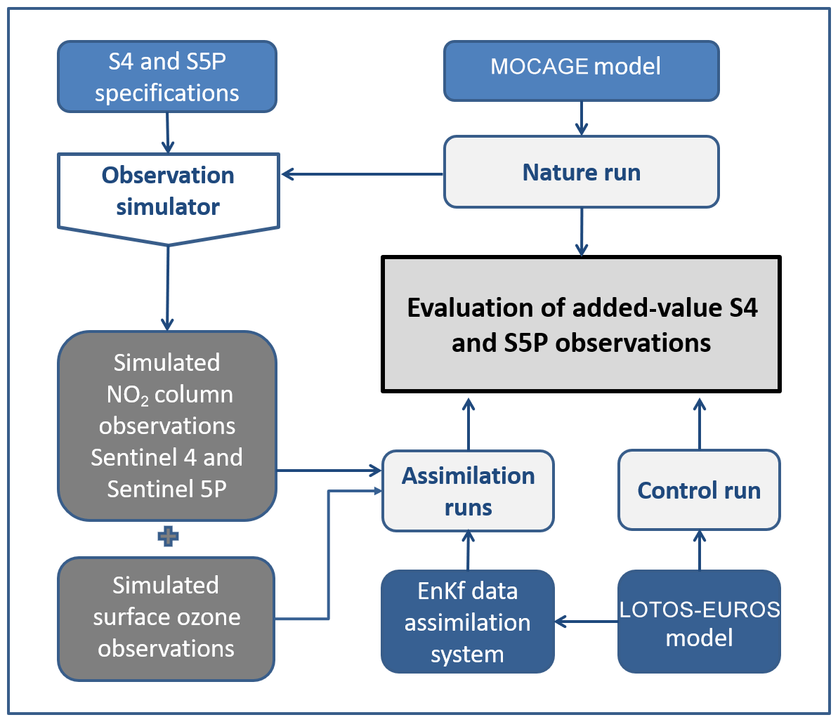
Figure 1Diagram of the Observing System Simulation Experiment components, following Timmermans et al. (2015).
We have set up the study for two 3-month study periods. The first 3-month period (June to August 2003) includes the 2003 heat wave over Europe. The stagnating weather conditions with reduced horizontal transport of the air masses and very warm temperatures lasting several days led to highly elevated levels of ozone and CO. At the same time, the chosen timeframe also covers normal conditions, allowing us to look at the full range of pollution levels occurring in a summer season in Europe. Additionally, we chose a 3-month winter period (November 2003–January 2004) to cover different seasons and chemical situations.
2.1 Nature run
The objective of the NR is to represent the true state of the atmosphere, forming the basis for the simulation of observations. The main requirements for the NR in an air quality OSSE following Timmermans et al. (2015) are that it is produced using a high-performance state-of-the-art air quality model significantly different from the model used for the assimilation runs. The NR concentrations should show spatial and temporal variations in accordance with real representative observations, cover different seasons and an extended geographical region. The resolution should be sufficient to resolve the variability at the scale of the observations of interest.
The NR in this OSSE is performed using the MOCAGE model (Peuch et al., 1999), a chemistry transport model developed at Météo-France. The model is operationally applied at Météo-France to provide the national chemical weather forecasts (Dufour et al., 2005) and is part of the regional Copernicus Atmosphere Monitoring Service (CAMS) ensemble, which provides operational air quality forecasts and analyses on a daily basis over Europe (http://macc-raq.copernicus-atmosphere.eu/, last access: 16 September 2019). In this context, the model calculations are regularly evaluated against both observations and results from the other models in the ensemble (Marécal et al., 2015).
The NR is constructed using a two-way nested configuration: a European grid (35–70∘ N, 15∘ W–35∘ E) with a 0.2∘ × 0.2∘ horizontal resolution and a smaller regional grid (41–53∘ N, 5∘ W–10∘ E), covering France and surrounding regions, with a 0.1∘ × 0.1∘ horizontal resolution. The MOCAGE model includes 47 sigma-hybrid vertical levels from the surface up to 5 hPa. The vertical resolution is 40 to 400 m in the boundary layer (seven levels) and approximately 800 m near the tropopause and in the lower stratosphere. The anthropogenic emissions are based on the TNO-MACC I inventory (Kuenen et al., 2011), complemented by EMEP 0.5∘ × 0.5∘ shipping emissions. Biogenic emissions are fixed monthly using the Simpson approach (Simpson et al., 1995). Dynamically, the model is forced every 3 h by meteorological data from the Météo-France analysis data of the ARPEGE model (Courtier et al., 1991). The gas-phase chemistry in MOCAGE uses the RACMOBUS chemical scheme, a combination of the Regional Atmospheric Chemistry Mechanism tropospheric scheme (RACM; Stockwell et al., 1997) and the REactive Processes Ruling the Ozone BUdget in the Stratosphere stratospheric scheme (REPROBUS; Lefèvre et al., 1994).
2.2 Observation simulator
We generate NO2 tropospheric column synthetic observations using model profiles extracted from the NR model datasets. The observations are generated for the TROPOMI instrument on board the S5P satellite and the S4/UVN instrument on board the MTG-S satellite. The TROPOMI instrument is a spectrometer based on its predecessors OMI and SCIAMACHY (Veefkind et al., 2012). It measures in the ultraviolet (UV)–visible (270–500 nm), near infrared (NIR, 675–775 nm) and short-wave infrared (SWIR, 2305–2385 nm) wavelength ranges to enable the retrieval of several air quality data products, including ozone, NO2, formaldehyde, SO2, methane and CO. The instrument has a wide swath of 2600 km, allowing daily global coverage and was designed for a spatial resolution of 7 by 7 km. After our study and the launch of the instrument, the spatial resolution was further improved to 7 by 3.5 km. The S4/UVN instrument (ESA, 2018a) is a spectrometer measuring in the UV (305–400 nm), visible (400–500 nm) and NIR (750–775 nm) wavelength ranges. Over Europe, it will have a spatial resolution of 8 km and an hourly temporal resolution.
The generation of the synthetic observations involves the following steps.
- i.
The generation of the MTG-S (for S4) and S5P orbits, geolocations of the individual high-resolution observations, and their corresponding geometrical properties (solar, viewing and azimuth angles). We do this for the appropriate overpass time (S5P) or observation time (S4).
- ii.
Based on the cloud distribution of the European Centre for Medium-Range Weather Forecasts (ECMWF) weather model analyses, we simulate effective cloud fractions as would be observed by the satellite.
- iii.
We generate lookup tables to compute the scene-dependent averaging kernels and observation uncertainties.
- iv.
We interpolate the NR fields in space and time to the observation footprints to derive a set of synthetic observations for the 3 summer months and the 3 winter months.
We discuss in more detail below the individual steps performed for the TROPOMI instrument on board the S5P satellite and the S4/UVN instrument on board the MTG-S satellite.
2.2.1 Orbit simulator
We simulate the geometry of the S5P and MTG-S (for S4) orbits and field of view using the System Tool Kit (STK, developed by AGI, http://www.agi.com/products/, last access: 16 September 2019). For S5p, using the orbit characteristics, the STK provides the time-dependent geolocation of the edges of the swath. Based on the location of the edges, we compute the coordinates of the individual observations assuming a spatial resolution of 7 × 7 km2 at nadir. We first compute the geometry of one S5P orbit and then apply appropriate time and longitude shifts to obtain all the orbits needed for both study periods. Subsequently, we compute the geometry for each individual observation (the solar, viewing and azimuth angles). Note that normally the size of the footprints away from nadir increases roughly by 1∘ per viewing angle. For S5P the size of the real footprints at the edges of the swath are reduced by a factor of 2 by changing the binning, leading to a more uniform footprint size across track. The footprints of the generated synthetic observations are 7 km at nadir up to ∼8.5 km at the edges. This is not fully realistic but approximates the real footprints when using the binning. For S4 the viewing angle decreases with latitude, and pixels become stretched from roughly 7 km in a north–south direction at 40∘ N up to 25 km at 70∘ N.
As a final step, we store only the part of the orbit that has an overlap with the model domain. The data are stored in formatted files that mimic the format of current NO2 column products from satellite retrievals.
2.2.2 Cloud, temperature and surface albedo information
The satellite measurements of S4 and S5P, once available, will be used to retrieve cloud properties like cloud fraction and cloud pressure, using either the O2-A band (Wang et al., 2008) or the O2-O2 absorption feature around 477 nm (Veefkind et al., 2016). However, for an OSSE those need to be estimated differently. For this purpose we take cloud information and other relevant model fields from the ECMWF weather forecast archive for the two 3-month study periods at a resolution of 0.25∘. The retrieved fields are temperature, pressure, liquid and ice water content, specific humidity, and cloud fraction. To simulate the cloud parameter observations, we convert the ECMWF cloud quantities to cloud optical properties, which determine the reflectance at the top of the atmosphere. Based on these reflectances, we simulate the effective cloud fraction and effective cloud top height similar to the procedure in the O2-O2 cloud retrieval. The distribution of effective cloud fractions obtained in this way was compared with OMI O2-O2 cloud observations for the year 2006, and a reasonable qualitative agreement of the histograms was found for summer and winter months, with somewhat fewer cloud free days and more intermediate cloud fractions in the OMI dataset, which could in part be due to the above-average number of sunny days in 2003 (Williams et al., 2013). We use the simulated effective cloud fraction and cloud pressure in the synthetic retrievals.
We convert the cloud fraction into a cloud radiance fraction (the fraction of the top-of-atmosphere radiance coming from the cloud-covered part of the scene) by computing radiances using the surface albedo map and assuming a cloud albedo of 0.8. The surface albedo is taken from the 5-year OMI Lambertian reflectivity dataset, extended from the 3-year dataset published by Kleipool et al. (2008). Figure 2 shows an example of the cloud radiance fraction simulated in this way for the 13:30 LT (local time) afternoon overpass of S5P on a day with mainly cloud-free conditions over continental Europe.
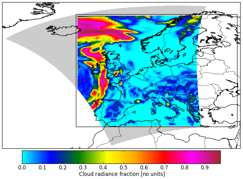
Figure 2Example of the distribution of cloud radiance fractions for the simulated S5P 12:34 UTC overpass on 1 June 2003. The rectangle represents the European modelling domain.
2.2.3 Averaging kernel lookup tables
The ideal approach for the generation of synthetic observations would involve the following steps: (1) use the NR profile and radiative transfer model to simulate radiances at the top of the atmosphere, (2) add noise to the simulated radiances based on the satellite specifications, (3) apply the retrieval approach to the simulated radiances, and (4) add extra noise related to uncertainties in retrieval parameters such as cloud fraction and surface albedo. Due to the large number of observations provided by the Sentinels, this approach is not feasible.
Following Rodgers (2000), we note that applying the forward radiative transfer model, followed by the retrieval is equivalent (after linearisation) to applying the kernel matrix A, and the synthetic observations xr can be generated with the equation , where xa is the a priori column or profile, and ϵ is the error due to the instrument and retrieval errors. As shown by Eskes and Boersma (2003), for differential optical absorption spectroscopy (DOAS) column retrievals , and the equation simplifies to . Here x is the true vertical profile of NO2 and the averaging kernel is a 1-D vector. For the DOAS column retrievals considered here, we compute the elements of the averaging kernel from the height-dependent air-mass factors (AMFs) or box AMFs (Eskes and Boersma, 2003).
Using the radiative transfer toolbox DISAMAR (Determining Instrument Specifications and Analysing Methods for Atmospheric Retrieval; de Haan, 2012), we generate lookup tables for the box AMFs for the range of geometries of the S4 and S5P. Results are stored for 21 pressure levels between 1050 and 0.1 hPa, 9 surface albedos, 10 cloud surface pressures, 10 solar zenith angles, 15 viewing zenith angles, and 3 relative azimuth angles. We use linear interpolation to find the AMF values for the satellite geometries.
2.2.4 Observation uncertainties
The Sentinel-4–5 Mission Requirements Traceability Document (ESA, 2017) specifies signal-to-noise ratios for Sentinel-4 and Sentinel-5(P). With the DISAMAR tool, we can translate these irradiance and radiance requirements to NO2 retrieval uncertainties using either DOAS or optimal estimation. We experimented with this but found that the uncertainty estimates are very sensitive to assumptions on spectral correlations in the noise. For the final set of simulations, we adopted the DOAS approach following an early version of the TROPOMI NO2 Algorithm Theoretical Baseline Document (ATBD) (van Geffen et al., 2014). We base this approach on our experience with the OMI instrument. We extrapolate the uncertainty estimate for TROPOMI from the OMI DOAS slant column retrievals and obtain an absolute estimate of 0.7×10¹⁵ molecules cm−2 for NO2 (of the order of 10 % for moderately polluted conditions) for the slant column, nearly independent of geometry or latitude. We use this estimate in the retrievals.
Other uncertainties due to retrieval input parameters, affecting the AMFs, are propagated through the DOAS equations following the approach described in Boersma et al. (2004). We assume fixed uncertainties for the cloud pressure (50 hPa), the cloud fraction (0.02) and the surface albedo (0.015). We do not explicitly model the stratospheric NO2 distribution but implicitly assume that a method will be adopted to estimate the stratospheric column, so that for the synthetic observations only the uncertainty of the stratospheric estimate needs to be accounted for. Again, based on our experience with OMI, SCIAMACHY and GOME-2 (van Geffen et al., 2014), the stratospheric vertical column uncertainty resulting from this procedure is set to 0.15×10¹⁵ molecules cm−2 or about 6 % of an average mid-latitude stratospheric column.
2.2.5 Synthetic observations
We compute the synthetic observations by applying the averaging kernels to the values from the NR linearly interpolated to the locations from the orbit simulator. We add Gaussian noise to the retrievals making use of the estimated retrieval uncertainty (Sect. 2.2.4). Figure 3 gives an example of one 13:30 LT overpass of S5P, based on the NR of 1 June 2003. Figure 3c shows the MOCAGE NR tropospheric column amount. Due to the wind from the south, there is transport of pollution from the Benelux over the North Sea. We show the uncertainty modelled in the synthetic retrieval in the Fig. 3b. We determine the detection limit noise level by combining the slant column noise with the stratospheric column uncertainty. The AMF retrieval errors related to cloud and albedo scale linearly with the retrieved column and are of the order of 25 %–50 %.
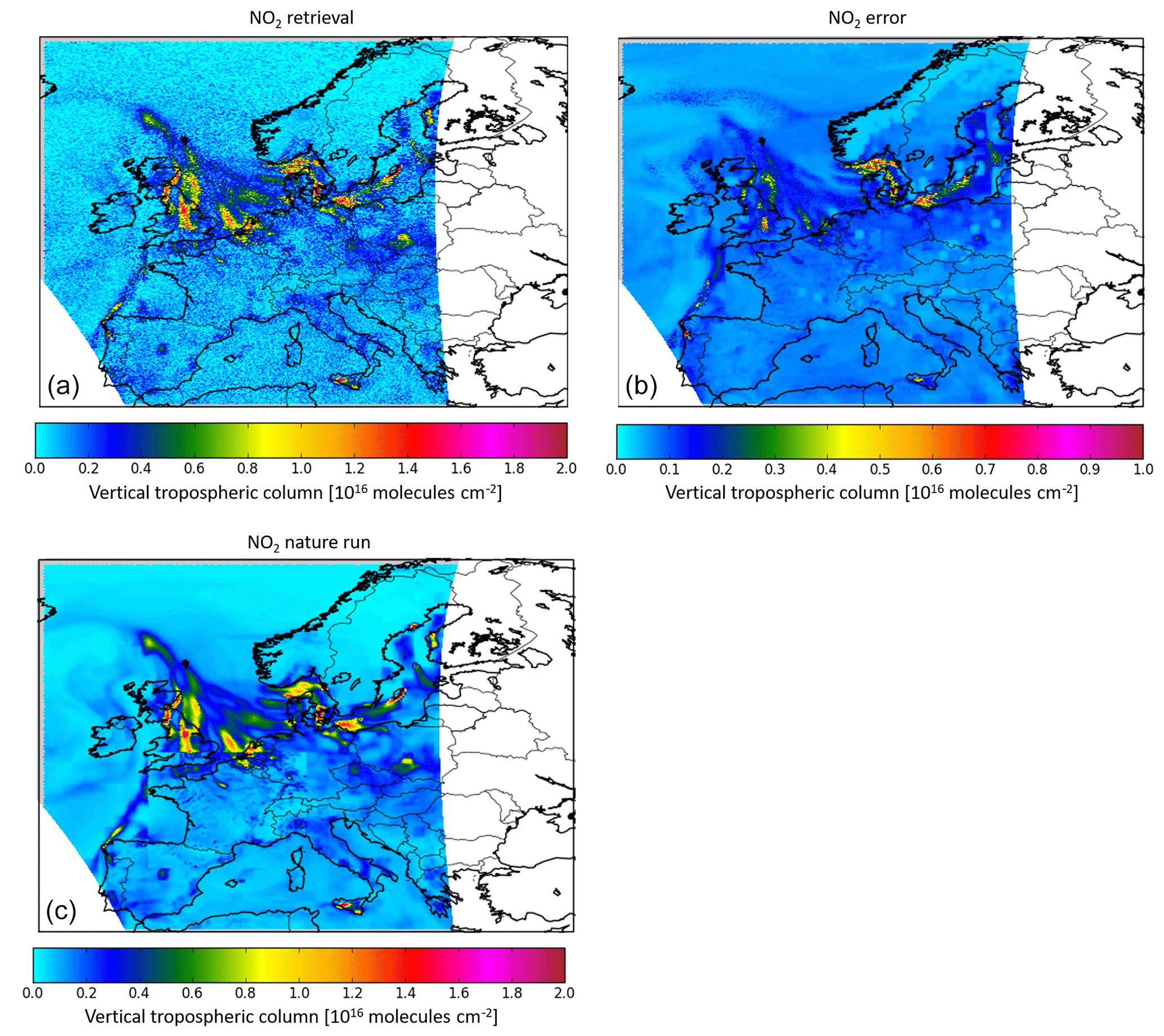
Figure 3Example of the S5P synthetic retrieval of the NO2 tropospheric column on 1 June 2003. The plots show the retrieved noisy NO2 column (a), the associated retrieval error (b) and the NR result (c).
S4 will fly on a geostationary platform; this will provide additional diurnal information about NO2. We simulate the S4 observations each hour during daytime. Figure 4 provides an example of the S4 observations as simulated, one in the early morning 04:00 UTC and one during midday at 12:00 UTC. The images demonstrate the large diurnal cycle present in the MOCAGE NR of NO2.

Figure 4Example of two S4 NO2 scenes: early morning at 04:00 UTC and midday at 12:00 UTC, on 1 June 2003. Data is plotted for solar zenith angles <85∘.
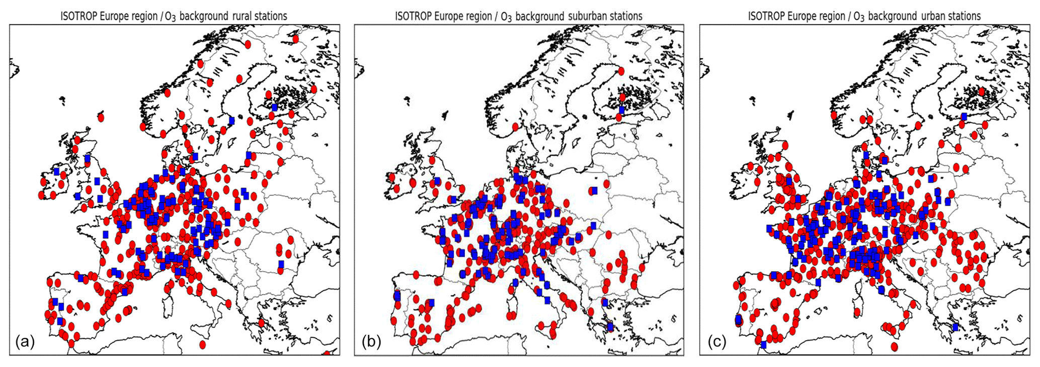
Figure 5Map of the sampling location for the ozone stations for the European region: (red circles denote assimilation stations and blue squares denote validation stations) (a) rural background stations, (b) suburban background stations and (c) urban background stations.
2.3 Synthetic ground observations
To determine the added value of the new instruments, we evaluate the benefit of the new observations on top of the benefit from observations used in the current operational system. At the time of this study, only ozone observations from monitors at the surface were used in the LOTOS-EUROS operational forecasts. Ground-based NO2 observations were not included as they measure NO2, being affected by contamination from other oxidised nitrogen species: peroxyacetyl nitrate (PAN) and nitric acid (HNO3) (Giordano et al., 2015; Steinbacher et al., 2007). Ozone assimilation influences NO2 through chemistry and through adjusted NOx emissions (see Sect. 2.5.1).
Synthetic ground-based ozone observations have been produced from the NR results to be consistent with the simulated satellite observations. We assume the network of currently existing stations for ozone is representative for the locations that will be available during the upcoming satellite missions. Therefore, the observation locations of the synthetic surface ozone observations have been drawn from the existing AirBase network (version 6, Simoens, 2012). We only use stations classified as “background”, since these are representative for concentrations at the resolution of the models used in this study. Additionally, we omit stations above 700 m above sea level, considering the focus of the project on boundary layer concentrations and the difficulties models have reproducing conditions in mountainous areas. Figure 5 shows the location of the selected stations. During data assimilation experiments, it is common practice to leave a number of observations out of the assimilation procedure and use these for validation. The split of observations used and presented in Fig. 5 is taken from the MACC II project (Marécal et al., 2015). We use only the locations of stations labelled as assimilation stations. We sample the ground-based synthetic observations from the lowest-level NR output by performing a bilinear horizontal interpolation to the selected station locations.
One of the most important quantities in an assimilation system is the representation of the variance of the departures, which quantifies differences between an observation and its forecast by the model. These differences arise due to a combination of instrumental errors, the grid cell formulation used in a model, deficiencies in the simulated processes and other errors. Proper quantification of the representation error, related to the mismatch of the point measurement and the model grid and effective resolution of the model, is a major task in an assimilation exercise. Generally, we base its estimate on comparison of the observations and model simulations. The only exception is determination of the measurement error, which is solely dependent on the instruments. However, in air quality databases like AirBase, it is not common practice to provide characteristics of instrumental errors (while retrieval uncertainties are provided for individual observations in the case of satellite measurements). Therefore, the error of ground-based observations should be set or parameterised explicitly (e.g. Thunis et al., 2013)
To ensure realistic synthetic surface ozone observations, we mask the synthetic ground-based observations if the corresponding real observations in AirBase are missing too. Secondly, we add a random number to each synthetic value to represent the instrumental error. We base the distribution of this random number on statistics obtained from the AirBase observations available for the same period. More specifically, we determine the temporal auto-covariance in a time series of ozone observations. The difference gap from variance (lag zero) to the first covariance (lag one) is then a measure of the random hour-to-hour variation. This variation therefore represents both instrumental errors as well as variations on timescales of less than an hour.
2.4 Control run
The CR in the OSSE is performed using the LOTOS-EUROS model, a chemistry transport model developed by TNO (Manders-Groot et al., 2016; Manders et al., 2017). The model provides the national Dutch operational chemical weather forecasts (https://www.lml.rivm.nl/verwachting/animatie.html, last access: 16 September 2019) and is part of the regional CAMS ensemble, which provides operational air quality forecasts and analysis on a daily basis over Europe (http://macc-raq.copernicus-atmosphere.eu, last access: 16 September 2019). In this context, the model calculations are regularly evaluated against both observations and results from the other models in the ensemble (Marécal et al., 2015). The objective of the model is to describe air pollution in the lowermost atmosphere; to achieve this, the standard version has four vertical layers following a dynamical mixing layer approach. The first layer is a fixed layer of 25 m thickness; the second layer follows the mixing layer height. We evenly distribute the remaining two reservoir layers between the mixing layer height and 3.5 km. The implicit assumption of the LOTOS-EUROS model is the presence of a well-mixed boundary layer, i.e. constant concentrations between the surface layer and the mixing layer height.
The CR is constructed using a nested configuration: a European grid (Europe: 35–70∘ N, 15∘ W–35∘ E) with a 0.125∘ × 0.25∘ resolution in the longitudinal–latitudinal direction and a smaller regional grid (zoom: 41–53∘ N, 5∘ W–10∘ E) with a 0.0625∘ × 0.125∘ resolution in the longitudinal–latitudinal direction. The lateral and top boundary conditions for the European grid are taken from a global reanalysis by the TM5 model (Huijnen et al., 2010; Williams et al., 2017). The same TM5 model runs are also used for the extension of the LOTOS-EUROS runs from its top at 3.5 km to the tropopause.
We base the anthropogenic emissions on the TNO-MACC II inventory (Kuenen et al., 2014). Note this is a different inventory version than used in the NR, supporting the requirement of significant differences between the models for the NR and the CR and AR. Biogenic emissions are calculated online as described in Schaap et al. (2009). Fire emissions are taken from the MACC-II GFAS v1.0 product (Kaiser et al., 2012). These emissions vary from day to day and are provided on a 0.5∘ resolution grid. Dynamically, we force the model by meteorological data from ECMWF. We choose a different meteorological forcing from the one used in the NR to meet the requirements on the differences between the NR and the CR and AR. The gas-phase chemistry in the LOTOS-EUROS model is based on a modified version of the CBM-IV mechanism. We refer to Manders-Groot et al. (2016) and Manders et al. (2017) for more details on the emission speciation and corresponding lumping to the chemical mechanism species.
2.5 Assimilation runs
To evaluate the benefit of the S4 (GEO) and S5P (LEO) NO2 observations for air quality analyses, we assimilate the synthetic observations into the LOTOS-EUROS model. We use different configurations to evaluate the individual and combined benefits of the GEO and LEO satellite instruments. We evaluate the benefit of the new observations against a reference situation where we assimilate only ground-based ozone observations.
2.5.1 Data assimilation system – ensemble Kalman filter
The LOTOS-EUROS set-up features an active data assimilation system based on the ensemble Kalman filter (EnKf) technique (Evensen, 2003). A Kalman filter computes probability density functions (pdf's) of the true state, given (1) a transition model to propagate the state in time with associated uncertainties and (2) observations with associated representation error. Starting from the initial pdf, the filter first performs a forecast step propagating the pdf in time until the first moment that observations become available. Then, during the analysis step, we replace the forecast pdf with an analysed version that takes into account the new information available. The Kalman filter is an example of sequential assimilation, since forecast and analysis steps follow each other sequentially in time and use only information from the past. To be able to apply this technique to a large-scale air quality model, the pdf is described by an ensemble of model states in a so-called EnKF (Evensen, 2003). The spread between the ensemble members should describe the uncertainty in the state quantities as the mean and covariance of the state is computed from the ensemble statistics. The number of required ensemble members depends on the complexity of the pdf, commonly determined by the non-linearity of the transition model and the complexity of the associated model uncertainty. In practice, an ensemble with 10–100 members is acceptable to keep computations feasible. The data assimilation system in LOTOS-EUROS has been successfully applied for assimilation of O3, NO2, SO2, and aerosol observations from either ground-based or satellite instruments (Barbu et al., 2009; Curier et al., 2012; Eskes et al., 2014; Fu et al., 2017; Schaap et al., 2017; Segers et al., 2010; Timmermans et al., 2009).
2.5.2 Assimilation parameter settings
The ensemble specification has a number of settings that need to be set prior to the assimilation experiments. These include the selection of uncertain model parameters (e.g. emissions), the amplitude of the assumed uncertainties and their temporal correlation. Additionally, the assimilation system requires a number of other parameters to be set that influence the results: ensemble size, localisation length scale for different types of observations and representation error covariance. The latter quantifies the differences caused by the different resolutions of the model and the observations.
In this study, we use the selection of model parameters as used in the operational national and European CAMS forecasts, which are the emissions of the ozone precursors (NOx and non-methane volatile organic carbons, NMVOCs), deposition velocity of ozone and the boundary conditions for ozone, all with an assumed uncertainty of 50 % and assumed temporal error correlation of 1 d.
The localisation length scale for the ground-based ozone observations is set to 50 km following Curier et al. (2012). The length scale for assimilation of the synthetic NO2 observations has been set to 0 km.
We base the representation error covariance for the satellite observations on observation minus simulation statistics and spatial correlations present in the observations. We obtain the representation error for the surface ozone observations by analysing the impact of spatial averaging. This depends on the spatial variance in the ozone fields, i.e. higher at coastlines and in mountain areas where we find the highest ozone gradients.
An important parameter in the filter is the ensemble size. In general, the ensemble size should be large enough to represent the covariance structure imposed by model uncertainties and the model physics. In this application, the covariance structure is rather simple, since we describe all uncertainty by the local sources, and observations are available regularly over the domain. With the chosen configuration, we show that an ensemble size of 12 members is sufficient to obtain stable results.
2.5.3 Observation data handling
Within the data assimilation system, the synthetic observations are ingested using their estimated uncertainties. The available averaging kernels from the synthetic observations are applied to the model profiles from the surface to the tropopause to make them comparable to the column observations from satellites.
In case the assimilation system is unable to represent an observation correctly, the assimilation may lead to instability of the system. Such an instability can occur if the model lacks certain physical parameterisations or if the model is unable to represent a measurement resulting in a mismatch of the model and measurement spatial or temporal resolution. To avoid this, we apply a screening procedure to reject those measurements that cannot be represented correctly by the assimilation system. The screening procedure is taken from Järvinen and Undén (1997). If the square of the difference between observation and filter mean is more than a factor of 3 larger than the expected variance of this difference, we reject the observation.
In addition, we filter out all synthetic observations with cloud radiance fraction higher than 50 % (to exclude cloudy pixels) and those with surface albedo higher than 0.3 (the high reflectance complicates the NO2 retrieval and for OMI data users are advised to discard scenes with surface albedo values >0.3; Boersma et al., 2011). All observations within the model grid cells are averaged before assimilation using weights according to overlap between pixel footprint and grid cell.
2.5.4 AR configurations
Table 1 provides an overview of the different configurations of the assimilation runs. The runs with assimilation of synthetic surface ozone observations only serve as reference runs to represent current operational system capabilities. The runs with assimilation of GEO, LEO, or GEO and LEO observations combined serve to evaluate the added value of the new satellite instruments under study. We perform these runs for a European, zoom and fire domain, as presented in Fig. 6. The fire domain covers part of the Iberian Peninsula and is only included in a run for a short episode (first 2 weeks of August 2003) with large fires in Portugal.
Table 1Overview of assimilation run configurations. RR: reference run; OR: assimilation run; F: fire domain; Z: zoom domain; E: European domain; GN: GEO satellite; LN: LEO satellite; LGN: LEO and GEO satellite.


Figure 6Illustration of different domains used for the assimilation runs. European domain (red rectangle), zoom domain (blue rectangle) and fire domain (purple rectangle).
2.6 Evaluation method
The goal of this study is the quantitative assessment of the added value of the S5P and S4 NO2 observations on surface air quality analyses. We performed statistical analysis of the assimilation runs in comparison to the NR to achieve this goal. During the statistical analysis, we use the following diagnostics:
-
mean bias:
-
root-mean-square error:
-
temporal correlation:
-
normalised mean bias:
-
mean absolute error:
-
normalised mean absolute error:
Here X is the array of modelled values from CR, RR, or AR; NR is the array of values from the nature run; and N is the number of values over which we calculate the mean. The value of N varies between the different plots.
3.1 Evaluation of nature run and control run
In the design of an OSSE, it is important to demonstrate that the NR exhibits the same statistical behaviour as the real atmosphere for aspects relevant to the observing system under study. To evaluate this, we compare the ozone and NO2 concentrations from the NR to observations from the AirBase network. We consider the sites falling into the first five classes, as defined in the objective classification method suggested by Joly and Peuch (2012), as we understand them to be representative for the resolution of the NR model. These first five classes mostly encompass sites classified as rural and urban background in the AirBase database but, especially for ozone, a small fraction of the urban traffic stations have also been assigned to one of the five lowest classes and are therefore considered representative for larger areas. Figure 7 shows that, for ozone, the NR exhibits similar day-to-day and diurnal variability as the observations. On most days, the model underestimates the afternoon ozone peak, although on some days, the peak is overestimated. For NO2, an underestimation of observed levels is obvious. This could, among other reasons, be due to an underestimation of the emissions prescribed to the model and/or an overestimation of the vertical mixing. Additionally, the NO2 observations likely overestimate ambient NO2 concentrations due to contamination from other oxidised nitrogen species such as PAN and HNO3 (Giordano et al., 2015; Steinbacher et al., 2007). Despite the bias, the temporal behaviour of the modelled NO2 concentrations from the NR seems to resemble the temporal behaviour of the observations with the lowest values during daytime when dilution is strongest and chemical lifetime of NO2 is shortest and higher values during the night (see Fig. 8). Furthermore, day-to-day variations are reproduced, e.g. the maxima being higher in the second week of July than in the first week.
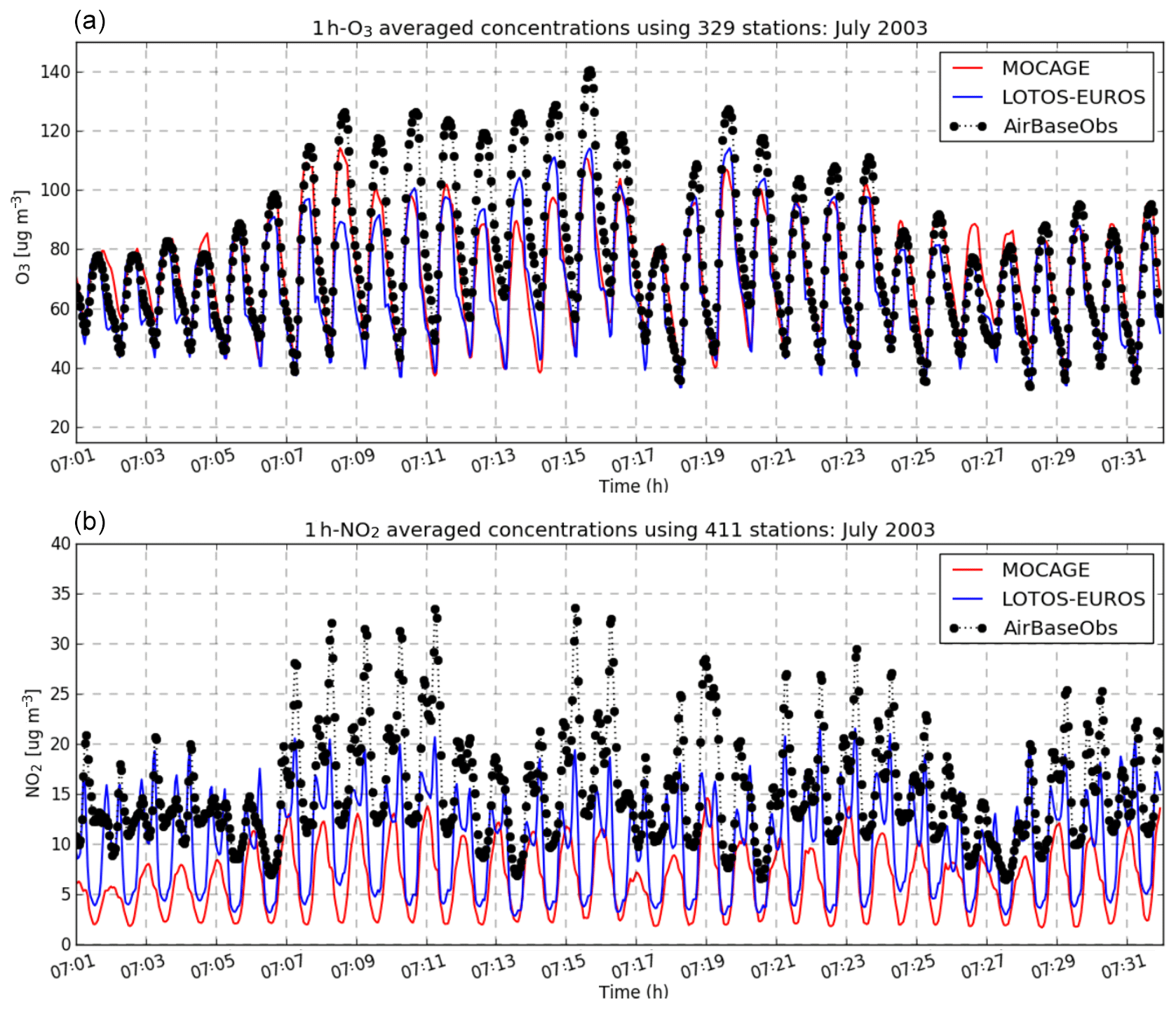
Figure 7Time series of ozone (a) and NO2 (b) concentration from NR (red, MOCAGE), CR (blue, LOTOS-EUROS) and AirBase background observations (black dots) for the period of July 2003.
Figure 8 shows the diurnal cycle from CR, NR and observations averaged over all selected locations for August 2003. For ozone, all three datasets show similar diurnal variation with the lowest values in the early morning and an afternoon peak. The models do show an underestimation of the observed ozone values. This bias is regionally dependent (not shown), with larger negative values for southern Germany and central France, small biases over the Netherlands, and even positive biases in the MOCAGE model over some periods in northern Germany. For NO2, the NR from the MOCAGE model is missing the early morning peak due to the morning rush hour when the boundary layer is still shallow and photolysis is still limited. However, considering the daytime hours where satellite observations will be available, the temporal behaviour is comparable, decreasing towards early afternoon and increasing towards the evening.

Figure 8Diurnal cycle for ozone (a) and NO2 (b) concentrations from NR (blue, MOCAGE), CR (red, LOTOS-EUROS) and AirBase background observations (black dots) for the period of August 2003. The vertical bars represent the standard deviation over the dataset (different days and stations).
Regarding the spatial variability, the NR shows strong gradients around large source areas, i.e. cities (e.g. Paris), ports, shipping lanes and highly populated areas with a lot of traffic and industry (e.g. the Benelux and the Ruhr area) (see Fig. 3c and Fig. 9). This spatial variance is representative of observations from both ground-based observations and satellite observations. We would like to note that the resolution of the NR and synthetic satellite observations (7 by 7 km) is not representative for locations with large sources and high spatial variability at scales <7 km, therefore not all ground-based observed variations can be represented.
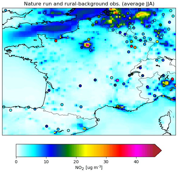
Figure 9Average NO2 concentrations over zoom domain for NR (background) for summer study period. Coloured dots indicate averaged real observation values.
From the comparisons with real observations, we conclude that the NR is representative of the variability of actual observations over Europe, albeit with a negative bias for both surface O3 and NO2. For the robustness of the OSSE such a negative bias is acceptable as long as the absolute differences between the CR and NR are comparable in size to absolute differences between state-of-the-art models and real observations. This requirement for sufficient differences between the NR and the CR is an important constraint to avoid the identical twin problem (Arnold and Dey, 1986). Ideally, the differences between NR and CR should show similar features as the differences between the CR and real observations. In Figs. 7 and 8 the O3 and NO2 concentrations from the CR (without any assimilation) are plotted in comparison to the NR concentrations and the real AIRBASE observations, respectively. During daytime the differences between the CR and NR are within the same range of values as the differences between CR and the real observations. In the middle of the day, around the overpass time of the S5 mission, the differences between the CR and the NR are somewhat smaller than between the CR and the real observations, especially for NO2.
For NO2 we assimilate satellite columns, therefore the requirement for avoiding the identical twin problem should also be checked for the column values. The bias in the summer study period NO2 columns between CR and synthetic NO2 columns varies between and 10×1015 molecules cm−2 (see Fig. 10a, c). The largest biases are seen over the main source areas and most regions exhibit a bias of around 2×10¹⁵ molecules cm−2. Average bias in daytime is between 1 and 2×10¹⁵ molecules cm−2 for both summer and winter study periods (not shown). For the summer study period and zoom domain, the average root-mean-square error (RMSE) is around 6×10¹⁵ molecules cm−2 (see Fig. 12a, black line), for the entire European domain it is somewhat lower and for the winter study period it is slightly higher (not shown). These values are comparable to values found in Curier et al. (2014), where LOTOS-EUROS model results have been compared to OMI tropospheric NO2 columns over a 6-year period from 2005 to 2010. In that study, the average biases for different domains and periods is 1–2×10¹⁵ molecules cm−2. The RMSE distribution over Europe averaged over the entire 6-year period varies between 0 to 10×1015 molecules cm−2, similar to our CR differences with the synthetic observations. The bias between CR and synthetic NO2 columns is also comparable to biases of 0.3 to 2×10¹⁵ molecules cm−2 found between the regional CAMS model ensemble and Multi-Axis Differential Optical Absorption Spectroscopy (MAX-DOAS) surface observations of NO2 columns (Blechschmidt et al., 2017).

Figure 10Summer period (JJA 2003) average NO2 column bias at 14:00 UTC, with synthetic observations for the control run without assimilation (a, c) and with assimilation (b, d) of ground-based O3 + S4 NO2 (b) and ground-based O3 + S5P NO2 (d).
Based on above analyses on the realism of the NR and on the differences between CR and NR, we conclude that the main requirements to ensure a robust and realistic OSSE are fulfilled.
3.2 Evaluation of OSSE results
3.2.1 NO2 columns
Figure 10 shows the bias around time of overpass of S5P (over central Europe at 14:00 UTC) between modelled NO2 columns and the synthetic NO2 observations from the CR without any assimilation and the ARs with assimilation of either S4 or S5P data averaged over the summer period June–July–August (JJA) in 2003. The CR overestimates the NO2 columns, especially over the Benelux, the Ruhr area in Germany and the south-eastern part of the UK. These regions are characterised by high NO2 concentrations due to high density of sources such as traffic, shipping and industry. A strong decrease in the bias is visible after assimilation of the synthetic Sentinel data in combination with ground-based ozone observations. On average, the impact of the S4 and S5P observations in combination with the ground-based observations is very similar at the overpass time. Note that in the eastern part of the domain, the bias is not zero for the S5P case, but observations do not cover this region around 14:00 UTC. Figure 11 shows that the temporal correlation improves by the assimilation of the Sentinel observations. Over large parts of the domain and especially the areas with high NO2 concentrations, the temporal correlation increases significantly. Considering the overpass time, the temporal correlation in this case is a measure of the representation of the day-to-day variability. This result shows that the system is working as expected and the data assimilation pulls the modelled values towards the observations.
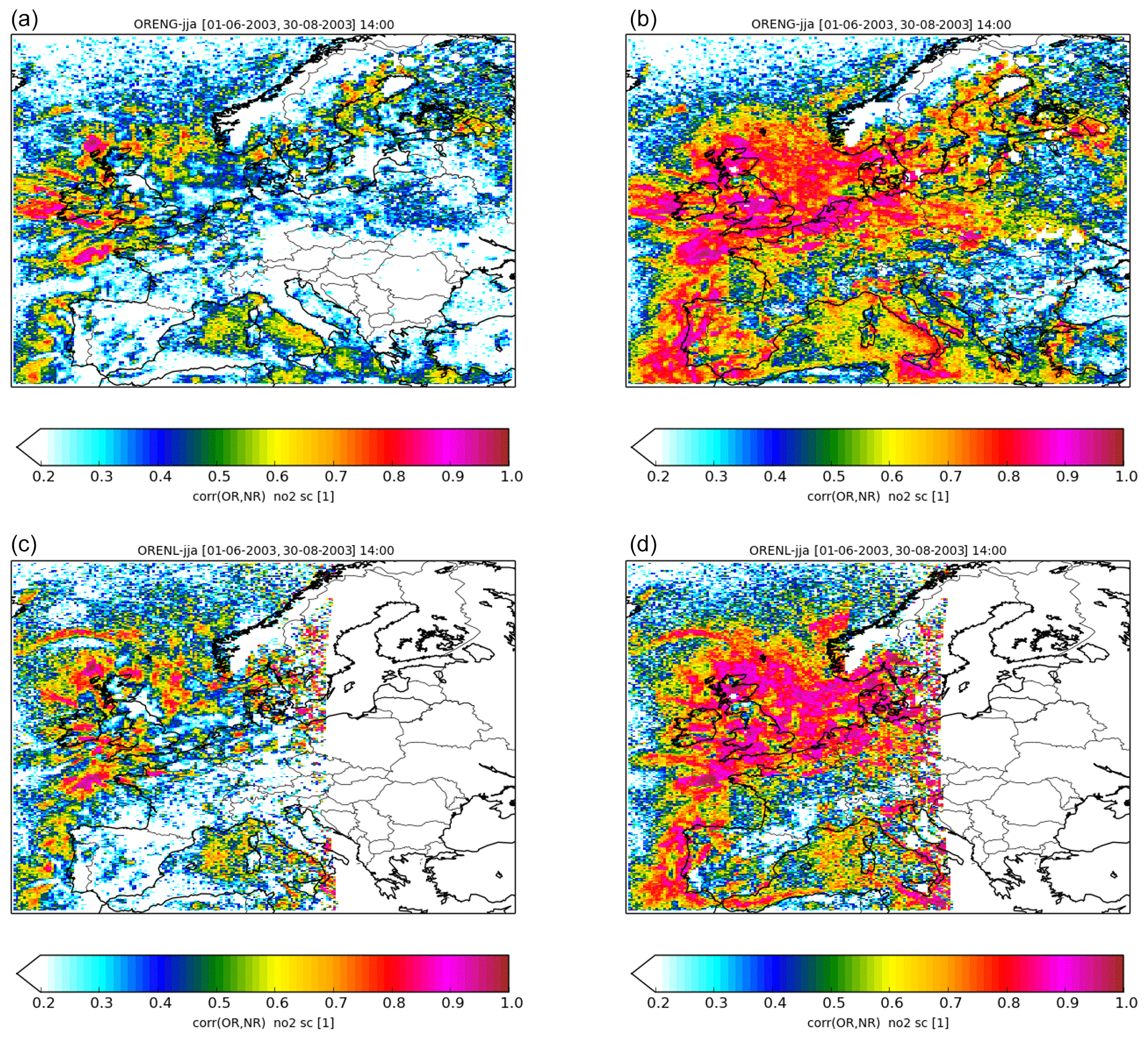
Figure 11Summer period (JJA 2003) temporal correlation of modelled NO2 columns at 14:00 UTC with synthetic observations for the control run without assimilation (a, c) and with assimilation (b, d) of ground-based O3 + S4 NO2 (b) and ground-based O3 + S5P NO2 (d).
For the winter period, the conclusion is the same as for the summer period: bias and RMSE decrease while the temporal correlation increases (not shown).
To evaluate the added value on top of the ground-based observations, we compare the results with the reference run (RR), where we assimilate only ground-based observations. Figure 12a and b shows the statistical evaluation for the high-resolution zoom domain as function of the time of the day, for the modelled NO2 column. We see that for the modelled NO2 columns, the assimilation of ground-based ozone observations in the RR during the summer study period leads, on average, to a negative impact on RMSE (an increase) during the night and on correlations throughout the entire day. Further investigation demonstrates that the assimilation of the ozone observations improves the surface ozone concentrations. The reason for this negative impact on NO2 column may lie in the fact that the errors in modelled surface ozone concentrations and in modelled NO2 columns are not dominated by the same error source. Another reason could be that the assimilation system is not adapting the dominant parameter responsible for both the ozone and NO2 column errors. Remember there are four uncertain model parameters in the set-up used in this study that can be adapted through the assimilation. Assimilation of observations should, therefore, always be evaluated with care and one should analyse individual impacts of observation sets or impacts on different components.
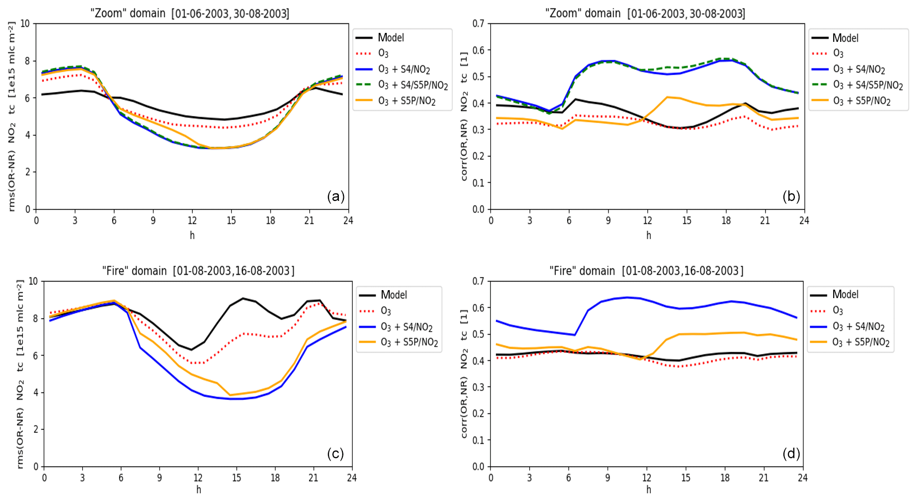
Figure 12RMSE (a, c) and correlation (b, d) with NR tropospheric NO2 column for the summer period and zoom domain (a, b) and the fire episode (1–16 August 2013) and domain (c, d). Prior to (black line) and after assimilation of observations (coloured lines – ground-based O3 only: dotted red; ground-based O3 + S4 NO2: blue; ground-based O3 + S5P NO2: yellow; and ground-based O3 + S4 and S5P NO2: dashed green).
The additional assimilation of satellite NO2 column observations improves the RMSE and correlations in NO2 columns in comparison to the RR. This impact is clearer in the results focusing on the fire episode over the Iberian Peninsula (Fig. 12c and d). The impact of the GEO S4 observations is visible throughout the entire day, while the impact of the LEO observations at the overpass time is smaller than the impact of the S4, which continuously feeds the model and lasts for several hours. The combined assimilation of S4 and S5P observations for the zoom domain only, minimally increases the correlation around the overpass time of S5P in comparison to the assimilation of S4 data only and does not show a benefit on the RMSE.
3.2.2 NO2 surface concentrations
While the results above demonstrate that the system is working as expected and is able to decrease the difference between the model and synthetic NO2 observations, the goal of our study is to investigate the added value of the Sentinel observations for air quality analyses at the surface where the impact of air pollution is the most significant for human health and the ecosystem.
Figure 13 illustrates the impact of the assimilation on modelled surface NO2 concentrations. Here we also see a positive impact of assimilating S4 and/or S5P observations. The RMSE decreases by about 30 % during daytime hours (or from the overpass time onwards for S5P), and the correlation increases by about the same amount. On average, the impact here is slightly smaller than on the modelled NO2 column. Whereas concentrations of NO2 show very distinct high-resolution features in a small surface layer, mixing towards larger upper layers leads to less pronounced features in the column values. The observed NO2 columns, therefore, do not contain the level of detail that the surface NO2 does. The comparison with modelled NO2 columns is more direct, covers the same altitude region and therefore, as expected, shows a larger impact than the comparison with surface NO2. As the Sentinel tropospheric NO2 columns do not contain any information about the vertical distribution within the troposphere, the assimilation of NO2 columns may in some cases also lead to a deterioration of modelled surface concentrations when the vertical NO2 profiles in the model are incorrect.
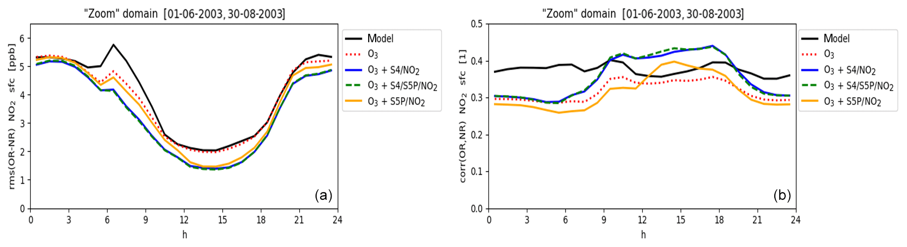
Figure 13RMSE (a) and correlation (b) with NR surface NO2 concentrations for the summer period and zoom domain. Prior to (black line) and after assimilation of observations (coloured lines – ground-based O3 only: dotted red; ground-based O3 + S4 NO2: blue; ground-based O3 + S5P NO2: yellow; and ground-based O3 + S4 and S5P NO2: dashed green).
Figure 14 shows the positive impact on modelled surface NO2 concentrations in a geographical form. This figure shows the bias of the different runs, averaged over the summer period at 10:00 UTC (shortly after the morning rush hour), for a region centred over France where traffic highways are highly pronounced. The CR overestimates the surface NO2 concentrations over traffic highways and large urban areas (e.g. Paris and London). While the ground-based ozone observations in the RR are able to decrease this positive bias, (averaged over the zoom domain from 0.8 to 0.4 ppb), the S4 observations (available throughout the day) are able to decrease this bias further over the traffic highways (average bias over zoom domain is eliminated). Furthermore, over the shipping lane through the English Channel, between the UK and France, the bias significantly decreases from values around 5 to nearly 0 ppb. The S5P, with its afternoon overpass time, has an expected negligible impact at 10:00 UTC. As could be seen in Fig. 13, at 14:00 UTC the impact of the S5P for surface NO2 concentrations is similar to the impact of S4.
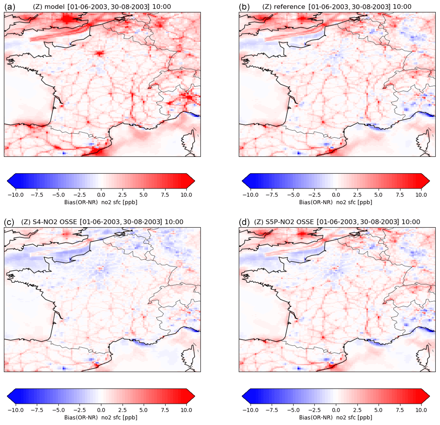
Figure 14Zoom domain: summer, 10:00 UTC average. Bias with NR surface NO2 before assimilation (a) and after assimilation of ground-based O3 (b), ground-based O3 + S4 NO2 (c) or ground-based O3 + S5P NO2.
For the winter period, the impact of the assimilation of Sentinel data on surface NO2 concentrations shows a mixed picture, which hints to the importance of the model profile shape for improvements at the surface when assimilating column observations. A mismatch between the bias in column NO2 and surface NO2 can lead to a negative impact of the satellite observations. Figure 15 shows the bias compared to the NR surface NO2 concentrations for the CR without any assimilation and the AR including the assimilation of surface ozone observations and S4 synthetic observations. The CR shows an overestimation of the NR concentrations over central Europe, large cities in southern Europe and the shipping lanes in the Mediterranean. Differently, the CR shows an underestimation of surface NO2 concentrations over the north-eastern part of the domain. The assimilation of the synthetic observations clearly decreases the modelled concentrations over the central European area and leads to a reduced bias over, for example, Germany. Over some of the eastern European countries, the concentrations increase and the negative bias decreases, for example in Romania, Ukraine and Belarus. However, these positive impacts are not present over the entire domain. Over some areas, the positive bias increases (e.g. over Austria, Slovenia and Northern Italy) or changes to a negative bias (e.g. over Barcelona, Belgium and the Netherlands). We have found that, in many of these situations, the bias in surface NO2 concentration does not match the bias in tropospheric NO2 column. For example, in the area covering Austria and Slovenia, the CR underestimates the NO2 column from the NR. Assimilation of synthetic S4 observations derived from the NR then increases the NO2 values and can only do so by increasing the sources at the surface. Even if we would only be able to increase the concentrations at higher altitudes, the satellite measurements do not provide information about the vertical profile or at which altitude the model is biased. The increased emissions at the surface then lead to even higher concentrations and an increased positive bias in this specific situation. These results demonstrate the importance of a correct representation of the vertical distribution in the model and of an evaluation of model profiles with independent profile information, for example from MAX-DOAS or aircraft measurements. In our experiment, the vertical distribution of the NR and CR in some cases differs in this way, leading to occasional negative impacts from the assimilation of the synthetic observations.
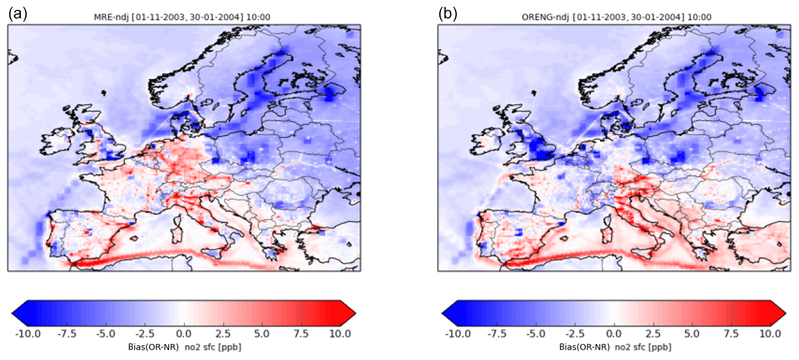
Figure 15Winter period average surface NO2 bias at 10:00 UTC with respect to the NR (in ppb) for the CR without assimilation (a) and with assimilation of ground-based O3 + S4 NO2 (b).
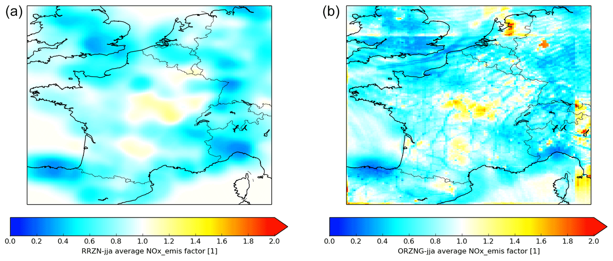
Figure 16Average NOx emission increment for the run with assimilation of ground-based ozone observations only (RR) (a) and the S4 assimilation run (b) for the summer study period over the zoom domain.
3.2.3 Emissions
We perform the OSSE in this study with an ensemble Kalman filter approach, which optimises the NO2 concentrations by specification of uncertainties in model parameters, as described in Sect. 2.5.2. The parameter that most directly influences the NO2 concentrations is NOx emissions; other parameters such as NMVOC emissions and ozone deposition velocities are more related to ozone. As an example of the change in model parameters, Fig. 16 shows average NOx emission adjustments for the summer period for the RR and AR with S4 data. The distribution of emission adjustments is quite similar between both runs, which gives confidence to the choice of uncertain parameters. The assimilation of high-resolution S4 NO2 observations has a relatively large additional impact over some areas of the domain. For example, the NOx emissions over the centre of the Netherlands increase, while the NOx emissions over the shipping route in the English Channel decrease. Due to the high resolution of the S4 data and the smaller length scale set in the assimilation, the S4 observations bring more detailed emission updates than ground-based ozone observations only. Note that this assimilation set-up, with uncertainties in the emissions, is less flexible at remote locations with small emission fluxes.
In comparison to preceding instruments (e.g. OMI), the NO2 observations from S4 and S5P bring considerable advances. These include (1) much improved resolution, from about 20 to 7 km or even higher, (2) hourly observations in the case of S4, providing full daytime sampling, and (3) foreseen improvement in the instrument (for TROPOMI an improvement of the slant column uncertainty of 30 %–40 % compared to OMI has been reported (van Geffen et al., 2018)) and improvements due to advances in the characterisation of aspects like clouds, albedo, and aerosol effects.
In this study, we perform an OSSE experiment to illustrate the added value of these new (S5P) and future (S4) observations for NO2 analyses over Europe. The OSSE experiment has been carefully designed, with separate models for the NR and AR and with conservative estimates of the total observation uncertainties. The results show that both S4 and S5P tropospheric NO2 columns have a clear positive impact on modelled NO2 values. Assimilation of these observations on top of ground-based ozone observations decreases biases and the RMSE and improves the temporal variability of modelled NO2 distributions. S4 will bring a major step forward with its hourly temporal resolution. Owing to the assimilation of synthetic S4 observations, we are able to reconstruct many of the NR features, and the benefit is present throughout the entire day due to the availability of observations at an hourly resolution. For S5P, we observe a good impact up to 3–6 h after the overpass time. Based on our results, a similar impact is expected for S5, which will have similar technical specifications but an earlier overpass time in the morning. Simultaneous availability of S5 and S5P observations in the future is expected to provide benefits throughout the entire day due to the different overpass times and benefits lasting several hours.
The added value of the satellite observations is visible in both modelled columns as well as in the surface concentrations of NO2. During the summer period over the zoom domain (Iberian Peninsula), the RMSE in surface NO2 decreases by about 30 % during daytime, while the temporal correlation increases by the same amount. The impact of both instruments on NO2 columns is even larger. In the winter period, the additional assimilation of the satellite NO2 observations counteracts the positive impact of surface ozone observations in some regions. This results from opposing effects from the bias in satellite NO2 columns and the bias in surface NO2 concentrations, due to different vertical NO2 profiles in the MOCAGE NR and LOTOS-EUROS. It is thus crucial to analyse the model performance for simulating NO2 profiles. Accurate vertical distributions in the model are a prerequisite for consistent positive results of the column data assimilation at the surface, provided there is no additional information about the vertical profile from the satellite observations.
This study focuses on NO2 analyses, which are one of the main air quality applications that make use of satellite tropospheric NO2 columns. Another common application that combines information from models with satellite observations is the derivation of emissions. The active data assimilation system based on the ensemble Kalman filter approach that is applied in this study is especially suitable when looking at applications such as emission inversions and air quality forecasts, as it updates not only the state of the atmosphere (e.g. NO2 concentrations) but also the driving input parameters (in this study the NOx and NMVOC emissions). A more detailed analysis of the impact of the Sentinel observations on the emissions would be worthwhile to assess the added value of the new NO2 column observations from S4, S5 and S5P for emission inversion applications.
In October 2017, after completion of our study, S5P has been launched and actual tropospheric NO2 columns have become available. These actual results have proven that our retrieval error estimates, as detailed in Sect. 2.2.4, are conservative due to improvements in the retrievals (van Geffen et al., 2018). For NO2, we find slant column errors for S5P to be of the order of 0.5–0.6×10¹⁵ molecules cm−2, compared to the 0.7×10¹⁵ molecules cm−2 used in this study. We assume the AMF errors, which dominate the total uncertainty for NO2 and are computed from the cloud and surface albedo uncertainties, are comparable to what we use in this study. This means that the weight given to the observations in the data assimilation will be larger with the real observations than with our synthetic observations. The calculated S5P impact on modelled analyses is therefore expected to be on the conservative side. With the arrival of the actual S5P observations we plan to compare results from assimilation of TROPOMI (S5P) NO2 columns with the results in this study. This comparison will allow evaluation of the realism of the OSSE and will provide valuable support for any future OSSE studies.
This work was part of a study funded by ESA called “Impact of Spaceborne Observations on Tropospheric Composition Analysis and Forecast” (ISOTROP), to study the impact of S4, S5 and S5P observations of ozone, CO, NO2 and HCHO on air quality analyses. The impact of assimilation of CO from these instruments is presented in Abida et al. (2017). A paper on the impact of assimilation of tropospheric ozone from the instruments is under review (Quesada-Ruiz et al., 2019).
The LOTOS-EUROS chemistry transport model is available in an open-source version for public use via https://lotos-euros.tno.nl/ (last access: 16 September 2019). The LOTOS-EUROS data assimilation code used in this study is property of TNO and not allowed to be shared publicly. The MOCAGE model is property of Météo-France and not allowed to be shared publicly.
The volume of the model and synthetic observation datasets discussed in this paper is large, but for scientific purposes subsets can be made available upon request.
RT prepared the manuscript with contributions from all authors. RT, MS, LC, HE, WL and JLA designed the experiment and provided scientific guidance during the project. AS and LC developed the LOTOS-EUROS code and performed the OSSE assimilation runs. RA, JLA, LEA, SQ and PR developed the MOCAGE model code, performed the MOCAGE nature run and produced the synthetic ground-based ozone observations. JdH, PV, HE, JK and AON produced and provided the synthetic NO2 observations. RT, MS, AS and HE performed the analyses of the model assimilation runs.
The authors declare that they have no conflict of interest.
We would especially like to thank William Lahoz, who passed away in April this year, for his valuable contributions to this paper and to the atmospheric sciences in general. He was a highly valued colleague with great expertise on, amongst others, data assimilation, who will be missed greatly.
This work was partly supported by the ESA funded project “Impact of Spaceborne Observations on Tropospheric Composition Analyses and Forecast” (ISOTROP-ESA contract no. 4000105743/11/NL/AF).
This paper was edited by Federico Fierli and reviewed by two anonymous referees.
Abida, R., Attié, J.-L., El Amraoui, L., Ricaud, P., Lahoz, W., Eskes, H., Segers, A., Curier, L., de Haan, J., Kujanpää, J., Nijhuis, A. O., Tamminen, J., Timmermans, R., and Veefkind, P.: Impact of spaceborne carbon monoxide observations from the S-5P platform on tropospheric composition analyses and forecasts, Atmos. Chem. Phys., 17, 1081–1103, https://doi.org/10.5194/acp-17-1081-2017, 2017.
Arnold, C. P. and Dey, C. H.: Observing-Systems Simulation Experiments: Past, Present, and Future, B. Am. Meteorol. Soc., 67, 687–695, https://doi.org/10.1175/1520-0477(1986)067<0687:OSSEPP>2.0.CO;2, 1986.
Atlas, R.: Atmospheric Observations and Experiments to Assess Their Usefulness in Data Assimilation, J. Meteorol. Soc. Jpn. Ser. II, 75, 111–130, https://doi.org/10.2151/jmsj1965.75.1B_111, 1997.
Atlas, R., Emmitt, G. D., Brin, T. E., Ardizzone, J., Jusem, J. C., and Bungato, D.: Recent Observing System Simulation Experiments at the NASA DAO, Prepr. 7th Symp. Integr. Obs. Syst., February 2003, Long Beach, CA, Am. Meteorol. Soc., 2003.
Barbu, A. L., Segers, A. J., Schaap, M., Heemink, A. W., and Builtjes, P. J. H.: A multi-component data assimilation experiment directed to sulphur dioxide and sulphate over Europe, Atmos. Environ., 43, 1622–1631, https://doi.org/10.1016/j.atmosenv.2008.12.005, 2009.
Beirle, S., Boersma, K. F., Platt, U., Lawrence, M. G., and Wagner, T.: Megacity Emissions and Lifetimes of Nitrogen Oxides Probed from Space, Science, 333, 1737–1739, https://doi.org/10.1126/science.1207824, 2011.
Blechschmidt, A.-M., Arteta, J., Coman, A., Curier, L., Eskes, H., Foret, G., Gielen, C., Hendrick, F., Marécal, V., Meleux, F., Parmentier, J., Peters, E., Pinardi, G., Piters, A. J. M., Plu, M., Richter, A., Sofiev, M., Valdebenito, Á. M., Van Roozendael, M., Vira, J., Vlemmix, T., and Burrows, J. P.: Comparison of tropospheric NO2 columns from MAX-DOAS retrievals and regional air quality model simulations, Atmos. Chem. Phys. Discuss., https://doi.org/10.5194/acp-2016-1003, in review, 2017.
Bocquet, M., Elbern, H., Eskes, H., Hirtl, M., Žabkar, R., Carmichael, G. R., Flemming, J., Inness, A., Pagowski, M., Pérez Camaño, J. L., Saide, P. E., San Jose, R., Sofiev, M., Vira, J., Baklanov, A., Carnevale, C., Grell, G., and Seigneur, C.: Data assimilation in atmospheric chemistry models: current status and future prospects for coupled chemistry meteorology models, Atmos. Chem. Phys., 15, 5325–5358, https://doi.org/10.5194/acp-15-5325-2015, 2015.
Boersma, K. F., Eskes, H. J., and Brinksma, E. J.: Error analysis for tropospheric NO2 retrieval from space, J. Geophys. Res.-Atmos., 109, D04311, https://doi.org/10.1029/2003JD003962, 2004.
Boersma, K. F., Braak, R., and van der A, R. J.: Dutch OMI NO2 (DOMINO) data product v2.0, HE5 data file user manual, available at: http://www.temis.nl/docs/OMI_NO2_HE5_2.0_2011.pdf (last access: 16 September 2019), 2011.
Boersma, K. F., Eskes, H. J., Richter, A., De Smedt, I., Lorente, A., Beirle, S., van Geffen, J. H. G. M., Zara, M., Peters, E., Van Roozendael, M., Wagner, T., Maasakkers, J. D., van der A, R. J., Nightingale, J., De Rudder, A., Irie, H., Pinardi, G., Lambert, J.-C., and Compernolle, S. C.: Improving algorithms and uncertainty estimates for satellite NO2 retrievals: results from the quality assurance for the essential climate variables (QA4ECV) project, Atmos. Meas. Tech., 11, 6651–6678, https://doi.org/10.5194/amt-11-6651-2018, 2018.
Bovensmann, H., Burrows, J. P., Buchwitz, M., Frerick, J., Noël, S., Rozanov, V. V., Chance, K. V., and Goede, A. P. H.: SCIAMACHY: Mission objectives and measurement modes, J. Atmos. Sci., 56, 127–150, https://doi.org/10.1175/1520-0469(1999)056<0127:SMOAMM>2.0.CO;2, 1999.
Burrows, J. P., Weber, M., Buchwitz, M., Rozanov, V., Ladstätter-Weißenmayer, A., Richter, A., DeBeek, R., Hoogen, R., Bramstedt, K., Eichmann, K.-U., Eisinger, M., Perner, D., Burrows, J. P., Weber, M., Buchwitz, M., Rozanov, V., Ladstätter-Weißenmayer, A., Richter, A., DeBeek, R., Hoogen, R., Bramstedt, K., Eichmann, K.-U., Eisinger, M., and Perner, D.: The Global Ozone Monitoring Experiment (GOME): Mission Concept and First Scientific Results, J. Atmos. Sci., 56, 151–175, https://doi.org/10.1175/1520-0469(1999)056<0151:TGOMEG>2.0.CO;2, 1999.
Castellanos, P. and Boersma, K. F.: Reductions in nitrogen oxides over Europe driven by environmental policy and economic recession, Sci. Rep., 2, 265, https://doi.org/10.1038/srep00265, 2012.
Claeyman, M., Attié, J.-L., Peuch, V.-H., El Amraoui, L., Lahoz, W. A., Josse, B., Joly, M., Barré, J., Ricaud, P., Massart, S., Piacentini, A., von Clarmann, T., Höpfner, M., Orphal, J., Flaud, J.-M., and Edwards, D. P.: A thermal infrared instrument onboard a geostationary platform for CO and O3 measurements in the lowermost troposphere: Observing System Simulation Experiments (OSSE), Atmos. Meas. Tech., 4, 1637–1661, https://doi.org/10.5194/amt-4-1637-2011, 2011.
Courtier, P., Freydier, C., Geleyn, J., Rabier, F., and Rochas, M.: The ARPEGE project at Météo France, in: Atmospheric Models, vol. 2, Workshop on Numerical Methods, Reading, 193–231, 1991.
Curier, R. L., Timmermans, R., Calabretta-Jongen, S., Eskes, H., Segers, A., Swart, D., and Schaap, M.: Improving ozone forecasts over Europe by synergistic use of the LOTOS-EUROS chemical transport model and in-situ measurements, Atmos. Environ., 60, 217–226, https://doi.org/10.1016/j.atmosenv.2012.06.017, 2012.
Curier, R. L., Kranenburg, R., Segers, A. J. S., Timmermans, R. M. A., and Schaap, M.: Synergistic use of OMI NO2 tropospheric columns and LOTOS-EUROS to evaluate the NOx emission trends across Europe, Remote Sens. Environ., 149, 58–69, https://doi.org/10.1016/j.rse.2014.03.032, 2014.
de Ruyter de Wildt, M., Eskes, H., and Boersma, K. F.: The global economic cycle and satellite-derived NO2 trends over shipping lanes, Geophys. Res. Lett., 39, L01802, https://doi.org/10.1029/2011GL049541, 2012.
Descheemaecker, M., Plu, M., Marécal, V., Claeyman, M., Olivier, F., Aoun, Y., Blanc, P., Wald, L., Guth, J., Sič, B., Vidot, J., Piacentini, A., and Josse, B.: Monitoring aerosols over Europe: an assessment of the potential benefit of assimilating the VIS04 measurements from the future MTG/FCI geostationary imager, Atmos. Meas. Tech., 12, 1251–1275, https://doi.org/10.5194/amt-12-1251-2019, 2019.
Ding, J., van der A, R. J., Mijling, B., and Levelt, P. F.: Space-based NOx emission estimates over remote regions improved in DECSO, Atmos. Meas. Tech., 10, 925–938, https://doi.org/10.5194/amt-10-925-2017, 2017.
Dufour, A., Amodei, M., Ancellet, G., and Peuch, V.-H.: Observed and modelled “chemical weather” during ESCOMPTE, Atmos. Res., 74, 161–189, https://doi.org/10.1016/j.atmosres.2004.04.013, 2005.
Edwards, D. P., Arellano, A. F., and Deeter, M. N.: A satellite observation system simulation experiment for carbon monoxide in the lowermost troposphere, J. Geophys. Res., 114, D14304, https://doi.org/10.1029/2008JD011375, 2009.
ESA: Copernicus Sentinels 4 and 5 requirements traceability document, available at: https://sentinel.esa.int/documents/247904/2506504/Copernicus-Sentinels-4-and-5-Mission-Requirements-Traceability-Document.pdf (last access: 16 September 2019), 2017.
ESA: Sentinel-4 – Earth Online, ESA, available at: https://earth.esa.int/web/guest/missions/esa-future-missions/sentinel-4, last access: 6 December 2018a.
ESA: Sentinel-5 – Earth Online, ESA, available at: https://earth.esa.int/web/guest/missions/esa-future-missions/sentinel-5, last access: 6 December 2018b.
Eskes, H., Timmermans, R., Curier, L., de Ruyter de Wildt, M., Segers, A., Sauter, F., and Schaap, M.: Data Assimilation and Air Quality Forecasting, in: Air pollution modeling and its Application XXII, edited by: Steyn, D., Builtjes,P., and Timmermans, R., Nato Science for Peace and Security Series C: Environmental Security, Springer, Dordrecht, 2014
Eskes, H. J. and Boersma, K. F.: Averaging kernels for DOAS total-column satellite retrievals, Atmos. Chem. Phys., 3, 1285–1291, https://doi.org/10.5194/acp-3-1285-2003, 2003.
EUMETSAT: EUMETSAT Polar System, available at: https://www.eumetsat.int/website/home/Satellites/FutureSatellites/EUMETSATPolarSystemSecondGeneration/index.html, last access: 20 July 2019a.
EUMETSAT: Meteosat Third Generation, available at: https://www.eumetsat.int/website/home/Satellites/FutureSatellites/MeteosatThirdGeneration/index.html, last access: 20 July 2019b.
Evensen, G.: The Ensemble Kalman Filter: theoretical formulation and practical implementation, Ocean Dynam., 53, 343–367, https://doi.org/10.1007/s10236-003-0036-9, 2003.
de Foy, B., Lu, Z., Streets, D. G., Lamsal, L. N., and Duncan, B. N.: Estimates of power plant NOx emissions and lifetimes from OMI NO2 satellite retrievals, Atmos. Environ., 116, 1–11, https://doi.org/10.1016/j.atmosenv.2015.05.056, 2015.
de Haan, J. F.: DISAMAR: Determining Instrument Specifications and Analyzing Methods for Atmospheric Retrieval, Algorithms and background, KNMI report RP-TROPOMI-KNMI-066, 2012.
Fu, G., Prata, F., Lin, H. X., Heemink, A., Segers, A., and Lu, S.: Data assimilation for volcanic ash plumes using a satellite observational operator: a case study on the 2010 Eyjafjallajökull volcanic eruption, Atmos. Chem. Phys., 17, 1187–1205, https://doi.org/10.5194/acp-17-1187-2017, 2017.
Giordano, L., Brunner, D., Flemming, J., Hogrefe, C., Im, U., Bianconi, R., Badia, A., Balzarini, A., Baró, R., Chemel, C., Curci, G., Forkel, R., Jiménez-Guerrero, P., Hirtl, M., Hodzic, A., Honzak, L., Jorba, O., Knote, C., Kuenen, J. J. P., Makar, P. A., Manders-Groot, A., Neal, L., Pérez, J. L., Pirovano, G., Pouliot, G., San José, R., Savage, N., Schröder, W., Sokhi, R. S., Syrakov, D., Torian, A., Tuccella, P., Werhahn, J., Wolke, R., Yahya, K., Žabkar, R., Zhang, Y., and Galmarini, S.: Assessment of the MACC reanalysis and its influence as chemical boundary conditions for regional air quality modeling in AQMEII-2, Atmos. Environ., 115, 371–388, https://doi.org/10.1016/j.atmosenv.2015.02.034, 2015.
Hamer, P. D., Bowman, K. W., and Henze, D. K.: Observing requirements for geostationary satellites to enable ozone air quality prediction, Atmos. Chem. Phys. Discuss., 11, 19291–19355, https://doi.org/10.5194/acpd-11-19291-2011, 2011.
Hilboll, A., Richter, A., and Burrows, J. P.: Long-term changes of tropospheric NO2 over megacities derived from multiple satellite instruments, Atmos. Chem. Phys., 13, 4145–4169, https://doi.org/10.5194/acp-13-4145-2013, 2013.
Huijnen, V., Williams, J., van Weele, M., van Noije, T., Krol, M., Dentener, F., Segers, A., Houweling, S., Peters, W., de Laat, J., Boersma, F., Bergamaschi, P., van Velthoven, P., Le Sager, P., Eskes, H., Alkemade, F., Scheele, R., Nédélec, P., and Pätz, H.-W.: The global chemistry transport model TM5: description and evaluation of the tropospheric chemistry version 3.0, Geosci. Model Dev., 3, 445–473, https://doi.org/10.5194/gmd-3-445-2010, 2010.
Inness, A., Ades, M., Agustí-Panareda, A., Barré, J., Benedictow, A., Blechschmidt, A.-M., Dominguez, J. J., Engelen, R., Eskes, H., Flemming, J., Huijnen, V., Jones, L., Kipling, Z., Massart, S., Parrington, M., Peuch, V.-H., Razinger, M., Remy, S., Schulz, M., and Suttie, M.: The CAMS reanalysis of atmospheric composition, Atmos. Chem. Phys., 19, 3515–3556, https://doi.org/10.5194/acp-19-3515-2019, 2019.
Järvinen, H. and Undén, P.: Observation screening and background quality control in the ECMWF 3D-Var data assimilation system, ECMWF Tech. Memo., 236, available at: https://www.ecmwf.int/en/elibrary/10352-observatio, https://www.ecmwf.int/en/elibrary/10352-observation-screening-and-background-quality-control-ecmwf-3d-var-data (last access: 16 September 2019), 1997.
Joly, M. and Peuch, V.-H.: Objective classification of air quality monitoring sites over Europe, Atmos. Environ., 47, 111–123, https://doi.org/10.1016/j.atmosenv.2011.11.025, 2012.
Kaipio, J. and Somersalo, E.: Statistical and computational inverse problems, Springer, 2005.
Kaiser, J. W., Heil, A., Andreae, M. O., Benedetti, A., Chubarova, N., Jones, L., Morcrette, J.-J., Razinger, M., Schultz, M. G., Suttie, M., and van der Werf, G. R.: Biomass burning emissions estimated with a global fire assimilation system based on observed fire radiative power, Biogeosciences, 9, 527–554, https://doi.org/10.5194/bg-9-527-2012, 2012.
Kleipool, Q. L., Dobber, M. R., de Haan, J. F., and Levelt, P. F.: Earth surface reflectance climatology from 3 years of OMI data, J. Geophys. Res., 113, D18308, https://doi.org/10.1029/2008JD010290, 2008.
Konovalov, I. B., Beekmann, M., Richter, A., Burrows, J. P., and Hilboll, A.: Multi-annual changes of NOx emissions in megacity regions: nonlinear trend analysis of satellite measurement based estimates, Atmos. Chem. Phys., 10, 8481–8498, https://doi.org/10.5194/acp-10-8481-2010, 2010.
Kuenen, J., Denier van der Gon, H., Visschedijk, A., van der Brugh, H., and van Gijlswijk, R.: MACC European Emission Inventory for the Years 2003–2007, available at: http://www.scopus.com/inward/record.url?eid=2-s2.0-80055090288&partnerID=tZOtx3y1 (last access: 16 September 2019), 2011.
Kuenen, J. J. P., Visschedijk, A. J. H., Jozwicka, M., and Denier van der Gon, H. A. C.: TNO-MACC_II emission inventory; a multi-year (2003–2009) consistent high-resolution European emission inventory for air quality modelling, Atmos. Chem. Phys., 14, 10963–10976, https://doi.org/10.5194/acp-14-10963-2014, 2014.
Lahoz, W. A. and Schneider, P.: Data assimilation: making sense of Earth Observation, Front. Environ. Sci., 2, 16, https://doi.org/10.3389/fenvs.2014.00016, 2014.
Lamsal, L. N., Duncan, B. N., Yoshida, Y., Krotkov, N. A., Pickering, K. E., Streets, D. G., and Lu, Z.: U.S. NO2 trends (2005–2013): EPA Air Quality System (AQS) data versus improved observations from the Ozone Monitoring Instrument (OMI), Atmos. Environ., 110, 130–143, https://doi.org/10.1016/j.atmosenv.2015.03.055, 2015.
Lefèvre, F., Brasseur, G. P., Folkins, I., Smith, A. K., and Simon, P.: Chemistry of the 1991–1992 stratospheric winter: Three-dimensional model simulations, J. Geophys. Res., 99, 8183, https://doi.org/10.1029/93JD03476, 1994.
Levelt, P. F., van den Oord, G. H. J., Dobber, M. R., Malkki, A., Visser, Johan de Vries, Stammes, P., Lundell, J. O. V., and Saari, H.: The ozone monitoring instrument, IEEE T. Geosci. Remote, 44, 1093–1101, https://doi.org/10.1109/TGRS.2006.872333, 2006.
Liu, F., Beirle, S., Zhang, Q., van der A, R. J., Zheng, B., Tong, D., and He, K.: NOx emission trends over Chinese cities estimated from OMI observations during 2005 to 2015, Atmos. Chem. Phys., 17, 9261–9275, https://doi.org/10.5194/acp-17-9261-2017, 2017.
Lu, Z., Streets, D. G., de Foy, B., Lamsal, L. N., Duncan, B. N., and Xing, J.: Emissions of nitrogen oxides from US urban areas: estimation from Ozone Monitoring Instrument retrievals for 2005–2014, Atmos. Chem. Phys., 15, 10367–10383, https://doi.org/10.5194/acp-15-10367-2015, 2015.
Manders, A. M. M., Builtjes, P. J. H., Curier, L., Denier van der Gon, H. A. C., Hendriks, C., Jonkers, S., Kranenburg, R., Kuenen, J. J. P., Segers, A. J., Timmermans, R. M. A., Visschedijk, A. J. H., Wichink Kruit, R. J., van Pul, W. A. J., Sauter, F. J., van der Swaluw, E., Swart, D. P. J., Douros, J., Eskes, H., van Meijgaard, E., van Ulft, B., van Velthoven, P., Banzhaf, S., Mues, A. C., Stern, R., Fu, G., Lu, S., Heemink, A., van Velzen, N., and Schaap, M.: Curriculum vitae of the LOTOS–EUROS (v2.0) chemistry transport model, Geosci. Model Dev., 10, 4145–4173, https://doi.org/10.5194/gmd-10-4145-2017, 2017.
Manders-Groot, A., Segers, A., and Jonkers, S.: LOTOS-EUROS v2.0 reference guide, TNO report 2016R10898, 2016.
Marécal, V., Peuch, V.-H., Andersson, C., Andersson, S., Arteta, J., Beekmann, M., Benedictow, A., Bergström, R., Bessagnet, B., Cansado, A., Chéroux, F., Colette, A., Coman, A., Curier, R. L., Denier van der Gon, H. A. C., Drouin, A., Elbern, H., Emili, E., Engelen, R. J., Eskes, H. J., Foret, G., Friese, E., Gauss, M., Giannaros, C., Guth, J., Joly, M., Jaumouillé, E., Josse, B., Kadygrov, N., Kaiser, J. W., Krajsek, K., Kuenen, J., Kumar, U., Liora, N., Lopez, E., Malherbe, L., Martinez, I., Melas, D., Meleux, F., Menut, L., Moinat, P., Morales, T., Parmentier, J., Piacentini, A., Plu, M., Poupkou, A., Queguiner, S., Robertson, L., Rouïl, L., Schaap, M., Segers, A., Sofiev, M., Tarasson, L., Thomas, M., Timmermans, R., Valdebenito, Á., van Velthoven, P., van Versendaal, R., Vira, J., and Ung, A.: A regional air quality forecasting system over Europe: the MACC-II daily ensemble production, Geosci. Model Dev., 8, 2777–2813, https://doi.org/10.5194/gmd-8-2777-2015, 2015.
Mijling, B., van der A, R. J., and Zhang, Q.: Regional nitrogen oxides emission trends in East Asia observed from space, Atmos. Chem. Phys., 13, 12003–12012, https://doi.org/10.5194/acp-13-12003-2013, 2013.
Paraschiv, S., Constantin, D.-E., Paraschiv, S.-L., and Voiculescu, M.: OMI and Ground-Based In-Situ Tropospheric Nitrogen Dioxide Observations over Several Important European Cities during 2005–2014, Int. J. Environ. Res. Pu., 14, 1415, https://doi.org/10.3390/ijerph14111415, 2017.
Peuch, V.-H., Amodei, M., Barthet, T., Cathala, M. L., Michou, M., and Simon, P.: MOCAGE, MOdéle de Chimie Atmosphérique à Grande Echelle, in: Proceedings of Météo France: Workshop on atmospheric modelling, 33–36, Toulouse, 1999.
Quesada-Ruiz, S., Attié, J.-L., Lahoz, W. A., Abida, R., Ricaud, P., El Amraoui, L., Zbinden, R., Piacentini, A., Joly, M., Eskes, H., Segers, A., Curier, L., de Haan, J., Kujanpää, J., Oude-Nijhuis, A., Tamminen, J., Timmermans, R., and Veefkind, P.: Benefit of ozone observations from Sentinel-5P and future Sentinel-4 missions on tropospheric composition, Atmos. Meas. Tech. Discuss., https://doi.org/10.5194/amt-2018-456, in review, 2019.
Rodgers, C. D.: Inverse Methods for Atmospheric Sounding, Theory and Practice, 2, 256, https://doi.org/10.1142/9789812813718, 2000.
Schaap, M., Manders, A. M. M., Hendriks, E. C. J., Cnossen, J. M., Segers, A. J. S., Denier van der Gon, H. A. C., Jozwicka, M., Sauter, F., Velders, G., Matthijsen, J., and Builtjes, P. J. H.: Regional Modelling of Particulate Matter for the Netherlands, PBL report 500099008, available at: https://www.pbl.nl/en/publications/2009/Regional-modelling-of-particulate-matter-for-the-Netherlands (last access 16 September 2019), 2009.
Schaap, M., Wichink Kruit, R., Hendriks, C., Kranenburg, R., Segers, A., and Builtjes, P.: Modelling and assessment of acidifying and eutrophying atmospheric deposition to terrestrial ecosystems (PINETI-2); Part I: Atmospheric deposition to German natural and semi-natural ecosystems during 2009, 2010 and 2011, UBA-Texte, 62, 1–98, available at: https://www.umweltbundesamt.de/publikationen/modelling-assessment-of-acidifying-eutrophying (last access: 16 September 2019), 2017.
Schneider, P., Lahoz, W. A., and van der A, R.: Recent satellite-based trends of tropospheric nitrogen dioxide over large urban agglomerations worldwide, Atmos. Chem. Phys., 15, 1205–1220, https://doi.org/10.5194/acp-15-1205-2015, 2015.
Segers, A. J., Timmermans, R. M. A., Schaap, M., and Builtjes, P. J. H.: Study on the value of the MSG/SEVIRI derived AOD for operational air quality forecast, TNO report, TNO-034-UT-2010-00085, 2010.
Seinfeld, J. H. and Pandis, S. N.: Atmospheric Chemistry and Physics: From air pollution to Climate change, 2nd Edn., John Wiley & Sons, New York, 2006.
Silver, J. D., Brandt, J., Hvidberg, M., Frydendall, J., and Christensen, J. H.: Assimilation of OMI NO2 retrievals into the limited-area chemistry-transport model DEHM (V2009.0) with a 3-D OI algorithm, Geosci. Model Dev., 6, 1–16, https://doi.org/10.5194/gmd-6-1-2013, 2013.
Simoens, D.: AirBase version 6 data products on EEA data service, available at: https://www.eea.europa.eu/data-and-maps/data/airbase-the-european-air-quality-database-6/airbase-products/data (last access: 16 September 2019), 2012.
Simpson, D., Guenther, A., Hewitt, C. N., and Steinbrecher, R.: Biogenic emissions in Europe: 1. Estimates and uncertainties, J. Geophys. Res., 100, 22875, https://doi.org/10.1029/95JD02368, 1995.
Steinbacher, M., Zellweger, C., Schwarzenbach, B., Bugmann, S., Buchmann, B., Ordóñez, C., Prevot, A. S. H., and Hueglin, C.: Nitrogen oxide measurements at rural sites in Switzerland: Bias of conventional measurement techniques, J. Geophys. Res., 112, D11307, https://doi.org/10.1029/2006JD007971, 2007.
Stockwell, W. R., Kirchner, F., Kuhn, M., and Seefeld, S.: A new mechanism for regional atmospheric chemistry modeling, J. Geophys. Res.-Atmos., 102, 25847–25879, https://doi.org/10.1029/97JD00849, 1997.
Thunis, P., Pernigotti, D., and Gerboles, M.: Model quality objectives based on measurement uncertainty. Part I: Ozone, Atmos. Environ., 79, 861–868, https://doi.org/10.1016/j.atmosenv.2013.05.018, 2013.
Timmermans, R. M. A., Segers, A. J., Builtjes, P. J. H., Schaap, M., Vautard, R., Siddans, R., Elbern, H., and Tjemkes, S. A. T.: The Added Value of a Proposed Satellite Imager for Ground Level Particulate Matter Analyses and Forecasts, IEEE J. Sel. Top. Appl., 2, 271–283, https://doi.org/10.1109/JSTARS.2009.2034613, 2009.
Timmermans, R. M. A., Lahoz, W. A., Attié, J.-L., Peuch, V.-H., Curier, R. L., Edwards, D. P., Eskes, H. J., and Builtjes, P. J. H.: Observing System Simulation Experiments for air quality, Atmos. Environ., 115, 199–213, https://doi.org/10.1016/j.atmosenv.2015.05.032, 2015.
van Geffen, J. H. G. M., Boersma, K. F., Eskes, H. J., Maasakkers, J. D., and Veefkind, J. P.: TROPOMI ATBD of the total and tropospheric NO2 data products, S5P-KNMI-L2-0005-RP, issue 0.11.0, 2 October 2014, 2014.
van Geffen, J. H. G. M., Eskes, H. J., Boersma, K. F., Maasakkers, J. D., and Veefkind, J. P.: TROPOMI ATBD of the total and tropospheric NO2 data products, S5P-KNMI-L2-0005-RP, issue 1.3.0, 8 November 2018, available at: https://sentinel.esa.int/documents/247904/2476257/Sentinel-5P-TROPOMI-ATBD-NO2-data-products (last access: 16 September 2019), 2018.
Veefkind, J. P., Aben, I., McMullan, K., Förster, H., de Vries, J., Otter, G., Claas, J., Eskes, H. J., de Haan, J. F., Kleipool, Q., van Weele, M., Hasekamp, O., Hoogeveen, R., Landgraf, J., Snel, R., Tol, P., Ingmann, P., Voors, R., Kruizinga, B., Vink, R., Visser, H., and Levelt, P. F.: TROPOMI on the ESA Sentinel-5 Precursor: A GMES mission for global observations of the atmospheric composition for climate, air quality and ozone layer applications, Remote Sens. Environ., 120, 70–83, https://doi.org/10.1016/j.rse.2011.09.027, 2012.
Veefkind, J. P., de Haan, J. F., Sneep, M., and Levelt, P. F.: Improvements to the OMI O2–O2 operational cloud algorithm and comparisons with ground-based radar–lidar observations, Atmos. Meas. Tech., 9, 6035–6049, https://doi.org/10.5194/amt-9-6035-2016, 2016.
Wang, P., Stammes, P., van der A, R., Pinardi, G., and van Roozendael, M.: FRESCO+: an improved O2 A-band cloud retrieval algorithm for tropospheric trace gas retrievals, Atmos. Chem. Phys., 8, 6565–6576, https://doi.org/10.5194/acp-8-6565-2008, 2008.
Wang, X., Mallet, V., Berroir, J.-P., and Herlin, I.: Assimilation of OMI NO2 retrievals into a regional chemistry-transport model for improving air quality forecasts over Europe, Atmos. Environ., 45, 485–492, https://doi.org/10.1016/j.atmosenv.2010.09.028, 2011.
WHO: Ambient air pollution: A global assessment of exposure and burden of disease, available at: https://www.who.int/phe/publications/air-pollution-global-assessment/en/ (last access: 16 September 2019), 2016.
WHO: Ambient (outdoor) air quality and health – fact sheet, available at: http://www.who.int/en/news-room/fact-sheets/detail/ambient-(outdoor)-air-quality-and-health, last access: 18 October 2018.
Williams, J., Eskes, H., and Nijhuis, A. O.: Impact of Spaceborne Observations on Tropospheric Composition Analysis and Forecast (ISOTROP): Comparison of cloud parameters calculated using ECMWF and ARPEGE/MOGACE input variables for use in retrievals, available at: http://projects.knmi.nl/isotrop/deliverables/ISOTROP_Deliverable_08012013_JWilliams.pdf (last access: 27 September 2019), 2013.
Williams, J. E., Boersma, K. F., Le Sager, P., and Verstraeten, W. W.: The high-resolution version of TM5-MP for optimized satellite retrievals: description and validation, Geosci. Model Dev., 10, 721–750, https://doi.org/10.5194/gmd-10-721-2017, 2017.
Yumimoto, K.: Impacts of geostationary satellite measurements on CO forecasting: An observing system simulation experiment with GEOS-Chem/LETKF data assimilation system, Atmos. Environ., 74, 123–133, https://doi.org/10.1016/j.atmosenv.2013.03.032, 2013.
Yumimoto, K. and Takemura, T.: The SPRINTARS version 3.80/4D-Var data assimilation system: development and inversion experiments based on the observing system simulation experiment framework, Geosci. Model Dev., 6, 2005–2022, https://doi.org/10.5194/gmd-6-2005-2013, 2013.
Zhang, L., Chen, Y., Zhao, Y., Henze, D. K., Zhu, L., Song, Y., Paulot, F., Liu, X., Pan, Y., Lin, Y., and Huang, B.: Agricultural ammonia emissions in China: reconciling bottom-up and top-down estimates, Atmos. Chem. Phys., 18, 339–355, https://doi.org/10.5194/acp-18-339-2018, 2018.
Zhou, Y., Brunner, D., Hueglin, C., Henne, S., and Staehelin, J.: Changes in OMI tropospheric NO2 columns over Europe from 2004 to 2009 and the influence of meteorological variability, Atmos. Environ., 46, 482–495, https://doi.org/10.1016/j.atmosenv.2011.09.024, 2012.
Zoogman, P., Jacob, D. J., Chance, K., Zhang, L., Le Sager, P., Fiore, A. M., Eldering, A., Liu, X., Natraj, V., and Kulawik, S. S.: Ozone air quality measurement requirements for a geostationary satellite mission, Atmos. Environ., 45, 7143–7150, https://doi.org/10.1016/j.atmosenv.2011.05.058, 2011.
Zoogman, P., Jacob, D. J., Chance, K., Worden, H. M., Edwards, D. P., and Zhang, L.: Improved monitoring of surface ozone by joint assimilation of geostationary satellite observations of ozone and CO, Atmos. Environ., 84, 254–261, https://doi.org/10.1016/j.atmosenv.2013.11.048, 2014a.
Zoogman, P., Jacob, D. J., Chance, K., Liu, X., Lin, M., Fiore, A., and Travis, K.: Monitoring high-ozone events in the US Intermountain West using TEMPO geostationary satellite observations, Atmos. Chem. Phys., 14, 6261–6271, https://doi.org/10.5194/acp-14-6261-2014, 2014b.