Long-range-transported Canadian smoke plumes in the lower stratosphere over northern France

Long-range-transported Canadian smoke layers in the stratosphere over northern France were detected by three lidar systems in August 2017. The peaked optical depth of the stratospheric smoke layer exceeds 0.20 at 532 nm, which is comparable with the simultaneous tropospheric aerosol optical depth. The measurements of satellite sensors revealed that the observed stratospheric smoke plumes were transported from Canadian wildfires after being lofted by strong pyro-cumulonimbus. Case studies at two observation sites, Lille (lat 50.612, long 3.142, 60 m a.s.l.) and Palaiseau (lat 48.712, long 2.215, 156 m a.s.l.), are presented in detail. Smoke particle depolarization ratios are measured at three wavelengths: over 0.20 at 355 nm, 0.18–0.19 at 532 nm, and 0.04–0.05 at 1064 nm. The high depolarization ratios and their spectral dependence are possibly caused by the irregular-shaped aged smoke particles and/or the mixing with dust particles. Similar results are found by several European lidar stations and an explanation that can fully resolve this question has not yet been found. Aerosol inversion based on lidar 2α+3β data derived a smoke effective radius of about 0.33 µm for both cases. The retrieved single-scattering albedo is in the range of 0.8 to 0.9, indicating that the smoke plumes are absorbing. The absorption can cause perturbations to the temperature vertical profile, as observed by ground-based radiosonde, and it is also related to the ascent of the smoke plumes when exposed in sunlight. A direct radiative forcing (DRF) calculation is performed using the obtained optical and microphysical properties. The calculation revealed that the smoke plumes in the stratosphere can significantly reduce the radiation arriving at the surface, and the heating rate of the plumes is about 3.5 K day⁻¹. The study provides a valuable characterization for aged smoke in the stratosphere, but efforts are still needed in reducing and quantifying the errors in the retrieved microphysical properties as well as radiative forcing estimates.

1 Introduction

Stratospheric aerosols play an important role in the global radiative budget and chemistry–climate coupling (Deshler, 2008; Kremser et al., 2016; Shepherd, 2007). Volcanic eruption is a significant contributor of stratospheric aerosols because the explosive force could be sufficient enough to penetrate the tropopause, which is regarded as a barrier to the convection between the troposphere and stratosphere. In addition to volcanic eruption, biomass burning has been reported to be one important constituent of the increasing stratospheric aerosols (Hofmann et al., 2009; Khaykin et al., 2017; Zuev et al., 2017). The pyro-cumulonimbus clouds generated in intense fire activities have the potential to elevate fire emissions from the planetary boundary layer to the stratosphere (Luderer et al., 2006; Trentmann et al., 2006). Stratospheric smoke plumes have been reported in many previous studies (Fromm et al., 2000, 2005; Fromm and Servranckx, 2003; Sugimoto et al., 2010).

In the summer of 2017, intense wildfires spread in the west and north of Canada. By mid-August, the burnt area had grown to almost 9000 km² in British Columbia, which broke the record set in 1958 (see https://www.nceo.ac.uk/article/ the-2017-canadian-wildfires-a-satellite-perspective/, last access: 15 January 2019). The severe wildfires generated strong pyro-cumulonimbus clouds, which were recorded by the satellite imagery MODIS (Moderate Resolution Imaging Spectrometer). The GOES-15 (Geostationary Operational Environmental Satellite) detected five pyro-cumulonimbus clouds in British Columbia on 12 August 2017 (see https://pyrocb.ssec.wisc.edu, last access: 15 January 2019). Smoke plumes in the troposphere and lower stratosphere were observed by several European lidar stations in August and September 2017. Ansmann et al. (2018) and Haarig et al. (2018) observed stratospheric and tropospheric smoke layers originating from Canadian wildfires on 21–23 August 2017 in Leipzig, Germany. The maximum extinction coefficient of the smoke layers reached 0.5 km⁻¹, about 20 times higher than the observation 10 months after the eruption of the Pinatubo volcano in 1991 (Ansmann et al., 1997). Khaykin et al. (2018) reported Canadian smoke layers in the stratosphere over southern France in August 2017 and they found that the smoke plumes can travel the whole globe (at middle latitudes) in about 3 weeks.

Reoccurring aerosol layers in the troposphere and lower stratosphere were detected by the lidar systems in northern France during 19 August and 12 September 2017. In this study, we present the stratospheric smoke observations from two French lidar stations: Lille (lat 50.612, long 3.142, 60 m a.s.l.) and Palaiseau (lat 48.712, long 2.215, 156 m a.s.l.), and a mobile lidar system. Satellite measurements from multiple sensors, including UVAI (ultraviolet aerosol index) from the OMPS NM (Ozone Mapping and Profiler Suite, Nadir Mapper), CO (carbon monoxide) concentration from AIRS (Atmospheric Infrared Sounder), and backscatter coefficient and depolarization ratio profiles from CALIPSO (Cloud-Aerosol Lidar and Infrared Pathfinder Satellite Observations) help identify the source and the transport pathway of the smoke layers. This study is focused on the retrieval of the aerosol optical and microphysical properties using lidar measurements. Further, the radiative effect of the smoke layer is presented.

2 Methodology

2.1 Lidar data processing

In this subsection, we present the method for processing lidar measurements and the error estimation is presented in the Appendix. The Raman lidar technique (Ansmann et al., 1992) allows an independent calculation of extinction and backscatter coefficients. When the nitrogen Raman signal is not available, the Klett method (Klett, 1985) is used to calculate the extinction and backscatter coefficients, based on an assumption of the aerosol lidar ratio.

In this study, the stratospheric aerosol layers are at high altitudes at which the signal-to-noise ratio of Raman channels is not sufficient to obtain a high-quality extinction profile; therefore, we choose the Klett method.

To reduce the dependence of Klett inversion on the assumption of lidar ratio, we use a pre-calculated optical depth of the stratospheric aerosol layer as an additional constraint. We test a series of lidar ratios in the range of 10–120 sr and apply independent Klett inversion with each lidar ratio at a step of 0.5 sr. The integral of the extinction coefficient over the stratospheric layer, expressed below, is compared with the pre-calculated optical depth.

$$\begin{array}{}\text{(1)}& {\displaystyle }{\mathit{\tau }}^i\left(\mathit{\lambda }\right)=\underset{r_{\mathrm{base}}}{\overset{r_{\mathrm{top}}}{\int }}{\mathit{\alpha }}_a(\mathit{\lambda },r)\mathrm{d}r,\end{array}$$

where τⁱ is the integral of extinction coefficient α_a, derived from Klett inversion. r is the distance, the subscripts “top” and “base” represent the top and base of the stratospheric aerosol layer, and λ is the lidar wavelength.

The pre-calculated optical depth is derived from the elastic channel at 355 and 532 nm. The method is widely used in cirrus cloud studies (Platt, 1973; Young, 1995). By comparing the lidar signal with the molecular backscattered lidar signal, we found there is only molecular scattering below and above the smoke plumes. So we can calculate the optical depth of the smoke plumes as below:

$$\begin{array}{}\text{(2)}& {\displaystyle }{\mathit{\tau }}^u\left(\mathit{\lambda }\right)={\displaystyle \frac{\mathrm{1}}{\mathrm{2}}}\ln {\displaystyle \frac{{\stackrel{\mathrm{‾}}{P}}_{\mathrm{base}}\left(\mathit{\lambda }\right)r_{\mathrm{base}}^{\mathrm{2}}{\mathit{\beta }}_{\mathrm{m}}(\mathit{\lambda },r_{\mathrm{top}})}{{\stackrel{\mathrm{‾}}{P}}_{\mathrm{top}}\left(\mathit{\lambda }\right)r_{\mathrm{top}}^{\mathrm{2}}{\mathit{\beta }}_{\mathrm{m}}(\mathit{\lambda },r_{\mathrm{base}})}}-\underset{r_{\mathrm{base}}}{\overset{r_{\mathrm{top}}}{\int }}{\mathit{\alpha }}_{\mathrm{m}}(\mathit{\lambda },r)\mathrm{d}r,\end{array}$$

where τ^u is the optical depth of the stratospheric smoke layers. ${\stackrel{\mathrm{‾}}{P}}_{\mathrm{top}}$ and ${\stackrel{\mathrm{‾}}{P}}_{\mathrm{base}}$ represent the mean lidar signal at the top and the base of the stratospheric layer. α_m and β_m are the molecular extinction and backscatter coefficients. We calculate the lidar signal mean within a window of 0.5 km at the top and the base of the aerosol layer to get $\stackrel{\mathrm{‾}}{P}(r_{\mathrm{top}},\mathit{\lambda })$ and $\stackrel{\mathrm{‾}}{P}(r_{\mathrm{base}},\mathit{\lambda })$. We use this method to estimate the optical depth of the stratospheric layer for LILAS and IPRAL measurements. The lidar ratio leading to the best agreement of τⁱ and τ^u is accepted as the retrieved lidar ratio of the stratospheric aerosol layer. We apply Klett inversion only to the stratospheric aerosol layer, from 1 km below the layer base to 1 km above the layer top. Therefore, the impact of tropospheric aerosols is excluded. Compared to the Raman method, the extinction and backscatter coefficients calculated from the Klett method are not independent because of the assumed vertically constant aerosol lidar ratio. But in this study, the smoke particles are well mixed, so the vertical variation in lidar ratio is expected to be not significant. Additionally, using the Klett method avoids the effects of vertical smoothing that occur to the Raman derived extinction profile.

The particle linear depolarization ratio, δ_p, is written as

$$\begin{array}{}\text{(3)}& {\displaystyle }{\mathit{\delta }}_{\mathrm{p}}={\displaystyle \frac{R{\mathit{\delta }}_{\mathrm{v}}({\mathit{\delta }}_{\mathrm{m}}+\mathrm{1})-{\mathit{\delta }}_{\mathrm{m}}({\mathit{\delta }}_{\mathrm{v}}+\mathrm{1})}{R({\mathit{\delta }}_{\mathrm{m}}+\mathrm{1})-({\mathit{\delta }}_{\mathrm{v}}+\mathrm{1})}},\end{array}$$

where R is the backscatter ratio, δ_v is the volume linear depolarization ratio, and δ_m is the molecular depolarization ratio. R is defined as the ratio of the total backscatter coefficient to the molecular backscatter coefficient. δ_m=0.004 is used in the calculation of particle linear depolarization ratio. δ_v is the ratio of the perpendicularly backscattered signal to the parallel backscattered signal, multiplied by a calibration coefficient. The depolarization calibration is designed to calibrate the electro-optical ratio between the perpendicular and parallel channels and is performed following the procedure proposed by Freudenthaler et al. (2009). The particle linear depolarization ratio is a parameter related to the shape of aerosol particles, and it is usually used in the lidar community for aerosol typing. The particle linear depolarization ratio of spherical particles is zero. For irregular-shaped particles, for example ice particles in cirrus clouds, the measured particle linear depolarization is about 0.40 (Sassen et al., 1985; Veselovskii et al., 2017).

2.2 Aerosol inversion and radiative forcing estimation

The 3β+2α from lidar observations can be inverted to obtain particle microphysical parameters. The regularization algorithm is used to retrieve size distribution, wavelength-independent complex refractive indices, particle number, and surface and volume concentrations (Müller et al., 1999; Veselovskii et al., 2002). We apply GRASP (Generalized Retrieval of Aerosol and Surface Properties) to calculate the DRF (direct radiative forcing) effect of the stratospheric aerosol layer. GRASP is the first unified algorithm developed for characterizing atmospheric properties gathered from a variety of remote-sensing observations. Depending on the input data, GRASP can retrieve columnar and vertically resolved aerosol properties and surface reflectance (Dubovik et al., 2014). As a branch of the GRASP algorithm, GARRLiC (Generalized Aerosol Retrieval from Radiometer and Lidar Combined data, called GARRLiC/GRASP hereafter) algorithm was developed for the inversion of coincident single- or multi-wavelength lidar and sun photometer measurements (Lopatin et al., 2013; Bovchaliuk et al., 2016). The two main modules of GARRLiC/GRASP are the forward model and numerical inversion module. The forward module simulates the atmospheric radiation by using radiative transfer and by accounting for the interaction between light and trace gases, aerosols, and underlying surfaces. The aerosol scattering properties in the atmosphere are represented by one or two aerosol components, whose optical properties can be described using a mixture of spheres and spheroids and are vertically independent. The vertically resolved optical properties, such as the extinction and backscatter coefficients etc., measured by lidar, are described by varying the aerosol vertical concentration. The forward model includes a radiative transfer model in order to simulate multiple types of observations. The radiative transfer equation in GARRLiC/GRASP is solved using this parallel plane approximation. The atmosphere is divided into a series of parallel planes and the optical properties of each parallel plane can be represented by the input parameters. The radiative transfer model is based on the study of Lenoble et al. (2007). The numerical inversion module follows the multi-term least-squares method strategy and derives a group of unknown parameters that fits the observations.

In this study, we apply the forward model of GARRLiC/GRASP to estimate the forcing effect of the observed stratospheric plume in contrast to a standard Rayleigh atmosphere. The input parameters for DRF are the retrieved aerosol microphysical properties from the regularization algorithm, including the size distribution, the complex refractive indices, and the assumed sphere fraction; the aerosol vertical distribution of the stratospheric plume; and surface BRDF (bidirectional reflectance distribution function) parameters. The forward model of GARRLiC/GRASP can produce downward and upward broadband flux, covering the 0.2–4.0 µm spectrum, at vertical levels specified by the users. Hence, we can calculate the DRF and the heating rate specific to smoke plume.

3 Ground-based and satellite observations

3.1 Simultaneous lidar and sun photometer observations

LILAS (Lille Lidar Atmospheric Study) is a multi-wavelength Raman lidar (Bovchaliuk et al., 2016; Veselovskii et al., 2016) operated at LOA (Laboratoire d'Optique Atmosphérique, Lille, France). The LILAS system is transportable and has three elastic channels (355, 532, and 1064 nm), with the capability of measuring the depolarization ratios at these wavelengths. Further, it has three Raman channels at 387, 408, and 530 nm. The IPRAL system (IPSL Hi-Performance multi-wavelength Raman Lidar; Bravo-Aranda et al., 2016; Haeffelin et al., 2005) is a multi-wavelength Raman lidar operated at SIRTA (Site Instrumental de Recherche par Télédétection Atmosphérique, Palaiseau, France). The distance between the two systems is around 300 km. Lidar IPRAL has the same elastic channels as LILAS, but the three Raman channels are 387, 408, and 607 nm. In the IPRAL system, the depolarization ratio is only measured at 355 nm. The two lidar systems were operated independently and both observed reoccurring smoke layers in the lower stratosphere during the period from 19 August to 12 September 2017. In addition, sun photometer measurements are available at Lille and Palaiseau, which are both affiliated stations of AERONET (AEROsol RObotic NETwork). The LILAS and IPRAL lidar systems are affiliated with EARLINET (European Aerosol Research Lidar Network) (Bösenberg et al., 2003; Böckmann et al., 2004; Matthais et al., 2004; Papayannis et al., 2008; Pappalardo et al., 2014). Both systems perform regular measurements and follow the standard EARLINET data quality check and calibration procedures (Freudenthaler et al., 2018).

On 29 August, three lidar systems in northern France simultaneously observed a stratospheric aerosol layer. The three lidar systems are LILAS, IPRAL, and a single wavelength (532 nm) CIMEL micro-pulse lidar, which is set up in a light mobile system, MAMS (Mobile Aerosol Monitoring System; Popovici et al., 2018), to explore aerosol spatial variability. MAMS was traveling between Palaiseau and Lille on 28 and 29 August. MAMS is equipped with a mobile sun photometer, PLASMA (Photomètre Léger Aéroporté pour la Surveillance des Masses d'Air, Karol et al., 2013), capable of measuring columnar aerosol optical depth (AOD) along the route. The configuration of the three lidar systems is summarized in Table 1.

Table 1 Three involved lidar systems and their configuration and locations.

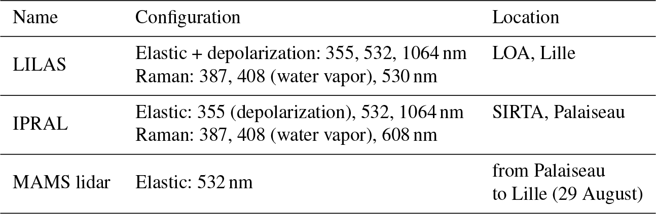
Figure 1 shows the normalized lidar range-corrected signals and columnar AOD at 532 nm derived from sun photometer measurements on 29 August 2017. The aerosol layers in the lower stratosphere, stretching from 16 to 20 km, were detected by the three lidars. The IPRAL lidar system in Palaiseau detected the aerosol layer in the range of 16–20 km on 29 August. The columnar AOD showed no significant variations, staying between 0.30 and 0.40, from 10:00 to 16:00 UTC and started decreasing from 17:00 UTC. Along the route from Palaiseau to Lille, MAMS lidar observed a layer between 16 and 20 km consisting of two well-separated layers. The columnar AOD was very stable, around 0.40, all along the route from Palaiseau to Lille. Lidar LILAS in Lille observed a shallow layer between 18 and 20 km at about 08:00 UTC on 29 August. The thickness of the layer increased to 4 km until 16:00 UTC. The columnar AOD increased from 0.20 to 0.40 from 08:00 to 14:00 UTC. The lidar quick look indicated that the aerosol content in the lower troposphere did not show significant variations during 08:00 and 12:00 UTC, so the increased optical depth, 0.2, came mainly from the contribution of the stratospheric aerosol layer.

Figure 1 Lidar range-corrected signal and columnar AOD from the sun photometer at 532 nm on 29 August 2017. (a) IPRAL system in Palaiseau. (b) MAMS lidar en route from Palaiseau to Lille. (c) LILAS in Lille. Columnar AOD measurements are interpolated from AERONET (Lille and Palaiseau) and PLASMA (mobile system) measurements. MAMS started from Palaiseau at 13:53 UTC and arrived in Lille at 16:23 UTC. The departure and arriving times are indicated in (a) and (c) with the dashed white lines.

Figure 2 shows the lidar range-corrected signal at 1064 nm on 24–25 August 2017. The plume between 17 and 18.5 km is the smoke layer. Due to cirrus clouds and low clouds in the troposphere, the lidar signals in the plume are interrupted. In the nighttime, the plume base is stable at about 17 km. Just starting from the sunrise time at 04:51 UTC, a gradual and obvious ascent is observed. In 3–4 h, the plume base ascended by about 0.6 km. Between 10:00 and 16:00 UTC, the plume base stayed stable. The ascent of smoke plume was also presented in Ansmann et al. (2018) and Khaykin et al. (2018). Khaykin et al. (2018) mentioned that the plume ascended very fast during the first few days after being injected into the troposphere. Based on the observation in Fig. 2, we derived the ascent rate of approximately 2.1–2.8 km per day, considering that the sunshine duration is 14 h (according to the latitude of Lille site) and that the vertical speed of the plume is constant. Ansmann et al. (2018) explained that the ascent of the plume may be related to the absorption of soot-containing aerosols and the wind velocity in the stratosphere. Figure 2 shows that the plume does not continuously ascend in the daytime. One possible explanation we infer is that the self-heating and the wind shear reached an equilibrium point in the plume, so it moved neither upward nor downward.

Figure 2 Lidar range-corrected signal at 1064 nm on 24–25 August 2017 measured by LILAS. The solid red line indicates the sunrise time. The two dashed red lines point out the approximate layer base before and after the sunrise. The sunrise and sunset times are 04:51 and 20:47 UTC, respectively. The corresponding daytime duration is about 14 h.

3.2 Radiosonde measurements

We take the radiosonde measurements from two stations closest to the lidar sites: Trappes (48.77^∘ N, 1.99^∘ E, France) and Beauvechain (50.78^∘ N, 4.76^∘ E, Belgium). Trappes is about 20 km from Palaiseau and Beauvechain is 120 km from Lille. Considering the large spatial distribution of the stratospheric aerosols, it is obvious that the radiosonde passed through this stratospheric smoke layer. Figure 3 shows the temperature at 00:00 and 12:00 UTC on 29 August for Trappes and 21:00 UTC on 29 August for Beauvechain. To compare, we plot the temperature profile of Trappes at 12:00 UTC on 21 August, when no stratospheric aerosol layers presented. The temperature profiles clearly show an enhancement between 16 and 20 km, which coincides with the altitude at which the stratospheric plumes appear. The spatial–temporal occurrence of this temperature enhancement and the stratosphere plume at two independent stations indicate that they are directly correlated. Fromm et al. (2005, 2008) also presented temperature increase in the stratospheric smoke layers.

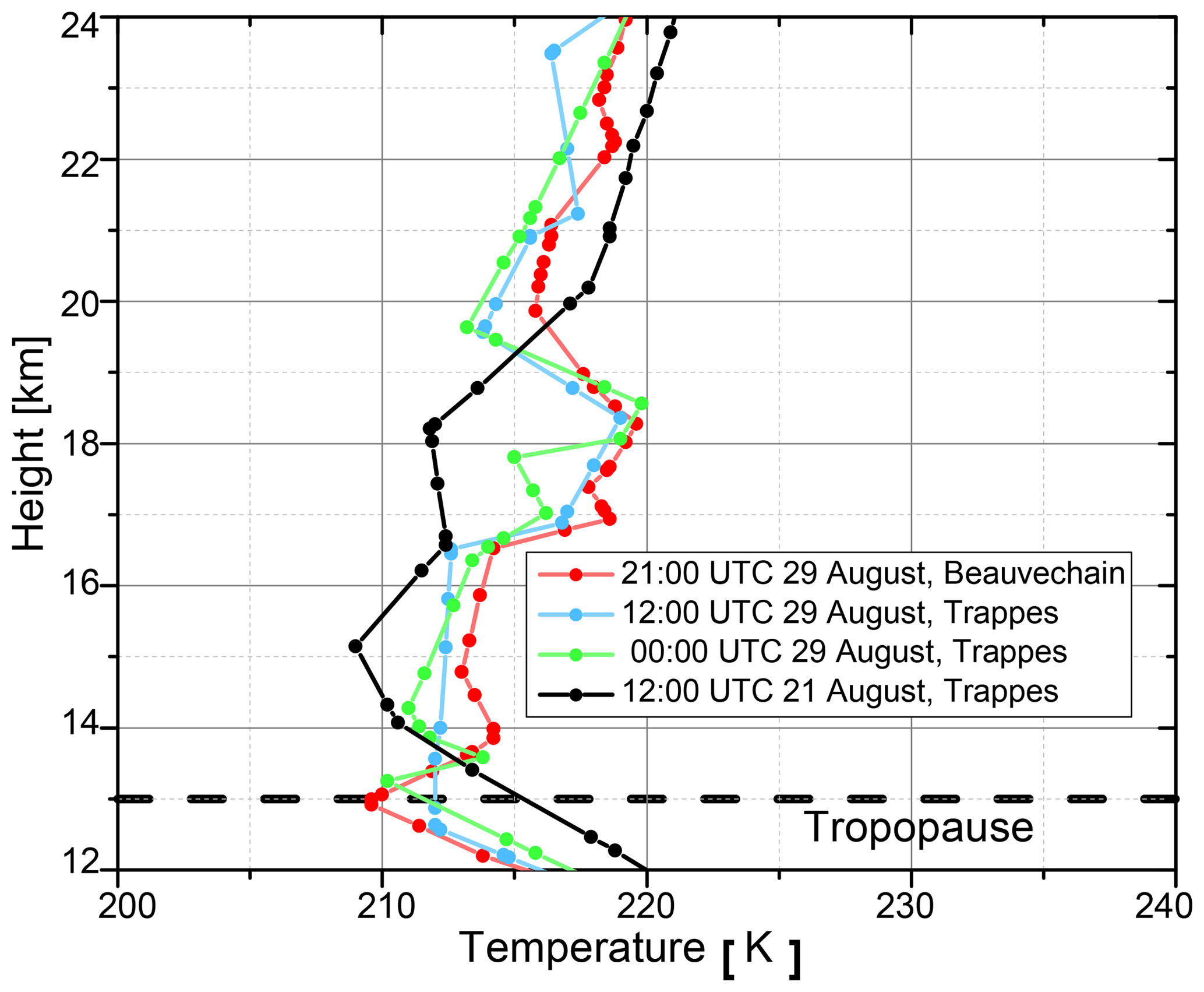
Figure 3 Temperature profiles from the radiosonde measurements. The green and cerulean lines are the temperature profiles of Trappes at 00:00 and 12:00 UTC on 29 August 2017. The red line shows the Beauvechain data at 21:00 UTC on 29 August 2017. The black line is for 12:00 UTC on 21 August in Trappes. The horizontal dashed black line at 13 km represents the approximate position of the tropopause.

3.3 MODIS measurements

MODIS is a key instrument onboard the Terra and Aqua satellites. Terra MODIS and Aqua MODIS view the entire Earth's surface every 1 to 2 days. Several episodes of Canadian wildfires have been observed by MODIS since early July 2017. On 12 August, MODIS observed a thick grey plume arising from British Columbia in the west of Canada (not shown; please see the web page of WorldView: https://worldview.earthdata.nasa.gov, last access: 15 January 2019). Figure 4 shows the Earth's true color image overlaid with the fires and thermal anomalies on 15 August 2017 when the plumes had spread over a large area. The region marked with the green dashed line is a huge visible smoke plume and in its southwest MODIS detected a belt of fire spots. Additionally, during the week of 13–19 August, MODIS (see https://worldview.earthdata.nasa.gov, last access: 15 January 2019) observed a widespread cloud coverage over Canada and showed that cloud layers were overshadowed by the smoke plumes, meaning that the plumes were lofted above the cloud layers, as shown in Fig. 4.

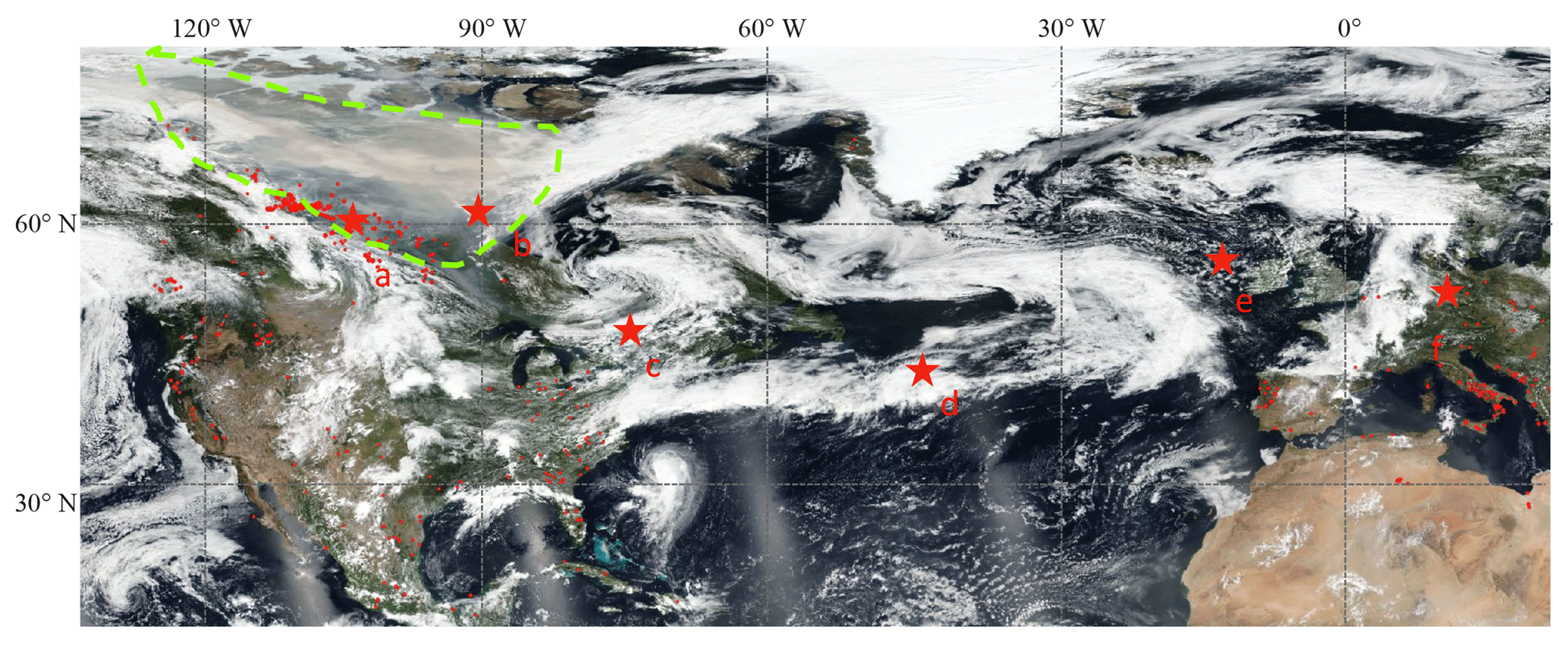
Figure 4 The corrected surface reflectance overlaid with fire and thermal anomalies from MODIS (15 August 2017). The region marked with the dashed green line in the northwest indicated a plume generated by fire activities. Six locations (labeled as red stars) on the tracks of CALIPSO are selected: (a) (61.47^∘ N, 106.44^∘ W), (b) (62.79^∘ N, 91.54^∘ W), (c) (46.97^∘ N, 72.22^∘ W), (d) (42.27^∘ N, 42.08^∘ W), (e) (55.97^∘ N, 12.54^∘ W), and (f) (52.37^∘ N, 13.47^∘ E). The corresponding overpass date is 14, 15, 17, 19, 21, and 23 August 2017.

3.4 OMPS NM UVAI maps

UVAI is a widely used parameter in characterizing UV-absorbing aerosols, such as desert dust, carbonaceous aerosols coming from anthropogenic biomass burning, wildfires, and volcanic ash. The UVAI is determined using the 340 and 380 nm wavelength channels and is defined as

$$\begin{array}{}\text{(4)}& {\displaystyle }\mathrm{UVAI}=-\mathrm{100}\times \left\{{\log }_{\mathrm{10}}{\left[{\displaystyle \frac{I_{\mathrm{340}}}{I_{\mathrm{380}}}}\right]}_{\mathrm{meas}}-{\log }_{\mathrm{10}}{\left[{\displaystyle \frac{I_{\mathrm{340}}}{I_{\mathrm{380}}}}\right]}_{\mathrm{calc}}\right\},\end{array}$$

where I₃₄₀ and I₃₈₀ are the backscattered radiance at 340 and 380 nm. The subscript “meas” represents the measurements and “calc” represents the calculation using a radiative transfer model for pure Rayleigh atmosphere. The UVAI is defined so that positive values correspond to UV-absorbing aerosols and negative values correspond to non-absorbing aerosols (Hsu et al., 1999). The OMPS NM on board the Suomi NPP (National Polar-orbiting Partnership) is designed to measure the total column ozone using backscattered UV radiation between 300 and 380 nm. A 110^∘ FOV (field-of-view) telescope enables full daily global coverage (McPeters et al., 2000; Seftor et al., 2014). Figure 5 shows the evolution of UVAI from OMPS NM (Jaross, 2017) every 2 days from 11 to 29 August 2017. The evolution of the UVAI during this event has also been shown in the study of Khaykin et al. (2018). A plume with relatively high UVAI first occurred over British Columbia on 11 August, and the intensity of the plume was moderate. An obvious increase in UVAI from 11 to 13 August was observed over the northwest of Canada. It is a clear indication that the events on 12 August were responsible for the increase in UVAI. From 13 to 17 August, the plume spread in the northwest–southeast direction and the UVAI in the center of the plume reached 10. On 19 August, the plume center reached the Labrador Sea and the forefront of the plume reached Europe. From 21 to 29 August, the UVAI in the map was much lower than the previous week. During this period, we can still distinguish a plume propagating eastward from the Atlantic to Europe, with the UVAI damping during the transport. Figure 5e–j show that Europe was overshadowed by the high-UVAI plume during 19 and 29 August.

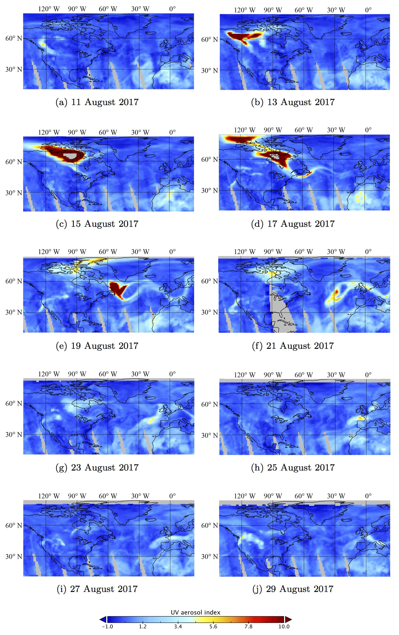
Figure 5 OMPS NM daily UVAI products from 11 to 29 August 2017. The results are plotted every 2 days. Grey indicates areas with no retrievals.

3.5 AIRS CO maps

AIRS is a continuously operating cross-track scanning sounder on board NASA's Aqua satellite launched in May 2002. AIRS covers the 3.7 to 16 µm spectral range with 2378 channels and a 13.5 km nadir FOV (Susskind et al., 2014; Kahn et al., 2014). The daily coverage of AIRS is about 70 % of the globe. AIRS is designed to measure the water vapor and temperature profiles. It includes the spectral features of the key carbon trace gases, CO₂, CH₄, and CO (Haskins and Kaplan, 1992). The current CO product from AIRS is very mature because the spectral signature is strong and the interference of water vapor is relatively low (McMillan et al., 2005). CO, as a product of the burning process, can be taken as a tracer of biomass burning aerosols (Andreae et al., 1988) due to its relatively long lifetime of 0.5 to 3 months. CO can also originate from anthropogenic sources, for example engines of vehicles (Vallero, 2014). In August 2017, the wildfire activities were so intense that the CO plumes rising from the fire region were much more significant than the background. This strong contrast makes CO a good tracer for the transport of the smoke plumes.

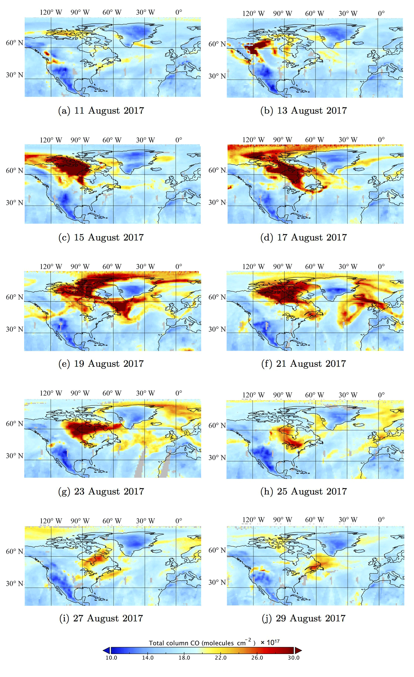
Figure 6 Total CO concentration (molecules cm⁻²) retrieved from AIRS. The maps are plotted every 2 days from 11 to 29 August 2017.

Figure 6 shows the evolution of the total column CO concentration (Texeira, 2013) every 2 days during the period of 11 to 29 August 2017. CO concentration strongly increased in the west and north of Canada from 11 to 13 August, similar to the UVAI shown in Fig. 5. The forefront of the CO plume reached the west and north of Europe since 19 August. We find that the spatial distribution and temporal evolution of CO are strongly co-related with the UVAI. This correlation is very evident before 21 August. After 21 August, the correlation became weaker, for the UVAI in North America was decreasing fast while the CO concentration remained almost unchanged or decreased much more slowly. This is possibly due to the longer lifetime of CO compared to UVAI. Combing the MODIS image and the UVAI and CO spatial–temporal evolution, we conclude that the aerosol plumes observed in Europe were smoke transported from Canada.

3.6 CALIPSO measurements

CALIPSO measurements provide a good opportunity to investigate the vertical structure of the plumes and trace back the transport of the plumes. CALIPSO measures the backscattered signal at 532 and 1064 nm. One parallel channel and one perpendicular channel are coupled to derive the particle linear depolarization ratio at 532 nm. Figure 7a–f present the profiles of the backscatter coefficient and particle linear depolarization ratio at 532 nm, corresponding to the six locations a–f in Fig. 4. These data were obtained from the NASA Langley Research Center Atmospheric Science Data Center. The six locations are intentionally selected, falling in the region with elevated UVAI and CO concentration and following the transport pathway of the plume (in Figs. 5 and 6) from Canada to Europe. Figure 7 shows the enhancements of backscatter in the upper troposphere and lower stratosphere. Aerosol and cloud are both possible causes of the backscatter enhancements and can be distinguished by using the particle depolarization ratio. We have examined the temperature profiles over several sites in North America in August 2017 and found that, above 10 km, the temperature drops below −38 ^∘C; at this temperature clouds consist mainly of ice crystals. The particle depolarization ratio is usually no less than 0.40 for ice cloud and from a few percent to about 0.40 for mixed-phase cloud.

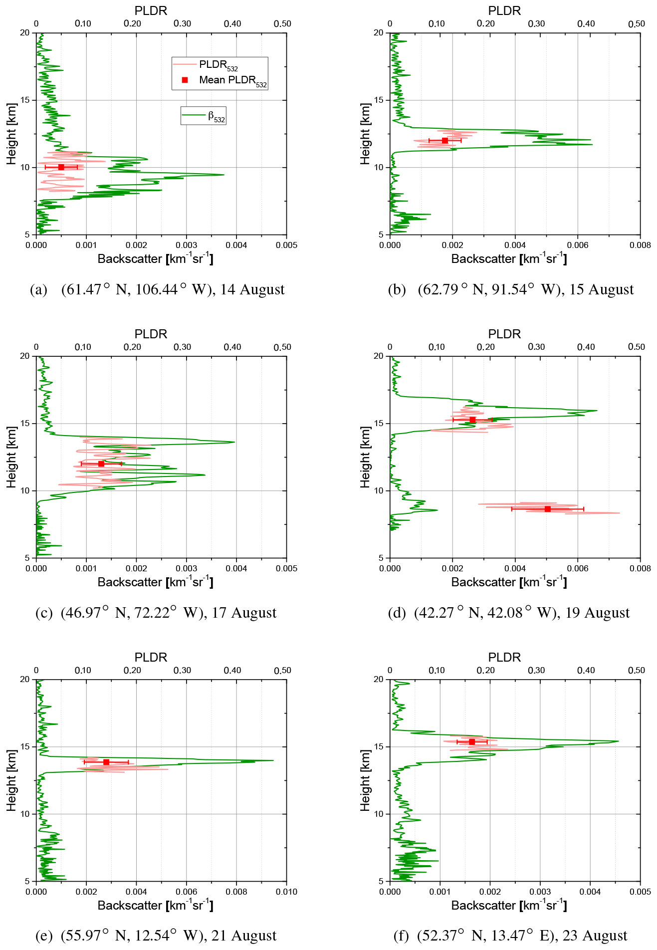
Figure 7 The profiles of backscatter coefficient and particle linear depolarization ratio (PLDR) at 532 nm from CALIPSO. Panels (a)–(f) correspond to the six locations (a)–(f) in Fig. 4. The corresponding CALIPSO tracks are (a) 09:50:19, 14 August 2017; (b) 08:54:37, 15 August 2017; (c) 07:03:13, 17 August 2017; (d) 06:50:44, 19 August 2017; (e) 03:20:25, 21 August 2017; and (f) 01:29:01, 23 August 2017. A total of 20 profiles are averaged over these six locations. The solid green and pink lines represent backscatter coefficient and particle linear depolarization ratio, respectively. The red squares with error bars represent the mean particle linear depolarization ratio and the standard deviation within each layer.

Figure 7a and b show the aerosol layers observed on 14 and 15 August over the north of Canada; both locations lay in the area where MODIS observed a smoke plume on 15 August (Fig. 4) and the area with high UVAI and CO concentration. The particle linear depolarization ratio is about 0.05 in Fig. 7a and 0.10 in Fig. 7b, meaning that it is an aerosol layer instead of ice or mixed-phase cloud. Figure 7c and f show stratospheric layers detected at 10–20 km in height, with the depolarization varying from 0.10 to 0.18. The lower layer at about 9 km in Fig. 7d has a depolarization ratio between 0.20 and 0.45 (median 0.32), which falls into the category of ice or mixed-phase clouds. Profiles in Fig. 7f were captured over Berlin at 01:29 UTC on 23 August. About 150 km to the southwest, a lidar in Leipzig measured stratospheric smoke layers (Haarig et al., 2018). The particle depolarization ratio of CALIPSO at 532 nm on 23 August is consistent with ground-based lidar measurements in Lille and Leipzig, which will be presented in Sect. 4. It should be noted that aerosol types of the plumes in Fig. 7 are quite uncertain in the CALIPSO product. These layers are classified into scattered aerosol types, such as polluted dust, elevated smoke, and volcanic ash. This misclassification could introduce some extent of errors to the backscatter profile and particle depolarization profiles.

4 Results and analysis

4.1 Overview of retrieved optical parameters

We selected and averaged the lidar measurements in 10 time intervals, among which five periods are from the LILAS system in Lille: 22:00 (24 August)–00:30 UTC (25 August); 13:00–16:00 UTC, 16:00–18:00 UTC (29 August); 20:00–23:00 UTC (31 August); and 23:00 (31 August)–02:00 UTC (1 September); two intervals are from the IPRAL system in Palaiseau: 16:00–18:00 and 19:20–21:20 UTC (28 August). Three intervals are from the mobile lidar in the MAMS system (29 August): 14:00–15:00 UTC (corresponding spatially to a 100 km distance from Palaiseau to Compiègne), 15:00–15:45 UTC (100 km on the route from Compiègne to Arras), and 16:15–16:30 UTC at Lille.

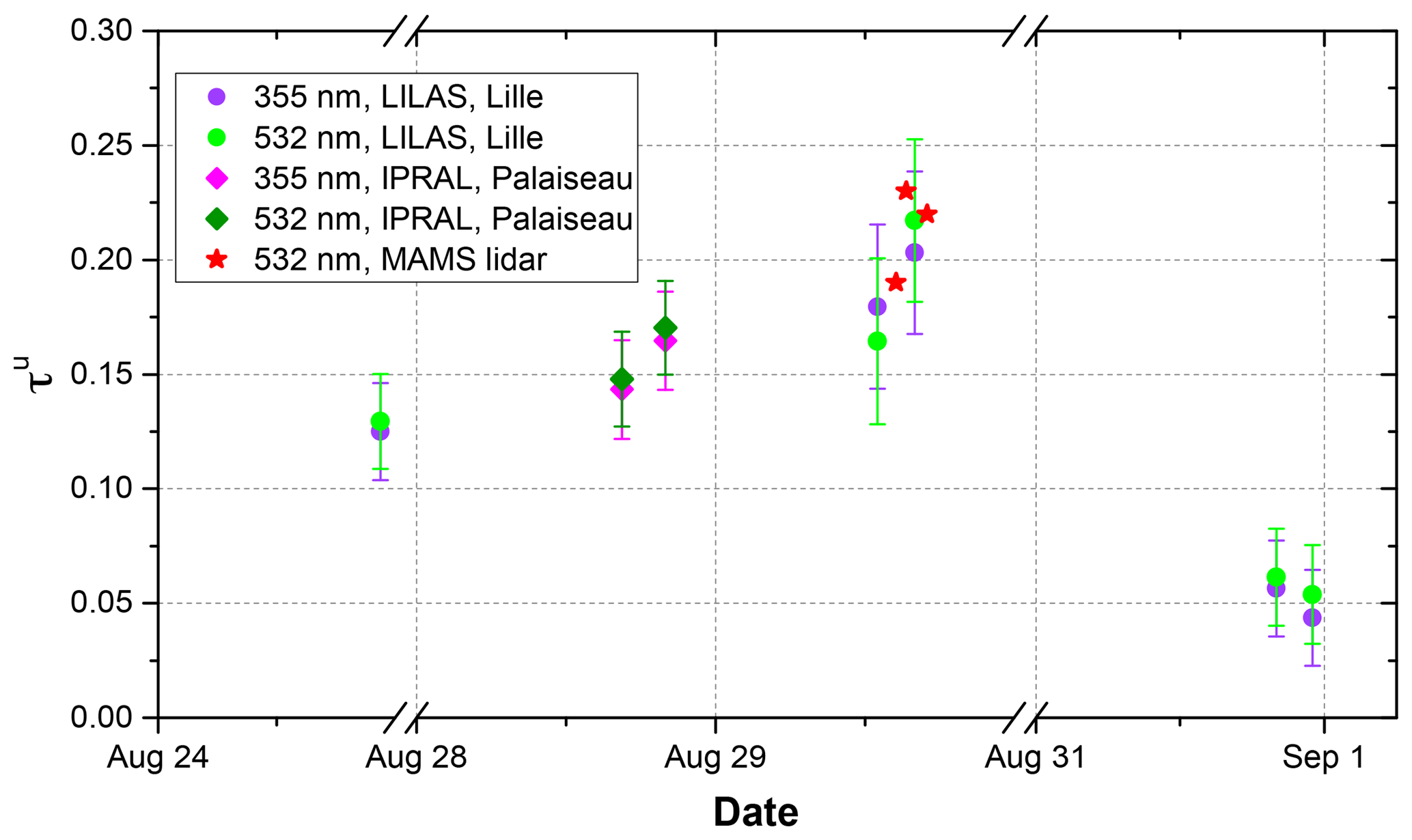
Figure 8 Optical depth of the stratospheric smoke layer at 355 and 532 nm estimated from lidar signals in August 2017. The optical depth estimated from LILAS (in Lille) is plotted with solid green (532 nm) and violet circles (355 nm). Optical depth calculated from IPRAL (in Palaiseau) is plotted with solid dark green (532 nm) and magenta (355 nm) diamonds. The red stars represent the optical depth calculated from the MAMS lidar.

Figure 8 shows the optical depth of the stratospheric layer varying from 0.05 to 0.23 (at 532 nm). The spectral dependence of the optical depth of 355 and 532 nm is very weak. The maximal optical depth of the stratospheric layer was observed in the afternoon of 29 August, between 16:00 and 18:00 UTC. The LILAS system observed AOD of 0.20±0.04 at 355 nm and 0.21±0.04 at 532 nm. As discussed in Sect. 3.1, the columnar AOD at 532 nm from AERONET increased by about 0.20 after the presence of the stratospheric layer, which agrees well with the derived optical depth of the stratospheric layer. The minimum of the optical depth appeared in the night of 31 August 2017, giving 0.04±0.02 at 355 nm and 0.05±0.02 at 532 nm. The optical depth of the stratospheric layer along the route, observed by MAMS, is as follows: 0.19 over a distance of 100 km north from Palaiseau, 0.23 along 100 km of the middle of the transect from Compiègne to Arras, and 0.22 when arriving at Lille.

Due to the insufficient signal-to-noise ratio above the stratospheric plume, the MAMS lidar measurements are processed using the Klett method and constrained by the columnar AOD measured by the PLASMA sun photometer. Klett inversion is performed on the lidar profile from the surface to the top of the stratospheric layer, assuming a vertically independent lidar ratio. The optical depth of the stratospheric smoke layer is then calculated from the integral of the extinction profile. As a result, the error of the estimated smoke optical depth from MAMS measurements is difficult to quantify. Here we present the optical depth from MAMS lidar for a comparison.

Table 2 Retrieved lidar ratios (LRs), particle linear depolarization ratios (PLDRs), layer thickness, and mean extinction coefficients from multi-wavelength lidar systems LILAS in Lille and IPRAL in Palaiseau. $\overline{\mathit{\alpha }}$ is the mean extinction coefficient in the stratospheric smoke layer. ΔL is the thickness of the stratospheric smoke layer. The values after “±” represent the errors. Error estimation is presented in the Appendix.

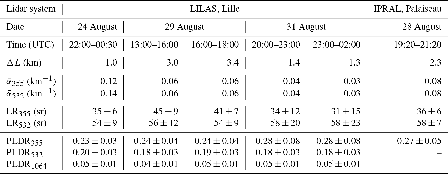
Table 2 summarizes the lidar ratio and particle depolarization ratio in the stratospheric aerosol layer. Lidar ratios vary between 54±9 and 58±23 sr at 532 nm and between 31±15 and 45±9 sr at 355 nm. The results from two different lidar systems and with different observation times agree well, indicating that the properties of the stratospheric layer are spatially and temporally stable. We derived a higher lidar ratio at 532 than at 355 nm, which is a characteristic feature of aged smoke and has been observed in previous studies (Wandinger et al., 2002; Murayama et al., 2004; Müller et al., 2005; Sugimoto et al., 2010). In the night of 31 August, the error of lidar ratio is about 30 %–35 %, relatively higher than the other days because of the low optical depth. Although the error varies, the mean values of derived lidar ratios are relatively stable. The particle depolarization ratio decreases as wavelength increases. At 1064 nm, the particle linear depolarization ratio is very stable, varying from 0.04±0.01 to 0.05±0.01. At 532 nm, the particle linear depolarization ratio is also stable, varying from 0.18±0.03 to 0.20±0.03. The particle linear depolarization ratio at 355 nm increased from 0.23±0.03 on 24 August to 0.28±0.08 on 31 August. However, the increase is within the range of the uncertainties. The particle depolarization ratio at 532 nm is in good agreement with CALIPSO observations shown in Fig. 7c–f. The particle depolarization ratio at 355 nm measured by LILAS is consistent with the IPRAL system. Haarig et al. (2018) measured 0.23 at 355 nm, 0.18 at 532 nm, and 0.04 at 1064 nm in the stratospheric smoke layers on 22 August 2017, showing excellent agreements with our study.

The errors of particle depolarization ratio are calculated with the method in the Appendix. The estimated errors of the particle depolarization ratio are generally below 15 %, except the 355 nm channel in the night of 31 August when the optical depth was the lowest in all the investigated observations in this study. On 31 August, the backscatter ratio, volume depolarization ratio, and molecular depolarization ratio at 355 nm are approximately: 3.5 (50 %), 0.15 (10 %), and 0.004 (200 %). The values in the parentheses are the relative errors of the quantity on their left. The resulting error of particle depolarization is about 28 %. At 532 nm, we derive 12 % of error for the particle depolarization ratio when the backscatter ratio, volume depolarization ratio, and molecular depolarization ratio are 10 (50 %), 0.15 (10 %), and 0.004 (200 %). In the same way, we derive less than 11 % of error for the particle depolarization ratio at 1064 nm. The error at 355 nm is estimated to be higher than 532 and 1064 nm as the interferences of molecular scattering are stronger at this channel. When the layer is optically thicker, for example, on 24 August, the error of 355 nm is estimated to be less than 13 %. Conservatively, we use 30 % for the error of the particle linear depolarization ratio at 355 nm on 31 August and 15 % for the error of the rest.

4.2 Case study

4.2.1 Optical properties

We select the night measurements of 24 August in Lille and 28 August in Palaiseau as two examples. The two systems were operating independently, so that the results from two different systems that measured at different times can be regarded as verifications for each other.

Figure 9 (a) Extinction and backscatter coefficients, (b) particle linear depolarization ratio (PLDR), and the extinction-related Ångström exponent (EAE) and backscatter-related Ångström exponent (BAE) retrieved from LILAS observations between 22:00 UTC on 24 August 2017 and 00:30 UTC on 25 August 2017 at Lille. The errors of extinction, backscatter coefficient, and corresponding Ångström exponent at 355 and 532 nm are attributed to the error of the optical depth.

24 August 2017, Lille

Figure 9 shows the retrieved optical properties of the stratospheric smoke layer observed by the LILAS system in the night of 24 August in Lille. The stratospheric aerosol layer is between 17 and 18 km, and we retrieved the extinction and backscatter profiles by assuming that the lidar ratios are 36 sr at 355 nm and 54 sr at 532 nm. The lidar ratio at 1064 nm is assumed to be 60 sr. The extinction coefficient within the layer is about 0.12–0.22 km⁻¹ at 355 and 532 nm. It should be noted that the profile of the extinction coefficient is similar to the backscatter coefficient profile because we assume the aerosol lidar ratio is vertically constant within the smoke layer. A comparison of backscatter coefficient profile has been made (not shown) between Klett and Raman methods. We found that the difference of the backscatter coefficient profiles from the two methods is very minor, indicating that our results are reliable. Assuming a vertically constant aerosol lidar ratio in the smoke layer is not unrealistic, as one can see that the particle linear depolarization ratios in the smoke layer have no noticeable vertical variation, indicating that the smoke particles are well mixed. The extinction-related Ångström exponent for 355 and 532 nm is around 0.0±0.5; the backscatter-related Ångström exponent at corresponding wavelengths is about 1.0±0.5. The particle depolarization ratios decrease as wavelength increases: 0.23±0.03 at 355 nm, 0.20±0.03 at 532 nm, and 0.05±0.01 at 1064 nm. No parameters in Fig. 9b exhibit noticeable vertical variations.

28 August 2017, Palaiseau

Figure 10 shows the retrieved optical parameters from IPRAL observations at 19:20–21:20 UTC on 28 August 2017 in Palaiseau. The thickness of the stratospheric layer is about 2.3 km, spreading from 17.2 to 19.5 km. Klett inversion was applied with an estimated lidar ratio of 36 sr at 355 nm and 58 sr at 532 nm. At 1064 nm the lidar ratio was assumed to be 60 sr. The maximum extinction coefficient in the layer reached 0.12 km⁻¹ at 532 nm. The extinction-related Ångström exponent between 355 and 532 nm is about $-\mathrm{0.06}\pm \mathrm{0.5}$. The corresponding backscatter Ångström exponent is about 1.2±0.5. The particle linear depolarization ratio at 355 nm is about 0.27±0.05. The particle linear depolarization ratio at 355 nm and extinction and backscatter-related Ångström exponents between 355 and 532 nm do not show evident vertical variations.

Figure 10 (a) Extinction and backscatter coefficients, (b) the particle linear depolarization ratio (PLDR) at 355 nm, and the extinction-related Ångström exponent (EAE) and backscatter-related Ångström exponent (BAE) (between 355 and 532 nm) retrieved from IPRAL observations between 19:20 and 21:20 UTC on 28 August 2017 in Palaiseau.

4.2.2 Microphysical properties

A regularization algorithm is applied to the vertically averaged extinction coefficients (at 355 and 532 nm) and backscatter coefficients (at 355, 532, and 1064 nm) in Figs. 9 and 10. Treating nonspherical particles is a challenging task. Many studies have been performed to model the light scattering of nonspherical particles. The spheroid model was used to retrieved dust properties (Dubovik et al., 2006; Mishchenko et al., 1997; Veselovskii et al., 2010). Both sphere and spheroid models are used to retrieve particle microphysical properties in our study. The retrievals using sphere and spheroid models are rather consistent except the imaginary part of the refractive index. The spheroid model tends to underestimate the imaginary part of the complex refractive indices, if the measured particle depolarization ratios are used. This demonstrates the deficiency of the spheroid mode in retrieving highly-absorbent and irregular-shaped smoke particles. The size of smoke particles is expected to be not very big so that a sphere model should be able to provide reasonable results. The particle linear depolarization ratio is not used in the retrieval, and the spectral dependence of complex refractive indices is also ignored. The derived effective radius (R_eff), volume concentration (V_c), and real (m_R) and imaginary (m_I) parts of the refractive indices are summarized in Table 3.

Table 3 Retrieved microphysical properties using the lidar data in Lille and Palaiseau. Extinction and backscatter coefficients shown in Figs. 9a and 10a are averaged in the range of 17–18.0 and 17.5–19.5 km, respectively. The averaged extinction and backscatter coefficients are used as the input of the regularization algorithm to retrieve particle microphysical properties.

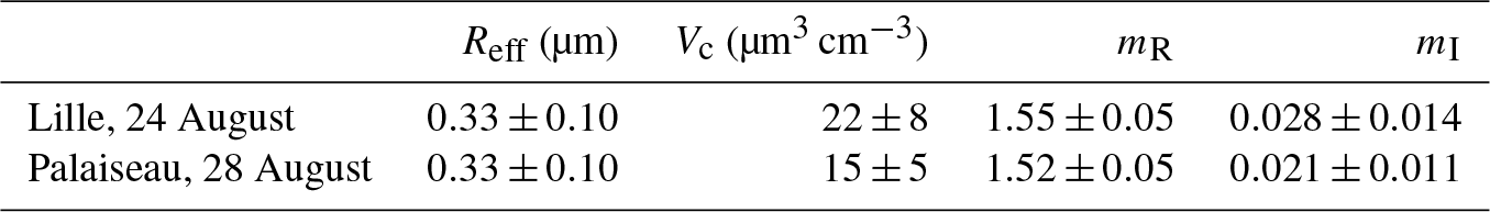
The retrieved particle size distributes in the range of 0.1 to 1.0 µm, with an effective radius (volume-weighted sphere radius) of 0.33±0.10 for both Palaiseau data and Lille data. The volume concentration is 15±5 µm³ cm⁻³ for Palaiseau data and 22±8 µm⁻³ cm³ for Lille data. The complex refractive indices retrieved from Lille and Palaiseau data are also in good agreement, giving 1.55±0.05 and 1.52±0.05 for the real part and 0.028±0.014 and 0.021±0.010 for the imaginary part. The single-scattering albedos are estimated to be 0.82–0.89 for Lille data and 0.86–0.90 for Palaiseau data. The derived aerosol microphysical properties from Palaiseau and Lille data are consistent.

The errors of the retrieved parameters have been discussed in the relevant papers (Müller et al., 1999; Veselovskii et al., 2002; Pérez-Ramírez et al., 2013). About 30 % of relative error is derived for the effective radius and volume concentration, ±0.05 (absolute value) is expected for the real part of refractive indices, and 50 % is derived for the imaginary part of refractive radius. In our case, one significant limitation is that using a sphere model does not allow us to reproduce the particle depolarization ratios. We input the retrieved size distribution (not shown) and complex refractive indices in Table 3 into the spheroid model, and we found that the spheroid model (85 % spheroid and 15 % sphere) can reproduce the spectral depolarization ratios with satisfactory accuracy: 0.21, 0.19, and 0.07 at 355, 532, and 1064 nm, respectively. However, the argument is not enough to justify that the aforementioned uncertainty estimation from previous researchers is also applicable to our retrievals. We provide this estimate as a reference, but at the current stage, we are not able to provide more quantitative and accurate error estimation for the retrieved microphysical properties.

4.2.3 Direct radiative forcing effect

The stratospheric plumes observed on 24 and 28 August in Lille and Palaiseau are optically thick, with an extinction coefficient about 10 times higher than in the volcanic ash observed by Ansmann et al. (1997) in April 1992, 10 months after the eruption of Mount Pinatubo. The radiative forcing imposed by the observed layers poses a curious question. We input the retrieved microphysical properties into GARRLiC/GRASP to estimate the DRF effect of the stratospheric plumes in Lille and Palaiseau. We assume the vertical volume concentration of aerosols follows the extinction profile in Figs. 9 and 10. The surface BRDF parameters for Lille and Palaiseau are taken from AERONET. The upward and downward flux and efficiencies as well as the net DRF (ΔF, with respect to a pure Rayleigh atmosphere) of the stratospheric aerosol layers are calculated and Table 4 shows the daily averaged net DRF (W m⁻²) at four levels: at the bottom of the atmosphere (BOA), below the stratospheric layer, above the stratospheric layer, and at the top of the atmosphere (TOA). For the layer observed in Lille on 24 August, the top and base of the stratosphere are selected as 18.4 and 16.7 km and for Palaiseau observations they are 20 and 17.0 km.

Table 4 Daily averaged net DRF flux calculated by GARRLiC/GRASP. Aerosol microphysical properties in Table 3 and aerosol vertical distributions in Figs. 9a and 10a are used to calculate the DRF effect at the following four vertical levels.

At the TOA, the net DRF flux is estimated to be −1.2 and −3.5 W m⁻² for Lille and Palaiseau data, respectively. The corresponding forcing efficiencies are −7.9 and −21.5 W m⁻² τ⁻¹. At the BOA, the net DRF flux is estimated to be −12.3 W m⁻² for Lille data and −14.5 W m⁻² for Palaiseau data. The corresponding forcing efficiencies are −79.6 and −89.6 W m⁻² τ⁻¹. We noticed that the difference in net DRF flux between the layer top and layer base is significant. For Lille data, we obtained 9.9 W m⁻² of difference between the top and the base of the stratospheric layer and for Palaiseau, we obtained 11.1 W m⁻². Because of the high imaginary part of the refractive indices, the stratospheric aerosols have the capacity of absorbing the incoming radiation, thus reducing the upward radiation at the top of the stratospheric layer and the downward radiation at the base of the stratospheric aerosol layer. The heating rate of the stratospheric layer is estimated to be 3.3 K day⁻¹ for Palaiseau data and 3.7 K day⁻¹ for Lille data. This qualitatively explains the increase in temperature within the stratospheric layer, as observed by the radiosonde measurements shown in Fig. 3. Due to high uncertainty in the retrieved particle microphysical properties, the uncertainty of the calculated DRF could be large.

5 Discussion

The measurements revealed high particle depolarization ratios in the stratospheric smoke at 355 and 532 nm. In particular, the particle depolarization ratio at 355 nm ranges from 0.23±0.03 to 0.28±0.08, while at 532 nm it is about 0.19±0.03. The depolarization ratio at 1064 nm is significantly lower, about 0.05±0.01. Similar spectral dependences of depolarization ratios, 0.20, 0.09, and 0.02 at 355, 532, and 1064 nm, respectively, were observed by Burton et al. (2015) in a smoke plume at 7–8 km in altitude (on 17 July 2014) in North American wildfires. Particle depolarization ratios of 0.07 and 0.02 at 532 and 1064 nm, respectively, were observed in a Canadian smoke plume at 6 km (on 2 August 2007) over the US (Burton et al., 2012). In Burton et al. (2012) and Burton et al. (2015), the smoke traveled approximately 3 days and 6 days, respectively. The travel times in both cases are shorter than in our study. The light-scattering process leading to high particle depolarization ratios of smoke particles has not been revealed yet. In previous studies, smoke mixed with soil particles was suggested to be the explanation (Fiebig et al., 2002; Murayama et al., 2004; Müller et al., 2007a; Sugimoto et al., 2010; Burton et al., 2012, 2015; Haarig et al., 2018). Strong convections occurring in fire activities in principle are capable of lifting soil particles into the smoke plume (Sugimoto et al., 2010).

A high depolarization ratio with similar spectral dependence has been observed in fine dust particles. Miffre et al. (2016) measured the particle depolarization ratio of two Arizona Test Dust samples at backscattering angle. The radii of the dust samples are mainly below 1 µm. They obtained a higher depolarization ratio at 355 nm than at 532 nm, and the depolarization ratios at both wavelengths are over 0.30. The sharp edges and corners in the artificial dust samples are a possible reason for the measured high particle depolarization ratio. In the study of Järvinen et al. (2016), over 200 dust samples were used to measure the near-backscattering (178^∘) properties and it is found that, for fine-mode dust, the particle depolarization ratio has a strong size dependence. Järvinen et al. (2016) obtained about 0.12–0.20 and 0.25–0.30 for the depolarization ratio for equivalent particle size parameters at 355 and 532 nm. Sakai et al. (2010) measured the depolarization of Asian and Saharan dust in the backscattering direction and obtained 0.14–0.17 at 532 nm for the samples with only sub-micrometer particles and 0.39 for the samples with high concentrations of super-micrometer particles. Mamouri and Ansmann (2017) concluded that the depolarization spectrum of fine dust is 0.21±0.02 at 355 nm, 0.16±0.02 at 532 nm, and 0.09±0.02 at 1064 nm. This spectrum is very similar to the Canadian stratospheric smoke aerosol presented in this study and Haarig et al. (2018).

However, Murayama et al. (2004) suggested that the coagulation of smoke particles to the clusters with complicated morphology is a more reasonable explanation because they found no signature of mineral dust after analyzing the chemical compositions of the smoke sample. Mishchenko et al. (2016) modeled the spectral depolarization ratios observed by Burton et al. (2015) and found that such behavior results from complicated morphology of smoke particles. Kahnert et al. (2012) modeled the optical properties of light-absorbing carbon aggregates (LACs) embedded in a sulfate shell. It was found that the particle depolarization ratio increases with the aggregate radius (volume-equivalent sphere radius). For the case of 0.4 µm aggregate radius and 20 % LAC volume fraction, the computed depolarization ratios are 0.12–0.20 at 304.0 nm, 0.08–0.18 at 533.1 nm, and about 0.015 at 1010.1 nm, which are comparable with the results in this study and Haarig et al. (2018). In this study, we are not able to assess which is the dominant factor leading to the high depolarization ratios, possibly both the soil particles and smoke aging process are partially responsible.

The derived lidar ratios are from 31±15 to 45±9 sr for 355 nm and from 54±12 to 58±23 sr for 532 nm. Considering the uncertainties of the lidar ratio, the derived values and the spectral dependence agree well with previous publications (Müller et al., 2005; Sugimoto et al., 2010; Haarig et al., 2018) about aged smoke observations. Haarig et al. (2018) obtained about 40 sr at 355 nm and 66 sr at 532 nm, using the Raman method. The retrieved effective radius is about 0.33±0.10 µm, consistent with the particle size obtained by Haarig et al. (2018). The particle size is larger than the values of fresh smoke observed near the fire source (O'Neill et al., 2002; Nicolae et al., 2013). In particular, the retrieved particle size agrees well with the observed smoke transported from Canada to Europe (Wandinger et al., 2002; Müller et al., 2005). Müller et al. (2007b) found that the effective radius increased from 0.15–0.25 µm (2–4 days after the emission) to 0.3–0.4 µm after 10–20 days of transport time, which is consistent with our results. But it is worth noting that Müller et al. (2007b) investigated only tropospheric smoke and it is not clear if this effect of the aging process is applicable to stratospheric smoke.

The real part of the refractive indices obtained in this study is 1.52±0.05 for Palaiseau data and 1.55±0.05 for Lille data, without considering the spectral dependence. The values are consistent with the results for tropospheric smoke (Dubovik et al., 2002; Wandinger et al., 2002; Taubman et al., 2004; Müller et al., 2005). As for the imaginary part, we derived 0.021±0.010 from Palaiseau data and 0.028±0.014 from Lille data. The imaginary part of refractive indices of smoke in previous studies is diverse. Müller et al. (2005) reported the imaginary part varying around 0.003 for non-absorbing tropospheric smoke originating from aged Siberian and Canadian forest fires. Wandinger et al. (2002) obtained 0.05–0.07 for the imaginary part of Canadian smoke in the troposphere over Europe. Dubovik et al. (2002) derived about 0.01 to 0.03 for the imaginary part of biomass burning using photometer observations. The retrieved imaginary part in our study falls into the range of previously reported values. Using a sphere model in the inversion is potentially an important error source, as spheres cannot fully represent the scattering of irregular aged smoke particles. The application on dust particles (Veselovskii et al., 2010) demonstrated that retrieved volume concentration and effective radius are still reliable and the main error is attributed to the imaginary part of the refractive index. Errors in the optical data are also a potential error source of the retrieved microphysical parameters.

The relative humidity in the smoke layer is one factor that impacts the refractive indices, the particle depolarization ratio, and lidar ratio of smoke particles. However, in some studies, the relative humidity is not mentioned, thus making the comparison difficult. Special attention should be paid to the relative humidity when comparing the complex refractive indices. Mixing with other aerosol types during transport is also a potential cause of the modification of aerosol properties, and its impact is not limited to the refractive indices. In this study, the smoke layers we observed were lofted to the lower stratosphere in the source region and then transported to the observation sites. They were isolated from other tropospheric aerosol sources and not likely to mix with them during the transport. The relative humidity in the stratospheric layer was below 10 %, according to the radiosonde measurements. Our study provides a reference for aged smoke aerosols in a dry condition.

The retrieved particle parameters allow an estimation of direct aerosol radiative forcing. We derived −79.6 W m${}^{-\mathrm{2}}{\mathit{\tau }}^{-\mathrm{1}}$ for the DRF efficiency at the BOA for Lille data. And for Palaiseau data, we derived −89.6 W m${}^{-\mathrm{2}}{\mathit{\tau }}^{-\mathrm{1}}$. This indicates that the observed stratospheric aerosol layers strongly reduce the radiation reaching the terrestrial surface mainly by absorbing solar radiation. Derimian et al. (2016) evaluated the radiative effect of several aerosol models, among which the daily net DRF efficiency of biomass burning aerosols is estimated to be −74 to −54 W m${}^{-\mathrm{2}}{\mathit{\tau }}^{-\mathrm{1}}$ at the BOA. Mallet et al. (2008) studied the radiative forcing of smoke and dust mixtures over Djougou and derived −68 to −50 W m${}^{-\mathrm{2}}{\mathit{\tau }}^{-\mathrm{1}}$ for the DRF efficiency at the BOA. Our results are comparable with the values in the publications. Additionally, the mean heating rate of the stratospheric smoke layer is estimated to be about 3.5 K day⁻¹ for Lille and for Palaiseau data, which qualitatively supports the temperature increase within the stratospheric smoke layer. The warming effect in the layer is potentially responsible for the upward movements of soot-containing aerosol plumes (Laat et al., 2012; Ansmann et al., 2018). The high uncertainty in the retrieved microphysical properties, especially the imaginary part of the refractive indices, will propagate into the DRF estimation. At the current stage, we are not able to accurately estimate the uncertainty in the microphysical properties and in the DRF calculation. Varying the imaginary part by ±50 %, we calculated the variability in the DRF efficiency at the BOA and the heating rate, and we derived about 20 % variation in the DRF efficiency at the BOA and 40 % variation in the heating rate.

6 Conclusion

In the summer of 2017, large-scale wildfires spread in the west and north of Canada. The severe fire activities generated strong convections that lofted smoke plumes up to the high altitudes. After long-range transport, the smoke plumes spread over large areas. Three lidar systems in northern France observed aged smoke plumes in the stratosphere, about 10–17 days after the intense fire emissions in mid-August. Unlike fresh smoke particles, the aged smoke particles showed surprisingly high particle depolarization ratios, indicating the presence of irregular smoke particles. Lidar data inversion revealed that the smoke particles are relatively bigger compared to fresh smoke particles and very absorbent. The strong absorption of the observed smoke plumes is related to the perturbation of the temperature profile and the ascent of the plume when exposed to sunlight. In addition, the DRF estimation indicated that the stratospheric smoke can strongly reduce the radiation reaching the bottom of the atmosphere.

This study shows the capability of multi-wavelength Raman lidar in aerosol profiling and characterization. We reported important optical and microphysical properties derived from lidar observations; these results help to improve our knowledge about smoke particles and aerosol classification, which is an important topic in the lidar community. Future improvements in better quantifying the uncertainty in the optical and microphysical properties are highly anticipated. Moreover, this event is also a good opportunity for the study of the atmospheric model. The injection of smoke into the upper troposphere and lower stratosphere by strong convection needs to be considered in atmospheric models. The self-lifting of absorbing smoke is not yet considered in any aerosol transport model. Additionally, this event provides a favorable chance for studying smoke aging processes, the smoke plumes stayed in the stratosphere more than 1 month and were observed by ground-based lidars and CALIPSO. Much more effort is needed in investigating these measurements.

Appendix A: Error estimation

A1 Errors of optical depth

The errors in the lidar signal at the top and the base of the stratospheric layers are considered to be the major error sources in the error estimation of the optical depth. We estimate the error of the lidar signal $\stackrel{\mathrm{‾}}{P}(\mathit{\lambda },r_{\mathrm{top}})$ and $\stackrel{\mathrm{‾}}{P}(\mathit{\lambda },r_{\mathrm{base}})$ to be 3 %–5 %, based on the statistical error of photon distributions. According to Eq. (2), the error of the optical depth, $\frac{\mathrm{\Delta }{\mathit{\tau }}^u}{{\mathit{\tau }}^u}$, is written as

$$\begin{array}{ll}{\displaystyle }{\left({\displaystyle \frac{\mathrm{\Delta }{\mathit{\tau }}^u}{{\mathit{\tau }}^u}}\right)}^{\mathrm{2}}& {\displaystyle }=F_{{\stackrel{\mathrm{‾}}{P}}_{\mathrm{top}}}{\left({\displaystyle \frac{\mathrm{\Delta }\stackrel{\mathrm{‾}}{P}(\mathit{\lambda },r_{\mathrm{top}})}{\stackrel{\mathrm{‾}}{P}(\mathit{\lambda },r_{\mathrm{top}})}}\right)}^{\mathrm{2}}\\ \text{(A1)}& {\displaystyle }& {\displaystyle }+F_{{\stackrel{\mathrm{‾}}{P}}_{\mathrm{base}}}{\left({\displaystyle \frac{\mathrm{\Delta }\stackrel{\mathrm{‾}}{P}(\mathit{\lambda },r_{\mathrm{base}})}{\stackrel{\mathrm{‾}}{P}(\mathit{\lambda },r_{\mathrm{base}})}}\right)}^{\mathrm{2}},\end{array}$$

$$\begin{array}{}\text{(A2)}& {\displaystyle }{\displaystyle }{F}_{{\stackrel{\mathrm{‾}}{P}}_{\mathrm{top},\mathrm{base}}}={\left({\displaystyle \frac{\stackrel{\mathrm{‾}}{P}(\mathit{\lambda },r_{\mathrm{top},\mathrm{base}})}{{\mathit{\tau }}^u}}{\displaystyle \frac{\partial {\mathit{\tau }}^u}{\partial \stackrel{\mathrm{‾}}{P}(\mathit{\lambda },r_{\mathrm{top},\mathrm{base}})}}\right)}^{\mathrm{2}},\end{array}$$

where Δτ^u represents the absolute error of τ^u. The calculation of molecular extinction and backscattering coefficient is based on the study of Bucholtz (1995). The temperature and pressure profiles are taken from the closest radiosonde stations, Trappes and Beauvechain, and the errors of molecular scattering are neglected.

The error of optical depth propagates into the lidar ratio and vertically integrated backscatter coefficient. Additionally, the error of the lidar ratio also relies on the step width of lidar ratio between two consecutive iterations and the fitting error of the optical depth of the stratospheric aerosol layer, which can be limited by narrowing the step of the iteration. In our calculation, we use a step of 0.5 sr and achieve the fitting error of optical depth of less than 1 % which is negligible compared to the contribution of the error of optical depth to the error of lidar ratio. However, we can basically estimate the error of the integral of the backscatter coefficient within the stratospheric aerosol layer, not the error of the backscatter coefficient profile.

A2 Errors of Ångström exponent

Ångström exponent Å is defined as follows:

$$\begin{array}{}\text{(A3)}& {\displaystyle \frac{x_{{\mathit{\lambda }}_{\mathrm{1}}}}{x_{{\mathit{\lambda }}_{\mathrm{2}}}}}={\left({\displaystyle \frac{{\mathit{\lambda }}_{\mathrm{1}}}{{\mathit{\lambda }}_{\mathrm{2}}}}\right)}^{-\mathit{\text{Å}}},\end{array}$$

where x is usually the optical quantities such as optical depth τ, extinction coefficient α, and backscatter coefficient β. The error of the Ångström exponent results from the error of the optical quantities at two involved wavelengths:

$$\begin{array}{}\text{(A4)}& {\displaystyle }{\left(\mathrm{\Delta }\mathit{\text{Å}}\right)}^{\mathrm{2}}={\left(\log \left({\displaystyle \frac{{\mathit{\lambda }}_{\mathrm{1}}}{{\mathit{\lambda }}_{\mathrm{2}}}}\right)\right)}^{-\mathrm{2}}\left[{\left({\displaystyle \frac{\mathrm{\Delta }{x}_{{\mathit{\lambda }}_{\mathrm{1}}}}{x_{{\mathit{\lambda }}_{\mathrm{1}}}}}\right)}^{\mathrm{2}}+{\left({\displaystyle \frac{\mathrm{\Delta }{x}_{{\mathit{\lambda }}_{\mathrm{2}}}}{x_{{\mathit{\lambda }}_{\mathrm{2}}}}}\right)}^{\mathrm{2}}\right],\end{array}$$

where Δx is the error of the quantity x in absolute values. When the error of the optical depth at 355 and 532 nm is approximately 15 %, the resulting error in the Ångström exponent is about 0.5.

A3 Errors of particle depolarization ratio

According to Eq. (3), the error of the particle depolarization ratio lies in three terms: the backscatter ratio R, volume depolarization ratio δ_v, and molecular depolarization ratio δ_m.

$$\begin{array}{}\text{(A5)}& {\displaystyle }& {\displaystyle }{\left({\displaystyle \frac{\mathrm{\Delta }{\mathit{\delta }}_{\mathrm{p}}}{{\mathit{\delta }}_{\mathrm{p}}}}\right)}^{\mathrm{2}}=F_R{\left({\displaystyle \frac{\mathrm{\Delta }R}{R}}\right)}^{\mathrm{2}}+F_{{\mathit{\delta }}_{\mathrm{v}}}{\left({\displaystyle \frac{\mathrm{\Delta }{\mathit{\delta }}_{\mathrm{v}}}{{\mathit{\delta }}_{\mathrm{v}}}}\right)}^{\mathrm{2}}+F_{{\mathit{\delta }}_{\mathrm{m}}}{\left({\displaystyle \frac{\mathrm{\Delta }{\mathit{\delta }}_{\mathrm{m}}}{{\mathit{\delta }}_{\mathrm{m}}}}\right)}^{\mathrm{2}},\text{(A6)}& {\displaystyle }& {\displaystyle }{F}_X={\left({\displaystyle \frac{X}{{\mathit{\delta }}_{\mathrm{p}}}}{\displaystyle \frac{\partial {\mathit{\delta }}_{\mathrm{p}}}{\partial X}}\right)}^{\mathrm{2}},X=R,{\mathit{\delta }}_{\mathrm{v}},{\mathit{\delta }}_{\mathrm{m}}.\end{array}$$

As the backscatter ratio and the volume depolarization increase, the dependence of particle depolarization ratio on the backscatter ratio decreases. In the stratospheric smoke layer, the measured volume depolarization ratio is higher in the shorter wavelength and the backscatter ratio is higher in the longer wavelength; the increased volume depolarization ratio or the backscatter ratio allows us to conservatively assume a preliminary error level for the backscatter ratio R. The potential error sources of the volume depolarization come from the optics and the polarization calibration. The optics have been carefully maintained and adjusted to minimize the errors originating from misalignments. After long-term lidar operation and monitoring of the depolarization calibration, we conservatively expect 10 % relative errors in the volume depolarization ratio. The theoretical molecular depolarization ratio is calculated to be 0.0036 with negligible wavelength dependence (Miles et al., 2001). In the historical record since 2013, LILAS measured molecular depolarization ratios of approximately 0.005–0.013 at 532 nm, 0.012–0.018 at 355 nm, and 0.007–0.010 at 1064 nm. IPRAL measured a molecular depolarization ratio of about 0.020 at 355 nm in this study. Molecular depolarization ratios measured by both the LILAS and IPRAL systems exceed the theoretical value. In addition to the error in the polarization calibration, the error of molecular depolarization ratio arises mainly from the optics, more precisely, the cross-talks between the two polarization channels. The imperfections of the optics cannot be avoided, but a careful characterization is helpful to eliminate the cross-talks as much as possible (Freudenthaler, 2016). In our study, we simply assume 200 % and 300 % for the error of molecular depolarization ratio measured by the LILAS and IPRAL systems, respectively. The total error of the particle depolarization ratio is calculated according to Eq. (A5).