the Creative Commons Attribution 4.0 License.
the Creative Commons Attribution 4.0 License.
 | 12 Sep 2019
Secondary organic aerosol formation from smoldering and flaming combustion of biomass: a box model parametrization based on volatility basis set
Giulia Stefenelli
Amelie Bertrand
Emily A. Bruns
Simone M. Pieber
Urs Baltensperger
Nicolas Marchand
Sebnem Aksoyoglu
André S. H. Prévôt
Jay G. Slowik
Residential wood combustion remains one of the most important sources of primary organic aerosols (POA) and secondary organic aerosol (SOA) precursors during winter. The overwhelming majority of these precursors have not been traditionally considered in regional models, and only recently were lignin pyrolysis products and polycyclic aromatics identified as the principal SOA precursors from flaming wood combustion. The SOA yields of these components in the complex matrix of biomass smoke remain unknown and may not be inferred from smog chamber data based on single-compound systems. Here, we studied the ageing of emissions from flaming and smoldering-dominated wood fires in three different residential stoves, across a wide range of ageing temperatures (−10, 2 and 15 ∘C) and emission loads. Organic gases (OGs) acting as SOA precursors were monitored by a proton-transfer-reaction time-of-flight mass spectrometer (PTR-ToF-MS), while the evolution of the aerosol properties during ageing in the smog chamber was monitored by a high-resolution time-of-flight aerosol mass spectrometer (HR-ToF-AMS). We developed a novel box model based on the volatility basis set (VBS) to determine the volatility distributions of the oxidation products from different precursor classes found in the emissions, grouped according to their emission pathways and SOA production rates. We show for the first time that SOA yields in complex emissions are consistent with those reported in literature from single-compound systems. We identify the main SOA precursors in both flaming and smoldering wood combustion emissions at different temperatures. While single-ring and polycyclic aromatics are significant precursors in flaming emissions, furans generated from cellulose pyrolysis appear to be important for SOA production in the case of smoldering fires. This is especially the case at high loads and low temperatures, given the higher volatility of furan oxidation products predicted by the model. We show that the oxidation products of oxygenated aromatics from lignin pyrolysis are expected to dominate SOA formation, independent of the combustion or ageing conditions, and therefore can be used as promising markers to trace ageing of biomass smoke in the field. The model framework developed herein may be generalizable for other complex emission sources, allowing determination of the contributions of different precursor classes to SOA, at a level of complexity suitable for implementation in regional air quality models.
- Article
(3075 KB) - Full-text XML
-
Supplement
(1279 KB) - BibTeX
- EndNote


Atmospheric aerosols impact visibility, human health, and climate on a global scale (Stocker et al., 2013; World Health Organization, 2013). A thorough understanding of their chemical composition, sources, and processes is a fundamental prerequisite to develop appropriate mitigation policies. Laboratory experiments using smog chambers enable the detailed examination of the gas-phase composition and ageing of different emissions such as biomass smoke (e.g. Bruns et al., 2016; Bian et al., 2017), car exhaust (Gordon et al., 2014a, b; Platt et al., 2017; Gentner et al., 2017; Pieber et al., 2018), aircraft exhaust (Miracolo et al., 2011; Kılıç et al., 2018) or cooking emissions (Klein et al., 2016). Results from these studies consistently show that the measured concentrations of secondary organic aerosol (SOA), formed upon oxidation and partitioning of the oxidized vapours, greatly exceed estimated concentrations based on the oxidation of volatile organic compounds (VOCs) traditionally assumed to be the dominant SOA precursors (Jathar et al., 2012). The SOA formed from these chemically speciated VOCs is defined as traditional SOA (T-SOA) and is explicitly accounted for in chemical transport models (CTMs). However, Robinson et al. (2007) suggested that a significant fraction of the unexplained SOA is due to the oxidation of lower-volatility organics, i.e. semi-volatile and intermediate-volatility organic compounds (SVOC and IVOC, respectively), collectively referred to as non-traditional SOA (NT-SOA) precursors (Donahue et al., 2009).
In spite of its importance, incorporating NT-SOA into current organic aerosol (OA) models remains challenging without the identification and the quantification of the most important precursors (Jathar et al., 2012). For simplification purposes several methods based on the volatility of the emissions and a volatility-based oxidation mechanism have been developed. Currently the volatility basis set (VBS) scheme is considered to be the most suitable approach to simulate the ageing processes of non-speciated organic vapours (Donahue et al., 2006). The VBS scheme represents OA as a discrete volatility-resolved mass distribution. Reactions are described by the transfer of OA mass between volatility bins, thereby accounting for the contribution of non-traditional vapours to SOA formation without the need to incorporate explicit chemical mechanisms. Robinson et al. (2007) proposed that SVOCs, IVOCs and their products react with hydroxyl radicals (OH) to form products that are an order of magnitude lower in volatility than their precursors. Pye and Seinfeld (2010) proposed a single-step mechanism for the non-speciated SVOCs, where the products of oxidation were 2 orders of magnitude lower in volatility than the precursors. They used SOA yield (defined as SOA mass formed divided by reacted precursor mass) data for naphthalene as a surrogate for all non-speciated IVOCs, even though these are thought to be mainly branched and cyclic alkanes (Robinson et al., 2007, 2010; Schauer et al., 1999). Both methods have been implemented in plume models as well as regional and global chemical transport models and have reduced discrepancies between measured and predicted SOA concentrations and properties (Shrivastava et al., 2008; Dzepina et al., 2009; Pye and Seinfeld, 2010; Jathar et al., 2011). However, considerable uncertainties remain in the relative contributions of non-traditional precursors to different emissions, their ability to form SOA and their reaction rate constants (Jathar et al., 2014a). Limitations in SOA modelling are also a direct consequence of limitations in measurements: namely undetected or unidentified precursors and a limited number of studies available investigating the influence of different parameters such as temperature, emission load and combustion regimes. For instance, the overwhelming majority of smog chamber studies have been conducted under summertime conditions (20–30 ∘C), preventing the assessment of temperature effects on both SOA-producing reactions and the partitioning thermodynamics (Jathar et al., 2013).
Similar limitations apply to the consideration of emissions in models. Biomass combustion is a major source of gas- and particle-phase air pollution on urban, regional and global scales (Grieshop et al., 2009; Lanz et al., 2010; Crippa et al., 2013; Gobiet et al., 2014; Chen et al., 2017; Bozzetti et al., 2017). Globally, approximately 3 billion people burn biomass or coal for residential heating and cooking (World Energy Council, 2016), often using old and highly polluting appliances. Emissions from these devices are highly variable depending on fuel type and fuel moisture (McDonald et al., 2000; Schauer et al., 2001; Fine et al., 2002; Pettersson et al., 2011; Eriksson et al., 2014; Reda et al., 2015; Bertrand et al., 2017) and typically include a complex mixture of non-methane organic gases (NMOGs), primary organic aerosol (POA) and black carbon (BC). Once emitted into the atmosphere, organic compounds can react with oxidants such as OH radicals, ozone (O3) and nitrate radicals (NO3). These reactions remain poorly understood, which greatly hinders the quantification of wood combustion SOA in ambient air. Bruns et al. (2016) investigated the SOA formation from residential log wood combustion from a single type of stove under stable flaming conditions only. They reported that T-SOA precursors, included in models account for only 3 % to 27 % of the measured SOA whereas 84 % to 116 % was from NT-SOA precursors including in total 22 individual compounds and two lumped compound classes, mainly consisting of polycyclic aromatic hydrocarbons from incomplete combustion (e.g. naphthalene) and cellulose and lignin pyrolysis products (e.g. furans and phenols, respectively). The estimated SOA concentrations were based on the literature SOA yields of single precursors, obtained from smog chamber experiments, and a good agreement was observed between predicted and measured SOA. However, the method suffers from two drawbacks. First, the dependence of the yields on the organic aerosol loading and temperature was not considered. Second, although the relative contributions of different precursors to SOA were estimated, thermodynamic parameters for chemical transport models (CTMs) were not determined. Based on the same experiments, the lumped concentrations of the 22 non-traditional volatile organic compounds and two compound classes were constrained in a box model (Ciarelli et al., 2017a). Improved parameters were retrieved describing the volatility distributions and the production rates of oxidation products from the overall mixture of precursors present in biomass smoke. While this method is well suited for CTMs (Pandis et al., 2013; Ciarelli et al., 2017b), it does not provide any information about the contributions of the different chemical classes to the aerosol. Similar limitations are associated with the study of other emissions, e.g. fossil fuel combustion or evaporation (Jathar et al., 2013, 2014b). The development of models capable of simulating the contribution of the different chemical species to the aerosol at different conditions is especially important in the light of the current development of highly time resolved chemical ionization mass spectrometry, capable of quantifying these products. To realize the full potential of the data acquired by this instrumentation, a modelling framework capable of predicting the production rates and the partitioning between the gas and the particle phases of the oxidation products from complex emissions is required.
Here, we extend the past analysis investigating the most recent smog chamber data of residential wood combustion based on 14 experiments performed in 2014–2015 under various conditions. Different experimental temperatures of the smog chamber were investigated, namely −10, 2 and 15 ∘C. Three different stove types were tested, including conventional and modern residential burners. Different emission load and different hydroxyl (OH) radical exposure were examined. Moreover distinct combustion regimes were sampled across the different experiments for the first time to investigate the secondary organic aerosol chemical composition and yields from flaming and smoldering emissions. Integrated VBS-based model and novel parameterization methods based on a genetic algorithm (GA) approach were developed to predict the contribution of the oxidation products of different chemical classes present in complex emissions and to better explain the SOA formation process, providing useful information to regional air quality models. Overall, this study presents a general framework which can be adapted to assess SOA closure for complex emissions from different sources.
2.1 Smog chamber set-up and procedure
Two smog chamber campaigns were conducted to investigate SOA production from multiple domestic wood combustion appliances as a function of combustion phase, initial fuel load and OH exposure. These experiments were previously described in detail (Bruns et al., 2016; Ciarelli et al., 2017a; Bertrand et al., 2017, 2018a) and are summarized here. Experiments from Bertrand et al. (2017, 2018a) will be referred to as Set 1 and experiments from Bruns et al. (2016) and Ciarelli et al. (2017a) as Set 2.
The emissions were generated by three different log wood stoves for residential wood combustion: stove 1 manufactured before 2002 (Cheminées Gaudin Ecochauff 625), stove 2 fabricated in 2010 (Invicta Remilly) and stove 3 (Avant, 2009, Attika). For each stove three to four replicate experiments were performed with a loading of 2–3 kg of beech wood having a total moisture content ranging between 2 % and 19 %. The fire was ignited with three starters made of wood wax, wood shavings, paraffin and five types of natural resin. The starting phase was not studied. In total, 14 experiments were performed, consisting of two experiments at −10 ∘C, seven experiments at 2 ∘C and five experiments at 15 ∘C. These experiments cover the typical range of European winter temperatures and are summarized in Table 1.
Table 1Experimental parameters for the 14 smog chamber experiments used in this study, including smog chamber temperature, stove type, modified combustion efficiency (MCE), and the initial concentrations of POA and OGs.
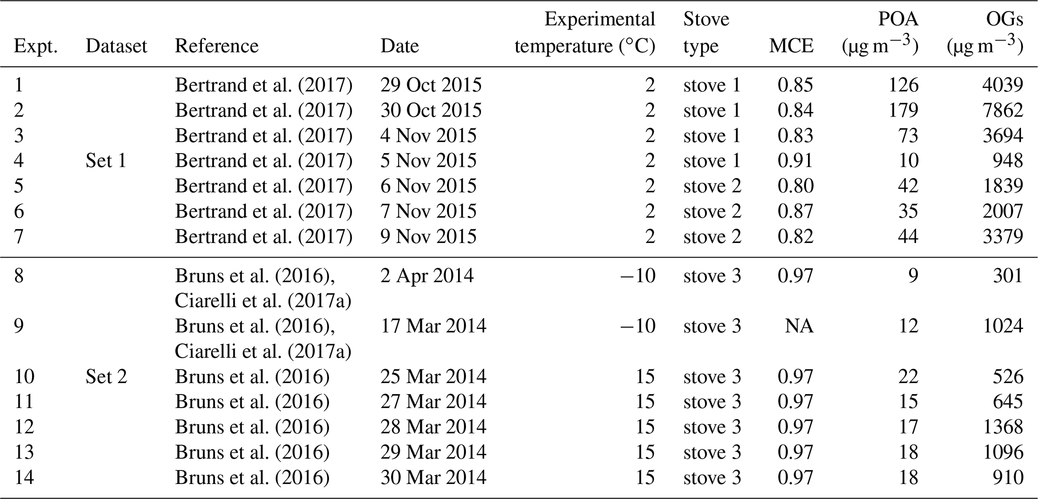
NA: not available.
Ward and Hardy (1991) define the flaming and smoldering conditions according to the modified combustion efficiency, . Specifically, MCE > 0.9 is identified as the flaming condition, while MCE < 0.85 is identified as the smoldering condition. MCE values for the different experiments are reported in Table 1. According to this parameter, Set 1 and Set 2 experiments were dominated by smoldering and flaming, respectively. Practically, we achieved the different burning conditions by varying the amount of air in the stoves, therefore changing the combustion temperature. For Set 1, closing the air window decreased the flame temperature, resulting in a transition from a flaming to a smoldering fire. This could be visibly identified, together with the development of a thick white smoke from the chimney. We note that this conduct is very common in residential stoves, to keep the fire running for longer. Meanwhile, for Set 2, after lighting the fire, we kept a high air input to maintain a flaming fire. At the same time, we monitored the MCE in real time and only injected the emissions into the chamber when the MCE increased above 0.9.
The experiments were performed in a flexible Teflon bag of nominally 7 but typically about 5.5 m3 equipped with UV lamps (40 lights, 90–100 W, Cleo Performance, Philips, wavelength λ<400 nm) enabling photo-oxidation of the emissions (Platt et al., 2013; Bruns et al., 2015). The chamber is located inside a temperature-controlled housing. Relative humidity was maintained at 50 % and three different temperatures were investigated. Emissions from the stoves were sampled from the chimney into the chamber through heated (140 ∘C) stainless-steel lines to reduce the loss of semi-volatile compounds. An ejector dilutor was installed (Dekati Ltd, DI-1000) to dilute emissions in the chamber by a factor of 10 before sampling. The sample injection lasted for approximately 30 min for each experiment, and was followed by an injection of 1 µL d9-butanol (98 %, Cambridge Isotope Laboratories), which was used to estimate the OH exposure as described in Sect. 3.1.1 (Barmet et al., 2012). The chamber was then allowed to equilibrate for 30 min to ensure stabilization and homogeneity and to fully characterize the primary emissions before ageing. OH radicals were produced by UV irradiation of nitrous acid (HONO) injected after chamber equilibration, generated as described in Taira and Kanda (1990) by reaction of diluted sulfuric acid (H2SO4) and sodium nitrate (NaNO2) in a gas flask followed by transportation into the chamber with a carrier gas with a flow rate of 1 L min−1. The smog chamber was then irradiated with UV lights for approximately 4 h to simulate atmospheric ageing.
Before and after each experiment, the smog chamber was cleaned with humidified pure air (100 % RH) and O3 (1000 ppm) under irradiation with UV lights for at least 1 h, followed by flushing with pure dry air for at least 10 h. The background particle- and gas-phase concentrations were then measured in the clean chamber.
The total amount and composition of the emissions depend on the oxygen supply, temperature, fuel elemental composition and combustion conditions, which can be broadly classified as flaming or smoldering (Koppmann et al., 2005; Sekimoto et al., 2018). Flaming combustion occurs at high temperature and consists of volatilization of hydrocarbons from the thermal decomposition of biomass leading to rapid oxidation and efficient combustion, producing CO2, water and black carbon (BC). Instead, smoldering combustion is flameless and can be initiated by weak sources of heat and results in less efficient combustion of fuel, leading to gas-phase products (mainly CO, CH4 and volatile organic compounds).
2.2 Instrumentation
We characterized the emissions with a suite of gas- and particle-phase instrumentation. Organic gases (OGs) were measured by a proton-transfer-reaction time-of-flight mass spectrometer (PTR-ToF-MS 8000, Ionicon Analytik). A detailed description of the instrument can be found in Jordan et al. (2009). The PTR-ToF-MS was operated under standard conditions (ion drift pressure of 2.2 mbar and drift intensity of 125 Td) in H3O+ mode, allowing the detection of OGs with a proton affinity higher than that of water. Quantification was performed by using known individual reaction rate constants (Cappellin et al., 2012), otherwise a value of cm3 s−1 was assumed. The effective rate constants applied to both Set 1 and Set 2 can be found in Bruns et al. (2017). Data were analysed using the Tofware software 2.4.2 (PTR module as distributed by Ionicon Analytik GmbH, Innsbruck, Austria) running in Igor Pro 6.3.
Non-refractory primary and aged particle composition was monitored by a high-resolution time-of-flight aerosol mass spectrometer (HR-ToF-AMS, Aerodyne Research Inc.) (DeCarlo et al., 2006). The HR-ToF-AMS is described in detail elsewhere (Bruns et al., 2016; Bertrand et al., 2017) and summarized here. The instrument was operated under standard conditions (temperature of vaporizer 600 ∘C, electronic ionization (EI) at 70 eV, V mode) with a temporal resolution of 10 s. Data analysis was performed in Igor Pro 6.3 (Wave Metrics) using SQuirrel 1.57 and Pika 1.15Z assuming a collection efficiency of 1. The O : C ratio was determined according to Aiken et al. (2008).
The concentration of equivalent black carbon (eBC) was determined from the absorption coefficient measured with a seven-wavelength Aethalometer (Magee Scientific Aethalometer model AE33) with a time resolution of 1 min at a wavelength of 880 nm (Drinovec et al., 2015).
The particle number concentration and size distribution (16 to 914 nm) were provided by a scanning mobility particle sizer (SMPS, consisting of a custom-built differential mobility analyser (DMA) and a condensation particle counter (CPC 3022, TSI)) with a time resolution of 5 min. Supporting gas measurements included a CO2 analyser (LI-COR), a CH4 monitor, a total hydrocarbon (THC) monitor (flame ionization detector, THC monitor Horiba APHA-370), and NO and NO2 (NOx analyser, Thermo Environmental) monitors.
The data analysis entails three steps detailed in this section. The first subsection describes the determination of the amount of oxidized OGs in the chamber. The second subsection details the determination of the amount of SOA formed in the chamber. The last subsection describes the box model used for the parameterization of SOA formation from the OGs.
3.1 Organic gas loss in the chamber
In the chamber, OGs were oxidized to several oxidation products, referred to as oxidized OGs (CG, condensable gases) in the following analysis. According to their volatility, these products may remain in the gas phase or partition to the particle phase, thereby contributing to SOA formation.
We described the change in any OG concentration over time as a combination of its loss and production as follows:
Here, P corresponds to the production of an OG in the chamber, e.g. from the oxidation of other primary OGs. kdil is the dilution rate constant in reciprocal seconds. kOH [OH] [OG] in molecules per cubic centimetre per second represents the consumption rate due to oxidation by OH, where kOH is the reaction rate constant and [OH] is the OH concentration. kother[OG] in molecules per cubic centimetre per second is the loss rate of OG by other processes, where kother is the reaction rate constant in reciprocal seconds. The loss of some OGs could not be explained by their reaction with OH and dilution alone for Set 1, so we added this additional term, which is discussed after the first two processes are constrained. We considered primary OGs that exhibited a clear decay with time to be strictly of primary origin, and hence neglected their production from other OGs (i.e. P=0). This assumption signifies that the yields estimated under our conditions are upper limits. In reality, the detection of aromatic hydrocarbons (e.g. single-ring aromatic hydrocarbons, SAHs, and polycyclic aromatic hydrocarbons, PAHs) by the PTR-ToF-MS may be affected by the interference due to fragmentation during ionization of their oxidation products (Gueneron et al., 2015). On the other hand, directly emitted oxygenated aromatics could themselves be the oxidation products of aromatic hydrocarbons and their production may continue during the experiment. However, the assumption of P=0 does not introduce a significant error for most OGs with significant primary emissions because the observed OG decay was consistent with their OH reaction rate constant for Set 2 as demonstrated by Bruns et al. (2017) for the +15 ∘C conditions. In the following, we describe the processes governing the changes in the OG concentrations in the chamber and the approaches adopted for the determination of the different parameters in Eq. (1).
3.1.1 Reaction with OH radical
The OH exposure, which is the integrated OH concentration over time, was estimated based on the differential reactivity of two OGs. Specifically, we used d9-butanol (fragment at mass-to-charge ratio m∕z 66.126, [C4D9]+) and naphthalene (fragment at m∕z 129.070, [C10H8]H+). These compounds are selected because they can be unambiguously detected (no isomers or interferences, high signal-to-noise ratio), are not produced during the experiment and have OH reaction rate constants that are precisely measured and significantly different from each other. The OH exposure can be expressed as follows:
where (d9-butanol ∕ naphthalene)0 is the ratio between these compounds at t=0 (before lights were turned on), (d9-butanol ∕ naphthalene)t is the ratio measured at time t, and kOH,but and kOH,naph are the OH reaction rate constants of d9-butanol and naphthalene, respectively ( cm3 molec.−1 s−1 and cm3 molec.−1 s−1) (Atkinson and Arey, 2003).
For Set 1, the OH exposure at the end of each experiment ranged between 5 and 8×10⁶ molec. cm−3 h, corresponding to approximately 5–8 h in the atmosphere (given global average and typical wintertime OH concentrations of 1×10⁶ molec. cm−3). For Set 2, higher OH exposures were reached (3 to 7×10⁷ molec. cm−3 h at the end of each experiment, corresponding to 2–3 d in the atmosphere). This is likely because both sets of experiments utilized a similar HONO molar flow (and thus similar OH production rate), but higher OG concentrations were reached in Set 1, which could possibly have resulted in a higher OH sink. We calculated the OH concentration, [OH] in Eq. (1), numerically as d(OH exposure)∕dt.
3.1.2 Smog chamber dilution
For Set 2, dilution was dominated by the constant injection of HONO to the chamber and accounted for as described in Bruns et al. (2016). For Set 1 the dilution rate of primary OGs in the chamber was calculated as follows. The integrated dilution over time, Kdil, was determined as the ratio between the d9-butanol concentration corrected for the reaction of d9-butanol with OH and the d9-butanol concentration at ):
Figure S1 shows calculated values for Kdil as a function of time. Increasingly high dilution at the end of these experiments (Fig. S1), between 20 % and 35 % (i.e. a dilution ratio of 0.8 to 0.65), is a result of constant injection of HONO and excessive sampling at high rates, resulting in inputs from laboratory air (likely through leaks in the Teflon bag or the connections of chamber inlets and outlets). The inputs from the HONO pure carrier gas and of laboratory air are roughly comparable (about 12 % vs. 8 %–23 % at the end of the experiment). Other than dilution, the effect of both inputs on the gas-phase chemical composition is negligible. Dilution rates are non-linear, increasing as the experiment progresses due to continuous dilution within a decreasing chamber volume. The dilution rate constant, kdil, in Eq. (1), is the differential of Kdil over time.
3.1.3 Losses by other processes
To corroborate the estimated OH exposures and dilution rates, we examined the loss of prominent OGs with known reaction rate constants against OH. For Set 2 and as demonstrated by Bruns et al. (2017), the OG decay is consistent with their estimated loss based on their dilution and reaction with OH. By contrast, for Set 1, the decay of some OGs could not be solely explained by their reaction with OH and dilution, suggesting additional reactions with oxidants other than OH as discussed below. The OG total consumption by this process (∫kother[OG]) was estimated as the difference between the total measured decay of the OG of interest and the fraction consumed by both dilution and oxidation by OH radicals. The reaction rate constants for several precursors towards OH (kOH) are not available in the literature. In addition, many fragments may have several isomers, each of which is associated with different rate constants. Effective rate constants for all precursors considered were estimated from their decay in Set 2, where the combination of OH reaction and dilution fully explained the decay of OGs with known OH reaction rate constants.
3.1.4 Precursor classification
A common set of 263 ions was extracted from the PTR-ToF-MS. Among these ions, 86 showed a clear decay with time and were thus identified and selected as potential SOA precursors. Previous work based on Set 2 experiments showed that the PTR-ToF-MS measures the most important SOA precursors, which explained the measured SOA mass within 40 % uncertainty and without systematic bias (Bruns et al., 2016). Therefore, these compounds are expected to capture the dominant fraction of SOA mass, although we cannot rule out losses in the PTR-ToF-MS inlet or small contributions from other precursors such as alkanes. The compound identification was supported by previous publications (McDonald et al., 2000; Fine et al., 2001; Nolte et al., 2001; Schauer et al., 2001; Stockwell et al., 2015), including gas chromatography–mass spectrometry (GC–MS) analysis when available.
The size of our dataset does not allow us to retrieve the volatility distribution for single precursors, which would entail the determination of more than 86 free parameters. This is especially the case as the time series of precursors, decaying with oxidation, are typically strongly correlated, which prevents resolving systematic differences between the yields of the different single precursors. Therefore, lumping is needed to decrease the model degree of freedom. Accordingly, precursors are grouped in six chemical classes: furans, single-ring aromatic hydrocarbons (SAHs), polycyclic aromatic hydrocarbons (PAHs), oxygenated aromatics (OxyAH) and organic compounds containing six and more or fewer than six carbon atoms (OVOCc ≥ 6 and OVOCc < 6, respectively) (Table S1). The selected precursors in each class are the same for each experiment and each dataset. This lumping approach is based on the two main objectives of the study:
-
Compare the SOA yields of specific precursors determined in complex emission experiments with those determined in single-compound systems.
-
Identify the main SOA precursors in flaming and smoldering wood emissions, at different temperatures.
To be able to compare to literature yields, we lumped species that have similar yields in the same chemical class: e.g. at an organic aerosol concentration of 10 µg m−3 the yield of PAHs is ∼ 20 % (objective 1). In addition, we classified the precursors based on the pathway by which they are emitted, which will allow us to determine which compounds dominate SOA formation in flaming and smoldering emissions (objective 2). We differentiated between oxygenated aromatics, mainly emitted through lignin pyrolysis, furans emitted through cellulose pyrolysis, and single-ring aromatics and PAHs generated from incomplete combustion, especially from flaming wood. The remaining SOA precursors are all oxygenated OGs; therefore we separated them according to their carbon number knowing that larger precursors will have higher yields than smaller precursors. Our ability to precisely extract yields specific to a precursor class heavily relies on differences in the oxidation rates or emission patterns of the precursors. Therefore, the classification approach adopted here, where classes are expected to have different contributions during different experiments (Bhattu et al., 2019), facilitates the extraction of yields of the different classes.
3.2 Calculation of the OA mass in the chamber
The total organic aerosol measured by the HR-ToF-AMS was corrected for particle losses in the chamber due to gravitational and diffusional deposition. To assess the total wall losses due to both processes, we assumed that the condensable vapours partition only to the suspended aerosols but not to the wall.
Assuming that black carbon is inert in the chamber, it was possible to use its decay to estimate the particle loss to the walls. The aerosol attenuation measured at 880 nm (at the end of each experiment, ∼ 4 h) with an Aethalometer was used to estimate the particle loss rate to the wall. This attenuation is proportional to the eBC mass concentration and within uncertainties independent of the ageing extent, as demonstrated in Kumar et al. (2018). Using eBC as a tracer, we inherently assumed that eBC and OA were internally mixed and homogeneously distributed over the aerosol size range. The decay of eBC due to both dilution and deposition onto the chamber walls was parametrized as follows:
where kwall is the first-order wall loss rate constant used to correct the measured OA concentration for wall losses, ranging between 4 and s−1, and kdil is the dilution rate constant determined above.
The wall-loss-corrected organic aerosol, OAWLC, was calculated using Eq. (5):
where OA(t) is the measured organic aerosol concentration in microgram per cubic metre. The total OA present in the chamber was estimated as the suspended OA concentration measured by the HR-ToF-AMS plus the estimated OA lost to the wall. This concentration was directly compared to the condensable gas (CG) concentration estimated according to Eq. (A8) presented in Appendix A. As mentioned, our approach did not take into account the losses of precursor vapours or their oxidation products in the gas phase onto the walls. We note that these processes were unlikely to have a substantial effect on the precursors considered, which were largely highly volatile species, even at lower temperature. Based on the calculation of the equilibrium constant of semi-volatile species on the walls by Bertrand et al. (2018b), we estimated that at 293 K the fraction of these compounds absorbed on the walls is < 5 %. Meanwhile, the walls could indeed act as a sink for the semi-volatile oxidation products. This effect was not taken into account in the current study, but we expect that it was minimized under our conditions, by the high OA concentration in the chamber and high production rates (Zhang et al., 2014; Nah et al., 2017).
3.3 Modelling SOA formation
The general aim of the model is the determination of the parameters describing the volatility distributions of the oxidation products from different precursor classes and their temperature dependence. A simplified schematic of the modelling framework is described in Fig. 1. It consists of (1) a box model that describes the partitioning of the condensable gases generated through oxidation, (2) the model input parameters obtained from the smog chamber, (3) the model output parameters and (4) the model optimization based on a genetic algorithm (GA). Each of these parts is described in the following sections.
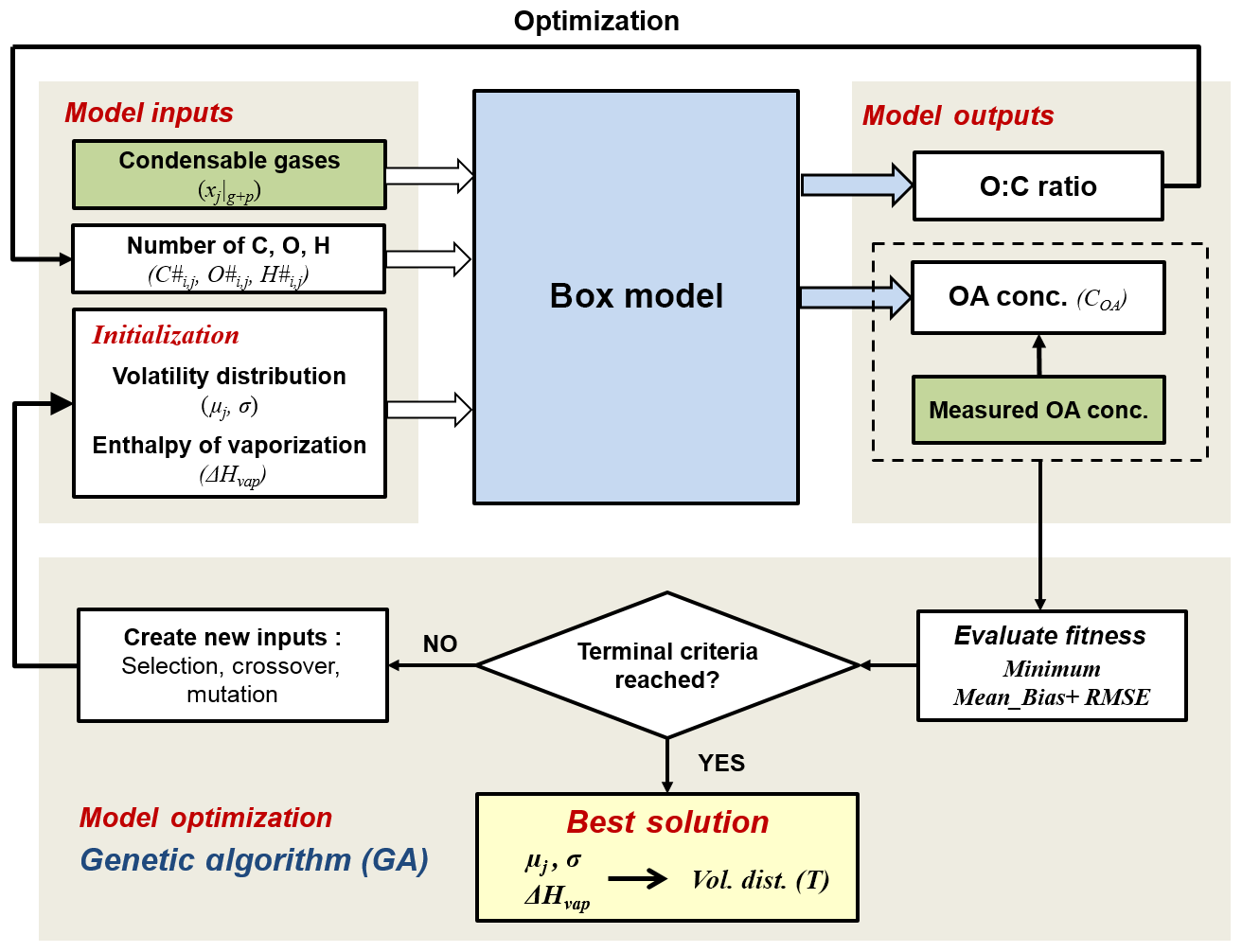
Figure 1Schematic of the modelling framework. The box model simulates the formation of SOA from each precursor class j in volatility bins i. The best solution of the initialized input parameter volatility distribution (described as the mean value of logC* for each precursor class μj and standard deviation σ) and enthalpy of vaporization (ΔHvap) parameters are optimized by a genetic algorithm, using minimum mean bias and root-mean-square error (RMSE) between modelled and measured OA concentration as the fitness function. Green boxes represent measured data from the chamber experiments.
3.3.1 Box model
We assume the partitioning of CG between the gas and the particle phases to obey Raoult's law (Strader et al., 1999), where the aerosol can be described as a pseudo-ideal organic solution, of SOA and POA species. The volatility basis set (VBS, implemented by Koo et al., 2014, in the Comprehensive Air quality Model with eXtensions, CAMx) was used to classify the oxidation products of the different precursors into surrogates with different volatility, distributed into discrete logarithmically spaced bins (Donahue et al., 2006).
We considered the most basic mechanism by which SOA may form. That is, the oxidation products from the different precursor classes described above instantaneously partition into the condensed phase depending on their volatility. No additional reactions in the gas or particle phase were considered (e.g. reaction with oxidants, photolysis or oligomerization). In addition, we neglected the contribution of primary oxidation products of the gas-phase semi-volatile species (co-emitted with POA) compared to the OGs detected by the PTR-ToF-MS, based on the findings of Bruns et al. (2016) and Ciarelli et al. (2017a). Finally, we considered the species in the gas and the particle phases to be permanently at equilibrium, as condensation is expected to be faster than oxidation (timescales for oxidized vapour condensation < 1 min assuming no particle-phase diffusion limitations; Bertrand et al., 2018b). While including additional processes in the model is feasible, this would result in a significantly higher-dimensional parameter space, which cannot be unambiguously inferred from the present data. We consider that without supportive data, e.g. chemically resolved characterization of the particle-phase species, such reactions could not be well constrained or even deduced from structure activity relationships, given the many unknowns in complex emissions. Therefore, such a simplified scheme of SOA formation from complex emissions may be compared in the future with chemically resolved data to help the identification of additional mechanisms that were not considered here.
The derivation of the thermodynamic equations governing SOA formation from precursors, implemented in the box model, is detailed in Appendix A and only a brief description of the model principles is given here. In the following, let i and j be the indices for the different volatility bins and precursor classes, respectively. The model determines the molar distribution of the oxidation products from different precursor classes in the different volatility bins, Υi,j, together with the compounds' enthalpy of evaporation, . The latter describes the temperature dependence of the oxidation products' effective molar saturation concentration, . For this, the model iteratively solves Eqs. (A6) and (A7) at every experimental time step (time resolution of 10 s) for all experiments, to retrieve the surrogate molar concentrations in the particle phase, xi,j|p, and the total surrogates' molar concentration in the condensed organic phase, xOA (see Appendix A).
3.3.2 Model inputs
The model uses as main inputs the molar concentrations of the condensable gases from different precursors (in total n= six precursor classes) in both phases, xj|g + p. The concentration of condensable gases in both the gas and particle phases is derived from the consumption rates of VOCj determined by the PTR-ToF-MS, by numerically integrating Eq. (A8). xj|g + p is related to the concentrations of the different surrogates from a precursor class j in different volatility bins, (Eq. A6), through their yields, Υi,j, according to Eq. (A9). The number of volatility bins, m, is set to six, approximately corresponding to the following mass saturation concentrations: .
In addition to xj|g + p, the model needs as input , the molar concentration of primary organic matter from a volatility bin i in both gas and particle phases (Eq. A7). is inferred from the measured POA concentrations injected in the chamber at the beginning of the experiment and using the volatility distribution function of wood combustion emissions in May et al. (2013). It is assumed constant with ageing. The computation of the fraction of POAi in the condensed phase is similar to that for SOA species in Eq. (A6).
The secondary surrogates' elemental composition (C#i,j, O#i,j and H#i,j) is also used as model input to compute the surrogates' molecular weight, MWi,j, required for COA calculations (see Sect. 3.3.3). A single C#i,j value is calculated per chemical class, based on the average of the respective precursor class, and considering , where ΔC is the average loss in carbon due to fragmentation during the oxidation of precursors from all classes. ΔC is determined by systematically changing its value in multiple model runs and selecting the value that best explains the observed O : C ratios (see Fig. 8b). Likewise, a single H#i,j value is assumed per chemical class, considering that H#j∕C#j equals . Finally, O#i,j is constrained by the C#j and the surrogate volatility () based on the simplification of the SIMPOL model (Pankow and Asher, 2008), provided by Eq. (3) in Donahue et al. (2011). Based on this relationship, O#i,j increases with decreasing C#j and . The O : C ratio of primary emissions is constrained in the model to the measured O : C in the beginning of each experiment, by setting and calculating using the same methodology as for O#i,j. The resulting and and the corresponding primary organic matter molecular weight, MW, as well as C#j, O#i,j, H#j and MWi,j, is reported in Table S4.
3.3.3 Model outputs
The model provides the Υi,j and parameters. To reduce the model's degree of freedom we consider a single ΔHvap for all surrogates from different chemical classes in different volatility bins. Υi,j is considered to follow a kernel normal distribution as a function of log C*, , where μj is the median value of log C* and σ is the standard deviation. This step (1) ensures positive Υi,j parameters, (2) significantly reduces the model's degree of freedom and (3) allows constraint of the total concentration of surrogates from a certain chemical class: .
The set of Υi,j and parameters is determined by minimizing the sum of mean bias (MB) and the root-mean-square error (RMSE) between modelled mass concentrations of the particulate organic phase, COA, calculated using Eq. (6), and concentrations measured by the AMS.
The model fitted to the measured COA was also validated by external AMS measurements of the O : C ratio determined through high-resolution analysis. The modelled O : C ratio was calculated at every experimental time step as follows:
3.3.4 Model optimization
The model is optimized to determine the volatility distributions of the oxidation products from different precursor classes described by μj, σ and their temperature dependence described by ΔHvap to best fit the observed OA concentrations. For the model optimization, we used a genetic algorithm (GA), a metaheuristic procedure inspired by the theory of natural selection in biology, including selection, crossover and mutation processes, to efficiently generate high-quality solutions to optimize problems (Goldberg et al., 2007; Mitchell, 1996). The GA is initiated with a population of randomly selected individual solutions. The performance of each of these solutions is evaluated by a fitness function, and the fitness values are used to select more optimized solutions, referred to as parents. The new generation of solutions (denoted children) is produced by either randomly changing a single parent (as mutation) or combing the vector entries of a pair of parents (as crossover). The evolution process will be repeated until the termination criterion is reached, here maximum iteration time. In this study, a population of 50 different sets of model parameters (μj, σ and ΔHvap) was considered for each GA generation. The sum of mean bias and RMSE between measured and modelled COA of the 14 experiments was used as a fitness function to evaluate the solutions. We assume the termination criterion is reached if no improvement in the fitness occurs after 50 generations, with a maximum of 500 total iterations allowed. The GA calculations were performed using the package “GA” for R (Scrucca et al., 2017). A bootstrap method was then adopted to quantify the uncertainty in the constrained parameters.

Figure 2Comparison of the OG emissions between the two sets of experiments. Panels (a) and (b) display average primary OG mass spectra from Set 1 (representing the smoldering phase) and Set 2 (representing mainly the flaming phase), respectively. Spectra are normalized to the initial total OG concentration in micrograms per cubic metre. Compounds are colour coded by chemical classes. (c) The p value vs. fold change comparing the fingerprints of primary OGs between the two sets of experiments. The fold change was calculated as the ratio of the intensities of each ion normalized to the total signal, between Set 2 and Set 1 averaged across experiments. Data points above p=0.05 have significantly different contributions to the total OGs between the two sets of experiments. Blue coloured data points on the right-hand side designate compounds enriched in the emissions from Set 2 while green coloured data points on the left-hand side designate compounds enriched in the emissions from Set 1. (d) Spearman correlation matrix for the primary OG mass spectra between all experiments highlighting the variability in the composition of the primary emissions. Each experiment is identified by an index (see Table 1) and the experiments from Set 2 were reordered according to similarity with Set 1.
4.1 Comparison of primary emissions across experiments
A larger amount of primary OG was emitted into the chamber in Set 1, with concentrations ranging from 950 to 7860 µg m−3, while in Set 2 the primary OG concentrations ranged from 300 to 1360 µg m−3. In the same way, the measured OA at the beginning of each test (POA) ranged from 10 to 180 µg m−3 and from 9 to 22 µg m−3 for Set 1 and Set 2, respectively (Table 1). The OG composition for Set 1 and Set 2 is summarized in Fig. 2 showing the mean PTR-ToF-MS mass spectra (Fig. 2a, b), the relative contributions of the different compounds for different datasets (Fig. 2c) and the variability in composition among all experiments (Fig. 2d). Set 1 shows higher relative contributions of furans and OVOCc < 6 (Fig. 2a), while the contributions of PAH, SAH and OxyAH are higher in Set 2 (Fig. 2b). The OxyAH compounds, mainly methyl- and methoxyphenols, are produced by lignin pyrolysis (Fine et al., 2001) while furans are formed from cellulose pyrolysis (Mettler et al., 2012). The chemical class referred to as “Others” comprises compounds that do not show a clear decay upon oxidation and are therefore not considered SOA precursors in the following analysis. The category others is dominated by acetic acid, previously reported as a major species in residential wood burning emissions (Bhattu et al., 2019). The majority of the compounds differ among datasets and the most significant difference estimated through the p value (probability associated with a Student's t test) occurs for the OVOCc < 6, which is about a factor of 6 higher than the significance threshold (p=0.05) for Set 1. In order to investigate the similarity between all experiments a Spearman correlation matrix was calculated. Experiments from Set 1 appear to be consistently similar to each other while the experiments from Set 2 are significantly different among each other in terms of composition of the primary emissions. A possible reason for such a discrepancy was the difficulty in injecting flaming emissions without any significant smoldering contribution for Set 2. This hypothesis is supported by the strong similarity between precursor compounds measured in some experiments supposed to represent flaming-phase emissions only but apparently included some smoldering as well (9, 12, 13) and experiments from Set 1 (1–7). Figure S2 reports the relative contributions of primary OGs (before photo-oxidation) for all compound classes for the 14 experiments. Note that these trends are not correlated with the modified combustion efficiency (MCE), reported in Table 1, defined as , which was constant at 0.97 g g−1, for Set 2, but ranged from 0.8 g g−1 to 0.91 g g−1 for Set 1.
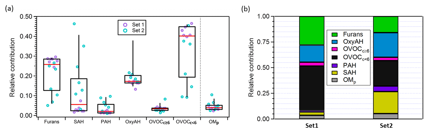
Figure 3(a) Box plot for the relative contributions to the total primary emissions of the different precursor classes and of OMp averaged between experiments. OMp is the total semi-volatile and low-volatility organic matter calculated by means of the VBS model assuming the volatility distribution from May et al. (2013) and using as input the measured organic aerosol (OA) mass. The top and bottom whiskers represent the 90th and 10th percentiles, respectively, while the top, middle and bottom lines of the boxes show the 75th, 50th and 25th percentiles, respectively. The circles represent each single experiment from the two datasets investigated. (b) Average contributions of different precursor families and OMp for Set 1 and Set 2.
Figure 3 shows the contribution of each class of precursor compounds and of the primary semi-volatile organic matter (OMP) to the total primary emissions. OMP is the total organic matter in the semi-volatile and low-volatility range in the particle and the gas phases (saturation concentration < 1000 µg m−3 at 298 K) (see Sect. 3.3.2). Overall, the highest average relative contributions are related to OVOCc < 6 followed by furans and OxyAH, but we also note an average large contribution by SAH for Set 2. The two sets of experiments investigated clearly show different primary composition of emissions in terms of dominant contributions; in Set 1 OVOCc < 6 and OxyAH dominate by far the total primary emissions while in Set 2 the main species influencing the total primary emissions are OxyAH, OVOCc < 6 and SAH with roughly similar contributions (see Fig. 3b). Moreover, the calculated averaged OMp ∕ OGs ratios are around 0.05 and 0.03 for Set 2 and Set 1, respectively.
OGs undergo oxidation during atmospheric ageing to form a complex mixture of products, some of which remain in the gas phase while others have sufficiently low volatility to partition to the particle phase. The consumption of the different OG classes over time is shown in Fig. 4a, b for Set 1 and Set 2, respectively. The general trends manifest that PAH and OxyAH are the most reactive classes, exhibiting an average consumption of up to 80 % at the end of the experiments (after ∼ 4 h of ageing) while for both datasets SAH appears to be the least reactive class (with an average consumption between 10 % and 20 % at the end of the experiments). Relevant compounds in the latter class are benzene (C6H6), toluene (C7H8) and xylene (C8H10); their slow reactivity is consistent with literature reaction rate constants toward OH, from the NIST database (NIST chemistry WebBook, Linstrom and Mallard, 2018), of , and (cm3 molec.−1 s−1), respectively.
The two datasets differ for the OH dose; we observe in Set 2 (Expt. 8–14) an overall higher consumption of all precursor classes due to the higher OH dose (representing a longer ageing time in an ambient atmosphere). PAH shows the highest reactivity followed by OxyAH while for Set 1 (Expt. 1–7) the fastest class of compounds to react is the OxyAH followed by PAH and OVOCc < 6. Moreover, despite the lower OH exposure reached for Set 1, the consumption of OxyAH and furans is substantially higher at comparable exposure levels.
Table 2Reported average reaction rate constants (10−11 cm3 molec.−1 s−1) towards OH per family at the beginning of each experiment, including average reactivity (AVG) and standard deviation (SD).

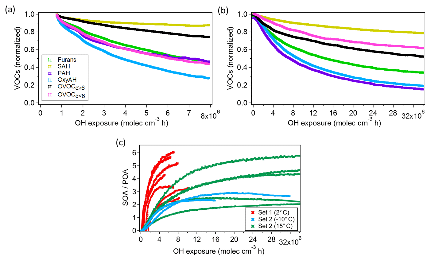
Figure 4Average consumption of SOA precursor classes against average OH exposure for Set 1 (a) and Set 2 (b). The observed decay of SOA precursor families (OGs) as described in Eq. (1) is due to both oxidation processes and dilution in the chamber. (c) SOA-to-POA ratio for each experiment against average OH exposure coloured according to experimental temperatures (2, −10, 15 ∘C).
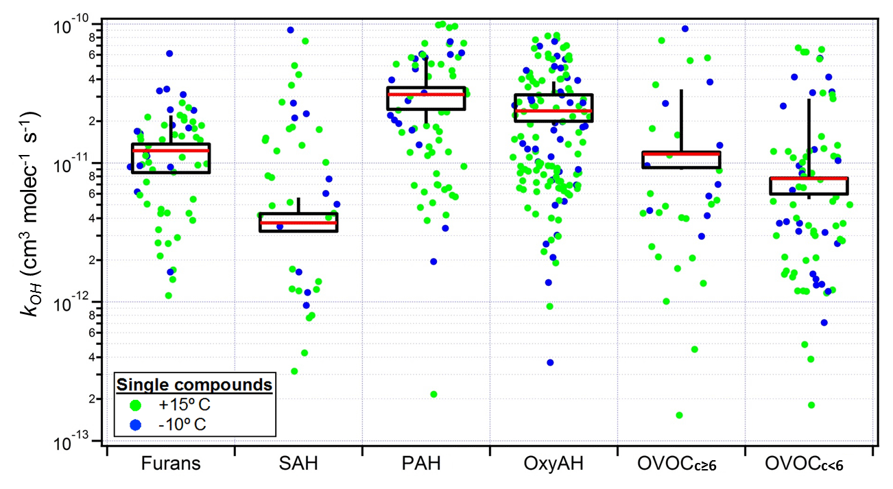
Figure 5Box plot of mass-weighted average OH reaction rate constants (kOH) determined for each precursor class from Bruns et al. (2016) for Set 2 only (see Table S3). The individual kOH values for all compounds are also shown for all experiments, colour coded according to the experimental temperatures. The top and bottom whiskers represent the 90th and 10th percentiles, while the top, middle and bottom lines of the boxes show the 75th, 50th and 25th percentiles, respectively.
In the same way, we also observe a higher SOA production for Set 1 compared to Set 2 at comparable OH exposure. The SOA-to-POA ratio ranges between 2 and 6, similar to ratios observed in previous studies (Heringa et al., 2011; Bruns et al., 2015; Grieshop et al., 2009; Tiitta et al., 2016).
Overall the same chemical classes appear to behave differently across the different sets of experiments. Such an inconsistency in behaviour is due to either differences in the chemical composition within the same class or due to additional reactivity occurring in Set 1.
To investigate the chemical differences within the same class of compounds across different experiments, Table 2 reports the average reaction rate constants against OH of the different chemical classes calculated at the beginning of each experiment following Eq. (8).
Here, c represents the single compound, j the family and k the experiment. kOH is the reaction rate constant toward OH and OG refers to the primary OGs.
OH reaction rate constants () for each compound were calculated from Set 2 only (Fig. 5), whereas the decay of the precursors contributing most to SOA formation during ageing was compared with the expected decay based on literature. The good agreement indicates that for these experiments the consumption of the precursors was dominated by OH (Bruns et al. 2017). The average OH reaction rate constants () are reported in Table S3. They are determined for each precursor class and calculated with a first-order exponential fitting on the precursors' decay curves previously corrected for dilution.

Figure 6Fraction of consumed precursor compounds for Set 1 by OH oxidation (a), dilution (b) and other reactivity (c) at the end of the experiments. Each point corresponds to a single compound averaged among experiments and normalized to the initial concentration. The colour legend represents the statistically significant deviation from zero reactivity with the investigated reactant (p value).
The average reaction rate constants per family ( are similar among the same families for different experiments, suggesting that the variable behaviour of the chemical classes across different experiments was due to differences in the reactive environment rather than a different chemical composition within a given class.
As introduced in Sect. 3.1.3, the total measured decay of OGs in Set 1 could not be fully explained by dilution and reactivity against OH, suggesting the presence of an additional loss process. To assess the remaining oxidation processes, kOH values were used to estimate the missing loss process for Set 1 according to Eq. (1). In this way the consumed fraction due to OH chemistry, dilution in the chamber and the additional reactivity was calculated for each OG compound family and is shown in Fig. 6. The additional reactivity appears to contribute to the total precursor consumption for most of the classes, with particular relevance for the OxyAH and PAH classes. This is in contrast with the calculated loss for Set 2 (Fig. S3) where the dominant consumption is due to OH.
One possible hypothesis is that the remaining loss process might be due to reaction with the nitrate radical (NO3), which absorbs in the visible region (∼ 500–650 nm) and thus is not efficiently photolysed by the black lights used here (Reed et al., 2016). Figure S4 shows that for Set 1 the NO3 reaction rate constants () for compounds found in the NIST database (Linstrom and Mallard, 2018) (see Table S1) are well correlated with the amount reacted, making nitrate chemistry a likely loss process (Schwantes et al., 2017). We note that while the OH production rate in the chamber is similar for the two sets of experiments, given the same injection rate of HONO, the OH total reactivity is significantly higher for Set 1 because of the injection of ∼ 5 times higher OG concentrations. As a result, the OH concentration is around 1.5×10⁶ vs. 10×106 molec. cm−3 for Set 1 and Set 2, respectively, increasing the availability of OGs for consumption by other processes during Set 1.
4.2 Model evaluation
As previously mentioned, the reaction of the OGs produces oxidation products (CG, condensable gases), which can consequently partition between the gas and particle phases. Their concentration, estimated by accounting for the production minus the loss in the chamber, as described in Eq. (1), was used as input for the box model with the volatility basis set (VBS) scheme. Figure S5 shows the volatility distributions of different precursor classes for Set 1 and Set 2 to assess the influence of different processes occurring in different experiments.
We note that for Set 1 the lower-volatility bins exhibit higher contributions compared to Set 2 but still within 2 standard deviations, such that it is difficult to distinguish statistically different yields for most of the cases. Hence, the total volatility distribution was used to calculate the mass yield instead of a specific one for each dataset (Fig. 9). Mass yields calculated for the specific datasets Set 1 and Set 2 are reported in Fig. S6.
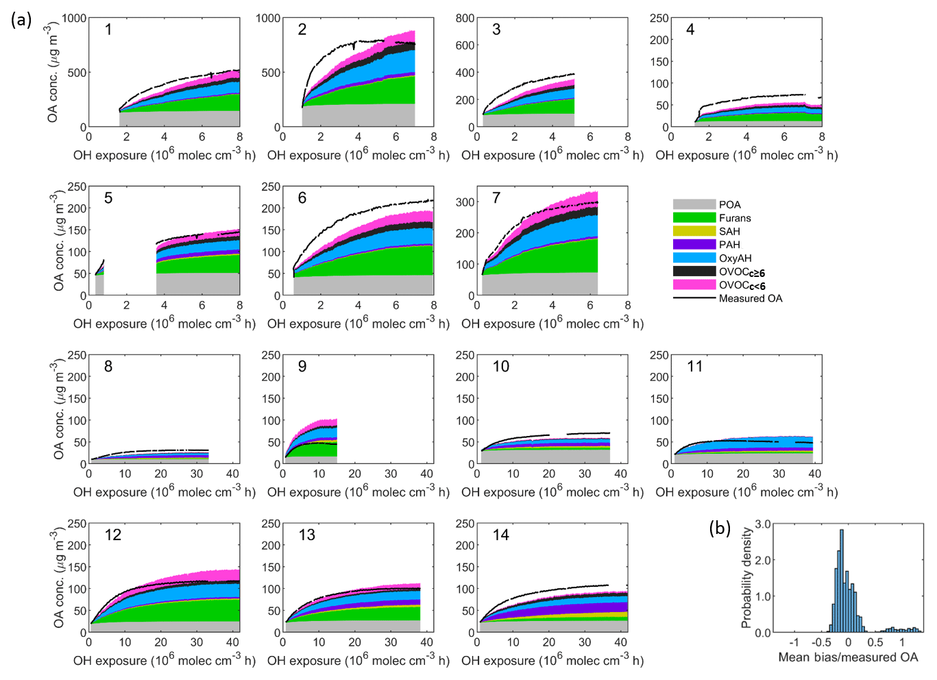
Figure 7(a) Comparison between the sum of simulated organic aerosol (OA) concentrations from different precursor families and the measured OA concentration as a function of the OH exposure for each smog chamber experiment. Set 1 (Expt. 1–7, 2 ∘C) and Set 2 (Expt. 8–9, −10 ∘C and Expt. 10–14, 15 ∘C). (b) Probability distribution of mean bias weighted by the average measured OA concentration. The resulting mean bias is −7.2 µg m−3 (∼ 15 %) and the root-mean-square error (RMSE) is 37.4 µg m−3. The model tends to underestimate the measured OA for Set 1 with a mean bias of 7 % while it tends to overestimate the measured OA for Set 2 with a mean bias of 8 %.
Figure 7 shows the modelled and measured OA mass for all 14 experiments, where Set 1 accounts for both OH and NO3 chemistry while Set 2 includes OH chemistry only. The modelled OA is divided into POA and six SOA classes attributed to the respective precursor classes. Overall, the model performance is satisfactory, although in general the final OA concentration is slightly overpredicted while the initial production rate is underpredicted. Most of the SOA is attributed to furans (30.8 %), OxyAH (19 %) and OVOCc < 6 (12.5 %) for Set 1 while for Set 2 there is a generally lower contribution from OVOCc ≥ 6 (7.8 %) and a higher contribution from PAH (12 %), especially for experiments 08, 13 and 14. The mean bias between measured and modelled OA averaged over all experiments is −7.2 µg m−3, which corresponds to ∼ 15 % on average.
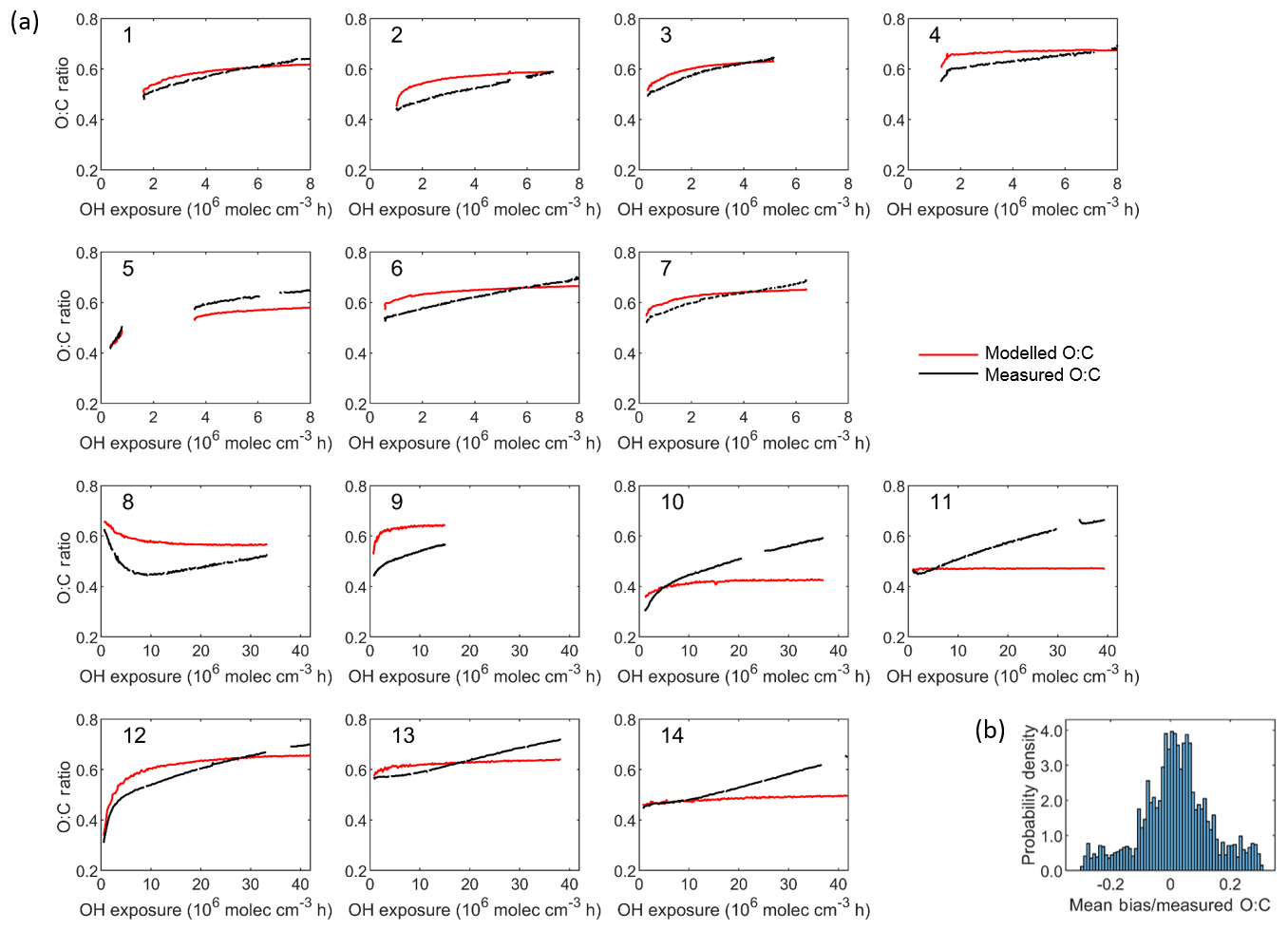
Figure 8(a) Comparison between modelled and measured O : C ratio as a function of the OH exposure for each experiment. Set 1 (Expt. 1–7, 2 ∘C) and Set 2 (Expt. 8–9, −10 ∘C and Expt. 10–14, 15 ∘C). (b) Probability distribution of the relative bias (normalized by the averaged measured O : C ratios). The resulting mean relative bias is 0.006 and the root-mean-square error (RMSE) is 0.06.
4.3 Investigation of OA chemical and physical properties
Comparisons between measured and modelled O : C ratios are reported in Fig. 8. The oxidation products' elemental compositions from which the modelled O : C ratio is calculated are presented in Table S4. The oxidation products' carbon numbers, which best explained the observed O : C ratio, correspond to a set ΔC of 0.6 (Fig. S7). There is a general increase in the O : C ratio with time. Model and observations match in terms of average O : C ratio for each experiment but the temporal evolution of the ratio is not well predicted, suggesting that there are additional processes that are not taken into account in the model. As the model was initiated using the measured POA O : C ratio at OH exposure equal to zero, an agreement between model and measurements can be observed at this time of the experiment. We do not find any systematic correlation of the bias with chamber conditions except for lower concentrations where experiments exhibit higher O : C ratios at the end. Overall for experiments conducted at lower temperature (−10 ∘C) the model tends to overestimate the O : C while for higher-temperature experiments (15 ∘C) the model clearly under-predicts the ratio upon ageing, especially at the end of the experiments, indicating the presence of compounds with a higher number of oxygen molecules (lower number of carbon molecules) than predicted.
Figure 9 shows mass yield curves for each class of compounds, in comparison with mass yields of several single compounds from literature (Table S2). The single compounds were selected according to their presence in the current study and compared to the respective chemical family. The reported published yields were discriminated according to experimental NOx regimes, as low-NOx conditions generally lead to higher OA yields. Our study is more likely representative of a high-NOx regime and thus assesses the SOA forming potential for this atmospherically relevant condition. For the model and measurement conditions (COA∼20–600 µg m−3) the following median mass yields ranges were found: 7 %–20 % for furans, 10 %–25 % for SAH, 14 %–32 % for PAH, 9 %–24 % for OxyAH, 23 %–46 % for OVOCc ≥ 6 and 6 %–18 % for OVOCc < 6. Mass yields were also calculated for the two separate datasets and reported in Fig. S6 in order to assess differences driven by specific combustion regimes. Considering ambient-relevant conditions of COA∼50 µg m−3, we note a generally good agreement between the two datasets except for OxyAH, which exhibit higher median yields (representing smoldering phase) of ∼ 25 % in Set 1 and only ∼ 10 % in Set 2 (representing flaming phase). Set 2 on the other hand exhibited higher median yields for the OVOCc ≥ 6 family (∼ 20 % compared to ∼ 16 % for Set 1).
The effect of temperature and OH exposure on OA concentrations and yields is shown in Fig. 10 for different primary OM loads (total primary gaseous and particulate OMp + OGs) of 6, 60 and 600 µg m−3. The range of temperatures investigated varies between 255 and 315 K. We find a general increase in total OA concentration with increasing OH exposure, decreasing experimental temperature and higher initial loads, as expected. The average increase in OA concentration is 0.001, 0.03 and 0.6 µg m−3 K−1 for 6, 60 and 600 µg m−3, respectively. Concerning SOA yields the temperature effect is also a function of OH exposure and aerosol load; SOA yields increase by 0.0001, 0.0006 and 0.002 g g−1 K−1 on average for 6, 60 and 600 µg m−3, respectively, with a higher effect predicted at lower temperature. We note overall an average yield increase by a factor of 3–4 for a 10-fold increase in the primary OM loads at the highest OH exposure considered (8×10⁷ molec. cm−3 h). Set 2 exhibits higher yields because of lower contributions from the OVOCc < 6 family, which does not produce significant amounts of SOA.
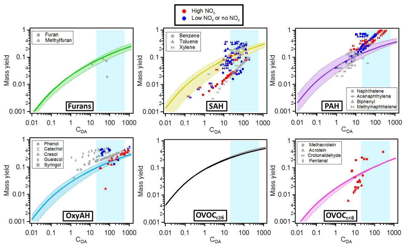
Figure 9Mass yields for each class of compounds. The solid lines represent the median values while the lower and upper limits are the 25th and 75th percentiles, respectively. The different markers in each plot are yields published in the literature for different single compounds (see Table S2). The colour code denotes different NOx regimes (red denoting high NOx, blue low or no NOx and grey not specified NOx regimes). The shaded background represents the range of our experiments (20–600 µg m−3); outside this shaded area yields are extrapolated from the model.

Figure 10Modelled OA concentrations (a) and yields (b) under different temperature, OH exposure and initial OA concentrations (6, 60 and 600 µg m−3). Upper and lower panels are based on Set 1 and Set 2, respectively. Temperature is provided in kelvin (K) to avoid confusion with the experimental data in degrees Celsius (∘C).
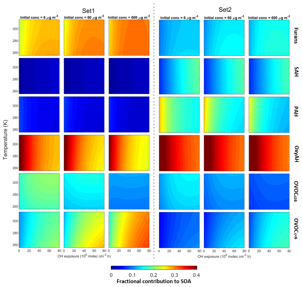
Figure 11Fractional contributions of the six precursor classes to SOA formation under different temperature, OH exposure and initial OA concentrations. Left and right panels are based on Set 1 and Set 2, respectively. Temperature is provided in kelvin (K) to avoid confusion with the experimental data in degrees Celsius (∘C).
SOA yields increase with increasing COA due to additional partitioning but also due to changes in the chemical composition and volatility of SOA species since they age differently with different experimental temperature and concentrations. Compounds with different oxygen-to-carbon ratios lead to different functionality, polarity and vapour pressure upon ageing. Moreover, different temperatures result in different evaporation enthalpies which consequently influence the compounds' volatility and lifetime. The modelled SOA ΔHvap for each family of precursors is 17.5 kJ mol−1 after GA calculation. This value is within the ranges of values reported in literature, where values between 11 and 44 kJ mol−1 were reported for biogenic and anthropogenic SOA precursors depending upon the reactant hydrocarbon mixture and NOx concentration. For SOA formed from both α-pinene and toluene, a negative correlation between ΔHvap and NOx concentration was observed (Offenberg et al., 2006).
The modelled fractional contributions of the six different precursor classes to SOA are shown in Fig. 11 for Set 1 and Set 2. The most dominant contribution is from the OxyAH family apart from Set 1 at high OH exposure where the contributions from precursors with higher volatility (furans and OVOCc < 6) are more strongly temperature-dependent. In detail, the OVOCc < 6 family exhibits a higher contribution with higher initial load and higher OH exposure. The SAH and PAH families have relevant contributions for Set 2 because these compounds are strongly emitted during the flaming phase. Since the SAH family consists of compounds that are less reactive than other families, they become relevant just at high OH exposure, while the compounds in the PAH family react faster and show a decreasing contribution with increasing OH exposure.
We performed box model simulations, based on the volatility basis set (VBS) approach, of residential wood combustion smog chamber experiments conducted at different temperatures, different combustion conditions and using different residential stoves. Primary emissions of SOA precursor compounds (organic gases, OGs) and organic aerosol (OA) as well as their evolution during ageing in the smog chamber were simultaneously monitored by a PTR-ToF-MS and an HR-ToF-AMS, respectively. This enabled the identification of the nature of SOA precursors lumped into different classes according to their chemical composition.
The knowledge about the nature of SOA precursors was used to better constrain model parameters, in the oxidation products' production rates and elemental composition. Using the measured OA mass, we were able to determine the volatility distributions and ΔHvap for the products formed from the oxidation of the dominant precursor compound classes. We estimated the contributions of different compound classes to SOA and evaluate how the variability in the emission composition under a wide range of conditions would influence the SOA yield predictions. Investigation of different experimental temperatures allowed the evaluation of the model evaporation enthalpies, which have a decisive influence on the volatility of the emissions and hence their atmospheric lifetimes. Upon ageing, compounds with lower atomic O : C ratios are converted through the oxidation pathway to products with higher functionality, higher polarity and lower saturation vapour pressure. As a result, a part of these products (re-)condenses to the particle phase with partial pressures determined by their volatility, ambient temperature and concentration of the particulate organic mixture. While the degree of oxygenation increases during ageing, organic species may also fragment into more volatile compounds, being eventually converted into CO2. Understanding the balance between oxygenation and fragmentation, their effect on volatility of emissions and timescale of these processes is essential to predict the evolution of the OA concentration.
Overall we developed a framework useful to constrain complex emissions and suitable for sophisticated mass spectrometry analysis with the novelty and ability of identifying the contributions of different classes of OG precursors to SOA formation. The main focus of the study included the investigation of smoldering vs. flaming emissions, resulting in predominant contributions of different classes of compounds according to the combustion phase investigated. Smoldering-phase emissions were dominated by the OVOCc < 6 compound family while the flaming phase exhibited higher contributions by the SAH and PAH families. For both phases, SOA formation is found to be dominated by OxyAH (e.g. phenols and cresols), emitted from lignin pyrolysis. These species were therefore predicted to be important markers to be monitored in air pollution studies in order to estimate the SOA forming potential from real emissions.
The data of the figures are available at https://doi.org/10.5281/zenodo.3260150 (Stefenelli and el Haddad, 2019).
In this appendix, we present the derivation of the thermodynamic equations used in the model. We considered the species in the gas and the particle phases to be permanently at equilibrium, as condensation is expected to be faster than oxidation (timescales for oxidized vapour condensation < 1 min assuming no particle-phase diffusion limitations; Bertrand et al., 2018b). Accordingly, the relation between the aerosol and gas-phase activities satisfies the following expression:
Here, xi,j|g denotes the gas-phase molar concentration of a surrogate in a volatility bin i formed from a precursor class j. The product represents the activity of the same surrogate in the particle phase, where γi,j and χi,j are the activity coefficient and the fraction of the surrogate in the particle phase, respectively. is the equilibrium molar saturation concentration of the pure surrogate, related to its equilibrium vapour pressure, , according to Eq. (A2).
Here, R and T are the ideal gas constant and the temperature, respectively. The effective molar saturation concentration (), which takes into account the influence of nonideal mixing on the compounds' activity, can be defined as the product of γi,j and :
Similar to , can be written as a function of temperature, according to the Clausius–Clapeyron relationship based on Eq. (A4).
Here, T and Tref are the experimental and reference (Tref=298 K) temperatures, respectively. is the effective enthalpy of evaporation. It includes the effects of temperature on (1) the pure compound saturation vapour pressure (), (2) the compounds' mixing properties in the condensed phase, i.e. γi,j, and (3) the radical chemistry reaction rate constants and branching ratios in the gas phase (Stolzenburg et al., 2018).
is related to the Donahue effective mass saturation concentration (Donahue et al., 2012), , which is the inverse of the Pankow equilibrium constant (Pankow, 1987), through the compounds' molecular weight, MWi,j, as indicated in Eq. (A5).
To constrain the model to the measurements, it is of convenience to rearrange Eqs. (A1) and (A3) as a function of the surrogate total concentration, , and the total molar concentration of species in the particle phase (xOA), which yields the following expression:
The parameters in Eq. (A6) were obtained as follows.
-
The modelled molar concentration of the particulate organic phase was expressed as the sum of the concentration of all surrogates in the particle phase Eq. (A7).
Here, m and n are the total number of volatility bins and precursor chemical classes, respectively. is the particle-phase molar concentration of primary organic matter in volatility bin i. The is calculated based on in both phases, following a similar computation as for SOA (Eq. A6). was inferred from the measured POA concentrations injected into the chamber at the beginning of the experiment and using the volatility distribution function of wood combustion emissions in May et al. (2013).
-
was derived from the precursor oxidation rates measured by the PTR-ToF-MS. The change in the total concentration of oxidation products from a precursor class j in both gas and particle phases, xj|g + p, was expressed as follows:
Here, [OGj] is the molar concentration of total OG precursors in class j. For the definition of the other parameters, the reader is referred to Eq. (1). xj|g + p is calculated by numerically integrating Eq. (A8). xj|g + p is related to the concentration of the different surrogates from a precursor class j in different volatility bins, (Eq. A6), through their yields, Υi,j:
These yields, which represent the surrogate volatility distributions, were determined by the model.
The supplement related to this article is available online at: https://doi.org/10.5194/acp-19-11461-2019-supplement.
GS is the main author. The scientific idea was conceptualized by IEH, JGS, NM and ASHP. The experimental work was performed by GS, AB, EB and SP. The analyses were carried out by GS, IEH, AB and EB. The model has been developed by JJ, IEH and SA. The supervision was performed by JGS, IEH, ASHP and UB. All the authors contributed to writing the paper.
The authors declare that they have no conflict of interest.
We appreciate the availability of the VBS framework in CAMx and support of RAMBOLL.
This research was supported by the Swiss National Science Foundation (project WOOSHI (200021L_140590)) and SNSF Starting Grant IPR-SHOP (BSSGI0_155846), the European Community's Seventh Framework Programme (FP7/2007–2013) under grant agreement no. 290605 (PSI-FELLOW), the European Union's Horizon 2020 Research and Innovation programme through the EUROCHAMP-2020 Infrastructure Activity under grant agreement no. 730997, the Competence Centers Environment and Sustainability (CCES) and Energy and Mobility (CCEM) (project OPTIWARES), and the French Environment and Energy Management Agency (ADEME) under the grant 1562C0019 (VULCAIN project) and the Provence-Alpes-Côte d'Azur (PACA) region.
This paper was edited by Manvendra K. Dubey and reviewed by Marwa Majdi and one anonymous referee.
Aiken, A. C., DeCarlo, P. F., Kroll, J. H., Worsnop, D. R., Huffman, J. A., Docherty, K. S., Ulbrich, I. M., Mohr, C., Kimmel, J. R., Sueper, D., Sun, Y., Zhang, Q., Trimborn, A., Northway, M., Ziemann, P. J., Canagaratna, M. R., Onasch, T. B., Alfarra, M. R., Prevot, A. S. H., Dommen, J., Duplissy, J., Metzger, A., Baltensperger, U., and Jimenez, J. L.: O∕C and OM∕OC ratios of primary, secondary, and ambient organic aerosols with high-resolution time-of-flight aerosol mass spectrometry, Anviron. Sci. Technol., 42, 4478–4485, https://doi.org/10.1021/es703009q, 2008.
Atkinson, R. and Arey, J.: Atmospheric degradation of volatile organic compounds, Chem. Rev., 103, 4605–4638, https://doi.org/10.1021/cr0206420, 2003.
Barmet, P., Dommen, J., DeCarlo, P. F., Tritscher, T., Praplan, A. P., Platt, S. M., Prévôt, A. S. H., Donahue, N. M., and Baltensperger, U.: OH clock determination by proton transfer reaction mass spectrometry at an environmental chamber, Atmos. Meas. Tech., 5, 647–656, https://doi.org/10.5194/amt-5-647-2012, 2012.
Bertrand, A., Stefenelli, G., Bruns, E. A., Pieber, S. M., Temime-Roussel, B., Slowik, J. G., Prévôt, A. S. H., Wortham, H., El Haddad, I., and Marchand, N.: Primary emissions and secondary aerosol production potential from woodstoves for residential heating: Influence of the stove technology and combustion efficiency, Atmos. Environ., 169, 65–79, https://doi.org/10.1016/j.atmosenv.2017.09.005, 2017.
Bertrand, A., Stefenelli, G., Jen, C. N., Pieber, S. M., Bruns, E. A., Ni, H., Temime-Roussel, B., Slowik, J. G., Goldstein, A. H., El Haddad, I., Baltensperger, U., Prévôt, A. S. H., Wortham, H., and Marchand, N.: Evolution of the chemical fingerprint of biomass burning organic aerosol during aging, Atmos. Chem. Phys., 18, 7607–7624, https://doi.org/10.5194/acp-18-7607-2018, 2018a.
Bertrand, A., Stefenelli, G., Pieber, S. M., Bruns, E. A., Temime-Roussel, B., Slowik, J. G., Wortham, H., Prévôt, A. S. H., El Haddad, I., and Marchand, N.: Influence of the vapor wall loss on the degradation rate constants in chamber experiments of levoglucosan and other biomass burning markers, Atmos. Chem. Phys., 18, 10915–10930, https://doi.org/10.5194/acp-18-10915-2018, 2018b.
Bhattu, D., Zotter, P., Zhou, J., Stefenelli, G., Klein, F., Bertrand, A., Temime-Roussel, B., Marchand, N., Slowik, J. G., Baltensperger, U., Prévôt, A. S. H., Nussbaumer, T., El Haddad, I., and Dommen, J.: Effect of stove technology and combustion conditions on gas and particulate emissions from residential biomass combustion, Environ. Sci. Technol., 53, 2209–2219, https://doi.org/10.1021/acs.est.8b05020, 2019.
Bian, Q., Jathar, S. H., Kodros, J. K., Barsanti, K. C., Hatch, L. E., May, A. A., Kreidenweis, S. M., and Pierce, J. R.: Secondary organic aerosol formation in biomass-burning plumes: theoretical analysis of lab studies and ambient plumes, Atmos. Chem. Phys., 17, 5459–5475, https://doi.org/10.5194/acp-17-5459-2017, 2017.
Bozzetti, C., Sosedova, Y., Xiao, M., Daellenbach, K. R., Ulevicius, V., Dudoitis, V., Mordas, G., Byčenkienė, S., Plauškaitė, K., Vlachou, A., Golly, B., Chazeau, B., Besombes, J.-L., Baltensperger, U., Jaffrezo, J.-L., Slowik, J. G., El Haddad, I., and Prévôt, A. S. H.: Argon offline-AMS source apportionment of organic aerosol over yearly cycles for an urban, rural, and marine site in northern Europe, Atmos. Chem. Phys., 17, 117–141, https://doi.org/10.5194/acp-17-117-2017, 2017.
Bruns, E. A., Krapf, M., Orasche, J., Huang, Y., Zimmermann, R., Drinovec, L., Močnik, G., El-Haddad, I., Slowik, J. G., Dommen, J., Baltensperger, U., and Prévôt, A. S. H.: Characterization of primary and secondary wood combustion products generated under different burner loads, Atmos. Chem. Phys., 15, 2825–2841, https://doi.org/10.5194/acp-15-2825-2015, 2015.
Bruns, E. A., El Haddad, I., Slowik, J. G., Kilic, D., Klein, F., Baltensperger, U., and Prévôt, A. S. H.: Identification of significant precursor gases of secondary organic aerosols from residential wood combustion, Sci. Rep.-UK, 6, 27881, https://doi.org/10.1038/srep27881, 2016.
Bruns, E. A., Slowik, J. G., El Haddad, I., Kilic, D., Klein, F., Dommen, J., Temime-Roussel, B., Marchand, N., Baltensperger, U., and Prévôt, A. S. H.: Characterization of gas-phase organics using proton transfer reaction time-of-flight mass spectrometry: fresh and aged residential wood combustion emissions, Atmos. Chem. Phys., 17, 705–720, https://doi.org/10.5194/acp-17-705-2017, 2017.
Cappellin, L., Karl, T., Probst, M., Ismailova, O., Winkler, P. M., Soukoulis, C., Aprea, E., Märk, T. D., Gasperi, F., and Biasioli, F.: On quantitative determination of volatile organic compound concentrations using proton transfer reaction time-of-flight mass spectrometry, Environ. Sci. Technol., 46, 2283–2290, https://doi.org/10.1021/es203985t, 2012.
Chen, J., Li, C., Ristovski, Z., Milic, A., Gu, Y., Islam, M. S., Wang, S., Hao, J., Zhang, H., He, C., Guo, H., Fu, H., Miljevic, B., Morawska, L., Thai, P., Lam, Y. F., Pereira, G., Ding, A., Huang, X., and Dumka, U. C.: A review of biomass burning: Emissions and impacts on air quality, health and climate in China, Sci. Total Environ., 579, 1000–1034, https://doi.org/10.1016/j.scitotenv.2016.11.025, 2017.
Ciarelli, G., El Haddad, I., Bruns, E., Aksoyoglu, S., Möhler, O., Baltensperger, U., and Prévôt, A. S. H.: Constraining a hybrid volatility basis-set model for aging of wood-burning emissions using smog chamber experiments: a box-model study based on the VBS scheme of the CAMx model (v5.40), Geosci. Model Dev., 10, 2303–2320, https://doi.org/10.5194/gmd-10-2303-2017, 2017a.
Ciarelli, G., Aksoyoglu, S., El Haddad, I., Bruns, E. A., Crippa, M., Poulain, L., Äijälä, M., Carbone, S., Freney, E., O'Dowd, C., Baltensperger, U., and Prévôt, A. S. H.: Modelling winter organic aerosol at the European scale with CAMx: evaluation and source apportionment with a VBS parameterization based on novel wood burning smog chamber experiments, Atmos. Chem. Phys., 17, 7653–7669, https://doi.org/10.5194/acp-17-7653-2017, 2017b.
Crippa, M., DeCarlo, P. F., Slowik, J. G., Mohr, C., Heringa, M. F., Chirico, R., Poulain, L., Freutel, F., Sciare, J., Cozic, J., Di Marco, C. F., Elsasser, M., Nicolas, J. B., Marchand, N., Abidi, E., Wiedensohler, A., Drewnick, F., Schneider, J., Borrmann, S., Nemitz, E., Zimmermann, R., Jaffrezo, J.-L., Prévôt, A. S. H., and Baltensperger, U.: Wintertime aerosol chemical composition and source apportionment of the organic fraction in the metropolitan area of Paris, Atmos. Chem. Phys., 13, 961–981, https://doi.org/10.5194/acp-13-961-2013, 2013.
DeCarlo, P. F., Kimmel, J. R., Trimborn, A., Northway, M. J., Jayne, J. T., Aiken, A. C., Gonin, M., Fuhrer, K., Horvath, T., Docherty, K. S., Worsnop, D. R., and Jimenez, J. L.: Field-deployable, high-resolution, time-of-flight aerosol mass spectrometer, Anal. Chem., 78, 8281–8289, https://doi.org/10.1021/ac061249n, 2006.
Donahue, N. M., Robinson, A. L., Stanier, C. O., and Pandis, S. N.: Coupled partitioning, dilution, and chemical aging of semivolatile organics, Environ. Sci. Technol., 40, 2635–2643, https://doi.org/10.1021/es052297c, 2006.
Donahue, N. M., Robinson, A. L., and Pandis, S. N.: Atmospheric organic particulate matter: From smoke to secondary organic aerosol, Atmos. Environ., 43, 94–106, https://doi.org/10.1016/j.atmosenv.2008.09.055, 2009.
Donahue, N. M., Epstein, S. A., Pandis, S. N., and Robinson, A. L.: A two-dimensional volatility basis set: 1. organic-aerosol mixing thermodynamics, Atmos. Chem. Phys., 11, 3303–3318, https://doi.org/10.5194/acp-11-3303-2011, 2011.
Donahue, N. M., Robinson, A. L., Trump, E. R., Riipinen, I., and Kroll, J. H.: Volatility and aging of atmospheric organic aerosol, Top. Curr. Chem., vol. 339, edited by: V. F. McNeill and Ariya, P. A., 97–143, Springer Berlin Heidelberg, Berlin, Heidelberg, 2012.
Drinovec, L., Močnik, G., Zotter, P., Prévôt, A. S. H., Ruckstuhl, C., Coz, E., Rupakheti, M., Sciare, J., Müller, T., Wiedensohler, A., and Hansen, A. D. A.: The ”dual-spot” Aethalometer: an improved measurement of aerosol black carbon with real-time loading compensation, Atmos. Meas. Tech., 8, 1965–1979, https://doi.org/10.5194/amt-8-1965-2015, 2015.
Dzepina, K., Volkamer, R. M., Madronich, S., Tulet, P., Ulbrich, I. M., Zhang, Q., Cappa, C. D., Ziemann, P. J., and Jimenez, J. L.: Evaluation of recently-proposed secondary organic aerosol models for a case study in Mexico City, Atmos. Chem. Phys., 9, 5681–5709, https://doi.org/10.5194/acp-9-5681-2009, 2009.
Eriksson, A. C., Nordin, E. Z., Nyström, R., Pettersson, E., Swietlicki, E., Bergvall, C., Westerholm, R., Boman, C., and Pagels, J. H.: Particulate PAH emissions from residential biomass combustion: time-resolved analysis with aerosol mass spectrometry, Environ. Sci. Technol., 48, 7143–7150, https://doi.org/10.1021/es500486j, 2014.
Fine, P. M., Cass, G. R., and Simoneit, B. R. T.: Chemical characterization of fine particle emissions from fireplace combustion of woods grown in the northeastern united states, Environ. Sci. Technol., 35, 2665–2675, https://doi.org/10.1021/es001466k, 2001.
Fine, P. M., Cass, G. R., and Simoneit, B. R. T.: Chemical characterization of fine particle emissions from the fireplace combustion of woods grown in the southern united states, Environ. Sci. Technol., 36, 1442–1451, https://doi.org/10.1021/es0108988, 2002.
Gentner, D. R., Jathar, S. H., Gordon, T. D., Bahreini, R., Day, D. A., El Haddad, I., Hayes, P. L., Pieber, S. M., Platt, S. M., de Gouw, J., Goldstein, A. H., Harley, R. A., Jimenez, J. L., Prévôt, A. S. H., and Robinson, A. L.: Review of urban secondary organic aerosol formation from gasoline and diesel motor vehicle emissions, Environ. Sci. Technol., 51, 1074–1093, https://doi.org/10.1021/acs.est.6b04509, 2017.
Gobiet, A., Kotlarski, S., Beniston, M., Heinrich, G., Rajczak, J., and Stoffel, M.: 21st century climate change in the European Alps – A review, Sci. Total Environ., 493, 1138–1151, https://doi.org/10.1016/j.scitotenv.2013.07.050, 2014.
Goldberg, D. E., Sastry, K., and Llorà, X.: Toward routine billion-variable optimization using genetic algorithms, Complexity, 12, 27–29, https://doi.org/10.1002/cplx.20168, 2007.
Gordon, T. D., Presto, A. A., May, A. A., Nguyen, N. T., Lipsky, E. M., Donahue, N. M., Gutierrez, A., Zhang, M., Maddox, C., Rieger, P., Chattopadhyay, S., Maldonado, H., Maricq, M. M., and Robinson, A. L.: Secondary organic aerosol formation exceeds primary particulate matter emissions for light-duty gasoline vehicles, Atmos. Chem. Phys., 14, 4661–4678, https://doi.org/10.5194/acp-14-4661-2014, 2014a.
Gordon, T. D., Presto, A. A., Nguyen, N. T., Robertson, W. H., Na, K., Sahay, K. N., Zhang, M., Maddox, C., Rieger, P., Chattopadhyay, S., Maldonado, H., Maricq, M. M., and Robinson, A. L.: Secondary organic aerosol production from diesel vehicle exhaust: impact of aftertreatment, fuel chemistry and driving cycle, Atmos. Chem. Phys., 14, 4643–4659, https://doi.org/10.5194/acp-14-4643-2014, 2014b.
Grieshop, A. P., Logue, J. M., Donahue, N. M., and Robinson, A. L.: Laboratory investigation of photochemical oxidation of organic aerosol from wood fires 1: measurement and simulation of organic aerosol evolution, Atmos. Chem. Phys., 9, 1263–1277, https://doi.org/10.5194/acp-9-1263-2009, 2009.
Gueneron, M., Erickson, M. H., VanderSchelden, G. S., and Jobson, B. T.: PTR-MS fragmentation patterns of gasoline hydrocarbons, Inter. J. Mass Spectrom., 379, 97–109, https://doi.org/10.1016/j.ijms.2015.01.001, 2015.
Heringa, M. F., DeCarlo, P. F., Chirico, R., Tritscher, T., Dommen, J., Weingartner, E., Richter, R., Wehrle, G., Prévôt, A. S. H., and Baltensperger, U.: Investigations of primary and secondary particulate matter of different wood combustion appliances with a high-resolution time-of-flight aerosol mass spectrometer, Atmos. Chem. Phys., 11, 5945–5957, https://doi.org/10.5194/acp-11-5945-2011, 2011.
Jathar, S. H., Farina, S. C., Robinson, A. L., and Adams, P. J.: The influence of semi-volatile and reactive primary emissions on the abundance and properties of global organic aerosol, Atmos. Chem. Phys., 11, 7727–7746, https://doi.org/10.5194/acp-11-7727-2011, 2011.
Jathar, S. H., Miracolo, M. A., Presto, A. A., Donahue, N. M., Adams, P. J., and Robinson, A. L.: Modeling the formation and properties of traditional and non-traditional secondary organic aerosol: problem formulation and application to aircraft exhaust, Atmos. Chem. Phys., 12, 9025–9040, https://doi.org/10.5194/acp-12-9025-2012, 2012.
Jathar, S. H., Miracolo, M. A., Tkacik, D. S., Donahue, N. M., Adams, P. J., and Robinson, A. L.: Secondary organic aerosol formation from photo-oxidation of unburned fuel: experimental results and implications for aerosol formation from combustion emissions, Environ. Sci. Technol., 47, 12886–12893, https://doi.org/10.1021/es403445q, 2013.
Jathar, S. H., Donahue, N. M., Adams, P. J., and Robinson, A. L.: Testing secondary organic aerosol models using smog chamber data for complex precursor mixtures: influence of precursor volatility and molecular structure, Atmos. Chem. Phys., 14, 5771–5780, https://doi.org/10.5194/acp-14-5771-2014, 2014a.
Jathar, S. H., Gordon, T. D., Hennigan, C. J., Pye, H. O. T., Pouliot, G., Adams, P. J., Donahue, N. M., and Robinson, A. L.: Unspeciated organic emissions from combustion sources and their influence on the secondary organic aerosol budget in the United States, P. Natl. Acad. Sci. USA, 111, 10473–10478, https://doi.org/10.1073/pnas.1323740111, 2014b.
Jordan, A., Haidacher, S., Hanel, G., Hartungen, E., Märk, L., Seehauser, H., Schottkowsky, R., Sulzer, P., and Märk, T. D.: A high resolution and high sensitivity proton-transfer-reaction time-of-flight mass spectrometer (PTR-TOF-MS), Int. J. Mass Spectrom., 286, 122–128, https://doi.org/10.1016/j.ijms.2009.07.005, 2009.
Kılıç, D., El Haddad, I., Brem, B. T., Bruns, E., Bozetti, C., Corbin, J., Durdina, L., Huang, R.-J., Jiang, J., Klein, F., Lavi, A., Pieber, S. M., Rindlisbacher, T., Rudich, Y., Slowik, J. G., Wang, J., Baltensperger, U., and Prévôt, A. S. H.: Identification of secondary aerosol precursors emitted by an aircraft turbofan, Atmos. Chem. Phys., 18, 7379–7391, https://doi.org/10.5194/acp-18-7379-2018, 2018.
Klein, F., Farren, N. J., Bozzetti, C., Daellenbach, K. R., Kilic, D., Kumar, N. K., Pieber, S. M., Slowik, J. G., Tuthill, R. N., Hamilton, J. F., Baltensperger, U., Prévôt, A. S. H., and El Haddad, I.: Indoor terpene emissions from cooking with herbs and pepper and their secondary organic aerosol production potential, Sci. Rep.-UK, 6, 36623, https://doi.org/10.1038/srep36623, 2016.
Koo, B., Knipping, E., and Yarwood, G.: 1.5-Dimensional volatility basis set approach for modeling organic aerosol in CAMx and CMAQ, Atmos. Environ., 95, 158–164, https://doi.org/10.1016/j.atmosenv.2014.06.031, 2014.
Koppmann, R., von Czapiewski, K., and Reid, J. S.: A review of biomass burning emissions, part I: gaseous emissions of carbon monoxide, methane, volatile organic compounds, and nitrogen containing compounds, Atmos. Chem. Phys. Discuss., 5, 10455–10516, https://doi.org/10.5194/acpd-5-10455-2005, 2005.
Kumar, N. K., Corbin, J. C., Bruns, E. A., Massabó, D., Slowik, J. G., Drinovec, L., Močnik, G., Prati, P., Vlachou, A., Baltensperger, U., Gysel, M., El-Haddad, I., and Prévôt, A. S. H.: Production of particulate brown carbon during atmospheric aging of residential wood-burning emissions, Atmos. Chem. Phys., 18, 17843–17861, https://doi.org/10.5194/acp-18-17843-2018, 2018.
Lanz, V. A., Prévôt, A. S. H., Alfarra, M. R., Weimer, S., Mohr, C., DeCarlo, P. F., Gianini, M. F. D., Hueglin, C., Schneider, J., Favez, O., D'Anna, B., George, C., and Baltensperger, U.: Characterization of aerosol chemical composition with aerosol mass spectrometry in Central Europe: an overview, Atmos. Chem. Phys., 10, 10453–10471, https://doi.org/10.5194/acp-10-10453-2010, 2010.
Linstrom, P. J. and Mallard, W. G. (Eds.): NIST Chemistry WebBook, NIST Standard Reference Database Number 69, National Institute of Standards and Technology, Gaithersburg MD, 20899, https://doi.org/10.18434/T4D303, last access: 29 November 2018.
May, A. A., Levin, E. J. T., Hennigan, C. J., Riipinen, I., Lee, T., Collett, J. L., Jimenez, J. L., Kreidenweis, S. M., and Robinson, A. L.: Gas-particle partitioning of primary organic aerosol emissions: 3. Biomass burning: biomass-burning partitioning, J. Geophys. Res.-Atmos., 118, 11327–11338, https://doi.org/10.1002/jgrd.50828, 2013.
McDonald, J. D., Zielinska, B., Fujita, E. M., Sagebiel, J. C., Chow, J. C., and Watson, J. G.: Fine particle and gaseous emission rates from residential wood combustion, Environ. Sci. Technol., 34, 2080–2091, https://doi.org/10.1021/es9909632, 2000.
Mettler, M. S., Mushrif, S. H., Paulsen, A. D., Javadekar, A. D., Vlachos, D. G., and Dauenhauer, P. J.: Revealing pyrolysis chemistry for biofuels production: Conversion of cellulose to furans and small oxygenates, Energy Env. Sci, 5, 5414–5424, https://doi.org/10.1039/C1EE02743C, 2012.
Miracolo, M. A., Hennigan, C. J., Ranjan, M., Nguyen, N. T., Gordon, T. D., Lipsky, E. M., Presto, A. A., Donahue, N. M., and Robinson, A. L.: Secondary aerosol formation from photochemical aging of aircraft exhaust in a smog chamber, Atmos. Chem. Phys., 11, 4135–4147, https://doi.org/10.5194/acp-11-4135-2011, 2011.
Mitchell, M.: An introduction to genetic algorithms, Camb. Mass. Lond. Engl. Fifth Print., 3, 62–75, 1999.
Nah, T., McVay, R. C., Pierce, J. R., Seinfeld, J. H., and Ng, N. L.: Constraining uncertainties in particle-wall deposition correction during SOA formation in chamber experiments, Atmos. Chem. Phys., 17, 2297–2310, https://doi.org/10.5194/acp-17-2297-2017, 2017.
Nolte, C. G., Schauer, J. J., Cass, G. R., and Simoneit, B. R. T.: Highly polar organic compounds present in wood smoke and in the ambient atmosphere, Environ. Sci. Technol., 35, 1912–1919, https://doi.org/10.1021/es001420r, 2001.
Offenberg, J. H., Kleindienst, T. E., Jaoui, M., Lewandowski, M., and Edney, E. O.: Thermal properties of secondary organic aerosols, Geophys. Res. Lett., 33, L03816, https://doi.org/10.1029/2005GL024623, 2006.
Pandis, S. N., Donahue, N. M., Murphy, B. N., Riipinen, I., Fountoukis, C., Karnezi, E., Patoulias, D., and Skyllakou, K.: Introductory lecture: Atmospheric organic aerosols: insights from the combination of measurements and chemical transport models, Faraday Discuss., 165, 9–24, https://doi.org/10.1039/c3fd00108c, 2013.
Pankow, J. F.: Review and comparative analysis of the theories on partitioning between the gas and aerosol particulate phases in the atmosphere, Atmos. Environ., 21, 2275–2283, https://doi.org/10.1016/0004-6981(87)90363-5, 1987.
Pankow, J. F. and Asher, W. E.: SIMPOL.1: a simple group contribution method for predicting vapor pressures and enthalpies of vaporization of multifunctional organic compounds, Atmos. Chem. Phys., 8, 2773–2796, https://doi.org/10.5194/acp-8-2773-2008, 2008.
Pettersson, E., Boman, C., Westerholm, R., Boström, D., and Nordin, A.: Stove performance and emission characteristics in residential wood log and pellet combustion, Part 2. Wood Stove, Energy Fuels, 25, 315–323, https://doi.org/10.1021/ef1007787, 2011.
Pieber, S. M., Kumar, N. K., Klein, F., Comte, P., Bhattu, D., Dommen, J., Bruns, E. A., Kılıç, D., El Haddad, I., Keller, A., Czerwinski, J., Heeb, N., Baltensperger, U., Slowik, J. G., and Prévôt, A. S. H.: Gas-phase composition and secondary organic aerosol formation from standard and particle filter-retrofitted gasoline direct injection vehicles investigated in a batch and flow reactor, Atmos. Chem. Phys., 18, 9929–9954, https://doi.org/10.5194/acp-18-9929-2018, 2018.
Platt, S. M., El Haddad, I., Zardini, A. A., Clairotte, M., Astorga, C., Wolf, R., Slowik, J. G., Temime-Roussel, B., Marchand, N., Ježek, I., Drinovec, L., Močnik, G., Möhler, O., Richter, R., Barmet, P., Bianchi, F., Baltensperger, U., and Prévôt, A. S. H.: Secondary organic aerosol formation from gasoline vehicle emissions in a new mobile environmental reaction chamber, Atmos. Chem. Phys., 13, 9141–9158, https://doi.org/10.5194/acp-13-9141-2013, 2013.
Platt, S. M., El Haddad, I., Pieber, S. M., Zardini, A. A., Suarez-Bertoa, R., Clairotte, M., Daellenbach, K. R., Huang, R.-J., Slowik, J. G., Hellebust, S., Temime-Roussel, B., Marchand, N., de Gouw, J., Jimenez, J. L., Hayes, P. L., Robinson, A. L., Baltensperger, U., Astorga, C., and Prévôt, A. S. H.: Gasoline cars produce more carbonaceous particulate matter than modern filter-equipped diesel cars, Sci. Rep.-UK, 7, 4926, https://doi.org/10.1038/s41598-017-03714-9, 2017.
Pye, H. O. T. and Seinfeld, J. H.: A global perspective on aerosol from low-volatility organic compounds, Atmos. Chem. Phys., 10, 4377–4401, https://doi.org/10.5194/acp-10-4377-2010, 2010.
Reda, A. A., Czech, H., Schnelle-Kreis, J., Sippula, O., Orasche, J., Weggler, B., Abbaszade, G., Arteaga-Salas, J. M., Kortelainen, M., Tissari, J., Jokiniemi, J., Streibel, T., and Zimmermann, R.: Analysis of gas-phase carbonyl compounds in emissions from modern wood combustion appliances: influence of wood type and combustion appliance, Energy Fuels, 29, 3897–3907, https://doi.org/10.1021/ef502877c, 2015.
Reed, C., Evans, M. J., Di Carlo, P., Lee, J. D., and Carpenter, L. J.: Interferences in photolytic NO2 measurements: explanation for an apparent missing oxidant?, Atmos. Chem. Phys., 16, 4707–4724, https://doi.org/10.5194/acp-16-4707-2016, 2016.
Robinson, A. L., Donahue, N. M., Shrivastava, M. K., Weitkamp, E. A., Sage, A. M., Grieshop, A. P., Lane, T. E., Pierce, J. R., and Pandis, S. N.: Rethinking organic aerosols: semivolatile emissions and photochemical aging, Science, 315, 1259–1262, https://doi.org/10.1126/science.1133061, 2007.
Robinson, A. L., Grieshop, A. P., Donahue, N. M., and Hunt, S. W.: Updating the conceptual model for fine particle mass emissions from combustion systems, J. Air. Waste Ma., 60, 1204–1222, https://doi.org/10.3155/1047-3289.60.10.1204, 2010.
Schauer, J. J., Kleeman, M. J., Cass, G. R., and Simoneit, B. R. T.: Measurement of emissions from air pollution sources. 2. C1 through C30 organic compounds from medium duty diesel trucks, Environ. Sci. Technol., 33, 1578–1587, https://doi.org/10.1021/es980081n, 1999.
Schauer, J. J., Kleeman, M. J., Cass, G. R., and Simoneit, B. R. T.: Measurement of emissions from air pollution sources. 3. C1–C29 organic compounds from fireplace combustion of wood, Environ. Sci. Technol., 35, 1716–1728, https://doi.org/10.1021/es001331e, 2001.
Schwantes, R. H., Schilling, K. A., McVay, R. C., Lignell, H., Coggon, M. M., Zhang, X., Wennberg, P. O., and Seinfeld, J. H.: Formation of highly oxygenated low-volatility products from cresol oxidation, Atmos. Chem. Phys., 17, 3453–3474, https://doi.org/10.5194/acp-17-3453-2017, 2017.
Scrucca, L.: On some extensions to GA package: hybrid optimisation, parallelisation and islands evolution, arXiv preprint, arXiv:1605.01931, 2017.
Sekimoto, K., Koss, A. R., Gilman, J. B., Selimovic, V., Coggon, M. M., Zarzana, K. J., Yuan, B., Lerner, B. M., Brown, S. S., Warneke, C., Yokelson, R. J., Roberts, J. M., and de Gouw, J.: High- and low-temperature pyrolysis profiles describe volatile organic compound emissions from western US wildfire fuels, Atmos. Chem. Phys., 18, 9263–9281, https://doi.org/10.5194/acp-18-9263-2018, 2018.
Shrivastava, M. K., Lane, T. E., Donahue, N. M., Pandis, S. N., and Robinson, A. L.: Effects of gas particle partitioning and aging of primary emissions on urban and regional organic aerosol concentrations, J. Geophys. Res., 113, D18301, https://doi.org/10.1029/2007JD009735, 2008.
Stefenelli, G. and el Haddad, I.: Secondary organic aerosol formation from smoldering and flaming combustion of biomass: a box model parametrization based on volatility basis set, Data set, Zenodo, https://doi.org/10.5281/zenodo.3260150, 2019.
Stocker, T. F., Qin, D., Plattner, G., Tignor, M., Allen, S. K., Boschung, J., Nauels, A., Xia, Y., Bex, V., and Midgley, P. (Eds.): IPCC 2013: summary for policymakers in climate change 2013: the physical science basis, contribution of working group I to the fifth assessment report of the intergovernmental panel on climate change, Cambridge University Press, Cambridge, New York, USA, 2013.
Stockwell, C. E., Veres, P. R., Williams, J., and Yokelson, R. J.: Characterization of biomass burning emissions from cooking fires, peat, crop residue, and other fuels with high-resolution proton-transfer-reaction time-of-flight mass spectrometry, Atmos. Chem. Phys., 15, 845–865, https://doi.org/10.5194/acp-15-845-2015, 2015.
Stolzenburg, D., Fischer, L., Vogel, A. L., Heinritzi, M., Schervish, M., Simon, M., Wagner, A. C., Dada, L., Ahonen, L. R., Amorim, A., Baccarini, A., Bauer, P. S., Baumgartner, B., Bergen, A., Bianchi, F., Breitenlechner, M., Brilke, S., Buenrostro Mazon, S., Chen, D., Dias, A., Draper, D. C., Duplissy, J., El Haddad, I., Finkenzeller, H., Frege, C., Fuchs, C., Garmash, O., Gordon, H., He, X., Helm, J., Hofbauer, V., Hoyle, C. R., Kim, C., Kirkby, J., Kontkanen, J., Kürten, A., Lampilahti, J., Lawler, M., Lehtipalo, K., Leiminger, M., Mai, H., Mathot, S., Mentler, B., Molteni, U., Nie, W., Nieminen, T., Nowak, J. B., Ojdanic, A., Onnela, A., Passananti, M., Petäjä, T., Quéléver, L. L. J., Rissanen, M. P., Sarnela, N., Schallhart, S., Tauber, C., Tomé, A., Wagner, R., Wang, M., Weitz, L., Wimmer, D., Xiao, M., Yan, C., Ye, P., Zha, Q., Baltensperger, U., Curtius, J., Dommen, J., Flagan, R. C., Kulmala, M., Smith, J. N., Worsnop, D. R., Hansel, A., Donahue, N. M., and Winkler, P. M.: Rapid growth of organic aerosol nanoparticles over a wide tropospheric temperature range, P. Natl. Acad. Sci. USA, 115, 9122–9127, https://doi.org/10.1073/pnas.1807604115, 2018.
Strader, R., Lurmann, F., and Pandis, S. N.: Evaluation of secondary organic aerosol formation in winter, Atmos. Environ., 33, 4849–4863, 1999.
Taira, M. and Kanda, Y.: Continuous generation system for low-concentration gaseous nitrous acid, Anal. Chem., 62, 630–633, https://doi.org/10.1021/ac00205a018, 1990.
Tiitta, P., Leskinen, A., Hao, L., Yli-Pirilä, P., Kortelainen, M., Grigonyte, J., Tissari, J., Lamberg, H., Hartikainen, A., Kuuspalo, K., Kortelainen, A.-M., Virtanen, A., Lehtinen, K. E. J., Komppula, M., Pieber, S., Prévôt, A. S. H., Onasch, T. B., Worsnop, D. R., Czech, H., Zimmermann, R., Jokiniemi, J., and Sippula, O.: Transformation of logwood combustion emissions in a smog chamber: formation of secondary organic aerosol and changes in the primary organic aerosol upon daytime and nighttime aging, Atmos. Chem. Phys., 16, 13251–13269, https://doi.org/10.5194/acp-16-13251-2016, 2016.
Ward, D. E. and Hardy, C. C.: Smoke emissions from wildland fires, Environ. Int., 17, 117–134, https://doi.org/10.1016/0160-4120(91)90095-8, 1991.
World Energy Council: World-Energy-Resources Report 2016, available at: https://www.worldenergy.org/assets/images/imported/2016/10/World-Energy-Resources-Full-report-2016.10.03.pdf (last access: 26 September 2018), 2016.
World Health Organization: IARC: Outdoor air pollution a leading environmental cause of cancer deaths, No. 221, World Health Organization, 2013.
Zhang, X., Cappa, C. D., Jathar, S. H., McVay, R. C., Ensberg, J. J., Kleeman, M. J., and Seinfeld, J. H.: Influence of vapor wall loss in laboratory chambers on yields of secondary organic aerosol, P. Natl. Acad. Sci. USA, 111, 5802–5807, https://doi.org/10.1073/pnas.1404727111, 2014.