Observations and hypotheses related to low to middle free tropospheric aerosol, water vapor and altocumulus cloud layers within convective weather regimes: a SEAC⁴RS case study

The NASA Studies of Emissions and Atmospheric Composition, Clouds and Climate Coupling by Regional Surveys (SEAC⁴RS) project included goals related to aerosol particle life cycle in convective regimes. Using the University of Wisconsin High Spectral Resolution Lidar system at Huntsville, Alabama, USA, and the NASA DC-8 research aircraft, we investigate the altitude dependence of aerosol, water vapor and Altocumulus (Ac) properties in the free troposphere from a canonical 12 August 2013 convective storm case as a segue to a presentation of a mission-wide analysis. It stands to reason that any moisture detrainment from convection must have an associated aerosol layer. Modes of covariability between aerosol, water vapor and Ac are examined relative to the boundary layer entrainment zone, 0 ^∘C level, and anvil, a region known to contain Ac clouds and a complex aerosol layering structure (Reid et al., 2017). Multiple aerosol layers in regions warmer than 0 ^∘C were observed within the planetary boundary layer entrainment zone. At 0 ^∘C there is a proclivity for aerosol and water vapor detrainment from storms, in association with melting level Ac shelves. Finally, at temperatures colder than 0 ^∘C, weak aerosol layers were identified above Cumulus congestus tops (∼0 and $\sim -\mathrm{20}$ ^∘C). Stronger aerosol signals return in association with anvil outflow. In situ data suggest that detraining particles undergo aqueous-phase or heterogeneous chemical or microphysical transformations, while at the same time larger particles are being scavenged at higher altitudes leading to enhanced nucleation. We conclude by discussing hypotheses regarding links to aerosol emissions and potential indirect effects on Ac clouds.

1 Introduction

Much of the focus of aerosol–cloud radiation studies (i.e., the first indirect effect) has been on either planetary boundary layer (PBL) Stratocumulus (Sc) or Cumulus clouds (Cu, e.g., Twomey et al., 1977 and many subsequent citations) or the injection of aerosol particles and their precursors into the upper troposphere and lower stratosphere by deep precipitating convection from Cumulonimbus (Cb, e.g., Pueschel et al., 1997; Kulmala et al., 2004; Waddicor et al., 2012; Saleeby et al., 2016), pyro-convection (e.g., Fromm et al., 2008, 2010; Lindsay and Fromm, 2008) and volcanic activity (e.g., Jensen and Toon, 1992; DeMott et al., 1997; Amman et al., 2003). However, there is a third important but often overlooked aerosol–cloud system related to midlevel clouds. Altocumulus (Ac) clouds in the lower to middle free troposphere (LMFT) are generated by numerous mechanisms (e.g., synoptic forcing, gravity waves, orographic waves) but are particularly prevalent in convective regimes (Heymsfield et al., 1993; Parungo et al., 1994; Sassen and Wang, 2012). Indeed, the above authors and others (e.g., Gedzelman, 1988) note these cloud types receive comparatively little attention in the scientific community relative to their importance. Forecasters sometimes ignominiously note the presence of Ac in convective environments as “midlevel convective debris”. Yet, Cloud-Aerosol Lidar with Orthogonal Polarization (CALIOP) and CloudSat retrievals attribute to Ac as much as 30 % area coverage in Southeast Asia and the summertime eastern continental United States (e.g., Zhang et al., 2010, 2014; Sassen and Wang, 2012). This is in agreement with observer-based cloud climatologies (e.g., Warren et al., 1986, 1988).

A long-standing hypothesis by Parungo et al. (1994) suggested that globally increasing aerosol emissions would lead to higher midtroposphere aerosol loadings, in turn enhancing Ac reflectance and perhaps Ac lifetime. This is plausible, as Kaufman and Fraser (1997), who observed strong relationships between aerosol loading and cloud effective radius over the Amazon, likely mistook Sc and Ac clouds for Cumulus mediocris (Cu) in their analysis of cloud reflectivity and lifetime impacts by biomass burning particles (Reid, 1998; Reid et al., 1999). Lidar studies by Schmidt et al. (2015) showed significant sensitivity of cloud droplet size distributions to aerosol particles near cloud base. Yet Ac's diurnal cycle, covariance with other cloud types including cirrus during convective detrainment, and sometimes tenuous cloud optical depth make Ac clouds difficult to characterize and monitor. In an intercomparison study for Southeast Asia, Reid et al. (2013) found more diversity in midlevel cloud fractions between satellite products than at any other level. Likewise, large-scale models tend to underestimate Ac formation and liquid water content (LWC; Barrett et al., 2017).

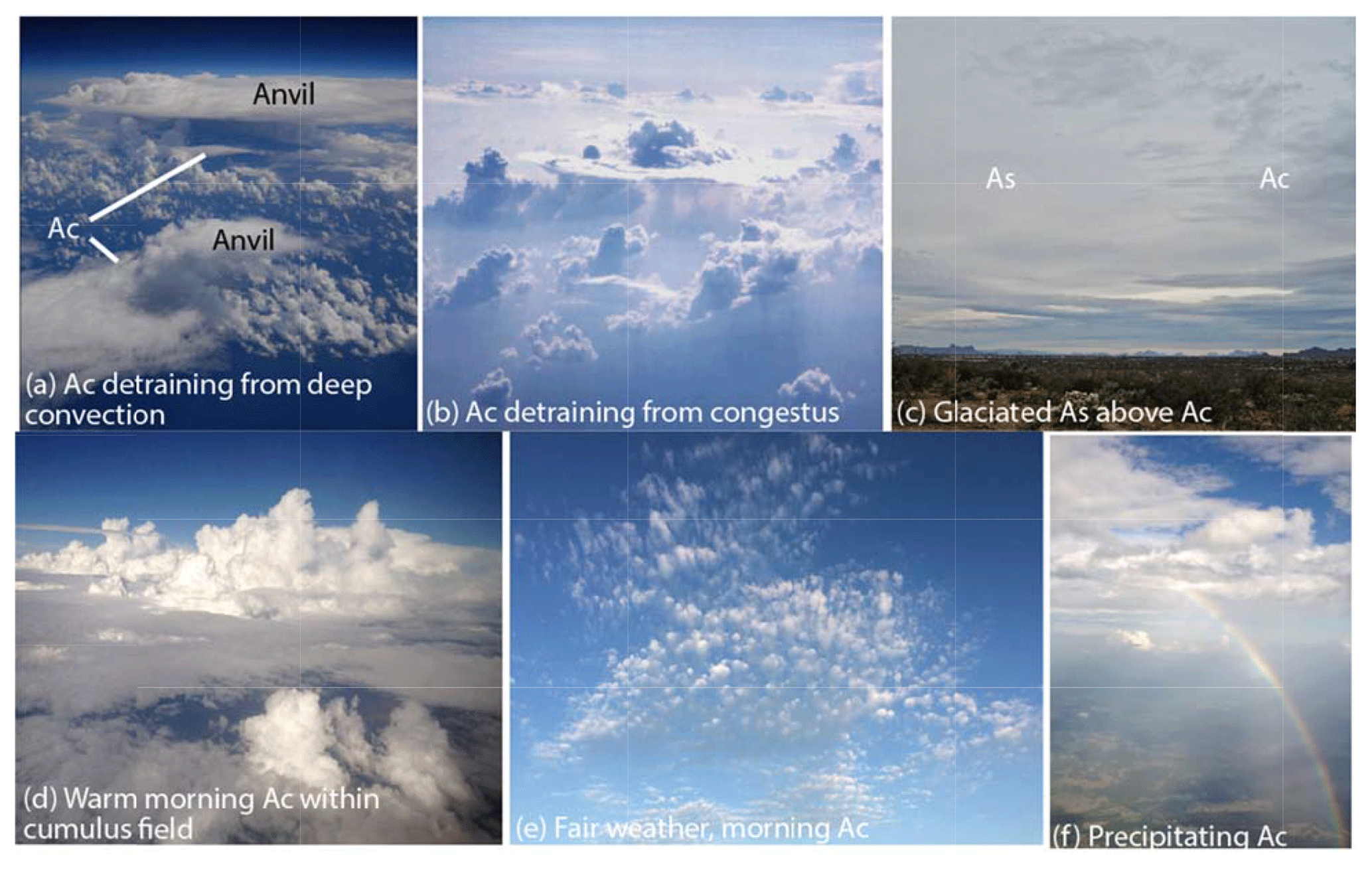
Figure 1 Cloud photographs of Ac and As characteristics. (a) Image from the NASA ER-2 showing Ac shelf clouds detraining from deep convection over the Gulf of Mexico during SEAC⁴RS; (b) Ac detraining from Cumulus congestus in a field of biomass burning smoke over Brazil (Reid et al., 1999); (c) mixed field of As above Ac clouds during a convectively active period in Arizona; (d) warm Ac clouds over developing cumulus field over west Texas during SEAC⁴RS ; (e) morning fair weather Ac field over Monterey, CA; (f) precipitating thin Ac clouds over central Texas during SEAC⁴RS. (Photo credit: (a) Donald S. Broce, NASA; (b, c) Arthur L. Rangno, enhanced for contrast; (d–f): Jeffrey S. Reid.)

Ac clouds are prevalent in many forms such as castellanus, an indicator of midlevel instability; mountain wave lenticularis; and translucidus (or colloquially mackerel sky). One class of Ac clouds, colloquially referred to as shelf clouds, is caused in part by detrainment at midlevel from deep convection (Fig. 1a; see Johnson et al., 1999; Yasunga et al., 2006). These clouds are not assigned their own genus in the International Cloud Atlas (Cohen, 2017), but the generic Ac is recognized as associated with the spreading of convective elements at a stable layer.

We know that Ac cloud prevalence is strongly associated with convective environments, such as in association with the Madden–Julian Oscillation (Riley et al., 2011). Ac shelves often form at 0 ^∘C from deep convection or in association with midlevel inversions (e.g., Johnson et al., 1996, 1999; Riihimaki et al., 2012). A primary production mechanism is thought to be related to the formation of 0 ^∘C stable layers initiated by the melting of falling frozen hydrometeors and enhanced condensation to compensate for the cooling (Posselt et al., 2008; Yasunga et al., 2008). Hydrometeor evaporation processes discussed in Posselt et al. (2008) have likewise been hypothesized to help form the inversion. This results in a thin cloud feature forming just below the inversion. Shelf-like Ac from towering cumulus (TCu) are also frequently observed (Fig. 1b) and may be related to the detrainment of overshooting tops around regional 0 ^∘C stable layers formed by surrounding convection (Johnson et al., 1996), or upper-level subsidence. Combined Ac and associated Alto stratus (As) coverage can be high in convectively active regions (Fig. 1c). Ac can also form overnight from the residual PBL and then burn off during the day (Fig. 1d; Reid et al., 2017; Wood et al., 2018) or during fair weather conditions just ahead of more active weather (Fig. 1e). Ac formation by mesoscale lifting is also common. Although sometimes geometrically thin with low liquid water contents, Ac can generate copious virga (Fig. 1f).

Compared to other cloud species, the relationship between LMFT aerosol layers and Ac clouds has a small literature base. The largest fraction of papers relate to lidar observations of smoke and dust as ice nuclei (IN) in mixed-phase alto clouds (e.g., Hogan et al., 2003; Sassen et al., 2003; Wang et al., 2004; Sassen and Khvorostyanov, 2008; Ansmann et al., 2009; Wang et al., 2015). However, cloud condensation nuclei (CCN) budgets for these cloud types have not been studied in detail with in situ observations, particularly for entirely liquid clouds. The complex mixed-phase nature of alto-level clouds and stratiform precipitation coupled with their thin nature and low updraft velocities (Schmidt et al., 2014) likely lead to sensitivity to even small perturbation in CCN concentration (Reid et al., 1999; Schmidt et al., 2015; Wang et al., 2015). Clouds can serve as aqueous-phase reactors of gas and aerosol particle species, even hosting nucleation events (Hegg et al., 1991), while evaporating droplets and precipitation leave residual aerosol particles. Given that Ac clouds are observed to have a strong impact in shortwave solar radiation (Sassen and Khvorostyanov, 2007), the hypotheses of Parungo et al. (1994) are worthy of consideration despite initial skepticism (e.g., Norris, 1999). Only now are the tools becoming available to quantitatively investigate further.

Observing the aerosol–Ac environment is challenging. The scarcity of data for alto-level aerosol layers in the convective regimes where Ac clouds often form, combined with the contextual or sampling biases inherent for the in situ observations of such layers and sun-synchronous polar-orbiting aerosol observations, obscures the true importance of LMFT aerosol layers in atmospheric aerosol life cycle and Ac cloud physics. An opportunity for study arose with the summer 2013 NASA Studies of Emissions and Atmospheric Composition, Clouds and Climate Coupling by Regional Surveys (SEAC⁴RS; Toon et al., 2016) field mission. For SEAC⁴RS, the NASA DC-8, NASA ER-2 and Spec Inc Learjet 25 aircraft were deployed along with ground assets including the University of Wisconsin Space Science and Engineering Center (SSEC) High Spectral Resolution Lidar (UW HSRL) to examine the aerosol and cloud environment of the summertime eastern United States (Toon et al., 2016; Reid et al., 2017). These observations allowed for comprehensive measurements of the structure and microphysical properties of local convectively generated LMFT aerosol layers.

SEAC⁴RS provided a valuable but complex dataset-especially in the vicinity of active convection. To simplify the analysis, this paper provides a case study of the covariability between aerosol layers and LMFT Ac clouds in convective environments using observations collected on 12 August 2013 (Fig. A1 in the Appendix). This day was chosen due to the isolated regional nature of the convection that occurred, as well as availability of ground-based lidar and airborne DC-8 sampling. This analysis will provide context for further exploration of the SEAC⁴RS datasets.

For this analysis we define Ac consistent with the WMO definition (Houze, 1993; WMO https://cloudatlas.wmo.int/clouds-definitions.html, last access: March 2018) of midaltitude (2–7 km) clouds that are (a) liquid or mixed phase and (b) decoupled from direct surface forcing. We begin with a brief description of datasets used in the remainder of the paper (Sect. 2). We then provide an overall narrative of the meteorological situation on 12 August (Sect. 3) followed by an analysis of the UW HSRL (Sect. 4) and data collected from a nearby storm by the DC-8 (Sect. 5). In the paper's discussion (Sect. 6), we explore commonalities in the two datasets and further explore hypotheses of LMFT layer characteristics, their origins and relationships to Ac clouds to set the stage for subsequent papers. A final summary and conclusions are presented in Sect. 7.

2 Data and methods

The analysis presented here centers around the 12 August 2013 SEAC⁴RS airborne research flight based out of Ellington Field, Houston, TX (Toon et al., 2016). The Ellington deployment for the SEAC⁴RS mission was conducted from 12 August to 23 September with three research aircraft (NASA DC-8, NASA ER-2, SPEC Learjet 25), an extensive ground network including Aerosol Robotic Network (AERONET) sun photometers (Holben et al., 1998; Toon et al., 2016) and the deployment of the UW HSRL to Huntsville (Reid et al., 2017). Comprehensive descriptions of the field assets are provided in this section's cited papers; here we provide a short summary of datasets used in this analysis.

2.1 UW HSRL deployment to Huntsville

LMFT aerosol and cloud layers were monitored by a 532 nm UW HSRL system, deployed by the NASA Cloud-Aerosol Lidar and Infrared Pathfinder Satellite Observations (CALIPSO) science team to enhance monitoring at the Regional Atmospheric Profiling Center for Discovery (RAPCD) lidar facility at the University of Alabama in Huntsville (UAH) National Space Sciences Technology Center (NSSTC) building (−34.725^∘ N; 86.645^∘ W), from 18 June to 4 November 2013. The RAPCD facility is located on the western side of the city of Huntsville at an elevation of ∼220 m. Including building height, the lidar transmitter was situated at 230 m a.m.s.l. (above mean sea level). Overall the local terrain is flat, with the exception of a line of hills protruding an additional 200–350 m and located 10–15 km to the east and southeast. The UW HSRL was hardened for continuous use and collected contiguous aerosol backscatter and depolarization data every 1 min at 30 m vertical resolution. The only significant notable outages were from 20 to 22 August and from 13 to 17 September. UW HSRL observations can be visualized and downloaded through the SSEC HSRL web page (http://hsrl.ssec.wisc.edu/, last access: February 2019).

The UW HSRL was able to extract the aerosol backscatter profile to very high fidelity. Unlike more common elastic backscatter lidar measurements that must deconvolve a combined molecular and aerosol signal in an inversion, HSRL systems can separate a line broadened molecular backscatter signal from the total backscatter signal via a notch filter (Eloranta et al., 2005, 2014; Hair et al., 2008). The difference is used to calculate aerosol backscatter. For this deployment the UW HSRL performed with a precision in aerosol backscatter of better than 10⁻⁷ (m sr)⁻¹ for a 1 min average and 10⁻⁸ (m sr)⁻¹ for 15 min averages. In comparison, Rayleigh backscattering is $\mathrm{1}\times {\mathrm{10}}^{-\mathrm{6}}$ (m sr)⁻¹ at 4 km, and $\mathrm{5}\times {\mathrm{10}}^{-\mathrm{7}}$ (m sr)⁻¹ at 10 km. Thus, at 15 min averaging, precision is likewise better than 1 % to 5 % of Rayleigh backscatter. This very high sensitivity to aerosol scattering is a result of the combination of the aforementioned HSRL ability to separate the molecular from aerosol scattering, the large signal-to-noise (SNR) ratio of the instrument, and the high solar background rejection during daytime observations. It is challenging to make a direct comparison of the ground-based HSRL to CALIOP given the very different viewing and sampling combined with the highly variable SNR of CALIOP between day and night observations. The NASA Langley airborne HSRL was used to validate the CALIPSO aerosol retrievals (Burton et al., 2013) and found that only 13 % of the layers identified as smoke by the Langley HSRL were correctly identified by CALIOP using the V3 CALIOP products. The UW HSRL, being a stationary ground-based system, provides even greater sensitivity to the aerosol backscatter as it can dwell over the same location for a long period of time.

By calculating the slope of the returned molecular scattering, aerosol light extinction can be directly calculated. However, as described in Reid et al. (2017), there are several caveats. First, there must be significant enough signal to calculate the slope; in this instrument, extinction must be greater than 0.1 km⁻¹. Second, one must account for an overlap correction in the near field, accounting for the fact that the telescope is not fully in focus until a range of about 4.5 km from the system. The signal below the 4.5 km level appeared to vary in time, sometimes hourly, during the daytime. Consequently, for the altitude range we will study here, it is best to rely on aerosol backscatter. Noting that extinction is simply the aerosol backscatter times the lidar ratio (S_a), here we assume a lidar ratio of 55 sr⁻¹ as a baseline (Reid et al., 2017). Expected deviations from this baseline are discussed in the results and discussion sections.

In addition to the lidar, several other deployments to the UAH site are used here. Most notably, UAH was a Southeast American Consortium for Intensive Ozonesonde Network Study (SEACIONS) release site (http://croc.gsfc.nasa.gov/seacions/, last access: 17 December 2018). Forty sondes were released between 6 August and 21 September 2013, at 18:00–19:00 Z/13:00–14:00 CDT to coincide with early afternoon boundary layer conditions, midflight airborne activity and the NASA A-Train overpass. For 12 August 2013, the release time was 13:42 CDT and is used here for situational awareness and the mapping of cloud and aerosol layers to their temperatures.

2.2 The SEAC⁴RS DC-8 operations

The DC-8 conducted 24 flights with patterns that covered the western United States through the southeastern United States (SEUS) and into the Gulf of Mexico. Flight patterns often included three primary relevant components. (1) A ∼100 km curtain wall pattern with multiple flat flight levels from 5 km to the near surface to collect free troposphere, entrainment zone, cloud base and near-surface samples; (2) saw toothed transits to monitor the lower troposphere for chemistry applications; and (3) spirals in the vicinity of developing deep convection. Such components are visible in this day's flight (Fig. A1). Flight restrictions in the vicinity of Huntsville prevented vertical profiles directly over the UW HSRL. Nevertheless, the DC-8 had ample opportunity to sample the SEUS LMFT environment, in particular for the case of 12 August 2013 examined here.

The DC-8 hosted its most comprehensive instrument suite ever to support the chemistry, convection, radiation, and upper troposphere and lower stratosphere (UTLS) science goals and customers. However, for the particular test case and application examined here, there are several caveats worth noting. While the ground-based UW HSRL can detect the fine aerosol structure in convective environments and in the vicinity of Ac clouds, generating in situ observations to correspond to this structure is difficult. At flight speeds of ∼120–150 m s⁻¹, the DC-8 is only in a detrainment patch for a few seconds, causing difficulty in differentiating small-scale aerosol features. Further, the massive payload of the DC-8, although comprehensive, also leads to functional problems as instrument calibration, maintenance and scanning cycles were not synchronized. Shattering effects of liquid cloud droplets and ice further disrupted the sampling of the very near cloud environment. Thus, one cannot retrieve the full complement of all data for an entire profile or flight component, let alone for individual features that the DC-8 might observe for less than 10 s. While the DC-8 carried a lidar system of its own, stand-off distances from the aperture and cloud heterogeneity prevented its use in this particular analysis. Nevertheless, the DC-8 hosted a number of instruments that can provide a valuable view of the overall aerosol and cloud structure in the 12 August 2013 convective environment which can be coupled with the lidar observations. These key instruments are listed as follows.

State variables. Navigation was derived from DC-8 housekeeping variables. Pressure, temperature and winds were measured by the NASA Ames Meteorological Measurement System (MMS, Scott et al., 1990). Moisture-related variables were derived from the NASA Langley Diode Laser Hygrometer (DLH, Podolske et al., 2003; Livingston et al., 2008).

Aerosol physical and optical properties. Baseline aerosol number, size and optical properties were derived from the Langley Aerosol Research Group Experiment (https://airbornescience.nasa.gov/instrument/LARGE, last access: 17 August 2019, Ziemba et al., 2013; Corr et al., 2016) instrument set, which included continuously sampling nephelometer, condensation nuclei counters (CNCs), and optical particle encounters. The LARGE package monitored aerosol particles from ultrafine condensation nuclei (CN) to an inlet cut point of ∼3.5 µm, and units reflect volumetric scaling to a standard temperature and pressure of 20 ^∘C and 1013 hPa. To prevent any possible cloud water or precipitation shattering effects on the aerosol instruments, CN, nephelometer, and laser aerosol spectrometer (LAS) data were heavily cloud screened with data points removed for one second before the arrival and two seconds after the exit of any cloud with LWC >0.005 g m⁻³.

Aerosol chemistry. Aerosol chemistry was evaluated using data from the CU aircraft HR-AMS (Canagaratna et al., 2007; Dunlea et al., 2009; http://cires1.colorado.edu/jimenez-group/wiki/index.php/FAQ_for_AMS_Data_Users, last access: March 2018) that reports the composition of submicron nonrefractory particles. Reported O ∕ C and OA ∕ OC ratios from this instrument were derived using the updated calibration of Canagaratna et al. (2015). Unlike single-particle instruments, the AMS is fairly insensitive to inlet artifacts during cloud penetration. Data points that were flagged as being potentially impacted by such artifacts (by monitoring excess water and/or zinc in the aerosol mass spectrum) were removed prior to analysis.

Cloud properties. Cloud detection properties were derived from the SPEC microphysics package (e.g., Lawson, 2011; Lawson et al., 2001, 2006, 2010), in particular the Fast Cloud Droplet Probe (FCDP) which provided the core cloud liquid water product and the 2D-2 for ice identification.

Gas chemistry. While the DC-8 carried comprehensive gas chemistry instrumentation, for this overview case study we rely on CO from the Differential Absorption CO Measurement (DACOM, Sachse et al., 1987; McMillan et al., 2011), CO₂ from non-dispersive IR analyzer measurements (Vay et al., 2011) and SO₂ from mass spectroscopy (Kim et al., 2007).

2.3 Ancillary datasets

In the analysis presented here multiple datasets were examined but for brevity are not shown in detail here. Regional meteorology was diagnosed through a combination of NEXRAD radar (NOAA NWS, 1991), GOES-13 geostationary and MODIS satellite datasets, and models. Baseline meteorology was provided by a Coupled Ocean/Atmosphere Mesoscale Prediction System (COAMPS^®) analysis including NEXRAD precipitation and wind assimilation (Zhao et al., 2008; Lu et al., 2011). Operational MODIS aerosol (MOD/MYD04, Levy et al., 2013) and cloud (MOD/MYD 06, Platnick et al., 2003, 2017) were also used. Geostationary imagery was generated at Space Sciences and Engineering Center with cloud products generated by Minnis et al. (2008). Regional aerosol concentrations were taken from Southeastern Aerosol Research and Characterization (SEARCH, Edgerton et al., 2015) and Chemical Speciation Network (CSN), as well as AERONET (Holben et al., 1998) sun photometer data. Back trajectories were utilized from HYSPLIT (Stein et al., 2015).

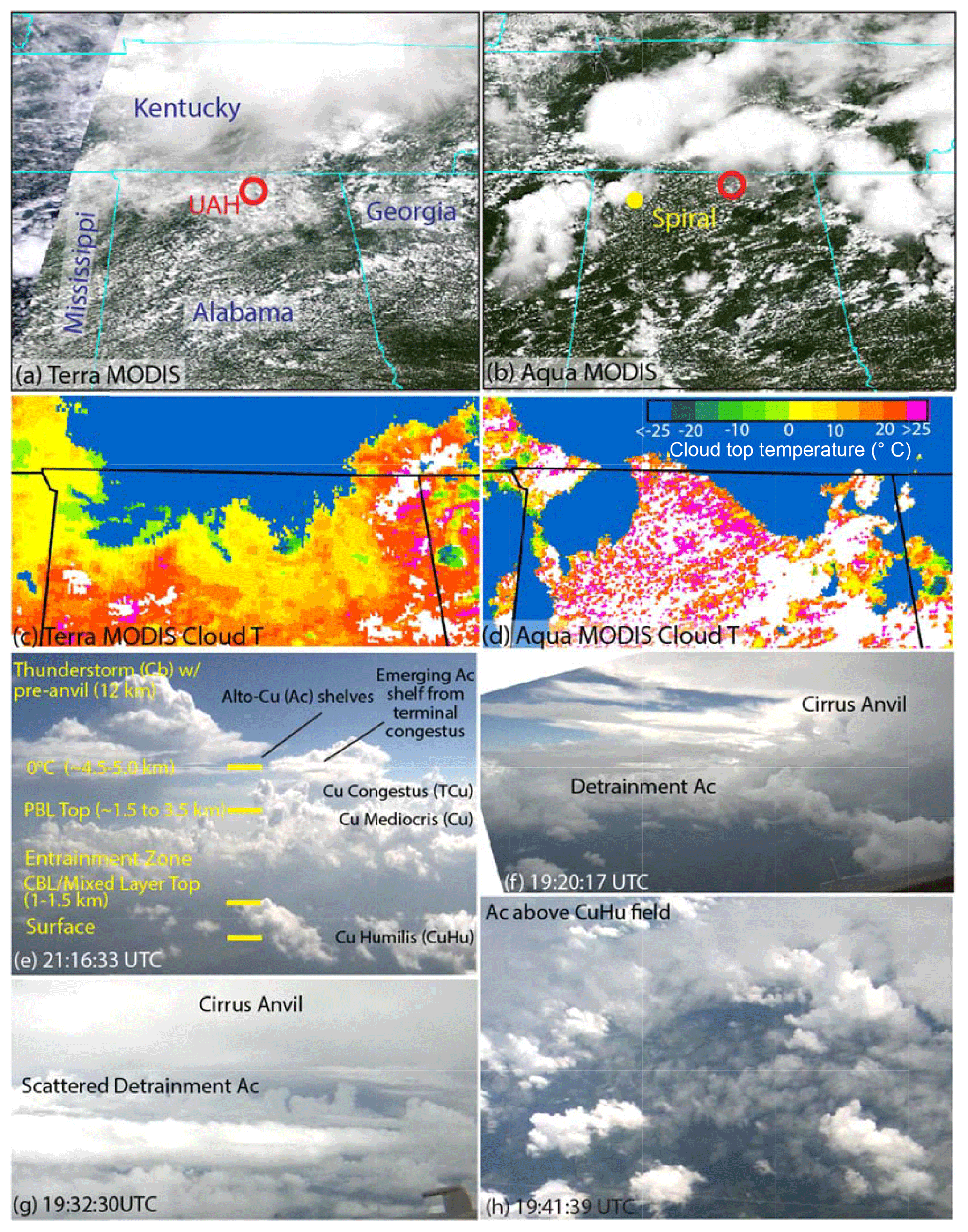
Figure 2 MODIS (a) Terra (16:00 UTC) and (b) Aqua (19:14 UTC) images, with markers indicating the location of the UAH lidar site (red) and DC-8 spiral (yellow) for 12 August 2013. Corresponding MYD06 cloud top temperatures zoomed onto northern Alabama are provided in (c) and (d). Also included are annotated camera images from the NASA DC-8 demonstrating cloud type (e) image just after profile components end; (f) forward images as the DC-8 was about to enter a detrainment Ac at 4.4 km; (g) forward image of the DC-8 while sampling the 6.5 km aerosol layer; (h) nadir images of an Ac detrainment shelf exiting a Cb over a field of Cu. Image from NASA Worldview (https://worldview.earthdata.nasa.gov/, last access: 17 August 2019).

3 Regional context for the 12 August case

Analysis of the 12 August 2013 case study is greatly aided by context provided by a regional weather analysis guided by satellite and lidar observations. A more detailed meteorological analysis is provided in Appendix A. In short, on 12 August 2103 the SEUS was in a fair weather summertime convective regime, with copious small convective, congestus and isolated Cbs. Images of the cloud field from MODIS and on-aircraft photography are provided in Fig. 2 (including MOD/MYD cloud top temperatures). Corresponding afternoon radiosonde sounding at UAH are also provided in Fig. 3 (release 18:40 GMT; 13:40 local CDT time) with (a) temperature and dew point, (b) water vapor mixing ratio and (c) wind speed and direction. The diurnal pattern of convection is also provided in NEXRAD composite radar images taken throughout the day, which are provided in Fig. A2.

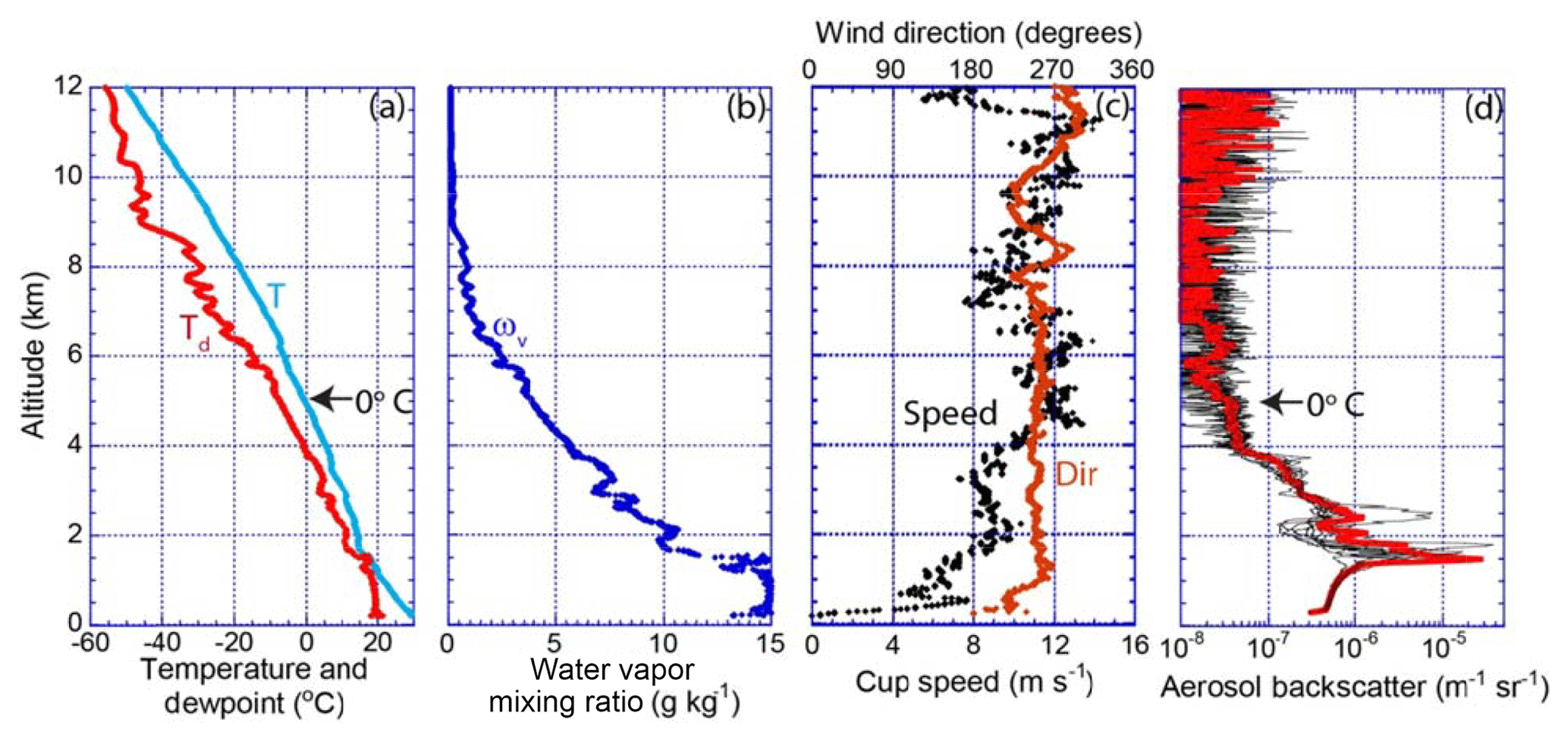
Figure 3 SEACIONS radiosonde release on 12 August 2013 18:40 Z/13:40 CDT at Huntsville (altitude in m.s.l., 200 m greater than ground level). (a) Temperature and dew point; (b) water vapor mixing ratio; (c) wind cup speed and direction; (d) 5 min aerosol backscatter profiles from the UW HSRL at Huntsville for the 2 h after the radiosonde release, with the mean value in red.

By daybreak on 12 August, the convection of the previous day had largely subsided over Alabama (Fig. A2b and c). Northern Alabama experienced developing Cu and Ac, with cirrus (Ci) intermixed to the north in the morning hours (e.g., Terra MODIS 16:00 UTC, Fig. 2a and c) in association with the stationary front. Continuing southward, cloud fractions outside of the cirrus and Ac domain ranged from 70 % to 90 %. Just before the Terra overpass, isolated convection was initiated throughout the region, including several cells north and east of the UAH site. By early afternoon (Aqua MODIS 19:14 UTC, Figs. 2b and A2d and e), isolated precipitating cells were widespread across the region. At the same time, cloud fractions diminished significantly, with a notable reduction in midlevel Ac (yellow to light-green colors). Low-level cloud fractions diminished up to ∼60 %, but there were larger numbers of isolated and higher-topped TCu.

Of note here is the large area of optically thin ∼0 ^∘C clouds, presumably melting level Ac, extended southward from the more convectively active regions to the northwest at the Terra overpass. MODIS cloud retrievals suggest the associated Ac clouds were in the 3 to −3 ^∘C range, with effective radius values on the order of 8–10 µm and liquid water paths of ∼10–30 g m⁻³. However, inspection of the RGB images shows these clouds as semitransparent and it is unclear as to what the retrievals are sensitive to. The implications of this observation are elaborated on further in the discussion section.

Using the DC-8 forward-looking cameras during its flight on 12 August, ∼21:16 UTC, allows us to categorize the cloud types and heights of the cloud bases and cloud tops of the observed clouds at the time of the flight (Fig. 2e–h). Forward camera images of the environment very near the deepest convection are provided in Fig. 2f and g, respectively, with a final nadir image of the Ac field departing the Cb in Fig. 2h. TCu and Cbs were more isolated, relative to the Ac, forming in association with the remnant outflow boundaries from previous storms rather than in organized and sustained lines. Clearly visible in Fig. 2e is a cloud base delineating the mixed layer and the PBL entrainment zone at ∼1.5 km, corresponding well to the UAH sounding. This entrainment zone was populated by Cumulus humilis (CuHu) to Cu with tops based on the DC-8 DIAL HSRL in the 1.5–3.8 km a.g.l. (above ground level) range, functionally defining the top of the PBL. Larger Cu occasionally rose to as high as 4.5–5 km, or to roughly the 0 ^∘C level (or ∼5 km from the sounding, but as shown later as low as 4.6 km from the DC-8). TCu rose to 6–6.5 km, with isolated Cb tops at 12 km. Between the PBL top and the Cb anvils, layers of Ac clouds were prevalent. Some of these Ac clouds are related to midlevel detrainment from Cbs, whereas others are clearly emanating near the tops of TCu (e.g., Fig. 2f–h). Near-surface haze was also visible, with Aqua MODIS and AERONET reporting 550 nm aerosol optical depth (AOD) on the order of 0.25–0.35. Reported PM_2.5 was on the order of ∼8 µg m⁻³.

At the time of the early afternoon UAH radiosonde release, the sounding was typical for the area for a moderately unstable convective meteorological regime (Fig. 3), with the mixed layer and top inversion at 1500 m m.s.l. (1280 a.g.l.; Fig. 3a). Water vapor mixing ratio (Fig. 3b) was constant, as expected in the mixed layer, falling off rapidly with altitude above, and with small perturbations associated with temperature inversions. Winds were near constant at 250^∘ above the mixed layer, with steady increases to 12 m s⁻¹ at the 0 ^∘C melting level at 4.6 km providing only a modest amount of shear (Fig. 3c). Derived convective available potential energy (CAPE) from the UAH sounding was 1650 J kg⁻¹ (moderate instability), consistent with TCu to isolated Cb development. As discussed in the next section, the corresponding HSRL aerosol backscatter profiles for this release are in Fig. 3d.

Figure 4 Example lidar data for 12 August 2013. UW HSRL aerosol (a) backscatter and (b) depolarization from the surface to 14 km a.g.l. Listed are cloud types; phenomenon; and, from a 13:30 radiosonde release, key temperature isopleths. Also shown in (c) are liquid and ice cloud bases (solid) from the ground-based HSRL and liquid and cloud tops from GOES-13 (open). To convert from a.g.l. to m.s.l., subtract 220 m.

4 Results I: HSRL observations

While the above analysis qualitatively describes the nature of the cloud fields, the time series of aerosol backscatter and depolarization from the UW HSRL from 12 August, 00:00 UTC, through 13 August, 09:00 UTC (Fig. 4a and b, respectively), provides a quantitative representation of the intricate regional aerosol and cloud environment. Lidar data in Fig. 4 were averaged over 1 min intervals and over 30 m vertical layers and represent a time period that extended from the local sunset of 11 August through daybreak on 13 August. Included for reference are ceilometer-like cloud bases identified in the lidar data for liquid and ice clouds (Fig. 4c), with associated geostationary derived cloud tops. Recall key temperature, water vapor and wind levels included from the 12 August, 18:40 UTC, SEACIONS radiosonde release are further provided in Fig. 3a, b and c respectively and HSRL aerosol backscatter profiles within ±3 h in Fig. 3d. Temperature levels from this release are included in Fig. 4. Likewise, mean and individual aerosol backscatter profiles (every other 5 min average, 30 m resolution) are included in Fig. 3d for the 2 h after the sounding when the DC-8 was sampling northern Alabama.

The meteorology and aerosol profiles depicted in Fig. 4 show considerable fine-scale structure in cloud and aerosol features. Considered in concert with Fig. 3, Fig. 4 indicates this day is consistent with the description of the convective environment in Reid et al. (2017) for a similar 8 August 2013 case. Thus, the description of the overall nature of the aerosol environment does not need to be repeated here in detail, other than to identify the key layers. During the 2 h period surrounding the 18:40 UTC radiosonde release, (1) there is a mixed layer that extends from the surface to 1500 m a.g.l., identifiable by a constant water vapor mixing ratio (ω_v; Fig. 3b) and an increase in aerosol backscatter in height due to increases in relative humidity (RH) with height and hence hygroscopic growth (Figs. 3d and 4a); (2) above the mixed layer inversion lies the entrainment zone, including visible detrainment layers; (3) as discussed above and shown in Fig. 2e, the top of the PBL is ambiguous as it relates to cloud tops in a heterogeneous cloud field, but a clear reduction in aerosol backscatter is visible at 4 km, likely related to the tops of regional Cu; (4) a second drop in aerosol backscatter occurs at the 0 ^∘C melting level (∼4.5 to 5.0 km from regional soundings and the DC-8) on this day; (5) a final aerosol layer between 6 and 7 km which, as we discuss later, may be associated with cloud top detrainment from TCu. Assuming a baseline S_a=55 sr⁻¹ as derived by Reid et al. (2017) an aerosol backscatter of $\mathrm{1}\times {\mathrm{10}}^{-\mathrm{6}}$ (m sr)⁻¹ (yellow) is equivalent to an aerosol extinction of 0.055 km⁻¹. Integration of aerosol backscatter from the surface to 10 km for cloud-free periods with this lidar ratio suggests a 532 nm AOD of ∼0.17, dropping to 0.12 later in the day, identical to AERONET.

Figure 5 Aerosol backscatter for inset boxes as labeled in Fig. 4 of key altocumulus and aerosol features for the 12 August 2013 case. Included is aerosol depolarization where ice is prevalent including an inset in (a) and a depolarization in (f) corresponding to (e). All times are UTC.

Moving from the sonde release to the whole period shown in Fig. 4, the above description of the thermodynamic and aerosol state of the atmosphere holds for the day. Clouds and precipitation are clearly visible in the aerosol backscatter color scales as dark red (backscatter $>{\mathrm{10}}^{-\mathrm{4}}$ (m sr)⁻¹. Comparing aerosol backscatter with depolarization for the whole column (Fig. 4a, b), clouds dominated by ice are easily identifiable from liquid by depolarization values above 40 % (Sassen, 1991), although as discussed later in association with DC-8 observations, low depolarization does not exclude the presence of ice. Large liquid water drops can also depolarize the lidar signal and signify heavy precipitation, and they are thus annotated on Fig. 4a. Yellow highlight boxes of interesting cloud and aerosol phenomena are marked on Fig. 4a, with corresponding enhancements of key features in Fig. 5 derived from 10 s, 7.5 m data. Finally, certain cloud types are annotated, including Ac, Sc and Ci.

Expanding the analysis to include the early evening of the previous day, radar and satellite data (Figs. A2 and A3) indicated multiple Cbs at various states of life cycle were within 15–30 km of the UAH lidar site. Consequently, cirrus (notable by its high depolarization) were detected through 12 August 2013 07:00 UTC (02:00 CDT) with bases for virga or ice falls between 8 to 13 km, or −35 to −57 ^∘C. Given that homogenous ice nucleation can begin at −37 ^∘C, except in the most extreme conditions, at these temperatures water tends to be ice (Pruppacher and Klett, 1997; Campbell et al., 2015). Virga is observed at cloud bases at ∼4.5 and ∼8.5 km m.s.l., highlighted in Fig. 5a. Using depolarization, we can see the upper cloud at 8.5 km and −25 ^∘C has ice virga emanating from supercooled liquid water in classic Ac fashion. The cloud base at 4.5 km and 0 ^∘C is entirely liquid by lidar observation, although we expect mixed-phase processes at work above where the lidar beam was attenuated. This behavior in combination with local NEXRAD radar data suggests this lower cloud feature is stratiform precipitation from the anvil of a decaying system.

In the morning of 12 August until just after daybreak (sunrise ∼13:05 Z; 06:05 CDT), a strong aerosol return was visible centered on the 1–1.5 km m.s.l./0.8–1.3 km a.g.l. range, likely a residual layer from the previous day's PBL mixed layer (ML, to 1.2 km) or entrainment zone (EZ, ∼2.5 km). This residual layer may have been transported from the east but also may be a result of nighttime cooling and enhanced relative humidity and particle hygroscopicity. Morning Stratocumulus are embedded in this layer and small liquid water Ac cloud returns are also visible in the morning (inset box Fig. 5b), at 05:00 UTC at ∼6 km (−7 ^∘C), 10:00 UTC 4 km (5 ^∘C), with the strongest returns at the 4.7 km 0 ^∘C melting level at 12:00 UTC. These clouds likely originate from convective detrainment of water vapor, such as from melting level detrainment of convection (e.g., Fig. 1a, b) or from the tops of TCu clouds, sustained by cloud cooling. Associated with these clouds are clearly visible individual pockets of aerosol particles on the order of a few hundred meters high and 15–30 min in duration. With backscatter returns on the order of 1 to $\mathrm{5}\times {\mathrm{10}}^{-\mathrm{7}}$ (m sr)⁻¹, such features are <5 % of Rayleigh backscatter and demonstrate the Ac are embedded in larger aerosol features. At wind speeds of 5–10 m s⁻¹, these pockets are between ∼5 and 20 km wide.

In the early morning hours, local time, tenuous clouds are also observed at 1 km within the ML residual layer, likely nighttime radiatively driven Sc. By local daybreak, CuHu begin to more systematically form at ∼1 km due to solar heating at the surface, with cloud base heights increasing to 1.5 km as the ML and PBL develop throughout the morning to early afternoon LST (inset Fig. 5c). Clouds also formed at daybreak at 1.5 km inside a PBL residual aerosol layer. At this height, above the CuHu, these clouds are decoupled from surface forcing and are optically thin, suggesting they are Ac, even though they share their initial formation physics with Sc earlier in the day. More interestingly, a second Ac deck formed shortly thereafter, with 2–2.5 km m.s.l. bases that increased in height with time through the morning to a maximum height of 3.7 km (5.5 ^∘C), collinear with the depth of the mixed layer. These are highlighted in inset box Fig. 5c. Based on geostationary imagery, and as demonstrated in the comparison of Fig. 2a–b, these clouds evaporated at noon local time, presumably under solar radiation. This situation is similar to the case of Fig. 1f. Interestingly, aerosol layers between the PBL clouds and the Ac are also visible, forming in the late morning at ∼15:30 UTC, and increasing with height with the developing PBL and the Ac clouds above. Cirrus also begins to advect over the site by afternoon, largely detraining from thunderstorms to the north and west (Fig. A2b).

By 23:00 UTC, a mature-phase Cb spawned by the outflow of the storm sampled by the NASA DC-8 4–5 h earlier arrived at Huntsville, bringing showers to moderately heavy rain. The remnants of the storm extend through the next day, producing Ac visible from 13 August, 00:00 to 03:00 UTC, between the 4.5 km melting level and 7 km (−12 ^∘C) and (Fig. 5d). These clouds, most likely local in origin, are often categorized as convective debris Ac by the forecasting and aviation community – an indicator of multilevel detrainment in the convective environment. An aerosol layer exists to approximately the 4.5 km 0 ^∘C melting level capped by Ac. Additional Ac exist above these embedded in faint but clearly visible aerosol layer features. Unlike the aerosol pockets earlier in the day, these features are much more limited in extent, no more than 200–300 m in depth.

As the PBL collapses during the evening, it leaves a 1 km a.g.l. residual layer not unlike those present a day earlier. A final set of light showers from a decaying system occurs after the early morning of 13 August at 07:30 UTC (Fig. 5e). With another clear melting level visible in the depolarization data, this is likely residual stratiform precipitation like at the beginning of the time series. Similar to the beginning of the time series, ice precipitation from supercooled liquid water clouds was also present.

5 Results II: DC-8 observations of an 12 August 2013 storm outflow

The HSRL gives an excellent depiction of the overall aerosol backscatter and cloud phase over the course of the day, but it lacks the ability to provide microphysical and chemistry information on the aerosol particles themselves. For this purpose, we utilize measurements on the DC-8 that flew in the region on this day. The flight pattern on 12 August included a curtain wall over the Gulf of Mexico, sawtooth transit to a curtain wall over northeastern Alabama and more sawtooth patterns to a spiral on the downwind side of deep convection developing over the northwestern corner of Alabama. This last maneuver in northern Alabama is marked on Fig. 2b and provided the day's only complete tropospheric profile. Being on the downwind side of the storm's trajectory, this profile also gives a snapshot of the aerosol environment detraining from an isolated storm being fed by a polluted boundary layer. As the storms later passed over Huntsville, observations collected by the DC-8 also provided context for the UW HSRL lidar observations described in Sect. 4. Figure 2 includes forward and nadir images of the overall environment. However, the most representative depiction of the midday to early afternoon environment is provided in Fig. 2e, taken at 10 km altitude just as the DC-8 started its return from sampling the storm. The region had a deck of CuHu and Cu with bases at 1.4 km m.s.l./∼1.2 km a.g.l., delineating the PBL's mixed layer from its entrainment zone. As mentioned, the PBL top was more ambiguous and is functionally defined by the tops of these clouds at ∼2.5–4 km (e.g., Fig. 2a). TCu were observed, overshooting above the 0 ^∘C level, as were scattered Cbs with tops at ∼12–13 km. Ac were prevalent on the horizon, detraining both from overshooting TCu and midlevel of Cbs.

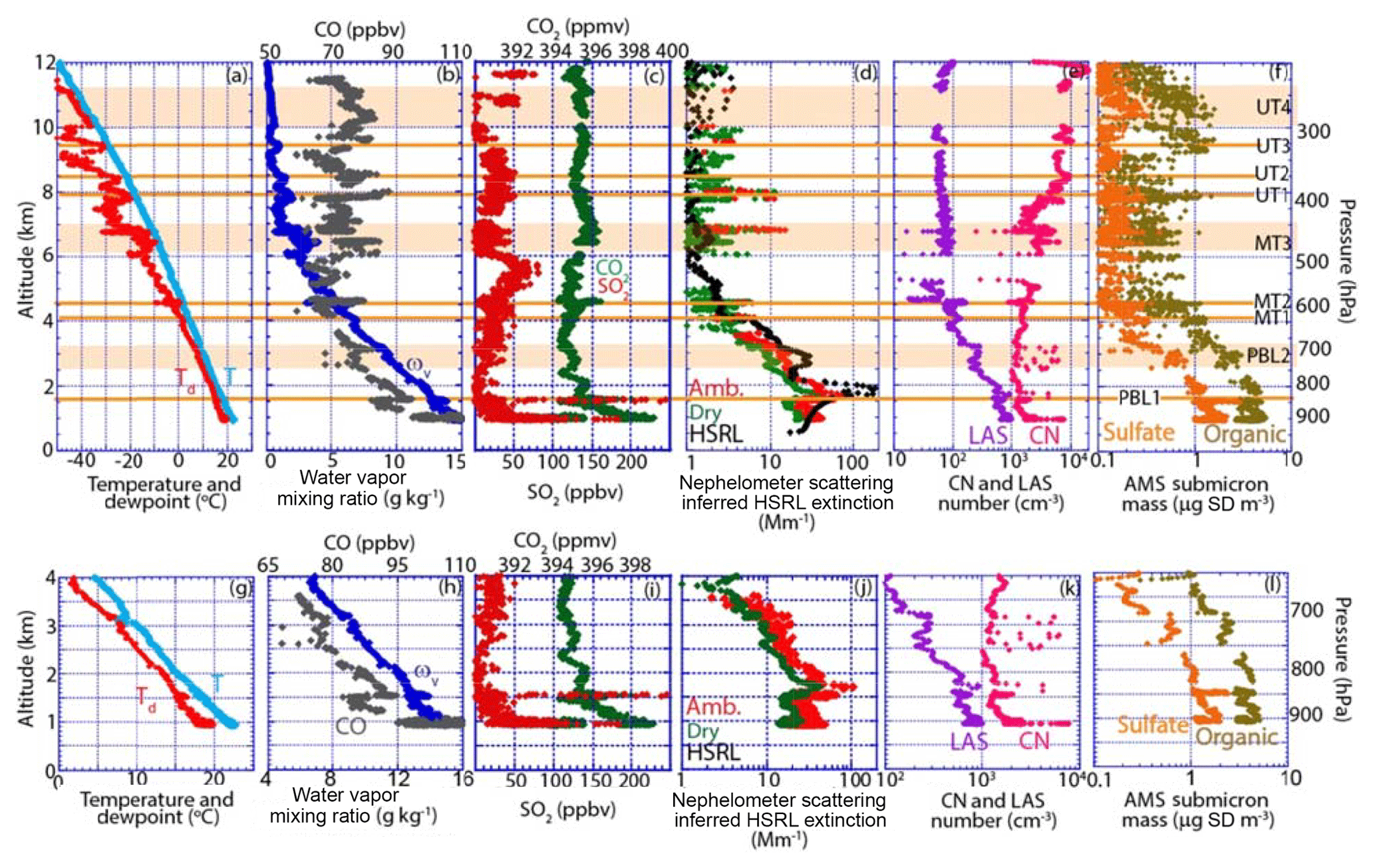
Figure 6 DC-8 aircraft spiral sounding data initiated on 12 August 2013 at 19:10:30 UTC on the downwind side of a thunderstorm over northwest Alabama. Altitudes are relative to mean sea level, ∼300 m higher than a.g.l. Included is (a) temperature and dew point; (b) water vapor mixing ratio (ω_v) and CO; (c) CO₂ and SO₂; (d) DC-8 total ambient and a fine dry 550 nm nephelometer with the ground-based UW-HSRL-derived extinction (lidar ratio =55 sr⁻¹) at Huntsville Al; (e) number concentration from laser aerosol spectrometer (LAS, d_p>0.1 µm) and condensation nuclei (CN, d_p>10 nm); (f) aerosol mass spectrometer organic materials and sulfate. Key moisture and aerosol layers as discussed in the text are marked as orange lines or bands. (g–f)  same as (a–e) expanded in the vertical to enhance PBL feature readability, and the legends are equivalent.

Profile variables collected by probes on the DC-8 during the spiral initiated at 19:10:30 are provided in Fig. 6. Included are (a) temperature and dew point (of liquid water) and tracer species (b) ω_v and CO and (c) CO₂ and SO₂. To depict particle scattering (d) provides the DC-8 total ambient 550 nm light scattering and a parallel dry light scattering for fine particles (<1 µm). For context also included on Fig. 6d is the inferred light extinction derived from the UW HSRL by assuming a lidar ratio of 55 sr⁻¹. The period of averaging for the HSRL data is 19:00–21:00 UTC, or essentially from the start of the profile until just before the storms passed overhead. Total particle counts from the LAS and CN counters are plotted on Fig. 6f. To prevent any possible cloud water or precipitation shattering effects on the aerosol instruments, CN, nephelometer and LAS data were heavily cloud screened with data points removed for one second before the arrival and two seconds after the exit of any cloud with LWC >0.005 g m⁻³. Finally University of Colorado aerosol mass spectrometer organic material and sulfate are provided in Fig. 5f. Only under very heavy ice content conditions do AMS data need to be expunged from the profile. To reduce noise, a 5 s boxcar average was applied to the particle counter and AMS data. Also to improve readability of PBL features, similar plots from 0–4 km are likewise included as Fig. 6g–l respectively.

Table 1 Key physical attributes (mean and ± standard deviation) of detrainment layers observed from the 12 August 2017 thunderstorm. Included are altitude in mean sea level (∼300 m higher than above ground level), temperature and water vapor mixing ratio (ω_v), carbon monoxide (CO), carbon dioxide (CO₂), sulfur dioxide (SO₂) laser aerosol spectrometer (LAS) number and volume at STP, 550 nm dry light scattering for particles less than 1 µm, and aerosol mass spectrometer (AMS) organic carbon (OC) and sulfate at STP. Layers are defined as shown in Fig. 6.

^a Mixed layer properties were taken as a 5 s average just before assent. ^b CO instrument was in a calibration cycle for part of this layer. ^c Upper troposphere. N/A: not available.

The DC-8 profile depicts the intricate layering behavior throughout the free troposphere in a fashion consistent with the UW HSRL backscatter. As expected, the temperature profile is largely moist adiabatic ∼6 ^∘C km⁻¹, indicating an atmosphere that has been modified by convective processes. Moist layers, well depicted in the dew point sounding when it converges with temperature, often coincided with minor temperature inversions. For reference, these layers associated with dew point depressions <2 ^∘C are labeled on Fig. 6 as lines or, for three deeper layers, shaded bands. Characteristics of these layers are also provided in Table 1, and Fig. A4 provides images taken from the DC-8's forward video for visual context of the environment being sampled. As expected, moist layers coincided with increases in ω_v. However, these layers also strongly coincided with increases in other trace species such as CO and dry aerosol concentration. In the following subsection, we provide a narrative starting with layers influenced by PBL detrainment (PBL layers 1 and 2; Sect. 5.1) followed by upper free troposphere detrainment by the Cb (UT layers 1–4; Sect. 5.2). Emphasis will then be placed on the nature of aerosol and Ac layers in the middle free troposphere (MT layers 1–3; Sect. 5.3). Finally we will examine composition and particle properties between these layers (Sect. 5.4).

5.1 PBL detrainment layers

Our first area of examination is of detraining aerosol layers associated with the development of the PBL, with clouds ranging from CuHu to Cu and the occasional congestus. This baseline PBL environment is described in detail in Reid et al. (2017) and is the subject of a subsequent paper on particle transformation and inhomogeneity within the PBL. Here, we consider a few specific aspects of the DC-8 dataset to aid in overall profile interpretation, and also in the analysis of covariability among aerosol, water vapor and Ac cloud formation in the middle troposphere.

To begin we examine the nature of the PBL's mixed layer as this is the source of the atmospheric constituents being convectively lofted. However, the observation of the PBL's mixed layer profile at the bottom of the profile is contrary to what one would expect. Most notably, gas tracers such as ω_v CO, CO₂, SO₂ and particle properties are not constant with height near the bottom of the profile. Based on forward video (Fig. A3a), the spiral was initiated below cloud base, and thus we are confident this sample is indeed in the mixed layer. Indeed, there was a strong gradient in ω_v on approach to the spiral; in fact, isolated showers were seen across the horizon. It is therefore likely that the mixed layer is influenced by regional gradients – a recurring problem with profiling with large and fast moving research aircraft. These gradients are good indicators of significant spatial variability of atmospheric constituents in the mixed layer. Using a single point at the top of the mixed layer just before ascent as a baseline (Table 1), ω_v and CO were at a maximum of the profile at 15.5 g kg⁻¹ and 110 ppbv, respectively. CO₂ was elevated to ∼190 ppbv and SO₂ 225 pptv. CN was at 2300 cm⁻³, and LAS had a volume concentration of 2.8 µm³ cm⁻³ for an index of refraction of polystyrene spheres (n=1.55), consistent with AMS concentration of particulate organic matter and sulfate of 4.2 and 1.5 µg m⁻³, respectively. The ratio of increased light scattering due to hygroscopic growth from 20 % to 80 % RH was 1.62, typical of the region (Wonaschuetz et al., 2012).

Within the nearest level to the surface (PBL layer 1 in Fig. 6, ∼1.6 km m.s.l., 1.4 km a.g.l.) is a clear aerosol enhancement just at and above the mixed layer top which we diagnosed at ∼1.5 km through a combination of water vapor and temperature and visual inspection of cloud base from the forward video (Fig. A4). An enhancement is expected in ambient scattering at the top of the mixed layer due to the increases in humidity (80 % at the middle mixed layer and reaching ∼90 % between clouds) with height in the mixed layer coupled with aerosol hygroscopicity. But just above the mixed layer there is an increase in CO, CO₂, dry aerosol mass, number, CN and scattering. SO₂ values were exceptionally high, reaching off the plot scale to 300 pptv, indeed suggesting strong compositional spatial inhomogeneity in the region. This, like the mixed layer variables, might be a combination of an aliased signal but also is influenced by detrainment from the Cu clearly present (Fig. A3b). At Huntsville at the same time as the DC-8 spiral, the unaliased HSRL profile showed classic increased aerosol backscatter (and presumed extinction) to a maximum at a level of 2 km m.s.l., indicating the top of the mixed layer and cloud base slightly higher than the spiral location. PBL layer 1 is made up of simultaneous spikes within ω_v, CO, dry light scattering, LAS and CN concentrations, and AMS sulfate as the DC-8 passed through the top of the mixed layer and into the level of the lowest cloud bases (∼1.5 km a.g.l.; Fig. A4b). Also was a likewise spike in SO₂. Although not shown, NO₂ spiked to mixed layer levels (tens → hundreds of ppbv), with a minor dip in ozone. (40 →37 ppbv). This enchantment is presumably through the detrainment of mixed layer air via the fair weather cumulus. Dramatic increases in CN and sulfate in particular suggest that this layer potentially hosted secondary particle mass production via detrainment from nearby shallow clouds (e.g., Wonashuetz et al., 2012). Although RH values were on the order of 85 %–90 %, both the probe data and visual inspection of the video data show this peak is not associated with any form of cloud contamination. Ultimately, evidence suggests that this layer is detrainment of mixed layer air from small cumulus. Even though this location near the Tennessee River hosts some sporadic industry on its shores, the nature of the tracers, such as water vapor and CO, demonstrates this layer was convectively transported from above the mixed layer by small Cu. Recent studies suggest that the oxidation of SO₂ to SO₄⁼ in such clouds can be extremely fast (e.g., Loughner et al., 2011; Eck et al., 2014; Wang et al., 2016).

The second layer analyzed, PBL layer 2, was much deeper than the first, at 2.5–3.2 m.s.l. (Fig. A3c). This layer can be classified as the upper portion of the PBL entrainment zone, where air is actively mixing with the free troposphere above via detrainment from cumulus. The ω_v is enhanced and, between clouds, relative humidity ranged from 80 % to 90 %. At times enhancements existed in LAS particle number and in AMS sulfate and OC. Spikes in CN concentration reached 10 000 cm⁻³, likely a product of convective boundary layer precursor emissions receiving high actinic flux not only directly from the sun, but also reflected from nearby clouds (e.g., Radke and Hobbs, 1991; Perry and Hobbs, 1994; Clarke et al., 1998). As then expected, SO₂ was diminished. During the DC-8's transit of this layer there was a 15 s Cu penetration that included significant precipitation, although this period is expunged from the aerosol particle counter record in Fig. 6. In the middle of this cloud, CO reached 80 ppbv, indicating convective lofting of mixed layer air. It is this cloud that we believe developed into the CB sampled. At the time of this first penetration, from visual inspection, the cloud top could not have been more than ∼1 km above the aircraft (Fig. A4c), consistent with it not being picked up with NEXRAD.

The PBL layer 2 detrainment environment is discussed in detail in Reid et al. (2017), and owing to convective pumping and cloud processing of mixed layer air and high relative humidity it contributes significantly to regional AOD variability. Sometimes described as cloud halo effects to explain covariability in cloud fraction and AOD, this PBL layer 2 is actually a widespread detrainment-induced layer (Reid et al., 2017). This layer was visible not only on the DC-8 nephelometer and AMS data, but is also coincident with a strong aerosol return from the Huntsville lidar, some ∼100 km to the west. Notably, the top of this layer coincides with the lifting aerosol layer topped by Ac clouds in UW HSRL (Figs. 1f, 3a, 4c) and serves as a potential boundary between the PBL and free troposphere.

5.2 Upper free troposphere

Moving from PBL-influenced aerosol layers, we now briefly examine the region dominated by convective outflow from the anvil, diagnosed as detrainment in association with ice. This altitude domain is largely outside the scope of this paper and will be discussed in detail in other SEAC⁴RS papers. Nevertheless, for completeness a brief description is provided here. Like the top of the PBL, the bottom of the cirrus anvil outflow layer is ambiguous. From Fig. 4 and in particular Fig. 5a, it is clear that liquid water could exist as high as 8.5 km, or $\sim -\mathrm{21}$ ^∘C, although ice was clearly nucleating and falling below this liquid water. The first full ice layers were experienced by the DC-8 at 8 and 8.4 km (UT1 and 2, Fig. A3g, h), followed by a second cirrus cloud (UT2), a third at 9.4 km (UT3; Fig. A3i) and finally a deep cirrus penetration from 10 to 11 km (UT4; Fig. A3j). Because cloud particles in these layers were entirely made of ice, with ice water content approaching 1 g m⁻³, aerosol size and scattering data are not available; although prominent peaks in CO, sulfate and particulate organic matter are found at each level indicating convective pumping and detrainment. SO₂ showed varied positive and negative correlations with these layers, suggesting perhaps varying influences of the background and directly detrained air masses. From an aerosol point of view, it is obvious that significant enhancements in particle mass and number exist on either side of the cirrus layer. Notably the boundaries of these layers were enriched in organics relative to sulfates, and CN >10 nm concentrations were on the order of 10 000–20 000 cm⁻³, particularly above 9.5 km. Indeed, observations suggest that deep convection is highly efficient at transporting boundary layer air through to the anvil (Yang et al., 2015).

5.3 Middle free tropospheric layers

The focus of this paper is on the middle tropospheric detrainment layers, bounded below by the primary PBL detrainment layer and its associated Ac clouds and above by the anvil cirrus, both described above. Within the middle troposphere there were numerous perturbations in water vapor, trace gas and aerosol features. In particular, three coincident water vapor, CO and aerosol layers were observed in the DC-8 spiral, clearly associated with liquid water clouds (MT layers 1, 2 and 3; Fig. A4d, e, f). Starting from the bottom of the free troposphere and working upwards, a slight inversion at 4.1 km delineated a rather minor water vapor and aerosol layer (Fig. 6 MT1; Fig. A4d), which, like layer PBL2, spanned both the DC-8 profile and the UW HSRL lidar at Huntsville. The inversion associated with this layer was a 200 m deep area having a near-constant temperature of 3.4 ^∘C. Visual inspection of video data suggests this level was associated with the maximum heights of the larger Cu and likely represents the very top of convective pumping by larger boundary layer clouds (Fig. A4d). Such an interpretation is also consistent with this layer delineating a drop in aerosol light scattering and mass which has likely detrained from these larger clouds. Yet coincident with this inversion is a small spike in particle number, as measured by the CN counter. The similarity of this layer to PBL2 is noticeable, even if ejections are more sporadic than the smaller and more numerous cumulus clouds in the region that define PBL2. These layers may be isolated, or be associated with a more organized region, but they nevertheless show the lofting of mixed layer air into the free troposphere. Indeed, this layer reminds us that in convective environments the physical top of the PBL is difficult to define; the boundary between the cloud tops and the free troposphere is variable.

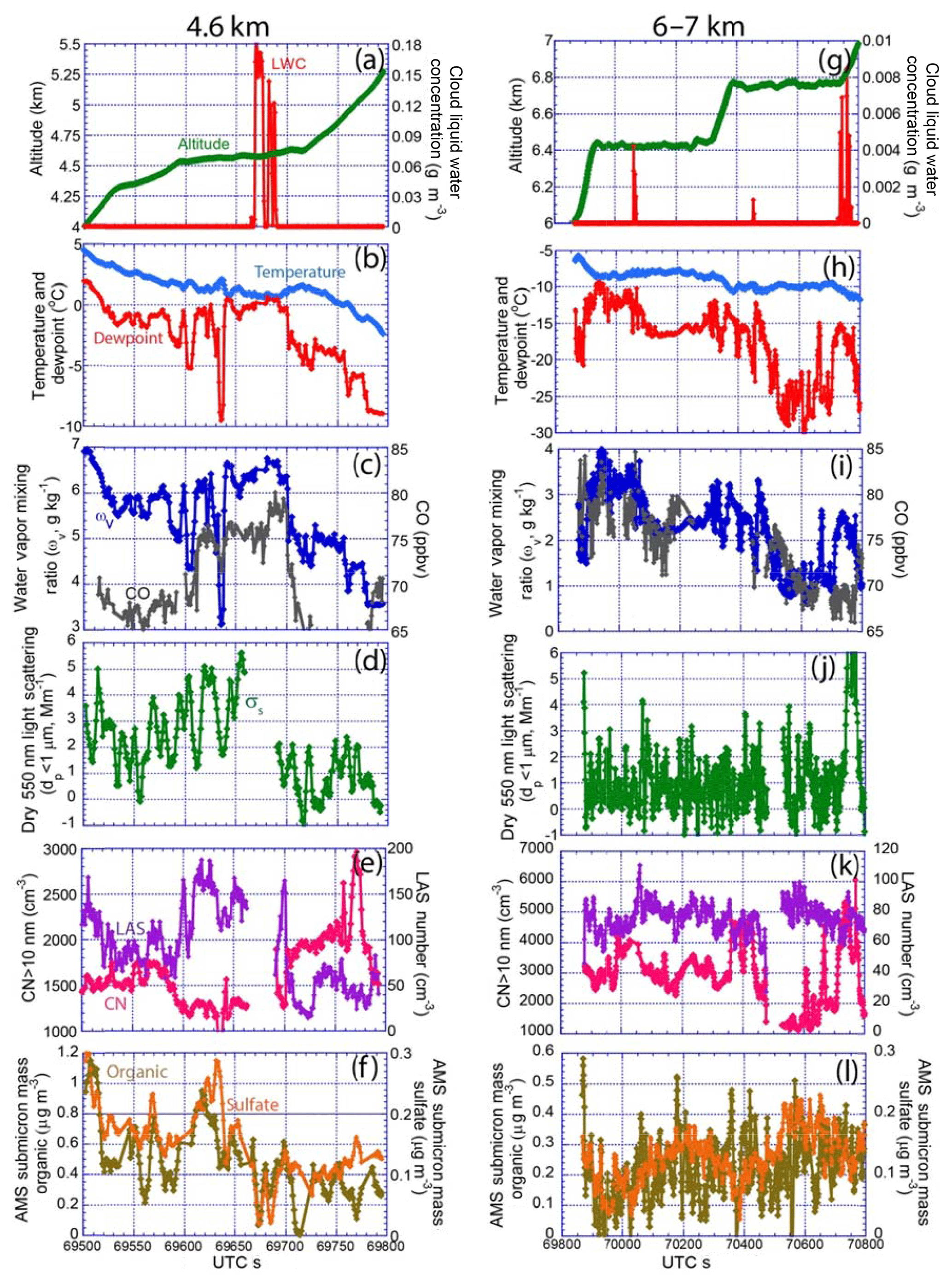
Figure 7 Time series of key meteorology, cloud and aerosol properties entering a detrainment shelf cloud on 12 August 2014. The legends for the graphs on the left are the same for graphs on the right.

Special attention is paid here to the next two layers (MT2 and MT3) where significant perturbations to trace gas and aerosol loadings were associated with thin Ac cloud decks. Within MT2, a strong aerosol return was present at 4.6 km, associated with a shelf cloud deck at ∼0.5 ^∘C detraining from the sampled Cb (Fig. 2d and A4e). Most notably, the MT2 layer also showed the strongest positive perturbations for ω_v, CO, CO₂ and a minimum in SO₂. This suggests that air from this layer was largely from the boundary layer with its SO₂ scavenged. MT3 contained a deeper layer of isolated Ac clouds from ∼6 to 7 km (−6 to −12 ^∘C; Fig. A3f). These layers are similar in nature to layers observed throughout the day at Huntsville (e.g., Fig. 5b, d). Detailed time series of data as the DC-8 passed through these two layers are presented in Fig. 7.

MT2 at 4.6 km was targeted for direct penetration by the DC-8 because it represented a classic melting level Ac detrainment shelf commonly observed around the middle of Cbs (e.g., Fig. 1a; Johnson et al., 1996; Posselt et al., 2008). The DC-8 approached the cloud from the side at a slow climb rate (∼1 m s⁻¹) and flattened out for Ac cloud sampling, followed by a more accelerated climb (Fig. 7a). Consequently, the DC-8 captured the environment below and to the side of the Ac deck, as well as the Ac deck itself. Given the air speed of ∼156 m s⁻¹, the 50 s time series for this aerosol and cloud layer spans ∼8 km. On approach, water vapor, CO, dry light scattering and aerosol mass species also increased in a layer perhaps only 200 m thick. Water vapor changed in a series of steps, suggesting coherent layers, including a very sharp drop in water vapor for only a few seconds just before cloud penetration, only to drop again on exit. The drop in ω_v and cloud liquid water was immediately below a 2 ^∘C magnitude temperature inversion.

Aerosol particle counts for d_p>0.1 µm (and particle volume, not shown) also increased on approach to the Ac. Total CN (d_p>10 nm) dropped precipitously, suggesting an overall shift in the background size distribution in an environment that disfavored nucleation. Cloud penetration lasted ∼20 s (∼3 km) and cloud liquid water contents ranged from 0.12 to 0.18 g m⁻³. Droplet effective radius from the cloud probes (not shown) was consistently in the 4.5–6 µm range, lower than the ∼8 µm values observed by Terra MODIS earlier in the day. Not surprisingly, with a cloud temperature of ∼1 ^∘C no ice was present. While aerosol number or size distributions are unavailable during cloud sampling due to inlet shattering, CO clearly peaked within 200 m of the altitude of the cloud. Yet, the AMS showed a decrease not only within the cloud but also just before cloud entry. As the DC-8 climbed up and away from the Ac deck, LAS particle counts and AMS OC and sulfate dropped, while CN returned to baseline levels and even spiked for a short period. Overall, MT2 observations match qualitatively what was seen in the HSRL data, with the cloud resting on the top of the aerosol layer.

While MT2 was associated with a thin detrainment shelf, layer MT3 was representative of a much deeper layer of convective detrainment, spanning the 6–7 km level. Like MT2, there was enhancement of ω_v, CO₂, and CO, as well as a reduction in SO₂. These layers can be visualized in the Huntsville HSRL data in Fig. 5b and d. Sampling of this layer was in the form of steps (Fig. 7g). Throughout this layer, ω_v and relative humidity varied in such a way that this overarching layer is most likely an agglomerate of many layers. The existence of several thin layers at various heights may result from detrainment at the tops of terminal congestus with termina at different levels (Moser and Lasher-Trapp, 2017). Consequently, very faint Ac clouds were visible on the video (e.g., Fig. A4f), though there were few actual cloud penetrations. The clouds sampled had very meager liquid water contents (<0.01 g m⁻³) – barely clouds. Yet, these clouds were mixed phase with ice clearly visible in 2-D probe data at temperatures of −10^∘ C (Fig. A5 annuluses are also ice out of focus). Under some circumstances ice habits can be indicative of ice-forming temperatures. However, for these clouds, ice particle were over a millimeter in diameter and of irregular habit. There is some indication from column and hollow column habit, consistent with a local freezing at −10 ^∘C and low supersaturation. But without precise temperature histories this is largely conjecture. Such ice is not always noticeable in lidar data, as optics may be still dominated by spherical liquid droplets.

For most of MT3, ω_v and CO varied in concert. However, at the very top of the level, they quickly become anticorrelated – suggesting water vapor at this location is not being brought from the boundary layer. Instead, it may be from entrained air along the sides – perhaps along cloud edges air entraining in is the first to detrain out (Yeo and Romps, 2013). Aerosol data are not much more enlightening. Aerosol mass was rather steady and at reduced concentration than its lower-level counterparts. At the same time, spikes in aerosol counter and nephelometer data occurred near clouds and may just as easily be a result of a droplet shattering artifact rather than convective pumping.

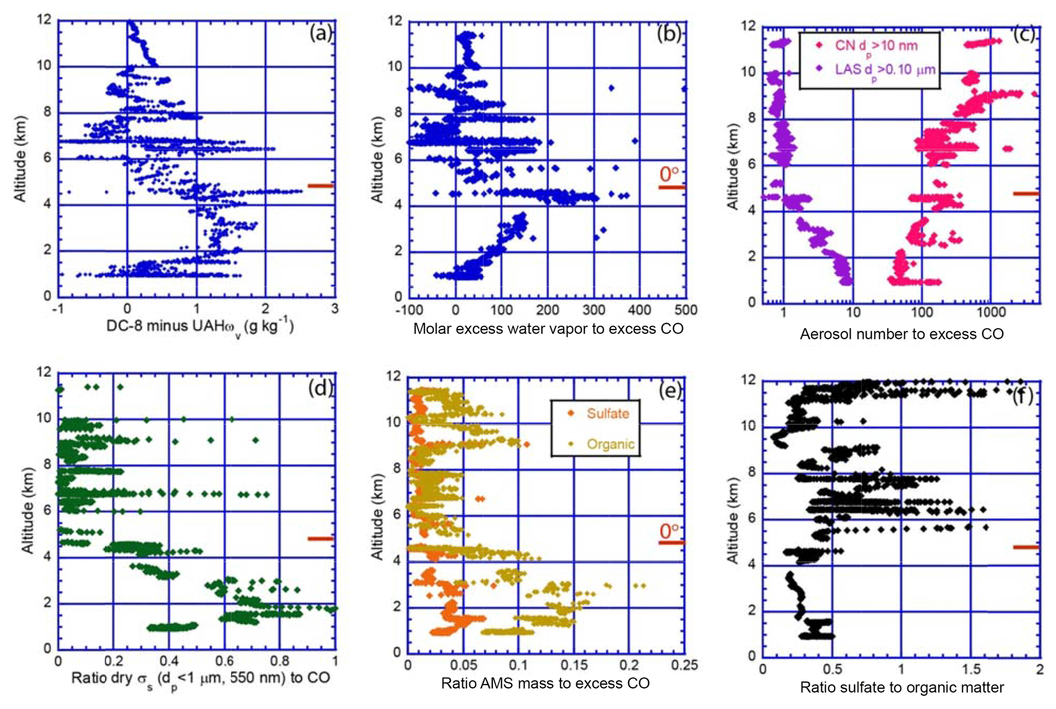
Figure 8 (a) Difference in water vapor mixing ratio between the DC-8 profile and the SEACONS 12 August 2013 radiosonde release at Huntsville, AL. Profiles of key constituents relative to excess CO including (b) excess water vapor to excess CO, (c) aerosol number, (d) dry light scattering, (e) organic carbon and sulfate to excess CO, and (f) ratio of sulfate to particulate organic matter.

5.4 Vertical profile aerosol chemistry and mass

Previous subsections in Sect. 5 describe the nature of individual detrainment layers. In this final subsection, we provide a closer examination of differences in their properties. If we conceptualize the environment as being influenced by shallow to deep injections of mixed layer air being convectively transported to the free troposphere by clouds entraining and detraining air along the way, it is best to start with reliable tracers such as CO. Figure 8 includes profiles of the ratio of aerosol number and mass to excess CO.

5.4.1 H₂O and CO

Paramount to all subsequent interpretation of the profile is the molar ratio of excess water vapor to CO. Whereas we can take background CO value of 60 ppbv (or any nearby value as long as we are consistent), water vapor is a bit more problematic. We derived excess water vapor by taking advantage of the deep convection horizontal scope of several hundred kilometers upwind of UAH. A background value was derived from the average mixed layer mixing ratio, followed by a fourth-order polynomial fit against pressure above the mixed layer (r²=0.99). The calculated excess ω_v between the DC-8 and UAH sounding is provided in Fig. 8a. As expected, ω_v is enhanced in the vicinity of convection, notably in the mixed layer, as well as individual PBL and midlevel detrainment layers, such as 3 km (PBL2), 4.6 km (MT2, 0 ^∘C) and 6–7 km (MT3). Water vapor is also more broadly enhanced in the upper troposphere layers (UT1–4).

Moving from establishing the background water vapor profile, we next consider how a parcel of air lofted into the PBL deviates from textbook descriptions during deep convection. If the parcel ascends without mixing, the water vapor mixing ratio is expected to decrease with altitude, as temperature decreases at the moist adiabatic lapse rate and water vapor is removed by condensation and precipitation. In contrast, CO is expected to remain constant over the timescale of convective ascent. In reality, the vertical profiles of both constituents are modified by entrainment–detrainment processes, and theory and numerical experiments indicate there are few truly undiluted parcels to be found anywhere in regions of shallow or deep convection (Zipser, 2003; Romps, 2010; Romps and Kuang, 2010). Parcels that ascend in a region near the core of convection (far from the cloud edge) may conserve CO and approximately follow a moist adiabat. Parcels closer to the cloud top and edge will undergo mixing with air that has originated from various levels inside and outside of the cloud, and they may reflect multiple entrainment–detrainment events (Yeo and Romps, 2013). The ratio of water vapor to CO concentration in undiluted ascent should be uniquely determined by the parcel's initial properties in the mixed layer, and departures from this ratio within the cloud reflect the action of mixing. Outside of the cloud, the situation is a bit more complicated. We expect water vapor content to decrease with height, and, if CO is well mixed, then the concentration will be constant with height. Increases in the ratio of water vapor to CO with height reflect the action of detrainment from convection, as water vapor decreases with height more rapidly than CO.

The 0 ^∘C melting level is further related to the air parcel characteristics. The molar profile of excess H₂O to CO ratio is provided in Fig. 8b, and throughout the lower troposphere the ratio increased to a maximum at the 0 ^∘C melting level. This increase reflects a more rapid decrease in CO with height relative to water vapor and is punctuated by two local maxima in the ratio at 1.5 and 3 km above the surface. Above the melting level, the ratio of H₂O to CO precipitously drops and then exhibits local maxima at 5 and 5.5 km.

Examining possible causes of the water vapor and CO ratio variability in the vertical above the 0 ^∘C melting level entails a closer examination of the impacts of detrainment on an air parcel. Detrainment of air from convection results in local increases in both water vapor and CO; however, water vapor content in detrained air will be greater than CO due to evaporation of cloud condensate. The general increase in the water-vapor-to-CO ratio indicates the repeated action of entrainment–detrainment and evaporation of cloud condensate around developing cumulus clouds, while local maxima in the water-vapor-to-CO ratio reflect the action of enhanced detrainment at specific levels – in this case, the tops of CuHu and Cu at 1.5 and 3 km, respectively. Detraining air from congestus and deep convection at the melting level provides the strongest local source of water vapor (direct and via evaporated cloud), and also the largest water-vapor-to-CO ratio.

Contrary to the spikes in water vapor content caused by detrainment, immediately above the melting layer, water vapor content is very low as this air originates in the middle and upper free troposphere (cf., Fig. 4 and Posselt et al., 2008). CO consistently remains relatively high, since CO is relatively well mixed in the middle and upper free troposphere (Fig. 5b). The near discontinuity in water vapor content in the vertical, coupled with relatively small changes in CO, result in the rapid decrease in the water-vapor-to-CO ratio above the melting layer. Relatively high CO concentrations in the air detrained at and below the melting layer can be seen in the profile of CO (Fig. 5b) and in the aerosol number to CO ratio maxima in Fig. 7b. Above the melting layer, such as in the 6–7 km region (MT #3) thin layers of high water-vapor-to-CO ratio are likely due to detrainment from Cumulus congestus clouds.

Figure 9 Laser aerosol spectrometer (a) number and (b) volume distributions of aerosol layers as a function of altitude. The legends for the two graphs are the same.

5.4.2 Aerosol mass

Moving to aerosol particle profiles, different aspects of convective transport reveal themselves. The ratio of LAS particle concentration (d_p>0.1 µm, representing the accumulation mode) and CN (d_p>10 nm, representing the nucleation mode) to CO is presented in Fig. 8c. Relative to CO, accumulation mode particles largely drop continuously in number from the surface to 0 ^∘C level. Positive perturbations exist within the PBL and LMFT aerosol layers as diagnosed in Fig. 6. At heights above the 0 ^∘C level, the accumulation mode to CO ratio stabilizes at lower concentrations with occasional layers. There is some difference in light scattering (Fig. 8d) and OC and sulfate from the AMS (Fig. 8e), where we find mass enhancement in the PBL detrainment zone.

Nucleation mode aerosol becomes more prominent with height owing to more intense solar radiation and a decrease in available accumulation mode surface area. Nucleation rates of particles from precursor detrainment from anvils can be rapid (Waddicor et al., 2012). Detrainment layers host strong positive and negative perturbations in CN count, which do not project significantly onto light scattering or mass. This is in contrast to the concentration of accumulation mode particles which do project strongly onto optical observables.

To explore variability in particle size distributions in the vertical, Fig. 9a and b provide LAS number and volume size distributions for key levels throughout the profile, which is consistent with what can be inferred from Fig. 8. Best fit baseline particle size distribution within the mixed layer suggest count median diameter (CMD) and volume median diameter (VMD) of 0.14 and 0.25 µm, respectively. At the first layer (PBL 1), dry particle size CMD and VMD increases to 0.16 and 0.28 µm, respectively, at the same time of increases in particle mass relative to CO. This is all consistent with secondary aerosol particle mass production on existing particles. After this point, we find a reversal in particle CMD and VMD with height. This is suggestive of precipitation scavenging of larger particles in larger clouds the deeper the detrainment. That is, particles that are detraining from smaller nonprecipitating clouds keep their secondary produced mass. However, these same aerosol particles that grow to larger sizes are more likely to be lost to droplet nucleation and scavenging. Nevertheless, significant aerosol mass from the boundary layer still is ejected in the anvil as evidenced in the 9–11 km altitude range in Fig. 8d and e.

5.4.3 OC and sulfate

The 0 ^∘C level is clearly a delineator in the sulfate-to-OC ratio (Fig. 8f). Near the surface the ratio of sulfate to OC is ∼0.4. In the first PBL detrainment layer (PBL1) there is a doubling of sulfate relative to CO. Such a mass increase relative to CO may be indicative of secondary aerosol production – and indeed sulfate peaks in this layer not only against CO, but also relative to OC (Fig. 7e, f). Particulate organic matter mass relative to CO peaks in PBL layer 2, but with a reduction in sulfate. Detrainment from this layer is associated with deeper clouds, including warm precipitating clouds in the immediate vicinity. Thus, sulfate particles may be preferentially scavenged.

The ratio of sulfate to OC further changes systematically through the profile, decreasing to a minimum just below 4 km. This, coupled with the decrease in accumulation mode number relative to CO, may be a further indicator of aerosol particle processing and scavenging in clouds. Indeed, the midtroposphere layers that show a reduction in SO₂ do see an increase in sulfate. Above 4 km, sulfate increases again, perhaps due to oxidation of residual interstitial or dissolved but unoxidized sulfur species in either Ac clouds or in the gas phase. This increase may also be related to the relative mass distribution within detraining cloud droplets. Sulfate mass fractions do appear to recover in the upper troposphere, perhaps due to homogenous nucleation of the small amount of SO₂ detraining from sublimating ice. However, we cannot exclude this high number of nucleation mode particles as being part of the regional background.

6 Discussion I: combining datasets and hypothesis development

The purpose of this paper is to demonstrate on a canonical day that aerosol layering characteristics in the free troposphere and PBL entrainment zone are delineated by cloud structure and its associated thermodynamic profile. Examination of this day leads to many questions about aerosol processes and potential impacts or feedbacks with understudied Ac clouds. To help the field progress, in this section we use the combined datasets from the UW HSRL and the DC-8 aircraft to formulate several hypotheses about Ac formation that need further attention by the community.

6.1 Hypothesis: Ac cloud's low liquid water and slow updraft velocities are susceptible to small changes in the CCN population

One of the most remarkable aspects of next-generation lidar systems such as the UW HSRL used here and the new Raman systems such as described in Schmidt et al. (2015) is their ability to observe intricate aerosol features at very low particle concentrations. Figures 3d, 4 and 5 demonstrate fine coherent structure of aerosol layers in the free troposphere that, in the past, were rarely quantified. Even with aerosol backscatter levels at or even under $<\mathrm{5}\times {\mathrm{10}}^{-\mathrm{8}}$ (m sr)⁻¹, or <5 % of Rayleigh backscatter, aerosol layers of only a 100 to a few 100 m thickness are clearly visible. These thin aerosol layers can persist for hours, undergoing gravity wave undulations along with gradual changes in observed layer height at the meso- to synoptic scales. Ac are often associated with observed aerosol layers, and the clouds we observed had very low liquid water contents of a few tenths of a gram per cubic meter (g m⁻³) at most (e.g., Fig. 7). Drawing from parallels to Sc (e.g., Martin et al., 1994; Platnick and Twomey, 1994; Ackerman et al., 1995; to most recently Wood et al., 2018), or the very limited available measurements of such relationships for Ac in the field (e.g., Reid et al., 1999; Sassen and Wang, 2008; Schmidt et al., 2015), we would expect Ac clouds' low liquid water and slow updraft velocities to result in strong effective radius sensitivity to CCN populations. Indeed, Ac have characteristics very much like Sc (e.g., Heymsfield et al., 1991, 1993), and critical supersaturation can be reasonably well calculated for Sc and Ac (e.g., Snider et al., 2003; Guibert et al., 2003). Given the importance of solar radiation to cloud lifetime (e.g., Larson et al., 2001, 2006; Falk and Larson, 2007) it stands to reason that aerosol–Ac sensitivities can then project onto cloud reflectivity, cloud lifetime and consequently the local energy budget. Quantifying this balance of different terms influencing the parcel life cycle remains a challenge (e.g., Falk and Larson et al., 2007).

Nevertheless, global aerosol populations that have strongly varying signals regionally (e.g., Alfaro-Contreras et al., 2017) may result in large-scale trends in Ac cloud cover (e.g., hypotheses by Parungo et al., 1994) and reflectivity. However, estimating CCN concentration based on the regional aerosol loading is a difficult task. One is attempting to estimate the properties of a very thin aerosol layer with highly complex relationships to the boundary layer and regional convection using likewise complex microphysics in highly variable and at times weakly forced clouds. This is discussed further in Sect. 7.

6.2 Hypothesis: CN events can sustain and enhance CCN populations in Ac clouds

The impact of aerosol dynamics of the region must be considered when addressing a number of science questions. Aerosol backscatter is dominated by accumulation mode particles that, owing to their size, also make the best CCN. While there are copious CN, there are few particles in number of any appropriate size to behave as CCN (∼100 cm⁻³ or less in the LAS at altitudes above the 0 ^∘C level). Considering the proclivity of CN nucleation events, and the overall increasing numbers of CN at higher altitudes, the CCN versus optical detection relationship is complex, (e.g., Schmidt et al., 2015), especially if one considers homogenous nucleation and processing (e.g., Perry and Hobbs, 1994; Kazil et al., 2011). Enhancements in accumulation mode particles near Ac appear to be anticorrelated with CN for this case – likely due to available surface area for secondary mass production and or coagulation. At the same time, explosive nucleation events are visible and expected. This all leads to questions about layer flow dynamics in and around Ac and their associated aerosol layers and/or halos. Does the cycling of air through an Ac feed back into its own CCN budget? Does nonprecipitating cycling enhance particle size and hence CCN number for any given supersaturation? In precipitating Ac, where are replacement CCN coming from, and do nucleating CN ever offer a supply? Or, as a hypothesis, perhaps CN events can sustain and enhance CCN populations in Ac clouds. The null hypothesis would then be that CN are consumed in individual droplets and have little overall effect in clouds with such meager updraft velocities and super saturations. This topic in particular needs to be addressed in highly detailed modeling studies.

6.3 Hypothesis: at and below the melting level air is dominated by detrainment of boundary layer air, and above the melting level in the middle free troposphere air is more influenced by entrainment and detrainment along the cloud edges, but PBL air can be ejected through the anvil

This hypothesis or ones like it is related to the fundamental “plumbing” of convection and what fraction of air from which levels is transported where. Much of the combined Ac/aerosol environment rests on the nature of convective detrainment, and this detrainment phenomenon may give insight into cloud dynamics and transport. The updraft core is somewhat insulated from entrainment–detrainment processes, whereas parcels closer to the cloud top and edge will undergo mixing with air that has originated from various levels inside and outside of the cloud. Observations around clouds may reflect multiple entrainment–detrainment events (e.g., Yeo and Romps, 2013). The ratio of water vapor to CO concentration in undiluted ascent should be uniquely determined by the parcel's initial properties in the mixed layer, and departures from this ratio within the cloud reflect the action of mixing. Detraining air from deep convection at the melting level provides the strongest local source of water vapor (direct and via evaporated cloud), and also the largest water-vapor-to-CO ratio. We hypothesize that, up to and including the melting level, detrainment is dominated by boundary layer air, whereas above this level air is more influenced by entrainment and detrainment along the cloud tops and edges. Indeed, for the melting level shelf the significant combined enrichment of CO and CO₂ is perhaps the strongest evidence that air detraining from this level is from the boundary layer which presumably was from the core of the cell. It is noteworthy also that the Ac cloud observed on the DC-8 was not directly at 0 ^∘C, but rather 0.75 ^∘C, consistent with the formation of an inversion directly above it (e.g., Fig. 7b; T minimum not exactly at 0 ^∘C but rather at 0.5 ^∘C). These observations are in agreement with the simulations by Posselt et al. (2008) and Yasunaga et al. (2008), both of which were modeling studies that managed to form melting level clouds without any predefined environmental area of stability. Perturbations in temperature may be representative of large-scale vertical motions on the outside of the clouds, including downdrafts adjacent to regions of in-cloud upward motion. Schmidt et al. (2014) suggested that the heating–cooling differentials in the vicinity of altocumulus clouds can result in areas of mesoscale subsidence, further perturbing flow fields and presumably CCN intake into these clouds.

We leave open the possibility that depending on storm dynamics, parcels in the inner core of convection can be ejected into, and out of, the anvil. This overall structure, with PBL air at cloud tops and bottoms, with more entrainment–detrainment-dominated properties is supported in Fig. 8 where aerosol mass ratios to CO are given as well as an altitude dependence of sulfate to organic matter. So clearly different altitude ranges have strong relationships to cloud entrainment and detrainment processes and the overall convective structure. Models can certainly provide insight, but considerable thought must be given to verification.

7 Discussion II: water vapor, aerosol and altocumulus layer observations in the context of radiative balance and climate change

As elucidated in the introduction, Ac clouds do not garner the attention they deserve relative to their likely importance in the earth's radiation budget. This study demonstrates some of the key challenges that the community faces in establishing an Ac budget which may discourage investigation. Ac clouds challenge characterization by remote sensing in the following ways:

1. Ac clouds are prevalent in the early morning hours, as well as in the vicinity of convection, shielded by associated cirrus above and cumulus clouds below (Fig. 4). Thus, they are likely underrepresented in cloud climatologies based on satellites, particularly polar-orbiting ones such as on Terra, Aqua and JPSS.

2. Ac cloud layers have a significant open-celled structure, with very low liquid water contents and paths (e.g., Fig. A4). Combined with assumptions that underlie passive remote sensing, specifically that radiation is plane parallel and cloud fields are uniform in a pixel, remote sensing techniques are severely challenged by the fractus nature of these clouds. Indeed, in visible wavelengths we can see that the entire Ac deck is semitransparent (Figs. 1e, 2a, h).

3. Even under excellent viewing conditions, Ac clouds tend to exist at the same levels as large Cu (Fig. 1a, b, d). Thus, identification by single pixel IR techniques cannot distinguish between the two.

At the same time, the CCN populations for Ac decks are low in concentration and exist just below the cloud layer. Given the difficulties in modeling aerosol entrainment and entrainment processes, one might think that direct observation would be the most straightforward avenue of study. To provide aerosol microphysics information, an aircraft such as the DC-8 is required. But in the context of the aerosol structure highlighted in Fig. 5, aircraft sampling is highly aliased. This is compounded by the typical structure of a thin Ac deck above its associated thin aerosol layer. Broad sampling of the free troposphere would reveal only periodic collinear perturbations, and aircraft location relative to the rest of the fine aerosol structures would remain unknown. Even if the DC-8 aircraft were directly over the Huntsville site, interpretation of the data would be complicated by features such as gravity waves and halos around individual clouds. Based on the previous discussion in Sect. 6, we expect Ac to be highly sensitive to changes in CCN population, not only from the detrained layer, but also by layer nucleation and cloud processing. Compounding the remote sensing challenges of properly identifying Ac are the system's aerosol components. Clearly the proclivity of Ac to form in geometrically and optically thin detrainment layers defies current satellite remote sensing capabilities for layer detection. Layer penetration by aircraft is for only a few seconds and likely disrupts the cloud field.

Without a doubt, more in situ aircraft operations are needed, but they need be performed in conjunction with ground, airborne and space-based remote sensing, particularly lidars. Indeed, much of the Ac literature base surrounds lidar systems. While elastic backscatter systems certainly have merit, the low aerosol signal compared to the relatively bright Ac cloud presents a significant observational challenge. HSRL or Raman systems are needed in order to quantitatively derive quantitative aerosol backscatter and/or extinction around such features. Nevertheless, data from lidars are underdetermined. Aerosol backscatter and/or extinction, even spectrally resolved, are only semiquantitatively related to CCN concentrations.

The challenges the Ac system poses perhaps can be seen as an opportunity for the scientific community. Just as Ac clouds are likely underrepresented in some cloud studies, Ac clouds likewise disrupt other cloud studies. Certainly there are new satellite sensor concepts that can be considered, such as improved lidar and radar capabilities in association with the proposed NASA Aerosols and Clouds, Convection and Precipitation (ACCP) mission. But, these potentially new capabilities should be taken in the context of the existing tools. For example, any Ac-observing strategy should include the next generation of imagers, such as on GOES-16/17, Himawari-8, and Meteosat Third Generation (MTG). Higher-resolution imagers with infrared capabilities (e.g., Advanced Spaceborne Thermal Emission and Reflection Radiometer, ASTER; and Landsat-8) or near-infrared capabilities, such as Sentinel-2 Multispectral Instrument (MSI), are also excellent candidates for Ac characterization. In the meantime, dedicated airborne measurements with imagers and both aerosol and water vapor lidars can be brought to bear in short order. The Ac environment also provides currently untapped potential as a relatively closed system for high-resolution modeling and radiative transfer. Ac layers are less than a few 100 m thick and clearly have shear flows and overturning circulations associated with them (e.g., Fig. 5b). Study of Ac layers will, as such, likely require numerical simulations run with very high vertical and horizontal resolution. In addition, the potential susceptibility of Ac to changes in CCN requires the use of sophisticated aerosol-aware cloud microphysical schemes.

8 Conclusions

This paper presents 12 August 2013 as a case study from the SEAC⁴RS campaign that demonstrates Altocumulus cloud (Ac), aerosol and water vapor layering phenomena in a convective regime over the southeastern United States (SEUS). This day was chosen due to proximity of the DC-8 research aircraft to a High Spectral Resolution Lidar (HSRL) at Huntsville, AL. The HSRL gives period level perspective on Ac clouds and their observed aerosol halo to help interpret in situ DC-8 data. Analysis of the meteorology of the region on this day supported the assertion that aerosol was local to the SEUS and thus should be considered to be representative of regionally forced convective environments. A 33 h sample of lidar data was presented to demonstrate the diurnal cycle of cloud and aerosol features in this convective environment. The HSRL provided aerosol backscatter and precisions at or better than 5 % of Rayleigh backscatter and demonstrated extraordinarily fine aerosol features in the vicinity of altocumulus clouds formed in the outflow of deep convection. This day was in turn compared to a DC-8 profile conducted that afternoon on the downwind side of a developing storm providing in situ data on the middle free troposphere aerosol environment.

Aside from typical boundary layer development and cirrus outflow, numerous aerosol and Ac decks were identified, and many of these Ac produced ice virga. Ac formed at the top of the residual of the previous day's planetary boundary layer entrainment zone, where air was largely influenced by boundary layer cloud detrainment. This layer formed in the morning hours and increased in base altitude with the developing boundary layer below it. Such rising may be a result of mesoscale flows or cloud lofting.

Above the PBL-top Ac, several other combined aerosol–Ac–water-vapor layers were observed, including (1) a 4 km detrainment layer that we surmise is from the very tops of cumulus mediocris clouds, (2) layers just below 4.6 km/0 ^∘C melting level inversion (∼1.5 ^∘C inversion strength) representing deep convective detrainment shelves with air originating from the boundary layer, and (3) 6–7 km layers that appear to be consistent with detrainment from the tops of congestus clouds at the top of a layer of stability. From the HSRL and the DC-8 aerosol observations, Ac clouds were associated with clear aerosol halos, with Ac clouds on top. The intensity of aerosol backscatter associated with Ac cloud halos appeared to decrease with height, beyond what would be expected from adiabatic expansion. The lowest Ac clouds associated with PBL entrainment zone have larger returns associated with their proximity to the polluted PBL and large accumulation particle size, as well as hygroscopicity. However, middle free troposphere layers had markedly smaller accumulation mode sizes with height but higher CN counts and strong positive CO and CO₂. Aerosol layers above 0 ^∘C had the smaller accumulation mode sizes and highest CN concentrations. This is consistent with further cloud processing and scrubbing of detraining air at higher altitudes. Particle size and composition data suggest that detraining particles undergo aqueous-phase or microphysical transformations, while at the same time larger particles are being scavenged.

Examination of profiles suggest an excess of water vapor and aerosol particles relative to CO within and above the PBL entrainment zone to the melting level, and observations around clouds may reflect multiple entrainment–detrainment events (e.g., Yeo and Romps, 2013). We expected the ratio of water vapor to CO concentration in undiluted ascent should be uniquely determined by the parcel initial properties in the mixed layer, and departures from this ratio within the cloud reflect the action of mixing. Detraining air from deep convection at the melting level provides the strongest local source of water vapor (direct and via evaporated cloud), and also the largest water-vapor-to-CO ratio. We hypothesize that up to the melting level, detrainment is dominated by boundary layer air, whereas above this level air is more mixed involving entrainment–detrainment along the clouds. Water vapor flux to the middle free troposphere may also be enhanced by evaporating precipitation, whereas higher altitude parcels undergo dehydration.

This work leads to numerous questions regarding relationships between aerosol layers and the properties of Ac clouds. It has been long hypothesized that increasing trends in aerosol concentrations over the past decades will result in more convective lofting and then perhaps an indirect effect in associated Ac clouds and increases in cloud lifetimes (e.g., Parungo et al., 1994). The observation that Ac clouds have visible halos of accumulation mode particles certainly indicates that Ac are coupled with the boundary layer aerosol system. Enhancements in accumulation mode particles near Ac appear to be anticorrelated with CN for this case – likely due to available surface area for secondary mass production and or coagulation. At the same time, explosive nucleation events are visible and expected in the vicinity of clouds. All of this suggests complex CCN–Ac coupling and questions about layer flow dynamics in and around Ac and their associated aerosol layers and/or halos. Does the cycling of air through an Ac feed back into its own CCN budget? Does nonprecipitating cycling enhance particle size and hence CCN number for any given supersaturation? In precipitating Ac, where are replacement CCN coming from, and do nucleating CN ever offer a supply? Or, as a hypothesis, perhaps CN events can sustain and enhance CCN populations in Ac clouds. The null hypothesis would then be that CN are consumed in individual droplets and have little overall effect in clouds with such meager updraft velocities and super saturations.

Finally, this study and many cited within point to a potential observational gap in Ac clouds in the observing system. Their strong diurnal cycle, low liquid water contents and stratocumuliform nature likely makes them efficient perturbers of the radiative budget and simultaneously difficult to characterize by satellite. The field thus far has largely depended on ground-based lidar systems, CloudSat–CALIPSO and isolated aircraft observations to characterize the properties of these clouds. But much more study is required, and Ac should be considered more prominently in satellite and airborne mission formulation.

Appendix A: Supplemental meteorology analysis and imagery

This appendix includes a meteorological analysis of 12 August 2013 and corresponding figures to support the interpretation of this study. Figure A1 presents the entire DC-8 flight track for the 12 August flight, including marks for coordinated curtain wall profiles over water (1) and land (2) with the NASA ER-2 and the location of the storm sampled thereafter (3). Figure A2 provides NEXRAD reflectivity spanning the study period, with higher temporal resolution when the DC-8 was sampling the storm. Marked are the Huntsville site (red circle) and the location of the DC-8 aircraft. Figure A3 provides GOES 13 11 µm channel images of the storm that produces Ac clouds in the Huntsville lidar data in Fig. 5d. (a) PBL detrained Ac clouds are highlighted on 12 August 2013, 17:15 Z. Subsequent panels show with an arrow the back trajectory location with corresponding cloud top temperatures: (b) initiation time for the back trajectory to the 0 ^∘C cloud; (c) 10 h back trajectory endpoint to large detrainment shelf; (d) Cb that formed the AC layer. Tracking this observed layer suggests it was transported ∼350 km. Figure A4 provides images from the DC-8 forward video for different altitudes and layers along the DC-8 spiral. Figure A5 provides 2-D images of ice crystals measured in Ac clouds for the storm sampled.

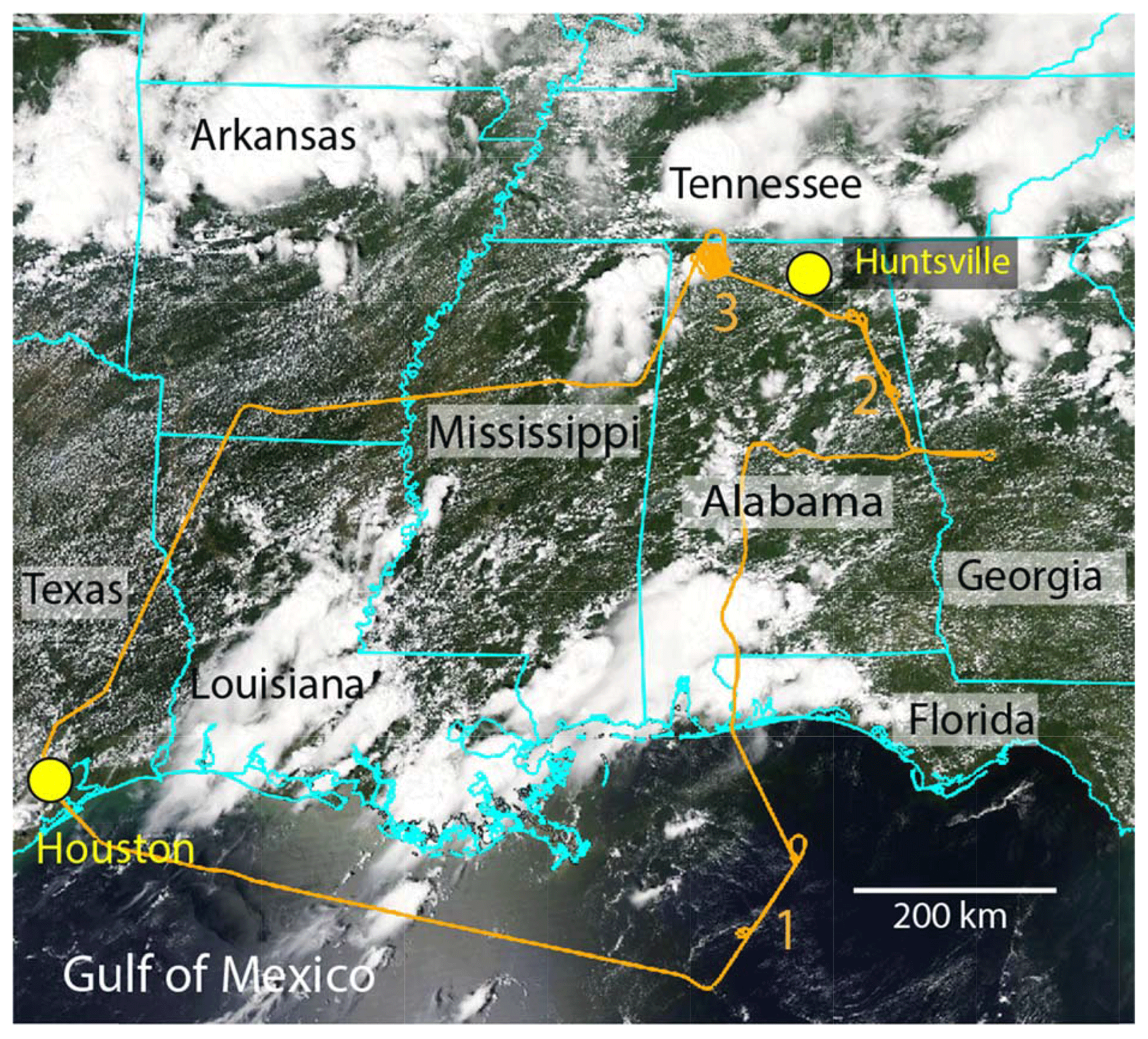
Figure A1 Flight track for the NASA DC-8 (orange) overlaid on the 12 August 2013 Aqua MODIS RGB image. Takeoff and landing were at Houston, Texas. The HSRL site at Huntsville, Alabama, is likewise marked. Coordinated curtain wall profiles with the ER-2 were conducted at labels 1 and 2, followed by the convection spiral discussed at length here at point 3.

To provide context to this analysis, we provide a meteorological overview of the region during the early phases of the SEAC⁴RS study. The period of 5–14 August 2013 was a convectively active period over the SEUS during the summer of 2013. Weak midlevel shortwaves or cold and stationary fronts impinging on high pressure along southern Mississippi, Alabama and Georgia brought convective activity throughout the northern SEUS and Tennessee Valley. While scattered afternoon precipitation formed throughout the region, a stationary front on 11 August over southern Kentucky produced more substantial cells with series of southeastward-propagating outflow boundaries, leading to subsequent convection over northern Alabama and Georgia through the day (Fig. A2). One such band of Cbs passed through Huntsville in the early evening on 11 August. By 12 August, CAPE reached >1800 J kg⁻¹ at sounding sites in the SEUS, leading to scattered Cbs forming in the early morning hours over Tennessee and southeastern Missouri, and propagating into northern Alabama as the day progressed. A significant line of convection reached the northwestern corner of Alabama at 18:00 UTC (where it was sampled by the DC-8 at ∼19:00 UTC), and subsequent convection that formed on the eastward-propagating outflow boundary reached the UAH lidar site 6 h later.

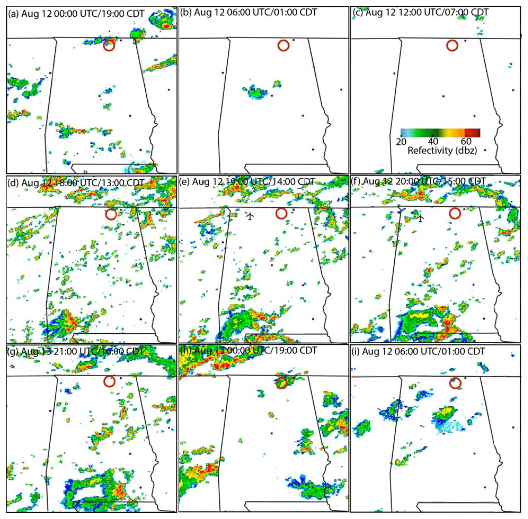
Figure A2 NEXRAD radar reflectivity composites for the 12 August 2013 study case. The red circle indicates the location of the Huntsville HSRL site and black aircraft the location of the DC-8 sampling the cell studied here.

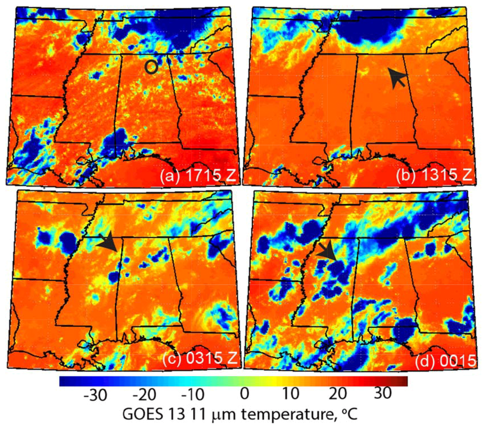
Figure A3 GOES 13 11 µm channel images of the storm leading to AC clouds in the Huntsville lidar data in Fig. 5. (a) PBL detrained AC clouds on 12 August 2013, 17:15 Z; (b) initiation of back trajectory for 0 ^∘C cloud; (c) 10 h back trajectory endpoint to large detrainment shelf; (d) Cb that formed the AC layer.

Regional aerosol loadings for 12 August were consistent with air masses staying within the SEUS over the past several days. AERONET AOD registered a 550 nm AOD of 0.18 at Huntsville in the morning, and Terra MODIS AODs at 550 nm were reported that morning at 0.27 in the vicinity of the Cb sampled. At the surface, regional PM_2.5 stations were reporting daily averaged mass concentrations of 5–10 µg m⁻³ at CSN and SEARCH sites. Specifically at Huntsville, CSN PM_2.5 ranged from 10–14 µg m⁻³ at daybreak and morning hours before dropping to 5–10 µg m⁻³ in the afternoon. Global models (e.g., Session et al., 2015) suggested no significant long-range aerosol transport into the region aside from a pulse of African dust around 8 and 9 August, 3 d before the case day studied here. There was no indication of smoke from the western United States impacting the area. HYSPLIT trajectories spawned at Huntsville were consistent with transport via westerly winds on that day, in an air mass isolated from more pollution in the north. The 2 d back trajectories showed that the middle troposphere air never deviated from northeastern Mississippi and northwestern Alabama. Specific trajectories for Ac layers identified also show origins from storms within this region over 350 km away (Fig. A3). All analyses indicate air masses near the surface through the middle troposphere were regional to the SEUS over the past 2 d, representative of more regional pollution embedded in a regional convective regime.

NEXRAD returns and satellite cloud temperatures (Fig. A3) demonstrate the textural changes in cloud fields as the day progressed from widespread cloudiness to more isolated cells. Above the mixed layer, the sounding was moist but cloud-free, with minor inversions at 3.4 km (perhaps indicating the top of the PBL), 4.6 km (0 ^∘C) and 6.2 km heights. Winds were near constant at 250^∘ above the mixed layer, with steady increases to 12 m s⁻¹ at the 0 ^∘C melting level at 5 km providing only a modest amount of shear (Fig. 3c). Based on the satellite imagery and NEXRAD, the fetch of the air mass over northern Alabama was over mostly Cu to a few isolated but nonprecipitating TCu clouds. The CAPE derived from the UAH sounding was 1650 J kg⁻¹, slightly lower than all of the operational soundings surrounding the site at 12:00 (including Birmingham to the south at 1831 J kg⁻¹ and Nashville to the north at 1811 J kg⁻¹). This neutral state in a convective regime is the midday backdrop against which investigations of clouds in the vicinity of isolated cells is performed in Sect. 4. By late afternoon, the region was more convectively developed, with larger but more scattered individual storms. The one observed by the DC-8 began developing at 19:00 UTC and was monitored until 20:00 UTC. The location of the DC-8 is marked on Fig. A2e and f, although the exact precipitating cell monitored was not observable by NEXRAD until 19:35 when the cloud top height grew to above 6 km. The last NEXRAD return for this cell was at 20:00 UTC.

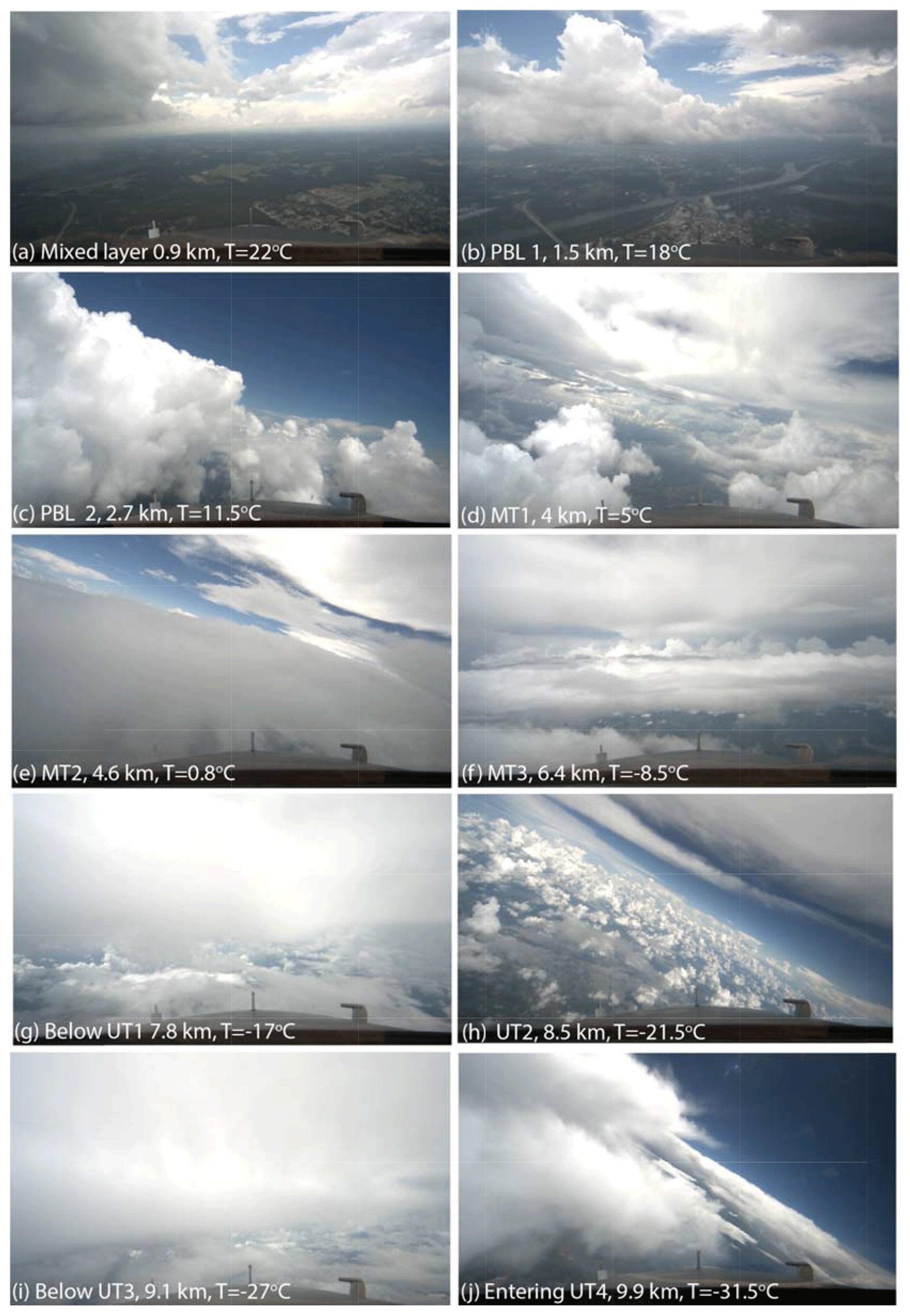
Figure A4 Forward camera images from the DC-8 forward video taken from the leeward spiral along the sampled thunderstorm on 12 August 2014 over northwestern Alabama.

As the day progressed, Cbs repeatedly reformed and then propagated eastward, with one cell in a mature phase reaching the UAH site at 23:00 UTC. This pattern of afternoon thunderstorms persisted for several more days, when large-scale subsidence began to develop behind a weak front that passed through on 14 August.

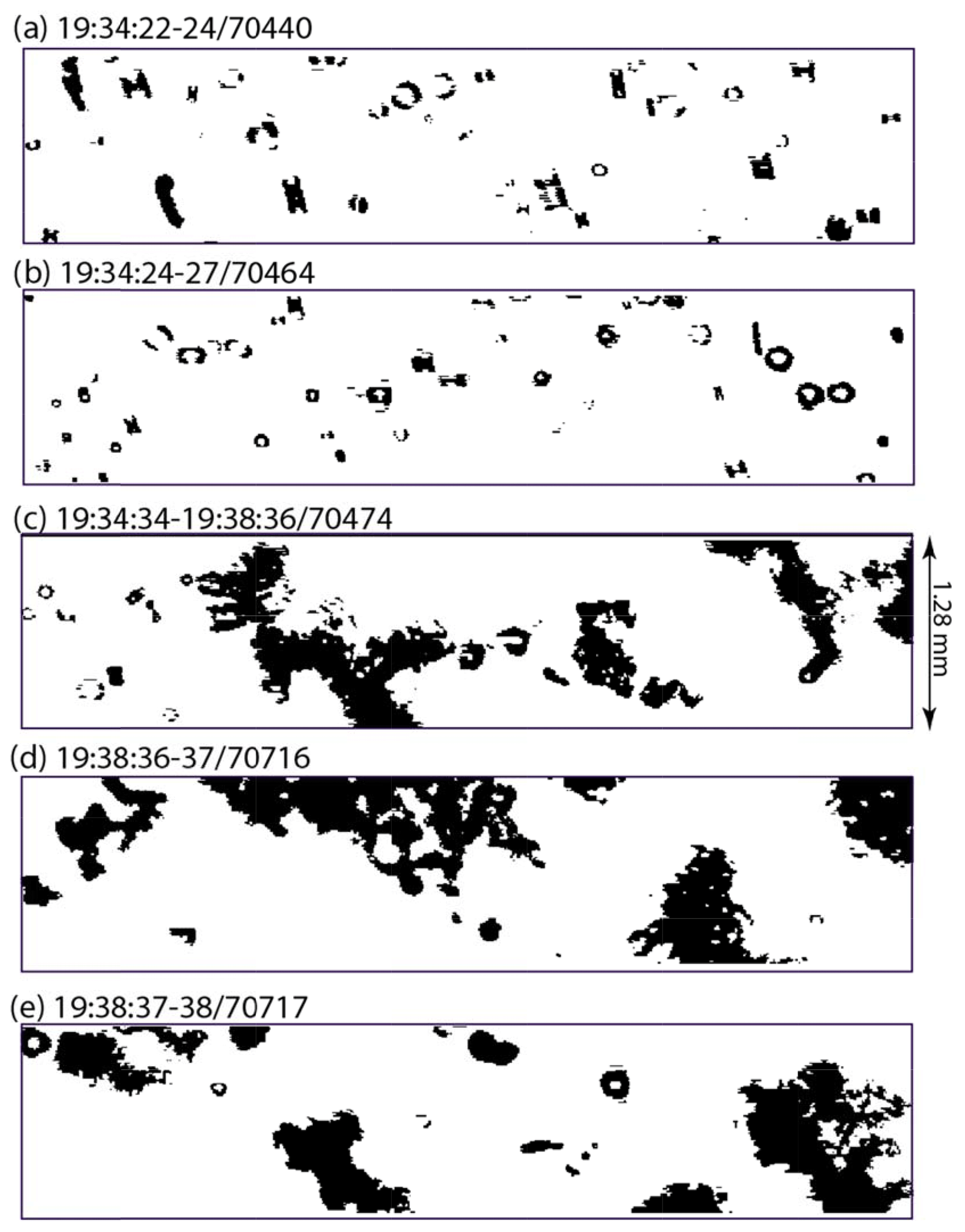
Figure A5 2D-S images of ice for selected periods during layer sampling associated with the right column of Fig. 7. Temperatures were $\sim -\mathrm{10}$ ^∘C, at an altitude of 6.75 km. Annuluses are ice imaged out of focus.

At most levels at temperatures below −9 ^∘C intermittent ice was observed on the SPEC probes (Fig. A5). The SPEC cloud particle probes indicate ice was observed beginning about 19:27 UTC, at temperatures near −9 ^∘C, ranging in size up to around 400–500 µm. Ice is observed on the subsequent climb to colder temperatures at 19:34 UTC (−10 ^∘C), extending to sizes on the order of 1 mm. Intermittent ice, like that observed by the 2-D stereo particle probe and shown in Fig. A5, is observed at subsequently colder temperatures. The 2D-S (Lawson et al., 2006) is a 2-D stereo particle optical array probe that records the cross-sectional image of particles from 10 µm to a few mm in size with 10 µm resolution for determining particle size, concentration, extinction, phase and ice particle habit.