the Creative Commons Attribution 4.0 License.
the Creative Commons Attribution 4.0 License.
 | 04 Jun 2018
Stable sulfur isotope measurements to trace the fate of SO2 in the Athabasca oil sands region
Neda Amiri
Roya Ghahreman
Ofelia Rempillo
Travis W. Tokarek
Charles A. Odame-Ankrah
Hans D. Osthoff
Ann-Lise Norman
Concentrations and δ34S values for SO2 and size-segregated sulfate aerosols were determined for air monitoring station 13 (AMS 13) at Fort MacKay in the Athabasca oil sands region, northeastern Alberta, Canada as part of the Joint Canada-Alberta Implementation Plan for Oil Sands Monitoring (JOSM) campaign from 13 August to 5 September 2013. Sulfate aerosols and SO2 were collected on filters using a high-volume sampler, with 12 or 24 h time intervals.
Sulfur dioxide (SO2) enriched in 34S was exhausted by a chemical ionization mass spectrometer (CIMS) operated at the measurement site and affected isotope samples for a portion of the sampling period. It was realized that this could be a useful tracer and samples collected were divided into two sets. The first set includes periods when the CIMS was not running (CIMS-OFF) and no 34SO2 was emitted. The second set is for periods when the CIMS was running (CIMS-ON) and 34SO2 was expected to affect SO2 and sulfate high-volume filter samples.
δ34S values for sulfate aerosols with diameter D>0.49 µm during CIMS-OFF periods (no tracer 34SO2 present) indicate the sulfur isotope characteristics of secondary sulfate in the region. Such aerosols had δ34S values that were isotopically lighter (down to −5.3 ‰) than what was expected according to potential sulfur sources in the Athabasca oil sands region (+3.9 to +11.5 ‰). Lighter δ34S values for larger aerosol size fractions are contrary to expectations for primary unrefined sulfur from untreated oil sands (+6.4 ‰) mixed with secondary sulfate from SO2 oxidation and accompanied by isotope fractionation in gas phase reactions with OH or the aqueous phase by H2O2 or O3. Furthermore, analysis of 34S enhancements of sulfate and SO2 during CIMS-ON periods indicated rapid oxidation of SO2 from this local source at ground level on the surface of aerosols before reaching the high-volume sampler or on the collected aerosols on the filters in the high-volume sampler. Anti-correlations between δ34S values of dominantly secondary sulfate aerosols with D< 0.49 µm and the concentrations of Fe and Mn (r = −0.80 and r = −0.76, respectively) were observed, suggesting that SO2 was oxidized by a transition metal ion (TMI) catalyzed pathway involving O2 and Fe3+ and/or Mn2+, an oxidation pathway known to favor lighter sulfur isotopes.
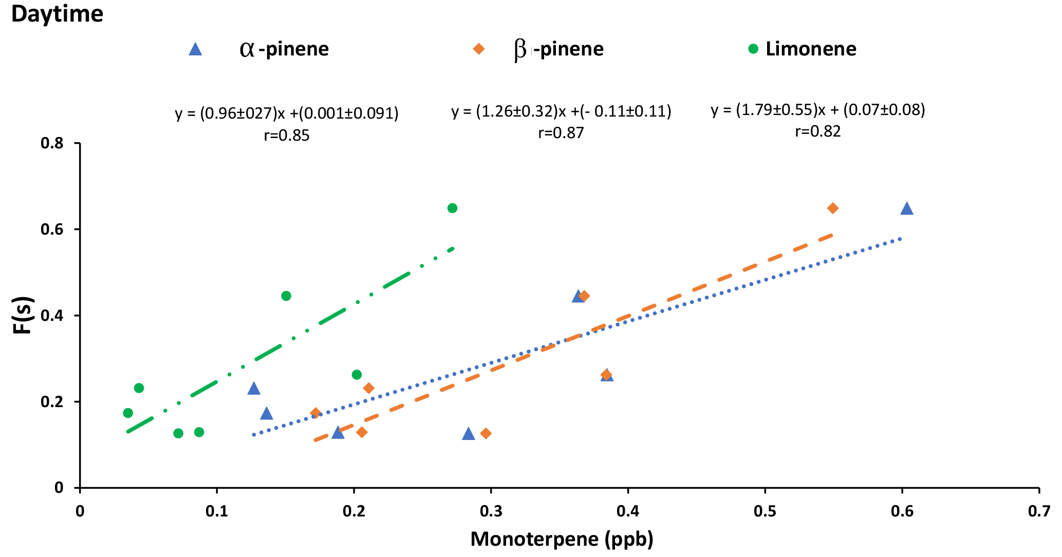
Correlations between SO2 to sulfate conversion ratio (F(s)) and the concentrations of α-pinene (r = 0.85), β-pinene (r = 0.87), and limonene (r = 0.82) during daytime suggests that SO2 oxidation by Criegee biradicals may be a potential oxidation pathway in the study region.
- Article
(8080 KB) - Full-text XML
- BibTeX
- EndNote


Sulfate aerosols are known to impact ecosystems and climate through their deposition and radiative effects. The deposition of sulfate aerosols can cause acidification of soils and lakes (Gerhardsson, 1994). Furthermore, their direct and indirect radiative effects can change the radiative budget at regional scales and alter climate (IPCC, 2001).
Sulfate aerosols can be primary or secondary. Primary particles are emitted directly from the surface to the atmosphere but secondary particles are formed in the atmosphere through gas to particle conversion. The majority of anthropogenic and natural sulfur is emitted as sulfur dioxide (SO2) or oxidized to SO2 in the atmosphere (Berresheim et al., 1995; Berresheim, 2002; Seinfeld and Pandis, 1998). Chin and Jacob (1996) and Chin et al. (2000) estimated that around 50 % of the globally emitted SO2 is oxidized to form sulfate and the remainder is lost by dry and wet deposition.
Dry deposition is important and gives SO2 a lifetime of about 3 days for a boundary layer with 1000 m depth (Hicks, 2006; Myles et al., 2007). Wet deposition is important intermittently for rainy days or days with fog. The lifetime of SO2 in the atmosphere can vary greatly from hours to days depending on measurement location, season, time of day, etc. As an example, Hains (2007) measured SO2 lifetime in the eastern US and found values of 19 ± 7 h. GEOS-Chem simulations suggest a value of 13 h during summer for the same location.
A detailed understanding of SO2 oxidation pathways and their relative importance is critical for accurate representation of sulfate's spatial distribution as well as its impact on climate through aerosol radiative forcing.
The oil sands regions are of great interest because of the large quantities of SO2 emissions (Fioletov et al., 2016; McLinden et al., 2012; Percy, 2013). Therefore, a comprehensive knowledge of SO2 oxidation pathways important in this region is useful to identify where and how atmospheric sulfur species are transported and contribute to aerosol formation, growth, and acid deposition.
Oil sands extraction and upgrading processes can be a source of sulfate aerosols, SO2, and oxidants. The major sources of SO2 emissions in the Athabasca oil sands region are upgrading and energy production operations (Kindzierski and Ranganathan, 2006). Simpson et al. (2010) observed SO2 enhancements over the oil sands region with a maximum value of 39 parts per billion by volume (10−9 ppb) relative to a background value of 102 parts per trillion by volume (10−12 ppt).
Howell et al. (2014) showed that both SO2 and sulfate contributions from the Athabasca oil sands region are significant compared to estimates for potential background sources of sulfur such as annual forest fire emissions in Canada. Bardouki et al. (2003) by the use of positive matrix factorization (PMF) modeling suggested that secondary sulfate is the second most important contributor to PM2.5 mass in Fort MacKay (31 %).
Sulfur dioxide is converted to sulfate in homogeneous and heterogeneous reactions. The oxidation pathway is a very important factor to determine the effects of the sulfate formed on the environment. Gas phase oxidation of SO2 by hydroxyl radicals (OH) produces sulfuric acid (H2SO4) gas, which can nucleate in the atmosphere to form new particles (Tanaka et al., 1994; Kulmala et al., 2004). These newly formed aerosol particles are buoyant and can be dispersed far from the emission source. Newly formed sulfate aerosols also impact direct radiative forcing by scattering sunlight back to space. These particles can grow by the addition of organics to create a large number of accumulation mode aerosols, which are more easily deposited on local surfaces, increasing the potential for acidification at regional to local scales. They also have the ability to form cloud condensation nuclei (CCN; Kulmala et al., 2004, 2007; Benson et al., 2008). After forming CCN they can increase the albedo and lifetime of clouds (Twomey, 1991; Boucher and Lohmann, 1995). Homogeneous oxidation of SO2 in the gas phase by OH is as follows (Burkholder et al., 2015):
A range of 17 to 36 % of global sulfate production can be attributed to this pathway (Chin et al., 2000; Sofen et al., 2011; Berglen, 2004).
Heterogeneous oxidation of SO2 primarily occurs in cloud droplets, although oxidation on the surface of aerosols can be important regionally (Chin and Jacob, 1996). Heterogeneous oxidation prevents H2SO4 gas production and new particle formation. Sulfate formed by this pathway can modify the aerosol size distribution, which affects both direct and indirect aerosol forcing. Scattering efficiency of the particle population can be increased, which is responsible for direct scattering (Hegg et al., 2004; Yuskiewicz et al., 1999). In addition, acidity of aerosols as well as their CCN activity of the particle population can be modified and affect the indirect radiative forcing (Mertes et al., 2005a, b). Eriksen et al. (1972) showed various steps in SO2 dissolution before oxidation by major oxidants, these are H2O2, O3, and O2 catalyzed by transition metal ions (TMIs) such as Fe3+ or Mn2+ in a radical chain reaction pathway (Herrmann et al., 2000).
After the dissolution, S(IV) is oxidized to S(VI) by O3, H2O2, and O2 in the presence of TMIs.
The oxidation of SO2 by O3 and O2 catalyzed by TMIs is pH dependent and becomes faster as pH increases, whereas oxidation by H2O2 within normal atmospheric pH ranges (2–7) does not depend on pH (Seinfeld and Pandis, 1998).
Field studies suggested that TMI-catalyzed oxidation is the dominant sulfate formation pathway in polluted environments in winter (Jacob et al., 1984, 1989; Jacob and Hoffmann, 1983). Oxygen isotope measurements of sulfate aerosols collected at Alert, Canada (82.5∘ N, 62.3∘ W) showed that TMI-catalyzed SO2 oxidation is significant during winter (McCabe et al., 2006). Recent studies have shown that the TMI-catalyzed oxidation pathway is underestimated (more than an order of magnitude) in all current atmospheric chemistry models (Harris et al., 2013a, b). For example, Harris et al. (2013a) measured the sulfur isotopic composition of SO2 upwind and downwind of clouds and used the difference to calculate the fractionation that occurred for in-cloud SO2 oxidation. They showed that SO2 oxidation catalyzed by natural TMIs on mineral dust is the dominant in-cloud oxidation pathway and is underestimated by more than an order of magnitude in current atmospheric models. To the best of our knowledge there is no study to investigate the importance of the TMI-catalyzed pathway in SO2 oxidation on the surface of aerosols in highly polluted areas such as the Alberta oil sands region during summer.
Until recently, OH-radical-initiated oxidation of SO2 was considered the only gas phase oxidation pathway important in the atmosphere. However, recent measurements of the rate constants for oxidation of SO2 by Criegee biradicals and model simulations of field observations have shown this pathway is more significant than previously thought (Berndt et al., 2012; Boy et al., 2013; Mauldin III et al., 2012; Sipilä et al., 2014). Criegee biradicals are formed through ozonolysis of unsaturated hydrocarbons such as biogenic terpenes (Boy et al., 2013; Welz et al., 2012). The rate constants of the reaction of Criegee biradicals and SO2 are somewhat uncertain but researchers agree that the reaction is faster than what has been previously thought (e.g., 6 and 8 cm3 molecule −1 s−1 for Criegee biradicals originating from the ozonolysis of α-pinene and limonene, respectively, Mauldin III et al., 2012). Several studies have linked biogenic volatile organic compound (BVOC) environments to an increase in SO2 to sulfuric acid and/or sulfate conversion rates. For example, Mauldin III et al. (2012) reported the oxidation of SO2 by Criegee biradicals faster than what has been thought before, during a field study in a boreal forest and confirmed the results by laboratory and theoretical studies.
In this study, we investigated the importance of the various SO2 oxidation pathways, including Criegee biradicals in a polluted region with high volatile organic compound (VOC) emissions using measurements of sulfates, SO2 concentrations, and isotopic composition.
Sulfur isotope analysis is a powerful tool to investigate SO2 oxidation pathways in the atmosphere. As an example, Lin et al. (2017) used high-sensitivity measurements of cosmogenic 35S in SO2 and sulfate from the ambient boundary layer over coastal California and the Tibetan Plateau to identify oxidation of SO2 to sulfate. The lifetime in summer ranged from 1 to 2 days suggesting that there might be oxidation pathways which are more important than previously thought.
In this study, stable sulfur isotope values for SO2 and size-segregated sulfate aerosols were measured. δ34S values of potential sources in the region (Proemse et al., 2012a) and isotope fractionation data (Harris et al., 2012) were used to investigate atmospheric sulfur oxidation pathways in the Athabasca oil sands region. The sulfur dioxide to sulfate conversion ratio was also used as a tool to investigate the possible SO2 oxidants in the region. Although the data represent a short period of time and do not reflect the variability on a seasonal timescale, Soares et al. (2018) showed that short-term measurements are more suitable for source identification. They mentioned that the source signals of NO2 and SO2 emissions are available in hourly to daily timescales and long-term observation may cause a loss in short term variation.
Sulfate aerosols and SO2 measurements were made at a monitoring site next to the Wood Buffalo Environmental Association's (WBEA) air monitoring station 13 (AMS 13) site just south of Fort MacKay in the Athabasca oil sands region from 13 August to 5 September 2013 as part of the Joint Canada-Alberta Implementation Plan for Oil Sands Monitoring (JOSM) project (Liggio et al., 2016; Phillips-Smith et al., 2017). The location of AMS 13 is shown in Fig. 1.
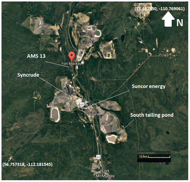
Figure 1The Wood Buffalo Air Monitoring Station 13 (AMS 13) site, south of Fort MacKay (map data© 2018 Google)
Stable sulfur isotopes can be used to investigate sulfur sources, transport, and chemistry such as the relative importance of oxidation pathways (Puig et al., 2008; Krouse and Grinenko, 1991). Sulfur has four stable isotopes: 32S, 33S, 34S, and 36S with relative abundances of ∼ 95, 0.75, 4.21 and 0.015 %, respectively. The isotopic composition is described using the delta notation:
where n is the number of atoms, xS is the heavy isotope and V-CDT is the international sulfur isotope standard, Vienna Canyon Diablo Troilite, with the isotopic ratio of , (Ding et al., 2001) and . For the purpose of this paper we only analyze δ34S values and use δ33S values to find enrichment of samples.
The isotopic composition (δ34S) of major sources of atmospheric sulfur in the Athabasca oil sands region were quantified by Proemse et al. (2012a). They reported sulfur isotope values for bitumen, (+4.3 ± 0.3 ‰), untreated oil sands, (+6.4 ± 0.5 ‰), and the isotopic composition of products such as (NH4)2SO4, which is produced in flue-gas desulfurization, (+7.2 ‰), coke (+4.0 ± 0.2 ‰), and elemental sulfur (+5.3 ± 0.5 ‰). Primary sulfate with diameter D< 2.5 µm are reported to have δ34S values between +7.0 ‰ and +7.8 ‰ with an average of +7.3 ± 0.3 ‰, and between +6.1 ‰ and +11.5 ‰ with an average of +9.4 ± 2 ‰ for two of the largest stacks in the region. These two stacks are 12.2 and 19.4 km south and southeast of the measuring site, respectively.
In addition to sulfur emissions from oil sands processing, aerosols can potentially be produced from vehicle exhaust. Combustion emissions from vehicles showed a δ34S of +5 ‰ for SO2 from engine exhaust in Alberta and British Columbia (Norman et al., 2004; Norman, 2004). On average, diesel and gasoline contained very low amounts of sulfur (0.008 %, Norman, 2004) and combustion produces both primary sulfate as well as SO2. Other sulfur emissions in the region may result from anoxic conditions in the environment or the tailing ponds associated with sulfate-reducing bacteria. Biogenic emissions of hydrogen sulfide (H2S) have negative δ34S values which can be as negative as −30 ‰ (Wadleigh and Blake, 1999). H2S is oxidized to SO2 with a lifetime of 1 day (Brimblecombe et al., 1989) and the sulfur isotopic composition is not expected to change during oxidation of H2S to SO2 (Sanusi et al., 2006; Newman et al., 1991).
Differing isotopic contributions from sulfur sources can drive variations in aerosol sulfate δ34S values. Another reason for δ34S variation can be isotopic fractionation. The oxidation of SO2 causes isotope fractionation between the products and reactants as long as the reaction is not complete. When the reactant is available as an infinite reservoir, the fractionation factor is calculated as
where . Following the definition for α used by Harris et al. (2012) for both kinetic and equilibrium reactions, α<1 means that the light isotopes react faster, so products are isotopically lighter than the reactant.
During this study, minute quantities of 34SO2 were emitted from a chemical ionization mass spectrometer (CIMS) exhaust 50 m away from the high-volume sampler near the ground for special periods. Here we refer to these particular periods as CIMS-ON. The enrichment of 34SO2 was sufficiently large that isotopic fractionation can be neglected during CIMS-ON periods. However, sulfur sources and oxidation pathways can be examined using δ34S values for the periods when CIMS was not operational (CIMS-OFF). During SO2 oxidation to sulfate, isotope fractionation occurs between reactants and products which is unique for each oxidation pathway. Note that sulfur isotope fractionation resulting from oxidation by Criegee biradicals is not currently known. Harris et al. (2012) reported temperature dependent fractionation factors for different SO2 oxidation pathways as follows: SO2 oxidation by OH radicals favors heavy isotopes and the fractionation decreases slightly with temperature (Eq. 3).
Aqueous phase oxidation can occur by H2O2 and O3, and fractionation during this pathway (Eq. 4) also prefers heavy isotopes and decreases with temperature slightly.
The fractionation during the TMI-catalyzed oxidation pathway acts in the opposite direction to the other two pathways. TMI-catalysis is the only known oxidation pathway which favors lighter isotopes in the product sulfate and the fractionation strongly depends on temperature (Eq. 5).
4.1 Field measurements
Temperature, relative humidity, and wind speed and direction time series are shown in Fig. A1 in the Appendix. A diurnal cycle in relative humidity (RH) is evident for all days during the campaign except 25 August which was a rainy period.
A high-volume sampler placed at ground level with a flow rate of 0.99 ± 0.05 m3 min−1 was used to collect aerosols and SO2. The high-volume sampler was fitted with a five-stage cascade impactor to collect size-segregated aerosols on glass fiber filters in five ranges of aerodynamic diameter as A (>7.2 µm), B (3.0–7.2 µm), C (1.5–3.0 µm), D (0.95–1.5 µm), and E (0.49–0.95 µm). The final filter for fraction F< 0.49 µm was a 20.3 cm × 25.4 cm glass filter to collect aerosols with D<0.49 µm. An SO2 filter pretreated with potassium carbonate (K2CO3) and glycerol solution was located beneath these six size-segregated aerosol filters (Norman, 2004). The sampling interval was 12 h (daytime 05:00 to 17:00 MDT (Mountain Daylight Time) and nighttime 17:00 to 05:00 the next day) for the first 12 days except 20 and 27 August after which samples were collected for 24 h (05:00 to 05:00). Field blanks were collected on three separate occasions at the start, in the middle, and at the end of the campaign. Filter blanks from the field were loaded and then unloaded, stored, and analyzed using the same protocols as samples. The high-volume sampler was turned off during field blank sampling. Filters were stored in ziplock bags and kept at temperatures less than 4 ∘C and transferred to the lab for analysis.
WBEA SO2 data were used with a sampling interval of 5 min. Ozone and NO2 mixing ratios were measured by UV absorption using a Thermo 49i O3 monitor every 10 s and a blue diode laser cavity ring-down spectrometer every 1 s, respectively (data were averaged to 1 min; Odame-Ankrah, 2015; Paul and Osthoff, 2010). The slope uncertainties in these measurements were ±1 and ±10 %, respectively. Radiometer measurements using a pair of spectral radiometers (one facing the zenith, the other the nadir direction) were used to determine actinic flux and to calculate photolysis frequencies (j values; Osthoff et al., 2018). Iron (Fe) and Manganese (Mn) were measured by semi-continuous X-ray fluorescence measurements of metals taken every hour on a filter tape with a measurement uncertainty of ±10 % (Phillips-Smith et al., 2017).
Monoterpenes were measured hourly by gas chromatography ion-trap mass spectrometry (GC-IT-MS; Tokarek et al., 2017). VOCs and C2-C12 were sampled in canisters over a period spanning 09:30 to 08:30 of the next day, and analyzed using gas chromatography mass spectrometery (GCMS). Detection limits for VOC measurements can be found in the online JOSM database (ftp://arqpftp:research@ftp.tor.ec.gc.ca/OS/AMS13, last access: 10 October 2017).
A chemical ionization mass spectrometer (CIMS) similar to the one described by Sjostedt et al. (2007) was used to measure OH reactivity at a distance of 10 m horizontally from the high-volume sampler. Enriched 34SO2 was emitted from an exhaust pipe at ground level less than 50 m to the east in an unused area containing shrubs. Enriched 34SO2 affected a portion of our samples during CIMS-ON periods; these periods were used to trace the fate of local 34SO2 emitted from the CIMS exhaust near the ground.
4.2 Analysis of high-volume filter samples
Filter papers were shredded and sonicated for 30 min in distilled deionized water in the laboratory (200 mL for SO2 filters and filters to collect particles in the size range F< 0.49 µm and 75 mL for slotted filters to collect particles in sizes larger than 0.49 µm). For SO2 filters, 1 mL of 30 % w/w hydrogen peroxide (from BDH) was added to oxidize the SO2 to sulfate before sonication. Filter paper fibers were removed by 0.45 mm Millipore filtration, and 10 mL of the filtrate samples was analyzed using a Dionex ICS-1000 ion chromatography (IC) system with a Dionex IonPac AS14 column and electric conductivity detector to determine the concentration of sulfate with an uncertainty of 5 %. Prior to treatment, the pH of the remaining filtrate was measured and found to be ∼ 6.0. The remaining filtrate was treated with 0.5 mL of 10 % BaCl2 (dihydrate 99 %, from EMD), and dilute (0.5 normal) OmniTrace HCl (34–37 %, from EMD) was added to samples until a pH of 3 was achieved. Approximately 100 µL of 0.5 normal HCl was used for aerosol filters. The samples were then heated to facilitate precipitation of BaSO4. Barium sulfate was isolated by Millipore filtration, and dried samples were packed into tin cups and analyzed with a PRISM II continuous-flow isotope ratio mass spectrometer (CF-IRMS) to obtain δ34S values (relative to V-CDT; Giesemann et al., 1994). The precision in measuring δ34S is ±0.3 ‰ which is determined as the standard deviation (1σ) of δ34S for several standard runs. δ34S measurements were blank corrected using the sulfur concentration and δ34S values for field blanks. Insufficient sulfate was present for some samples after concentration blank correction. Although the concentration of sulfate was too small to perform blank correction for some samples, they displayed the same range for δ34S values as those which were blank corrected. This suggests little to no bias was introduced by blank correction. Therefore, δ34S values are reported from some samples which were not isotopically blank corrected. These samples are indicated with a * in Tables 1 and 2.
The PRISM II continuous flow isotope ratio mass spectrometer measures δ34S and δ33S simultaneously and the values for non-enriched samples were expected to be related according to the mass dependent fractionation (MDF) relation (δ33S∼0.51δ34S). For this experiment, some of the samples were enriched in 34S and they were identified by the use of the MDF relation between δ34S and δ33S of the standards for the same run. δ33S∕δ34S was averaged for standards for each run and was used as a cutoff criterion and data falling below this criterion were tagged as enriched.
Care was taken to analyze sufficient standards and blanks between enriched samples (CIMS-ON periods) to ensure carryover was minimal. Little to no deviation in standards and blanks was apparent after enriched δ34S values from CIMS-ON periods were analyzed. In this paper uncertainties are reported as 1σ standard deviation.
4.3 Natural tracer experiment
4.3.1 Sulfur 34S release
The CIMS was operated between 12 August 12:00 to 14 August 12:00 and 20 August 12:00 to 7 September 09:45 MDT. Ten standard cubic centimeters of 0.9 % 34SO2 was diluted in 30 SLPM N2 to obtain a mixing ratio of 3 ppm for 34SO2 in the sample flow. 34SO2 reacts with OH to form which is ionized by to form and ions that are detected at 99 and 49 in the negative ion spectrum of the mass spectrometer. An excess amount of 34SO2 compared to the required 34SO2 to complete titration of OH in the sample flow was used for ambient air OH reactivity measurements. Almost all of the flow entering was exhausted by the instrument which contained excess 34SO2 and formed . In 1 min, . Some of the formed is also lost by wall loss in the instrument so the majority of the exhaust is in the form of 34SO2. For the periods when the CIMS was operational (CIMS-ON), significant 34S isotope enrichment was observed; therefore, samples were divided into two sets, CIMS-ON and CIMS-OFF.
The first set is for samples collected during the shutdown periods of the CIMS (CIMS-OFF). These CIMS-OFF periods were used to investigate the isotopic composition of size-segregated sulfate aerosols and SO2 in the region and the possible sources and formation pathways of sulfate aerosols. The second set (CIMS-ON) is for samples affected by enriched 34S and is not used as an indicator of sulfur isotopic composition of sulfate aerosols in the region. Instead, the enriched 34SO2 is used as a natural tracer to follow the fate of SO2 emitted from a local ground-based source and its oxidation.
4.3.2 Sulfur conversion ratio
In this paper we use the sulfur conversion ratio, which is defined as the portion of SO2 which is converted to particulate sulfate:
In this formula, [SO4] is the concentration of sulfate aerosols with D< 0.49 µm. In this study the sulfate is dominantly secondary (Proemse et al., 2012a), corroborated here by the absence of soil indicators (Sect. 5.1). F(s) can be affected by dry deposition. Since little is known about the appropriate dry deposition velocities in this region, potential variations between SO2 and sulfate dry deposition rates are neglected in the analysis.
Since F(s) is a measure of SO2 to sulfate conversion, it is a measure of oxidant loading. Therefore, significant positive correlation between F(s) and other compounds may be an indicator of the importance of that compound as a tracer for SO2 oxidation. This formula can be used for both CIMS-ON and CIMS-OFF periods since the number of enriched molecules reaching the high-volume sampler is very small and cannot change F(s). The number of enriched molecules reaching the high volume sampler is calculated using equations described in Sect. 4.3.3 and the fraction of enriched molecules in comparison to the total sulfur concentration is reported in Table A1.
4.3.3 Concentration of 34S enriched molecules
The concentration of enriched molecules as 34SO2 and 34SO4 were calculated using the following equations during CIMS-ON periods. Isotope ratio (R) values show the ratio of sulfur isotopes to the most abundant isotope, which is 32S for sulfur.
in which n34S* is the number of 34S atoms reaching the filter from the CIMS exhaust and Stotal is the total number of sulfur atoms on the filter. The R34 value is calculated as the average of R34 values for samples without enrichment. There were R33 data available from the IRMS but the uncertainty was high (±3 ‰) and we used the value for the international standard for sulfur V-CDT. 36S is included in calculations since the amount of 34S* from the CIMS exhaust is on the same order of magnitude. values were available for each sample. The concentration of sulfate for each sample was available from IC and the number of sulfur atoms as SO2 or sulfate can be calculated. Then the number of 34S from CIMS was calculated and divided by the volume of total sampled air and the number of and molecules cm−3 was calculated (Table A1).
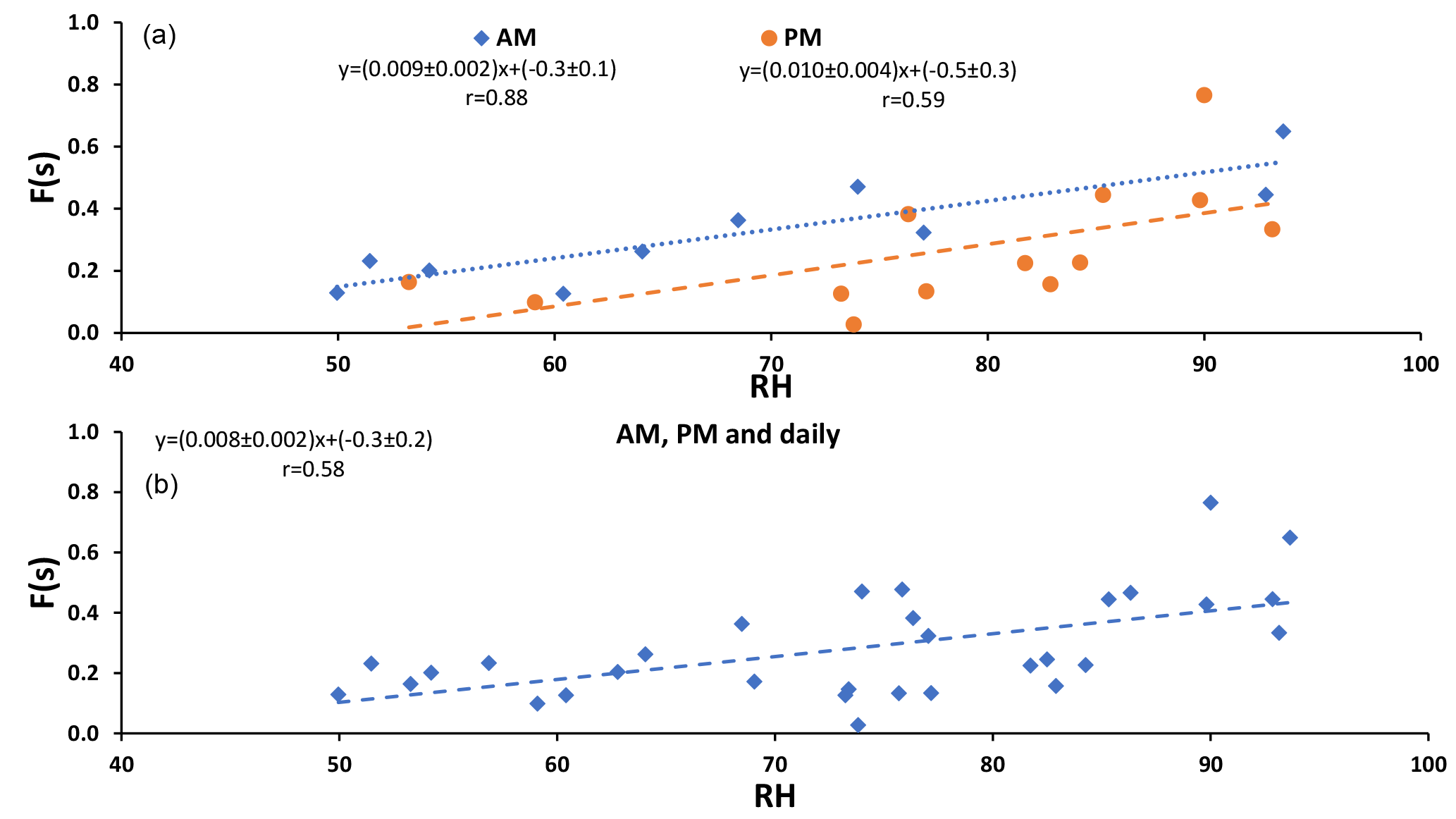
Figure 2F(s) (CIMS-ON and CIMS-OFF) versus relative humidity (RH). (a) correlation during daytime (AM) and nighttime (PM) and (b) correlation for daytime, nighttime, and daily data. P value < 0.05.
5.1 Sulfur conversion ratio (F(s))
The sulfur conversion ratio (F(s), Eq. 6) was calculated for the smallest size fraction of measured sulfate (F< 0.49 µm). Absence of Ca and Mg in this size fraction (all concentrations were below the IC detection limit of 0.1 mg L−1) indicates that primary soil particles were not present in this size fraction. Proemse et al. (2012a) suggested that less than 10 % of total sulfur emissions from two major stacks in the region in PM2.5 were primary sulfate. Therefore, primary sulfate from stacks do not form a significant portion of sulfate aerosols in the D< 0.49 µm size range. Based on these two pieces of information, it is expected that sulfate particles on this size fraction are mostly (> 90 %) secondary. As a result, F(s) gives valuable information about which pathways dominate SO2 oxidation and formation of sulfate aerosols.
F(s) is not affected by enriched sulfate emissions during CIMS-ON periods (because the amount of 34SO2 emitted was relatively small, Table A1). Hence, F(s) reflects the conversion of SO2 to sulfate for the entire measuring period. This implies negligible changes to F(s) values because of the CIMS emissions.
F(s) (CIMS-ON and CIMS-OFF) is plotted versus relative humidity in Fig. 2. Positive correlations were observed for daytime (AM) and nighttime (PM) and daily samples (r = 0.88, r = 0.59, r = 0.58, respectively) with the same slope (≃ 0.01).
F(s) values were usually higher during the daytime in comparison to nighttime values (Tables 1 and 2), which was what we expected for OH-driven oxidation during daylight. In the troposphere, the OH radical is produced mainly from photolysis of O3 to O(1D) and subsequent reaction with water vapor. If a steady state in O(1D) is assumed with respect to its production and loss, the (instantaneous) daytime OH production rate is proportional to . A negative correlation was observed between F(s) and this (integrated) OH production rate during the daytime (r = −0.72, P value < 0.05; Fig. A2). However, two data points with the highest RH (25 and 26 August) drive this correlation, and no correlation was observed for the remainder of the samples. This suggests that there may be SO2 oxidation pathways in addition to OH during the day in this region.
The time series for SO2 during the campaign is shown in Fig. 3a. The time series was dominated by spikes in the SO2 mixing ratio. Phillips-Smith et al. (2017) used PMF to determine concentration time series for five factors during the campaign. This analysis showed that on the 14, 23, and 24 August and 3 and 4 September were periods that the site was impacted by upgrader emissions. Concentrations of SO2, Fe, and Mn (measured in PM2.5) were markedly higher during these periods (Fig. 3).
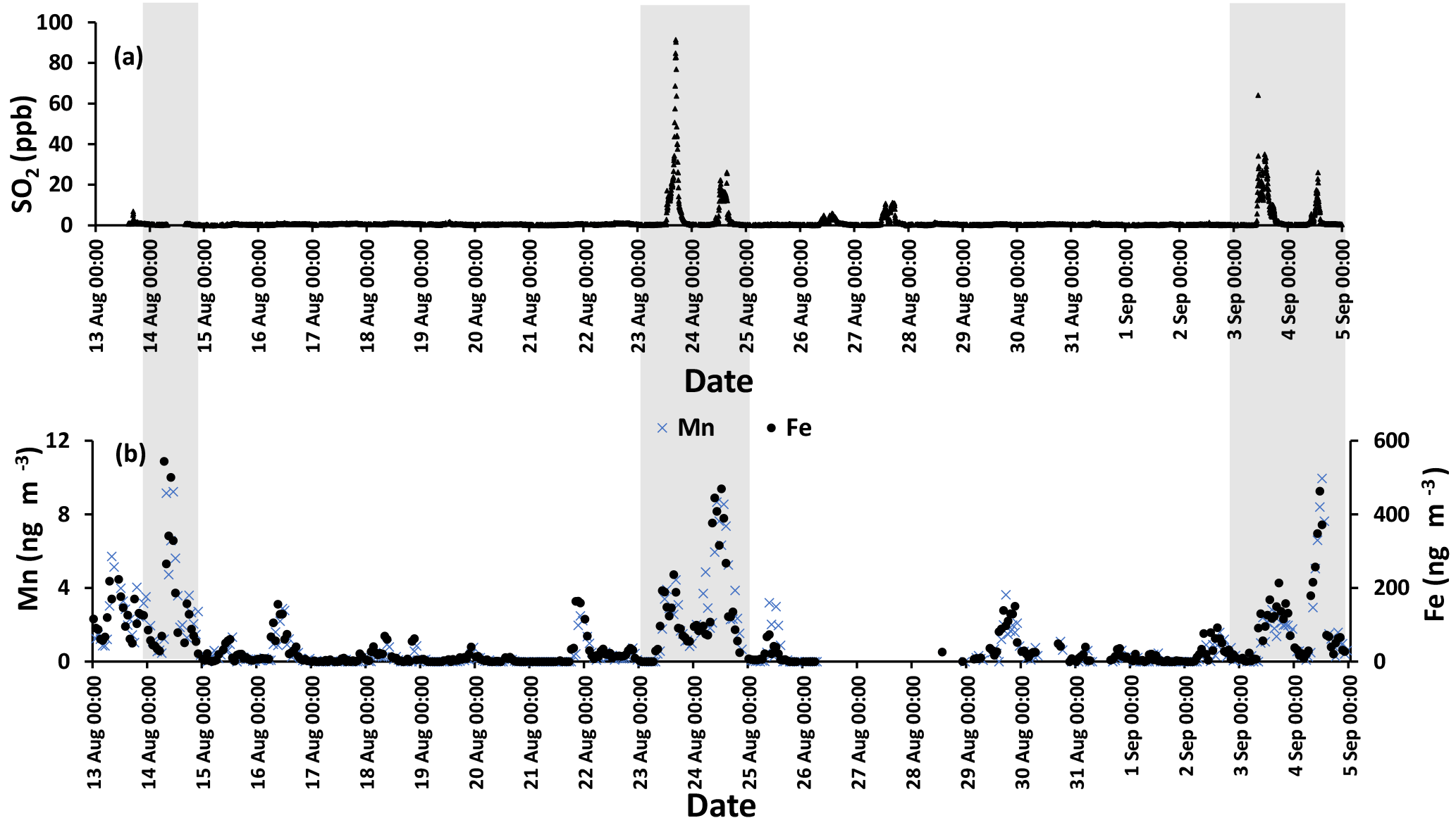
Figure 3(a) SO2 time series with a sampling interval of 5 min (there is a gap in 14 August data) and (b) hourly data for Mn (left axis) and Fe (right axis). Shaded areas indicate polluted periods.
It is interesting to note that F(s) for daytime was higher than nighttime for all samples except periods when the site was impacted by plumes from major oil sands upgrading facilities (polluted periods; Phillips-Smith et al., 2017). A comparison between AM and PM values for F(s) for 23 and 24 August showed that nighttime values were almost double the daytime values. F(s) data were not available for the daytime of 14 August to compare with the nighttime value, but 14 August PM showed the highest value for F(s) (0.77) during the entire campaign (Tables 1 and 2). At night, aqueous phase oxidation is believed to be the dominant SO2 transformation pathway as OH is absent (Chin and Jacob, 1996). No correlation was observed between the F(s) and O3 mixing ratio for daytime, nighttime, or daily samples (Fig. A2). Therefore, it is expected that SO2 oxidation occurs by the H2O2 and/or the TMI-catalyzed pathways.
Fe and Mn concentrations in PM2.5 aerosols, averaged over the nighttime high-volume sampling periods, are shown in Fig. A3 (Phillips-Smith et al., 2017). The averaged nighttime concentrations of Fe and Mn were higher during polluted periods (average values of 57 ± 20 ng m−3 and 1.5 ± 0.5 ng m−3, respectively) in comparison to other periods (average values of 9 ± 3 ng m−3 and 0.13 ± 0.06 ng m−3, respectively; Fig. A3). The data collected on 21 August PM were excluded from this analysis because the PMF analysis by Phillips-Smith et al. (2017) showed this period to be distinct (discussed further below). To check if the TMI-catalyzed pathway played a role in SO2 oxidation during nighttime, averaged concentrations of Fe and Mn were added and [Fe + Mn] × [H2O] values were calculated and shown in Fig. 4a. F(s) is also shown for nighttime samples (Fig. 4b). When [Fe + Mn] × [H2O] values are high, F(s) is also high.
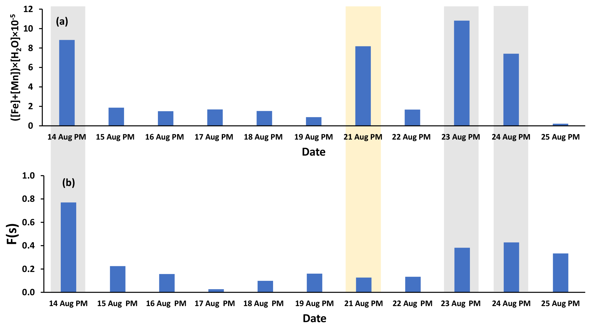
Figure 4(a) ([Fe] + [Mn]) × [H2O] values for nighttime (PM) samples as an indicator of the TMI-catalyzed SO2 oxidation pathway (Fe and Mn concentrations were averaged over the running periods of the high-volume sampler) and (b) F(s) values for the nighttime samples. Polluted periods and the soil episode are shown by gray and yellow shaded areas, respectively.
Concentrations of Fe and Mn were associated with upgrader, soil, and haul road dust factors during polluted nighttime periods (14, 23, 24 August: Phillips-Smith et al., 2017). Although 21 August PM was not a polluted period, it showed high [Fe + Mn] × [H2O] values but F(s) was not high (Fig. 4b). For 21 August, the analysis by Phillips-Smith et al. (2017) showed that there was a peak for the soil factor but not upgrader and haul road dust. F(s) on this night was markedly lower than during periods when upgrader and haul road dust factors were high. F(s) for 25 August was also high since this was a rainy period (Sect. 4.1).
5.2 δ34S values for size-segregated sulfate aerosols and SO2 during CIMS-OFF periods
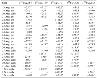
During CIMS-OFF periods 34SO2 emissions were absent, so δ34S values reflect the sulfur isotopic composition of the sulfur compounds in the region and/or fractionation as the SO2 is oxidized and transported to the AMS 13 site. δ34S values during CIMS-OFF periods for SO2 and size-segregated sulfate in size ranges F< 0.49 µm , E0.49−0.95 µm, D0.95−1.5 µm, C1.5−3.0µm, B3.0−7.2 µm, and A> 7.2 µm are shown in Table 1. Possible oxidation pathways of SO2 to sulfate were investigated using these δ34S values.
Blank corrected δ34S values for SO2 were +5.1 and +10.8 ‰. No negative δ34S values were observed for SO2. If it is assumed that no fractionation occurred during formation of primary sulfate in major stacks, then it is expected that δ34S values for SO2 would be the same as primary sulfate (with an average of +7.3 ± 0.3 ‰ and +9.4 ± 2.0 ‰). The δ34S values of SO2 ranged from +5.1 to +11.1 ‰ (Table 1) and are consistent with this assumption. The lowest value (+5.1 ‰) is consistent with a δ34S value for SO2 from vehicle exhaust (Table 1).
δ34S values for size F< 0.49 µm particles ranged between +1.8 and +15.1 ‰ with an average of +7.4 ± 4.2 ‰. Although this average overlaps with values given by Proemse et al. (2012b) for primary sulfate from the stack emissions (+7.3 ± 0.3 and +9.4 ± 2.0 ‰), there were δ34S values lighter and heavier than what was expected from potential sulfur sources in the region in this size range. Therefore, δ34S of sulfate cannot be used as a quantitative indicator for industrial SO2 emissions as isotope fractionation may have occurred as the stack emissions (SO2) were transported to the AMS 13 site. As shown in Sect. 5.1 sulfate particles in this size range are predominantly secondary; therefore, these data can be used to investigate the importance of different SO2 oxidation pathways during transport.
Table 1δ34S (‰) values for SO2, and sulfate aerosols in size ranges F< 0.49 µm, E0.49−0.95 µm, D0.95−1.5 µm, C1.5−3.0 µm, B3.0−7.2 µm, and A> 7.2 µm during CIMS-OFF periods. Not blank corrected samples have an uncertainty of ± 0.3 ‰, and the uncertainty for blank corrected samples are shown in parentheses.
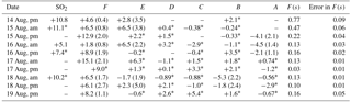
* not blank corrected samples.
Particles in larger size ranges (E0.49−0.95 µm, D0.95−1.5 µm, C1.5−3.0 µm, B3.0−7.2 µm, and A> 7.2 µm) are expected to contain more primary sulfate and have lower δ34S values in comparison to the F< 0.49 µm size range. There were no negative values for sulfate particles in the size fraction F< 0.49 µm, but negative values were observed for the size fraction E0.49−0.95 µm. There was a tendency to lighter δ34S values for larger sulfate particles as shown in Fig. 5.
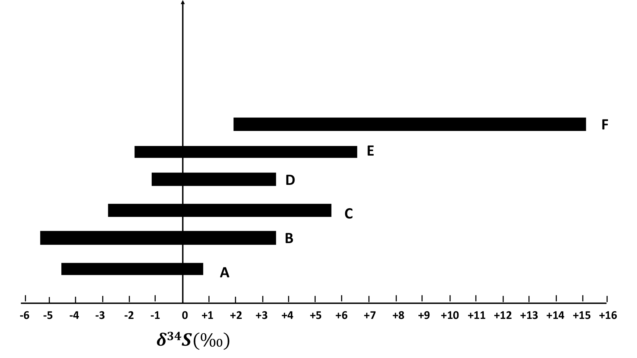
Figure 5δ34S ranges for F< 0.49 µm, E0.49−0.95 µm, D0.95−1.5 µm, C1.5−3.0 µm, B3.0−7.2 µm, and A> 7.2 µm size ranges during CIMS-OFF periods. As the particles become larger, δ34S becomes more negative.
5.2.1 Correlation between Fe and Mn and sulfate concentration and δ34S values during CIMS-OFF periods
Sulfur dioxide can be oxidized in the aqueous phase by O2 in the presence of TMIs predominantly by Fe3+ and Mn2+(Herrmann et al., 2000). If this is an important oxidation pathway, more secondary sulfate is expected to be produced when the concentrations of catalysts are higher. Since concentrations of Fe and Mn were measured in PM2.5 particles, the concentration of sulfate in impactor size fractions (F< 0.49 µm, E0.49−0.95 µm, D0.95−1.5 µm, and C1.5−3.0 µm) were added to find the concentration of sulfate in particles with D< 3 µm. The sulfate concentration in the impactor size range D< 3 µm is almost the same as the concentration in PM2.5 since the concentration in size fraction C1.5−3.0 µm was very low (zero for all periods except polluted periods, which ranged between 0.58 and 1.76 µg m−3). The concentration for particles from the impactor with D< 3 µm is plotted versus Fe and Mn concentrations and the sum of Fe and Mn in Fig. 6. Positive correlations were observed for all three cases (r = 0.86, r = 0.89, r = 0.86, respectively; Fig. 6). Positive correlations were also observed when the concentrations of sulfate in the aerosol size fractions F< 0.49 µm and E0.49−0.95 µm were plotted against the concentrations of Fe and Mn and the sum of Fe and Mn (Fig. A4). There were not enough sulfate concentration data for size fractions C1.5−3.0 µm and D0.95−1.5 µm to show the individual correlations with Fe, Mn, and the sum of Fe and Mn.

Figure 6Sum of concentrations of sulfate in size ranges F< 0.49 µm, E0.49−0.95 µm, D0.95−1.5 µm, and C1.5−3.0 µm versus the concentration of (a) Fe, (b) Mn, and (c) Fe + Mn.
When SO2 is oxidized by the TMI-catalyzed pathway, the sulfur isotopic composition of the sulfate formed is lighter than the isotopic composition of the reactant SO2 (Harris et al., 2012). Significant anti-correlations were apparent for sulfate δ34S values in the size fraction F< 0.49 µm when plotted against Fe and Mn concentrations (r = −0.80 and r = −0.76, respectively; Fig. 7). This suggests that lighter δ34S values occur in secondary sulfate in the presence of higher concentrations of Fe and Mn. Insufficient isotope data were available to create similar plots for other size fractions.
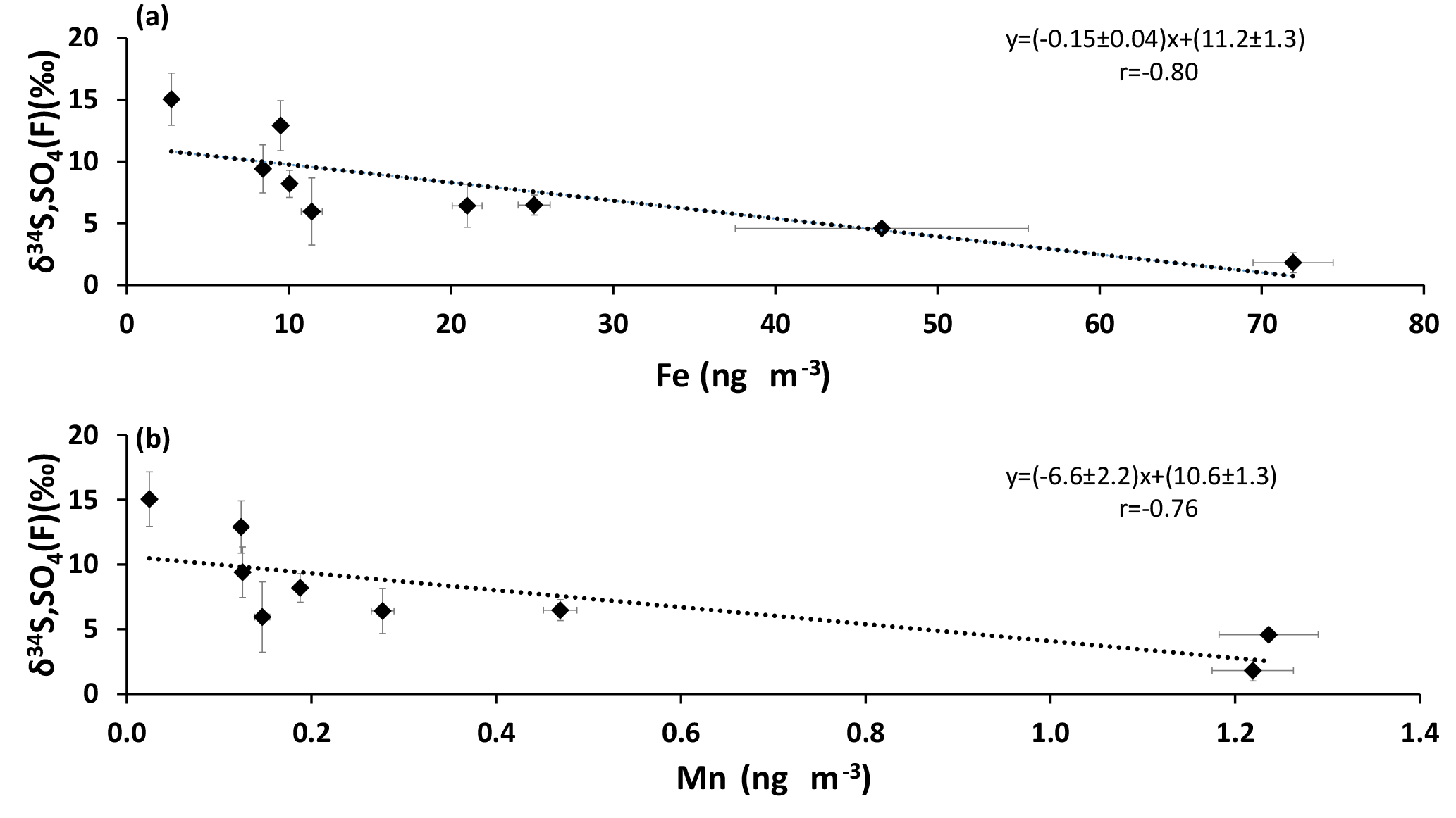
Figure 7δ34S values of size FD< 0.49 µm sulfate aerosols versus the concentrations of (a) Fe and (b) Mn.
Positive correlations were also observed between concentrations of Fe and Mn and the concentration of SO2 (r = 0.67 and r = 0.65, respectively; Fig. A5), which may indicate that they originate from the same source, or were transported together to the sampling site.
5.3 δ34S values of SO2 and size-segregated sulfate aerosols during CIMS-ON periods
The release of 34SO2 from the CIMS allowed for an examination of SO2 oxidation to sulfate under field conditions. An unexpected result was found: δ34S values for SO2 and sulfate samples with D< 0.49 µm during the periods when the CIMS was operated (CIMS-ON) are shown in Table 2. The blank corrected data show that δ34S values for enriched SO2 samples were only as high as +35.6 ‰, and there were values without enrichment ranging between +4.8 and +10.9 ‰ with an average value of +8.3 ± 1.8 ‰. All sulfate samples in the size range F< 0.49 µm representing SO2 oxidation during the CIMS-ON periods were blank corrected, and all AM and PM samples were highly enriched in 34S; the δ34S values were as high as +913 ‰ (Table 2).
A comparison between the isotopic composition of sulfate aerosols in the size range F< 0.49 µm and SO2 samples () showed that the sulfate particles with D< 0.49 µm were much more enriched in 34S from the 34SO2 tracer released by the CIMS. The concentration of enriched sulfur as 34SO2 and 34SO4 molecules cm−3 is also calculated as described in Sect. 4.3.3 and the data are reported in Table A1.
Table 2δ34S values (‰) for SO2 and sulfate with diameter D< 0.49 µm, ratio of sulfate to SO2 isotope during CIMS-ON periods, F(s) values, and the error in F(s). Enriched samples were selected by comparing the mass-dependent fractionation relation between δ34S and δ33S for the sample and standards at the same run. Average uncertainty for δ34S values is ±0.5 ‰.
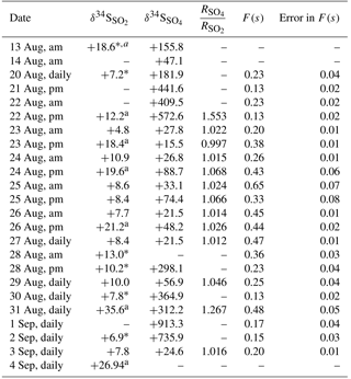
a tagged as enriched. * not blank corrected samples. These are only shown for comparison, no calculation has been done using these values.
Sulfate aerosols during CIMS-ON periods in the size ranges E0.49−0.95 µm, D0.95−1.5 µm, C1.5−3.0 µm, B3.0−7.2 µm, and A> 7.2 µm also showed enrichment for most of the samples (85 out of 100 samples showed enrichment; Table 3).
Table 3δ34S (‰) values for sulfate in size ranges E0.49−0.95 µm, D0.95−1.5 µm, C1.5−3.0 µm, B3.0−7.2 µm, and A> 7.2 µm during CIMS-ON periods. Average uncertainty for δ34S values is ±0.5 ‰.
* not blank corrected samples

Figure 9Sum of α-pinene, β-pinene, and Limonene versus ozone mixing ratio for daytime and nighttime and all data.
Since the CIMS exhaust was located to the southeast of the high-volume sampler, wind direction was considered as a potential factor in the analysis. No correlation (r = 0.16) was observed between the percent of time the high-volume sampler was downwind of the CIMS exhaust and the concentrations of 34SO2 or 34SO4.
5.4 The role of Criegee biradicals in SO2 oxidation
As mentioned in Sect. 5.1, F(s) was higher during the daytime in comparison to nighttime except for polluted periods. No correlation (r = −0.36, excluding 25 and 26 August with the highest RH) was observed between F(s) and the integrated OH production rate, suggesting that another oxidation pathway for SO2 was active during daytime. One likely pathway is oxidation of SO2 by Criegee biradicals.
Criegee biradicals are formed from ozonolysis of alkenes and may oxidize SO2 to sulfate increasing F(s) (Mauldin III et al., 2012). Therefore, it is expected that correlations may exist between F(s) and precursors to Criegee biradicals. Positive correlations between F(s) and the concentration of α-pinene (r = 0.85), β-pinene (r = 0.87), and limonene (r = 0.82) were observed during daytime (Fig. 8). However, no correlations were observed between F(s) and monoterpenes during nighttime.
The concentration of monoterpenes showed a negative correlation with the mixing ratio of O3. There was a power law relationship between monoterpenes and O3 mixing ratio during the daytime and a linear dependency at night (r = −0.60; Fig. 9).
Concentrations of other VOCs were only available as 24 h averages. Most of the alkenes measured were found to be below the detection limit. Alkenes with concentrations higher than the detection limit except isoprene showed significant positive correlations with secondary sulfate aerosols (D< 0.49 µm) and all of them except isoprene and tetrachloroethene showed significant correlations with SO2 (Table A2).
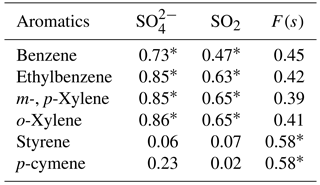
Correlations with aromatic compounds generally fell into two categories. The first set includes compounds which were highly correlated with SO2 and sulfate for impactor D< 0.49 µm (e.g., benzene). The second set contains the compounds which show no such correlations but were correlated with F(s) (Table A3). Styrene and p-cymene are two compounds with no correlation with SO2 and sulfate but significant correlations with F(s) (r = 0.58 for both, and r = 0.66 and r = 0.71, respectively, when the rainy day data are omitted, P value <0.05; Table A3, Fig. A6). They also show a positive correlation together (r = 0.71, P value < 0.05; Fig. A6).
6.1 Potential TMI-catalyzed SO2 oxidation
Sulfur conversion ratios (F(s)) and sulfur isotope data for SO2 and size-segregated sulfate aerosols were used to investigate the role of TMI-catalyzed SO2 oxidation in the region.
Figure 2 exhibits the expected correlation between F(s) and OH in daytime but not at night when aqueous phase reactions are important. The similar slopes for nighttime and daytime F(s) versus RH plots suggests that SO2 aqueous phase oxidation may be an important oxidation pathway for both day and night and the offset (intercept that is higher for daytime than nighttime) suggests there is additional gas phase SO2 oxidation that takes place during the day.
Known aqueous phase oxidants for SO2 are H2O2, O3, and O2 in the presence of TMIs (Herrmann et al., 2000). No correlation was observed between F(s) and O3 mixing ratios, which suggests that O3 is of minor importance as an oxidant in the aqueous phase. The pH dependency of aqueous O3 oxidation of SO2 makes this reaction very slow at low pH (pH < 5.5). This reaction is also self-limiting and production of sulfate lowers the pH and slows down further reaction (Seinfeld and Pandis, 1998). Therefore, aqueous phase oxidation of SO2 occurs mostly by H2O2 and/or O2 in the presence of TMIs.
The conversion ratio of SO2 to sulfate (F(s)) was higher during the day than at night except during polluted periods (14, 23, and 24 August). This is consistent with gas phase contributions to SO2 oxidation in addition to aqueous phase oxidation that occurred both during the day and at night (Sect. 5.1). On polluted nights, the SO2 to sulfate conversion ratio was twice as high as during the day and on 14 August at night the highest (0.77) conversion ratio for the entire campaign was observed (Tables 1 and 2). Averaged Fe and Mn concentrations on these polluted nights coincided with the highest values for SO2 to sulfate conversion (F(s); Fig. A3). Whenever both RH and the sum of Fe and Mn concentrations were high at night, the proportion of SO2 that was converted to sulfate (F(s)) was higher as well (Fig. 4). These conditions of coincident high RH and Fe + Mn concentrations was met on polluted nights during the campaign. On these nights the ratios of Fe ∕ Mn were around 40 (38, 40, 42 for 14, 23, 24 August, respectively). This specific ratio may be a useful indicator for the source of Fe and Mn in aerosols. A particular night that was not classified as polluted (21 August) was identified as having Fe and Mn from soil (Phillips-Smith et al., 2017). The ratio of Fe ∕ Mn on that night was 76, and the SO2 to sulfate conversion ratio was indistinguishable from the remainder of the non-polluted nighttime samples (Fig. 4). Therefore, it is reasonable to suggest that a Fe ∕ Mn value around 40 is associated with a non-soil source. The two remaining sources are upgrader emissions and haul road dust. This interpretation of Fe and Mn on polluted nights as originating from anthropogenic emissions (Fe ∕ Mn ∼ 40) rather than soil is consistent with the higher solubility of anthropogenic TMIs relative to soil (Kumar et al., 2010).
Sulfur isotope measurements can provide the means to distinguish TMI from H2O2 aqueous oxidation. Isotope fractionation will be evident in sulfate when a large reservoir of SO2 (e.g., from stack emissions) mixes with oxidants during transport and produces accumulated sulfate product captured over 12 or 24 h. So long as the fraction of reaction is low (< 30 %) the difference in δ34S values for SO2 and sulfate will reflect the magnitude and direction of the fractionation process. For the TMI-catalyzed pathway this direction is negative and produces lighter sulfate than SO2. This directly contrasts with fractionation for O3, H2O2, and OH oxidation pathways. Evidence that SO2 released from tall stacks is transported high above the ground and mixes down toward the surface at AMS 13 has been demonstrated by Gordon et al. (2017) and should provide conditions meeting the requirement for the fraction of reaction less than 30 % described here. The observed δ34S values for size-segregated sulfate aerosols in this study were consistent with aqueous TMI rather than H2O2 oxidation. Light δ34S values for sulfate aerosols were observed in the region in comparison to other potential atmospheric sulfur sources. An alternate explanation for isotopically light δ34S values in sulfate was proposed by Proemse et al. (2012b). Isotopically light δ34S values (−3.9 and +0.3 ‰) were reported by this group for sulfate from bulk and throughfall deposition (deposition of excess water onto the ground surface from wet leaves) in the Athabasca oil sands region, consistent with the observations in this study. Since these values were lighter than the potential sources in the region, this suggests a contribution of sulfate from a 34S depleted source. Proemse et al. (2012b) suggested that the low δ34S values observed for atmospheric sulfate collected at two sites were due to H2S emitted from tailing ponds. Tailing ponds were in close proximity to the two sites where low δ34S values were found. Proemse et al. (2012b) suggested that H2S was oxidized to SO2 and subsequently formed sulfate that then contributed to local sulfate deposition. The average value for δ34S of SO2 during CIMS-ON and CIMS-OFF (non enriched values) periods was +7.9 ± 2.1 ‰. This value is in the range of δ34S of primary sulfate from two major stacks (Proemse et al., 2012a). No negative values were observed for δ34S of SO2. If H2S was the main source of atmospheric sulfur, the opposite pattern to that observed in Fig. 5, is expected. The reason is that isotopically light SO2 from H2S oxidation is expected to produce secondary sulfate aerosols (from both homogeneous and heterogeneous reactions) in the smaller size fractions (F< 0.49 µm and E0.49−0.95 µm) with isotopically light δ34S values. The larger A> 7.2 µm and B3.0−7.2 µm size aerosols contain primary sulfate from soil and would reflect δ34S values for untreated oil sand (+6.4 ‰; Proemse et al., 2012a) in addition to sulfate from H2S oxidation so they would have progressively more positive δ34S values. Therefore, a discernable contribution of H2S to isotopically light samples through an SO2 oxidation pathway is ruled out.
Primary sulfate and SO2 can originate from haul road dust or diesel exhaust. δ34S values for these two sources are +5 ‰ and higher (Norman, 2004; Norman et al., 2004). Therefore, if haul road dust and diesel primary sulfate were transported with Fe and Mn, then δ34S values should converge to +5 ‰ or higher. This should be particularly evident for the larger size aerosols (A> 7.2 µm and B3.0−7.2 µm). In fact the opposite is observed in Fig. 5. Isotopically light δ34S values for sulfate aerosols in size ranges E0.49−0.95 µm, D0.95−1.5 µm, C1.5−3.0 µm, B3.0−7.2 µm, and A> 7.2 µm were observed during CIMS-OFF periods. These values indicate that there was no, or only a very small, contribution of primary sulfate from major stacks. This leaves SO2 from upgrader emissions as the most probable source of sulfate both for F< 0.49 µm size aerosols and for secondary sulfate formed on larger aerosol size fractions. δ34S values reflect isotope fractionation during oxidation of SO2 rather than source signatures. This is supported by a positive correlation between the sum of sulfate in size fractions F< 0.49 µm, E0.49−0.95 µm, D0.95−1.5 µm, and C1.5−3.0 µm and the concentrations of Fe and Mn and sum of Fe and Mn (r = 0.86, r = 0.89, and r = 0.86, respectively). The concentration of sulfate in size fractions F< 0.49 µm and E0.49−0.95 µm also showed positive correlations with the concentration of Fe and Mn. This indicates that when Fe and Mn were prevalent in aerosols, either more sulfate can be formed or Fe and Mn were transported to AMS 13 with SO2 from a common emission source, likely upgrader emissions. There were also anti-correlations between δ34S values of sulfate in size fraction F< 0.49 µm and the concentrations of Fe and Mn. This shows that lighter δ34S values were associated with secondary sulfate formation and higher concentrations of Fe and Mn. One possible explanation for these observations may be the TMI-catalyzed SO2 oxidation pathway during transport to the AMS 13 site.
6.2 CIMS-ON
Little 34SO2 reached the SO2 filter in the high-volume sampler since high sulfur isotope enrichment was not observed for SO2 samples (max 35.6 ‰). Instead 34SO2 was oxidized to sulfate either as it moved in the atmosphere or on the filters in the high-volume sampler. This result was unexpected since previous studies of δ34S for sulfate and SO2 showed no evidence of oxidation when SO2 passed through the filters under marine or continental conditions (Ghahremaninezhad et al., 2016). The lack of 34SO2 and the predominance of 34S molecules on sulfate aerosols demonstrates an oxidation pathway that is rapid and specific to the conditions at the ground level of the the AMS 13 site.
6.3 Potential oxidation of SO2 by Criegee biradicals
The proportion of sulfate from SO2 oxidation, F(s), during daytime is generally larger than F(s) at night (Tables 1 and 2). Greater vertical mixing is expected during the day than at night. Stack emissions high above ground (Gordon et al., 2017) undergo oxidation during transport to the AMS 13 site. Aloft, conventional oxidation pathways (i.e., OH-driven oxidation) are likely more important than near the surface. At the same time precursors to Criegee biradicals will be released and mixed upward. A larger F(s) during the day than at night suggests that during daytime gas phase SO2 oxidation occurs in addition to aqueous phase oxidation. Typically, OH is expected to dominate gas phase SO2 oxidation during the day. However, a correlation between F(s) and integrated OH production rate was not observed. Instead, positive correlations between F(s) and α-pinene, β-pinene and limonene were observed during the day but not at night (Fig. 8). This, combined with the loss of monoterpenes as daytime O3 mixing ratio increased, suggests Criegee biradicals may be an important factor in SO2 oxidation close to the surface during daytime. Monoterpenes are oxidized by O3 to form Criegee biradicals which can be stabilized and oxidize SO2 to form secondary sulfate. This pathway is potentially more important during the day but less so at night. At night, the emissions of monoterpenes continue into a shallow nocturnal boundary layer that is decoupled from the residual layer above it. The terpenes then titrate O3 at the surface, leading to the observed anti-correlation and low surface O3 mixing ratio which limits Criegee biradical production.
Reaction between O3 and anthropogenic alkenes may also generate Criegee biradicals, potentially leading to higher SO2 to sulfate conversion ratios (F(s)). Many anthropogenic alkenes and aromatics likely have sources in common with SO2 since a correlation (P value < 0.05) was observed between them (Tables A2 and A3). Their emissions are likely injected into (and transported within) layers above the measurement site and only sporadically entrain to the surface during daytime. When this happens, relationships between F(s) and anthropogenic alkenes may be observed. As an example, styrene and p-cymene did not correlate with SO2 or secondary sulfate but they were correlated with F(s) (r = 0.66, r = 0.71, respectively). Styrene and p-cymene were also highly correlated with each other (r = 0.71) suggesting they originated from the same source or sources. It is likely that styrene and p-cymene are indicators of other anthropogenic alkenes that facilitate SO2 oxidation (for instance, tetrachloroethene).
This is the first study to examine oxidation of SO2 as it is transported above and within the boundary layer at AMS 13, a highly polluted environment, during summer. Sulfur dioxide (SO2) and size-segregated sulfate aerosol concentrations and sulfur isotope compositions were measured during summer 2013 in the Athabasca oil sands region to investigate SO2 oxidation pathways.
δ34S values, F(s), and the relationship between secondary sulfate concentrations and Fe and Mn (in PM2.5) show that there is the potential that a significant proportion of SO2 is oxidized rapidly during both the day and at night. Aqueous phase oxidation by TMI catalysis is consistent with these results. The fraction of secondary sulfate was higher during the night than during the day for periods when the site was impacted by industrial plumes mixing downward from above. This, taken together with the high Fe and Mn concentrations in PM2.5 at night, shows the importance of aqueous phase reactions, probably by the TMI pathway as SO2 is transported from the stack to the site at night. In addition, a natural tracer experiment with enriched 34S demonstrated that oxidation of SO2 on the surface of aerosols is rapid. The results would be consistent with Criegee biradicals being an important daytime oxidation pathway for SO2 at ground level, which was suggested in several recent high-profile papers (Mauldin III et al., 2012; Boy et al., 2013; Sipilä et al., 2014).
All data are available at ftp://arqpftp:research@ftp.tor.ec.gc.ca/OS/AMS13, last access: 10 October 2017.
Table A1The fraction of enriched 34S in sulfate samples in the size range F< 0.49 µm and the number of enriched sulfur molecules cm−3 for SO2 and sulfate during CIMS-ON periods.
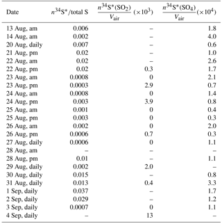
Table A2Correlation coefficients (r) between SO2, sulfate, and alkenes with concentrations higher than the detection limit. P values < 0.05 are indicated with a *.
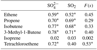
* P values < 0.05.
Table A3Correlation coefficients (r) between selected aromatics (at least 15 out of 20 data points are above the detection limit), SO2, and sulfate. P values < 0.05 are indicated with a *.
* P values < 0.05.

Figure A1(a) Temperature and relative humidity data with 1 min sampling interval. (b) Wind speed and wind direction with the sampling time interval of 5 min (data from WBEA meteorological station AMS 13). The gray shaded areas show the CIMS-ON periods.
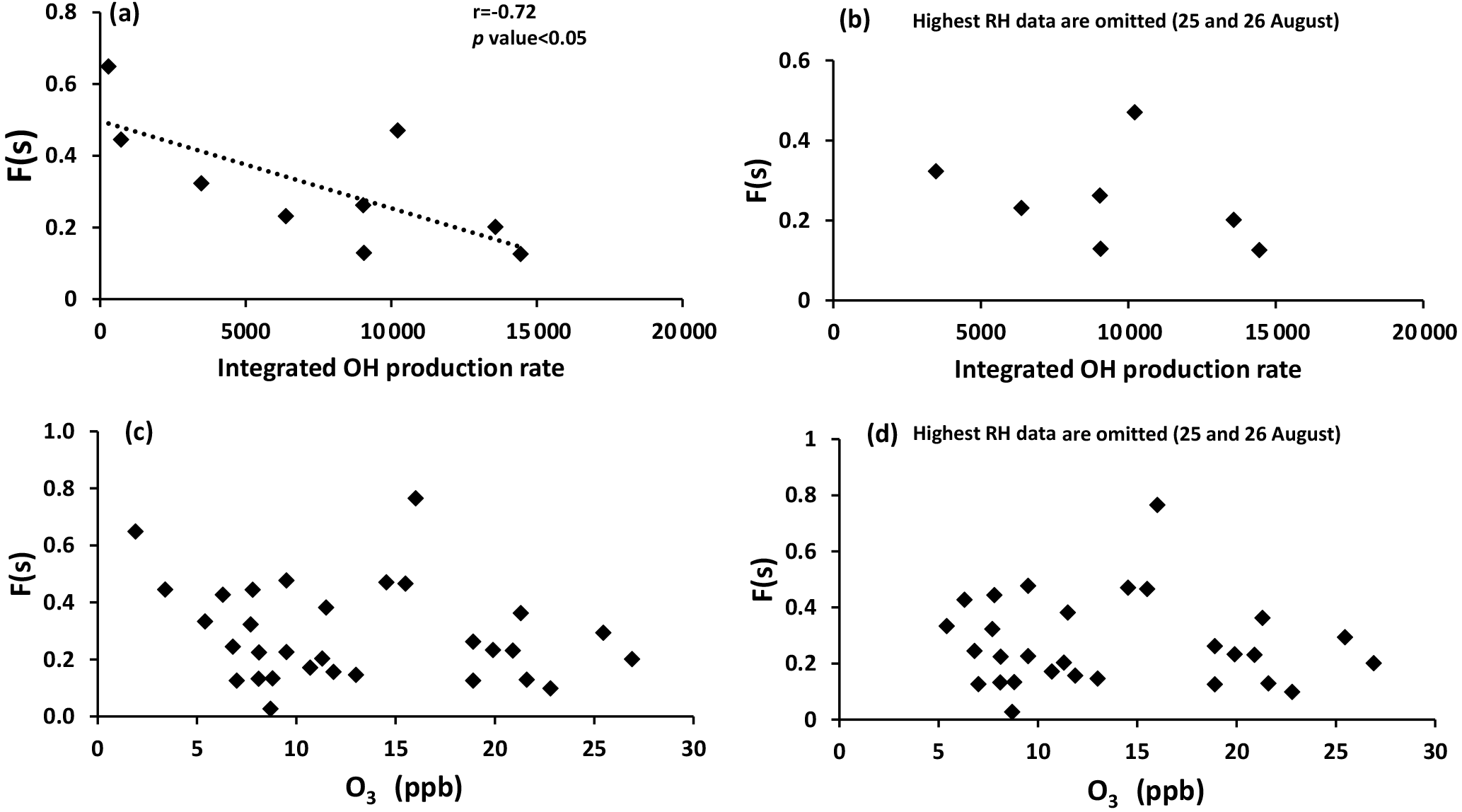
Figure A2Sulfur conversion ratio F(s) versus (a) integrated OH production rate for all available daytime data, (b) integrated OH production rate when 25 and 26 August data with highest RH are omitted, (c) O3 with daytime, nighttime, and daily data, and (d) O3 with all data when 25 and 26 August data with highest RH are omitted.
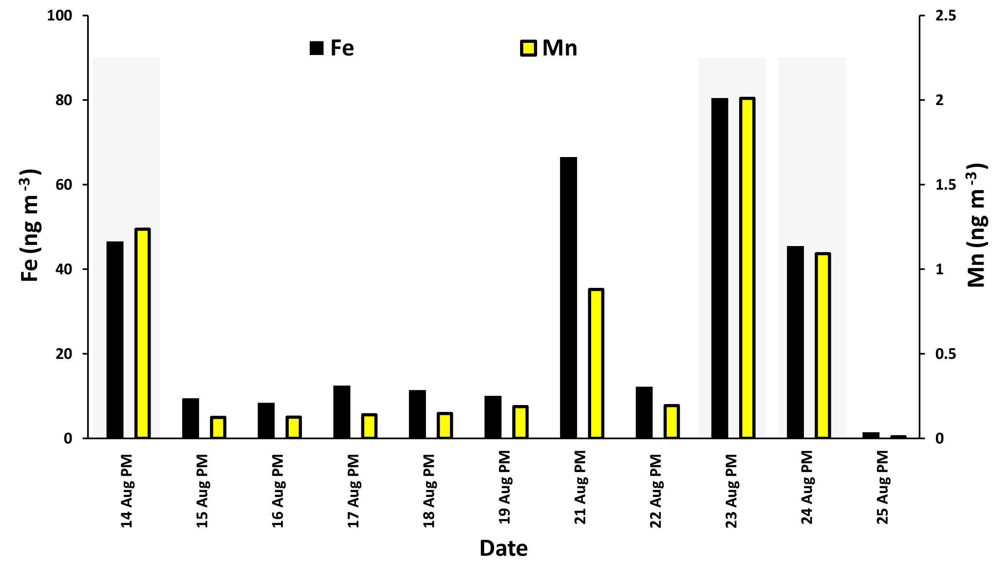
Figure A3Concentrations of Fe and Mn during nighttime (PM) averaged during the high-volume sampler running periods.
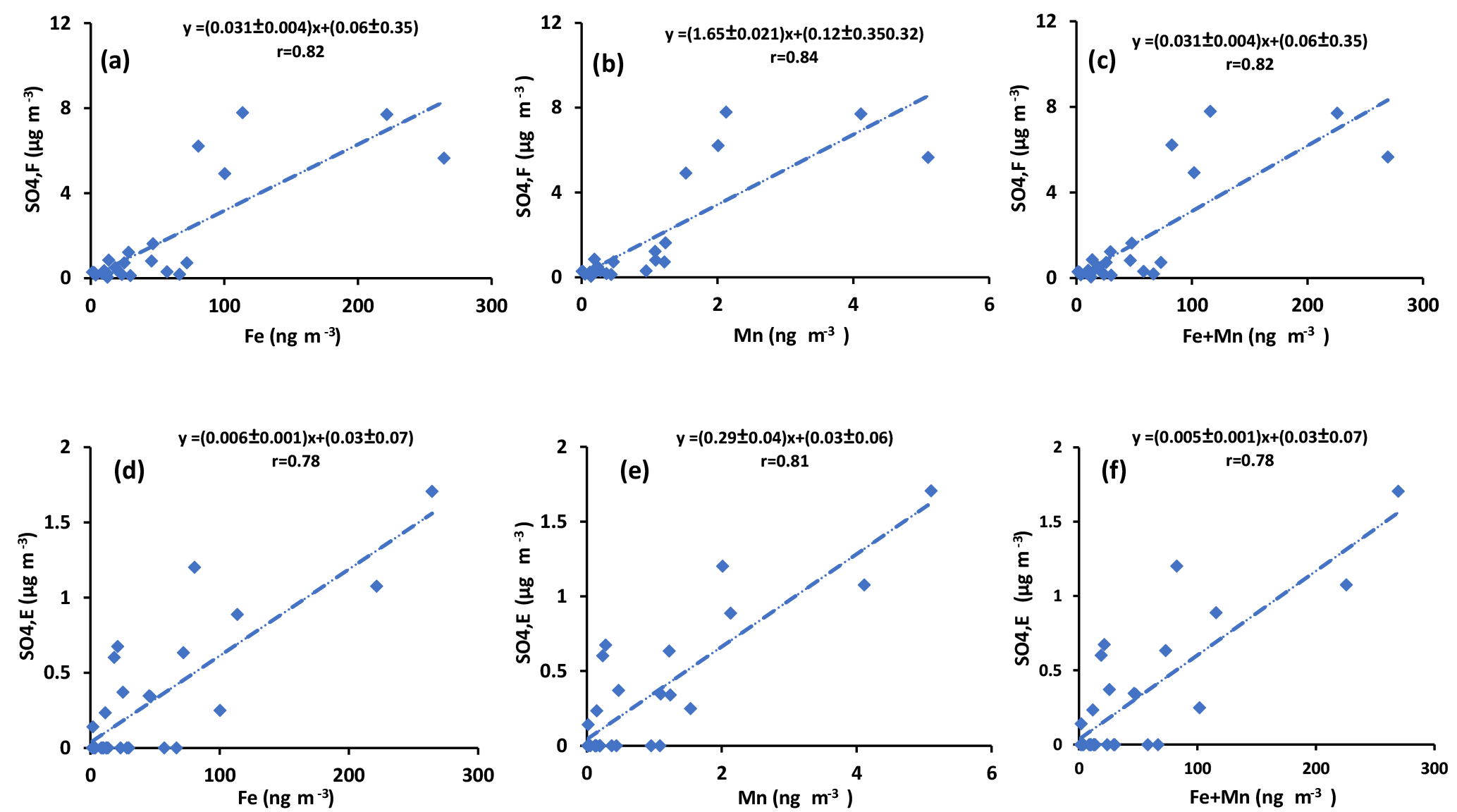
Figure A4(a–c) SO4 in size fraction F< 0.49 µm versus the concentrations of Fe and Mn measured in PM2.5 and the addition of Fe and Mn. (d–f) SO4 in size fraction E0.49−0.95 µm versus the concentrations of Fe and Mn measured in PM2.5 and the addition of Fe and Mn.

Figure A5Concentrations of (a) Fe and (b) Mn measured in PM2.5 versus the concentration of SO2.
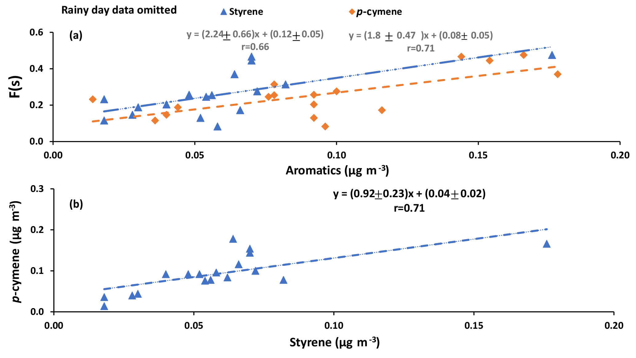
Figure A6(a) F(s) versus the concentration of styrene and p-cymene (b) p-cymene versus styrene.
The authors declare that they have no conflict of interest.
This article is part of the special issue “Atmospheric emissions from oil sands development and their transport, transformation and deposition (ACP/AMT inter-journal SI)”. It is not associated with a conference.
This project was funded by Environment Canada under the Joint Canada-Alberta
Implementation Plan for Oil Sands Monitoring (JOSM) and NSERC. We would like
to thank Jeff Brook and Daniel Wang from Environment Canada for VOC
measurements and Greg Evans and Cheol-Heon Jeong from the University of Toronto
for their data on Fe and Mn concentrations. We also thank Jeremy Wentzell
from Environment Canada for his assistance in defining working periods of
CIMS.
Edited by: Shao-Meng Li
Reviewed by: three anonymous referees
Bardouki, H., Berresheim, H., Vrekoussis, M., Sciare, J., Kouvarakis, G., Oikonomou, K., Schneider, J., and Mihalopoulos, N.: Gaseous (DMS, MSA, SO2, H2SO4 and DMSO) and particulate (sulfate and methanesulfonate) sulfur species over the northeastern coast of Crete, Atmos. Chem. Phys., 3, 1871–1886, https://doi.org/10.5194/acp-3-1871-2003, 2003. a
Benson, D. R., Young, L.-H., Kameel, F. R., and Lee, S.-H.: Laboratory-measured nucleation rates of sulfuric acid and water binary homogeneous nucleation from the SO2+OH reaction, Geophys. Res. Lett., 35, L11801, https://doi.org/10.1029/2008GL033387, 2008. a
Berglen, T. F.: A global model of the coupled sulfur/oxidant chemistry in the troposphere: The sulfur cycle, J. Geophys. Res., 109, D19310, https://doi.org/10.1029/2003JD003948, 2004. a
Berndt, T., Jokinen, T., Mauldin, R. L., Petäjä, T., Herrmann, H., Junninen, H., Paasonen, P., Worsnop, D. R., and Sipilä, M.: Gas-Phase Ozonolysis of Selected Olefins: The Yield of Stabilized Criegee Intermediate and the Reactivity toward SO2, J. Phys. Chem. Lett., 3, 2892–2896, https://doi.org/10.1021/jz301158u, 2012. a
Berresheim, H.: Gas-aerosol relationships of H2SO4 , MSA, and OH: Observations in the coastal marine boundary layer at Mace Head, Ireland, J. Geophys. Res., 107, 8100, https://doi.org/10.1029/2000JD000229, 2002. a
Berresheim, H., Wine, P., and Davis, D.: Sulfur in the atmosphere, in Composition, Chemistry, and Climate of the Atmosphere, Van Nostrand Reinhold, New York, 251–307, 1995. a
Boucher, O. and Lohmann, U.: The sulfate-CCN-cloud albedo effect., Tellus B, 47, 281–300, https://doi.org/10.1034/j.1600-0889.47.issue3.1.x, 1995. a
Boy, M., Mogensen, D., Smolander, S., Zhou, L., Nieminen, T., Paasonen, P., Plass-Dülmer, C., Sipilä, M., Petäjä, T., Mauldin, L., Berresheim, H., and Kulmala, M.: Oxidation of SO2 by stabilized Criegee intermediate (sCI) radicals as a crucial source for atmospheric sulfuric acid concentrations, Atmos. Chem. Phys., 13, 3865–3879, https://doi.org/10.5194/acp-13-3865-2013, 2013. a, b, c
Brimblecombe, P., Hammer, C., Rodhe, H., Ryaboshapko, A., and Boutron, C. F.: Human influence on the sulfur cycle. In Evolution of the Global Biogeochemical Sulphur Cycle, Wiley, Chichester, 39, 77–121, 1989. a
Burkholder, J. B., Sander, S. P., Abbatt, J., Barker, J. R., Huie, R. E., Kolb, C. E., Kurylo, M. J., Orkin, V. L., Wilmouth, D. M., and Wine, P. H.: Chemical Kinetics and Photochemical Data for Use in Atmospheric Studies, Evaluation Number 18, Tech. Rep. 15, Jet Propulsion Laboratory, Pasadena, available at: http://jpldataeval.jpl.nasa.gov (last access: 10 October 2017), 2015. a
Chin, M. and Jacob, D. J.: Anthropogenic and natural contributions to tropospheric sulfate: A global model analysis, J. Geophys. Res.-Atmos., 101, 18691–18699, https://doi.org/10.1029/96JD01222, 1996. a, b, c
Chin, M., Rood, R. B., Lin, S.-J., Müller, J.-F., and Thompson, A. M.: Atmospheric sulfur cycle simulated in the global model GOCART: Model description and global properties, J. Geophys. Res.-Atmos., 105, 24671–24687, https://doi.org/10.1029/2000JD900384, 2000. a, b
Ding, T., Valkiers, S., Kipphardt, H., De Bièvre, P., Taylor, P., Gonfiantini, R., and Krouse, R.: Calibrated sulfur isotope abundance ratios of three IAEA sulfur isotope reference materials and V-CDT with a reassessment of the atomic weight of sulfur, Geochim. Cosmochim. Ac., 65, 2433–2437, https://doi.org/10.1016/S0016-7037(01)00611-1, 2001. a
Eriksen, T. E., Vikane, O., Swahn, C.-G., Larsson, R., Nordén, B., and Sundbom, M.: Sulfur Isotope Effects I. The Isotopic Exchange Coefficient for the Sulfur Isotopes 34S-32S in the System SO2 g- aq at 25, 35, and 45 ∘C, Acta Chem. Scand., 26, 573–580, https://doi.org/10.3891/acta.chem.scand.26-0573, 1972. a
Fioletov, V. E., McLinden, C. A., Cede, A., Davies, J., Mihele, C., Netcheva, S., Li, S.-M., and O'Brien, J.: Sulfur dioxide (SO2) vertical column density measurements by Pandora spectrometer over the Canadian oil sands, Atmos. Meas. Tech., 9, 2961–2976, https://doi.org/10.5194/amt-9-2961-2016, 2016. a
Gerhardsson, L.: Acid precipitation - effects on trace elements and human health, Sci. Total Environ., 153, 237–245, 1994. a
Ghahremaninezhad, R., Norman, A.-L., Abbatt, J. P. D., Levasseur, M., and Thomas, J. L.: Biogenic, anthropogenic and sea salt sulfate size-segregated aerosols in the Arctic summer, Atmos. Chem. Phys., 16, 5191–5202, https://doi.org/10.5194/acp-16-5191-2016, 2016. a
Giesemann, A., Jaeger, H.-J., Norman, A. L., Krouse, H. R., and Brand, W. A.: Online Sulfur-Isotope Determination Using an Elemental Analyzer Coupled to a Mass Spectrometer, Anal. Chem., 66, 2816–2819, https://doi.org/10.1021/ac00090a005, 1994. a
Gordon, M., Makar, P. A., Staebler, R. M., Zhang, J., Akingunola, A., Gong, W., and Li, S.-M.: A Comparison of Plume Rise Algorithms to Stack Plume Measurements in the Athabasca Oil Sands, Atmos. Chem. Phys. Discuss., https://doi.org/10.5194/acp-2017-1093, in review, 2017. a, b
Hains, J. C.: A chemical climatology of lower tropospheric trace gases and aerosols over themid-atlanticregion (doctoral dissertation), PhD thesis, University of Maryland, 2007. a
Harris, E., Sinha, B., Hoppe, P., Crowley, J. N., Ono, S., and Foley, S.: Sulfur isotope fractionation during oxidation of sulfur dioxide: gas-phase oxidation by OH radicals and aqueous oxidation by H2O2, O3 and iron catalysis, Atmos. Chem. Phys., 12, 407–423, https://doi.org/10.5194/acp-12-407-2012, 2012. a, b, c, d
Harris, E., Sinha, B., Hoppe, P., and Ono, S.: High-Precision Measurements of 33S and 34S Fractionation during SO2 Oxidation Reveal Causes of Seasonality in SO2 and Sulfate Isotopic Composition, Environ. Sci. Technol., 47, 12174–12183, https://doi.org/10.1021/es402824c, 2013a. a, b
Harris, E., Sinha, B., van Pinxteren, D., Tilgner, A., Fomba, K. W., Schneider, J., Roth, A., Gnauk, T., Fahlbusch, B., Mertes, S., Lee, T., Collett, J., Foley, S., Borrmann, S., Hoppe, P., and Herrmann, H.: Enhanced Role of Transition Metal Ion Catalysis During In-Cloud Oxidation of SO2, Science, 340, 727–730, https://doi.org/10.1126/science.1230911, 2013b. a
Hegg, D. A., Covert, D. S., Jonsson, H., Khelif, D., and Friehe, C. A.: Observations of the impact of cloud processing on aerosol light-scattering efficiency, Tellus B, 56, 285–293, 2004. a
Herrmann, H., Ervens, B., Jacobi, H.-W., Wolke, R., Nowacki, P., and Zellner, R.: CAPRAM2.3: A Chemical Aqueous Phase Radical Mechanism for Tropospheric Chemistry, J. Atmos. Chem., 36, 231–284, https://doi.org/10.1023/A:1006318622743, 2000. a, b, c
Hicks, B.: Dry deposition to forests – On the use of data from clearings, Agric. For. Meteorol., 136, 214–221, https://doi.org/10.1016/j.agrformet.2004.06.013, 2006. a
Howell, S. G., Clarke, A. D., Freitag, S., McNaughton, C. S., Kapustin, V., Brekovskikh, V., Jimenez, J.-L., and Cubison, M. J.: An airborne assessment of atmospheric particulate emissions from the processing of Athabasca oil sands, Atmos. Chem. Phys., 14, 5073–5087, https://doi.org/10.5194/acp-14-5073-2014, 2014. a
IPCC2001: Climate Change 2001: The Scientific Basis. Contribution of Working Group I to the Third Assessment Report of the Intergovermental Panel on Climate Change, Tech. rep., Cambridge University Press, 2001. a
Jacob, D. J. and Hoffmann, M. R.: A dynamic model for the production of , and in urban fog, J. Geophys. Res., 88, 6611, https://doi.org/10.1029/JC088iC11p06611, 1983. a
Jacob, D. J., Waldman, J. M., Munger, J. W., and Hoffmann, M. R.: A field investigation of physical and chemical mechanisms affecting pollutant concentrations in fog droplets, Tellus B, 36B, 272–285, 1984. a
Jacob, D. J., Gottlieb, E. W., and Prather, M. J.: Chemistry of a polluted cloudy boundary layer, J. Geophys. Res., 94, 12975, https://doi.org/10.1029/JD094iD10p12975, 1989. a
Kindzierski, W. B. and Ranganathan, H. K.: Indoor and outdoor SO2 in a community near oil sand extraction and production facilities in northern Alberta, J. Environ. Eng. Sci., 5, S121–S129, https://doi.org/10.1139/s06-022, 2006. a
Krouse, H. and Grinenko, V.: SCOPE 43, John Wiley and Sons, Chichester, New York, Brisbane, Toronto, Singapore, Scientific Committee on Problems of the Environment, 1991. a
Kulmala, M., Vehkamäki, H., Petäjä, T., Dal Maso, M., Lauri, A., Kerminen, V.-M., Birmili, W., and McMurry, P.: Formation and growth rates of ultrafine atmospheric particles: a review of observations, J. Aerosol Sci., 35, 143–176, https://doi.org/10.1016/j.jaerosci.2003.10.003, 2004. a, b
Kulmala, M., Riipinen, I., Sipila, M., Manninen, H. E., Petaja, T., Junninen, H., Maso, M. D., Mordas, G., Mirme, A., Vana, M., Hirsikko, A., Laakso, L., Harrison, R. M., Hanson, I., Leung, C., Lehtinen, K. E. J., and Kerminen, V.-M.: Toward Direct Measurement of Atmospheric Nucleation, Science, 318, 89–92, https://doi.org/10.1126/science.1144124, 2007. a
Kumar, A., Sarin, M., and Srinivas, B.: Aerosol iron solubility over Bay of Bengal: Role of anthropogenic sources and chemical processing, Mar. Chem., 121, 167–175, https://doi.org/10.1016/j.marchem.2010.04.005, 2010. a
Liggio, J., Li, S.-M., Hayden, K., Taha, Y. M., Stroud, C., Darlington, A., Drollette, B. D., Gordon, M., Lee, P., Liu, P., Leithead, A., Moussa, S. G., Wang, D., O'Brien, J., Mittermeier, R. L., Brook, J. R., Lu, G., Staebler, R. M., Han, Y., Tokarek, T. W., Osthoff, H. D., Makar, P. A., Zhang, J., L. Plata, D., and Gentner, D. R.: Oil sands operations as a large source of secondary organic aerosols, Nature, 534, 91–94, https://doi.org/10.1038/nature17646, 2016. a
Lin, M., Biglari, S., and Thiemens, M. H.: Quantification of Gas-to-Particle Conversion Rates of Sulfur in the Terrestrial Atmosphere Using High-Sensitivity Measurements of Cosmogenic 35S, ACS Earth Sp. Chem., 1, 324–333, https://doi.org/10.1021/acsearthspacechem.7b00047, 2017. a
Mauldin III, R. L., Berndt, T., Sipilä, M., Paasonen, P., Petäjä, T., Kim, S., Kurtén, T., Stratmann, F., Kerminen, V.-M., and Kulmala, M.: A new atmospherically relevant oxidant of sulphur dioxide, Nature, 488, 193–196, https://doi.org/10.1038/nature11278, 2012. a, b, c, d, e
McCabe, J. R., Savarino, J., Alexander, B., Gong, S., and Thiemens, M. H.: Isotopic constraints on non-photochemical sulfate production in the Arctic winter, Geophys. Res. Lett., 33, L05810, https://doi.org/10.1029/2005GL025164, 2006. a
McLinden, C. A., Fioletov, V., Boersma, K. F., Krotkov, N., Sioris, C. E., Veefkind, J. P., and Yang, K.: Air quality over the Canadian oil sands: A first assessment using satellite observations, Geophys. Res. Lett., 39, L04804, https://doi.org/10.1029/2011GL050273, 2012. a
Mertes, S., Galgon, D., Schwirn, K., Nowak, A., Lehmann, K., Massling, A., Wiedensohler, A., and Wieprecht, W.: Evolution of particle concentration and size distribution observed upwind, inside and downwind hill cap clouds at connected flow conditions during FEBUKO, Atmos. Environ., 39, 4233–4245, https://doi.org/10.1016/j.atmosenv.2005.02.009, 2005a. a
Mertes, S., Lehmann, K., Nowak, A., Massling, A., and Wiedensohler, A.: Link between aerosol hygroscopic growth and droplet activation observed for hill-capped clouds at connected flow conditions during FEBUKO, Atmos. Environ., 39, 4247–4256, https://doi.org/10.1016/j.atmosenv.2005.02.010, 2005b. a
Myles, L., Meyers, T. P., and Robinson, L.: Relaxed eddy accumulation measurements of ammonia, nitric acid, sulfur dioxide and particulate sulfate dry deposition near Tampa, FL, USA, Environ. Res. Lett., 2, 034004, https://doi.org/10.1088/1748-9326/2/3/034004, 2007. a
Newman, L., Krouse, H. R., and Grinenko, V. A.: Sulphur isotope variations in the atmosphere, John Wiley and Sons, United Kingdom, 1991. a
Norman, A.: Insights into the biogenic contribution to total sulphate in aerosol and precipitation in the Fraser Valley afforded by isotopes of sulphur and oxygen, J. Geophys. Res., 109, D05311, https://doi.org/10.1029/2002JD003072, 2004. a, b, c, d
Norman, A., Krouse, H., and Macleod, J.: Apportionment of Pollutants in an Urban Airshed: Calgary, Canada, A Case Study, in: Air Pollution Modeling and its Application XVI, edited by Carlos, B. and Incecik, S., 107–125, Springer US, https://doi.org/10.1007/978-1-4419-8867-6, 2004. a, b
Odame-Ankrah, C. A.: Improved Detection Instrument for Nitrogen Oxide Species, Ph.D. thesis, University of Calgary, available at: http://hdl.handle.net/11023/2006 (last access: 10 October 2017), 2015. a
Osthoff, H. D., Odame-Ankrah, C. A., Taha, Y. M., Tokarek, T. W., Schiller, C. L., Haga, D., Jones, K., and Vingarzan, R.: Low levels of nitryl chloride at ground level: nocturnal nitrogen oxides in the Lower Fraser Valley of British Columbia, Atmos. Chem. Phys., 18, 6293–6315, https://doi.org/10.5194/acp-18-6293-2018, 2018. a
Paul, D. and Osthoff, H. D.: Absolute Measurements of Total Peroxy Nitrate Mixing Ratios by Thermal Dissociation Blue Diode Laser Cavity Ring-Down Spectroscopy, Anal. Chem., 82, 6695–6703, https://doi.org/10.1021/ac101441z, 2010. a
Percy, K. E.: Geoscience of Climate and Energy 11. Ambient Air Quality and Linkage to Ecosystems in the Athabasca Oil Sands, Alberta, Geosci. Canada, 40, 182, https://doi.org/10.12789/geocanj.2013.40.014, 2013. a
Phillips-Smith, C., Jeong, C.-H., Healy, R. M., Dabek-Zlotorzynska, E., Celo, V., Brook, J. R., and Evans, G.: Sources of particulate matter components in the Athabasca oil sands region: investigation through a comparison of trace element measurement methodologies, Atmos. Chem. Phys., 17, 9435–9449, https://doi.org/10.5194/acp-17-9435-2017, 2017. a, b, c, d, e, f, g, h, i
Proemse, B. C., Mayer, B., Chow, J. C., and Watson, J. G.: Isotopic characterization of nitrate, ammonium and sulfate in stack PM2.5 emissions in the Athabasca Oil Sands Region, Alberta, Canada, Atmos. Environ., 60, 555–563, https://doi.org/10.1016/j.atmosenv.2012.06.046, 2012a. a, b, c, d, e, f
Proemse, B. C., Mayer, B., and Fenn, M. E.: Tracing industrial sulfur contributions to atmospheric sulfate deposition in the Athabasca oil sands region, Alberta, Canada, Appl. Geochem., 27, 2425–2434, https://doi.org/10.1016/j.apgeochem.2012.08.006, 2012b. a, b, c
Puig, R., Àvila, A., and Soler, A.: Sulphur isotopes as tracers of the influence of a coal-fired power plant on a Scots pine forest in Catalonia (NE Spain), Atmos. Environ., 42, 733–745, https://doi.org/10.1016/j.atmosenv.2007.09.059, 2008. a
Sanusi, A. A., Norman, A.-L., Burridge, C., Wadleigh, M., and Tang, W.-W.: Determination of the S Isotope Composition of Methanesulfonic Acid, Anal. Chem., 78, 4964–4968, https://doi.org/10.1021/ac0600048, 2006. a
Seinfeld, J. H. and Pandis, S. N.: Atmospheric Chemistry and Physics: From Air Pollution to Climate Change, Wiley and Sons, New York, USA, 1998. a, b, c
Simpson, I. J., Blake, N. J., Barletta, B., Diskin, G. S., Fuelberg, H. E., Gorham, K., Huey, L. G., Meinardi, S., Rowland, F. S., Vay, S. A., Weinheimer, A. J., Yang, M., and Blake, D. R.: Characterization of trace gases measured over Alberta oil sands mining operations: 76 speciated C2–C10 volatile organic compounds (VOCs), CO2, CH4, CO, NO, NO2, NOy, O3 and SO2, Atmos. Chem. Phys., 10, 11931–11954, https://doi.org/10.5194/acp-10-11931-2010, 2010. a
Sipilä, M., Jokinen, T., Berndt, T., Richters, S., Makkonen, R., Donahue, N. M., Mauldin III, R. L., Kurtén, T., Paasonen, P., Sarnela, N., Ehn, M., Junninen, H., Rissanen, M. P., Thornton, J., Stratmann, F., Herrmann, H., Worsnop, D. R., Kulmala, M., Kerminen, V.-M., and Petäjä, T.: Reactivity of stabilized Criegee intermediates (sCIs) from isoprene and monoterpene ozonolysis toward SO2 and organic acids, Atmos. Chem. Phys., 14, 12143–12153, https://doi.org/10.5194/acp-14-12143-2014, 2014. a, b
Sjostedt, S., Huey, L., Tanner, D., Peischl, J., Chen, G., Dibb, J., Lefer, B., Hutterli, M., Beyersdorf, A., Blake, N., Blake, D., Sueper, D., Ryerson, T., Burkhart, J., and Stohl, A.: Observations of hydroxyl and the sum of peroxy radicals at Summit, Greenland during summer 2003, Atmos. Environ., 41, 5122–5137, https://doi.org/10.1016/j.atmosenv.2006.06.065, 2007. a
Soares, J., Makar, P. A., Aklilu, Y., and Akingunola, A.: The use of hierarchical clustering for the design of optimized monitoring networks, Atmos. Chem. Phys., 18, 6543–6566, https://doi.org/10.5194/acp-18-6543-2018, 2018. a
Sofen, E. D., Alexander, B., and Kunasek, S. A.: The impact of anthropogenic emissions on atmospheric sulfate production pathways, oxidants, and ice core Δ17O(), Atmos. Chem. Phys., 11, 3565–3578, https://doi.org/10.5194/acp-11-3565-2011, 2011. a
Tanaka, N., Rye, D. M., Xiao, Y., and Lasaga, A. C.: Use of stable sulfur isotope systematics for evaluating oxidation reaction pathways and in-cloud-scavenging of sulfur dioxide in the atmosphere, Geophys. Res. Lett., 21, 1519–1522, https://doi.org/10.1029/94GL00893, 1994. a
Tokarek, T. W., Brownsey, D. K., Jordan, N., Garner, N. M., Ye, C. Z., Assad, F. V., Peace, A., Schiller, C. L., Mason, R. H., Vingarzan, R., and Osthoff, H. D.: Biogenic Emissions and Nocturnal Ozone Depletion Events at the Amphitrite Point Observatory on Vancouver Island, Atmos. Ocean, 55, 121–132, https://doi.org/10.1080/07055900.2017.1306687, 2017. a
Twomey, S.: Aerosols, clouds and radiation, Atmos. Environ. Part A. Gen. Top., 25, 2435–2442, https://doi.org/10.1016/0960-1686(91)90159-5, 1991. a
Wadleigh, M. and Blake, D.: Tracing sources of atmospheric sulphur using epiphytic lichens, Environ. Pollut., 106, 265–271, https://doi.org/10.1016/S0269-7491(99)00114-1, 1999. a
Welz, O., Savee, J. D., Osborn, D. L., Vasu, S. S., Percival, C. J., Shallcross, D. E., and Taatjes, C. A.: Direct Kinetic Measurements of Criegee Intermediate (CH2OO) Formed by Reaction of CH2I with O2, Science, 335, 204–207, https://doi.org/10.1126/science.1213229, 2012. a
Yuskiewicz, B. A., Stratmann, F., Birmili, W., Wiedensohler, A., Swietlicki, E., Berg, O., and Zhou, J.: The effects of in-cloud mass production on atmospheric light scatter, Atmos. Res., 50, 265–288, https://doi.org/10.1016/S0169-8095(98)00107-0, 1999. a