Decrease in tropospheric O₃ levels in the Northern Hemisphere observed by IASI

In this study, we describe the recent changes in the tropospheric ozone (O₃) columns measured by the Infrared Atmospheric Sounding Interferometer (IASI), onboard the Metop satellite, during the first 9 years of operation (January 2008 to May 2017). Using appropriate multivariate regression methods, we differentiate significant linear trends from other sources of O₃ variations captured by IASI. The geographical patterns of the adjusted O₃ trends are provided and discussed on the global scale. Given the large contribution of the natural variability in comparison with that of the trend (25–85 % vs. 15–50 %, respectively) to the total O₃ variations, we estimate that additional years of IASI measurements are generally required to detect the estimated O₃ trends with high precision. Globally, additional 6 months to 6 years of measurements, depending on the regions and the seasons, are needed to detect a trend of $\left|\mathrm{5}\right|$ DU decade⁻¹. An exception is interestingly found during summer at mid- and high latitudes of the Northern Hemisphere (NH; ∼ 40 to ∼ 75^∘ N), where the large absolute fitted trend values (∼ $\left|\mathrm{0.5}\right|$ DU yr⁻¹ on average) combined with the small model residuals (∼ 10 %) allow for detection of a band-like pattern of significant negative trends. Despite no consensus in terms of tropospheric O₃ trends having been reached from the available independent datasets (UV or IR satellites, O₃ sondes, aircrafts, ground-based measurements, etc.) for the reasons that are discussed in the text, this finding is consistent with the reported decrease in O₃ precursor emissions in recent years, especially in Europe and USA. The influence of continental pollution on that latitudinal band is further investigated and supported by the analysis of the O₃–CO relationship (in terms of correlation coefficient, regression slope and covariance) that we found to be the strongest at northern midlatitudes in summer.

1 Introduction

O₃ plays a key role throughout the whole troposphere where it is produced by the photochemical oxidation of carbon monoxide (CO), non-methane volatile organic compounds (NMVOCs) and methane (CH₄) in the presence of nitrogen oxides (NO_x) (e.g., Logan et al., 1981). O₃ sources in the troposphere consist of the in situ photochemical production from anthropogenic and natural precursors and the downwards transport of stratospheric O₃. Being a strong pollutant, a major reactive species and an important greenhouse gas in the upper troposphere, O₃ is of greatest interest regarding air quality, atmospheric chemistry and radiative forcing studies. Thanks to its long lifetime (several weeks) relative to transport timescales in the free troposphere (Fusco and Logan, 2003), O₃ also contributes to large-scale transport of pollution far from source regions with further impacts on global air quality (e.g., Stohl et al., 2002; Parrish et al., 2012) and climate. Monitoring and understanding the time evolution of tropospheric O₃ at a global scale is, therefore, crucial to apprehend future climate changes. Nevertheless, a series of limitations make O₃ trends particularly challenging to retrieve and to interpret.

While the O₃ precursors anthropogenic emissions have increased and shifted equatorward in the developing countries (Zhang et al., 2016) since the 1980s, extensive campaigns and routine in situ and remote measurements at specific urban and rural sites have provided long-term but sparse datasets of tropospheric O₃ (e.g., Cooper et al., 2014 and references therein). Ultraviolet and visible (UV/VIS) atmospheric sounders onboard satellites provide tropospheric O₃ measurements with much wider coverage, but they result either from indirect methods (e.g., Fishman et al., 2005) or from direct retrievals which are limited by coarse vertical resolution (Liu et al., 2010). All these datasets also suffer from a lack of homogeneity in terms of measurement methods (instrument and algorithm) and spatio-temporal samplings (e.g., Doughty et al., 2011; Heue et al., 2016; Leventidou et al., 2017). Those limitations, in addition to the large natural interannual variability (IAV) and decadal variations in tropospheric O₃ levels (due to large-scale dynamical modes of O₃ variations and to changes in stratospheric O₃, in stratosphere–troposphere exchanges, in precursor emissions and in their geographical patterns), introduce strong biases in trends determined from independent studies and datasets (e.g., Zbinden et al., 2006; Thouret et al., 2006; Logan et al., 2012; Parrish et al., 2012 and references therein). As a consequence, determining accurate trends requires a long period of high density and homogeneous measurements (e.g., Payne et al., 2017).

Such long-term datasets are now becoming obtainable with the new generation of nadir-looking and polar-orbiting instruments measuring in the thermal infrared region. In particular, about one decade of O₃ profile measurements, with good sensitivity in the troposphere independent from the layers above, is now available from the IASI (Infrared Atmospheric Sounding Interferometer) sounder aboard the European Metop platforms, allowing the monitoring of regional and global variations in tropospheric O₃ levels (e.g., Dufour et al., 2012; Safieddine et al., 2014; Wespes et al., 2016).

In this study, we examine the tropospheric O₃ changes behind the natural IAV as measured by IASI over January 2008–May 2017. To that end, we use the approach described in Wespes et al. (2017), which relies on a multi-linear regression (MLR) procedure, for accurately differentiating trends from other sources of O₃ variations, the latter being robustly identified and quantified in the companion study. In Sect. 2, we briefly review the IASI mission and the tropospheric O₃ product, and we shortly describe the multivariate models (annual or seasonal) that we use for fitting the daily O₃ time series. In Sect. 3, after verifying the performance of the MLR models over the available IASI dataset, we evaluate the feasibility of capturing and retrieving significant trend parameters, apart from natural O₃ dependencies, by performing trend sensitivity studies. In Sect. 4, we present and discuss the global distributions of the O₃ trends estimated from IASI in the troposphere. The focus is given in summer over and downwind anthropogenic polluted areas of the NH where the possibility of inferring significant trends from the first ∼ 9 years of available IASI measurements is demonstrated. Finally, the O₃–CO correlations, enhancement ratios and covariance are examined for characterizing the origin of the air masses in regions of positive and negative trends.

2 IASI O₃ measurements and multivariate regression

The IASI instrument is a nadir-viewing Fourier transform spectrometer that records the thermal infrared emission of the Earth–atmosphere system between 645 and 2760 cm⁻¹ from the polar Sun-synchronous orbiting meteorological Metop series of satellites. Metop-A and -B were successively launched in October 2006 and September 2012. The third and last launch, of Metop-C, is planned for 2018, which will ensure homogeneous long-term IASI measurements. The measurements are taken every 50 km along the track of the satellite at nadir and over a swath of 2200 km across track, with a field of view of four simultaneous footprints of 12 km at nadir, which provides global coverage of the Earth twice a day (at 09:30 and 21:30 mean local solar time). The instrument has good spectral resolution and low radiometric noise, which allows for retrieval of numerous gas-phase species in the troposphere (e.g., Clerbaux et al., 2009, and references therein; Hilton et al., 2012; Clarisse et al., 2011).

In this paper, we use the FORLI O₃ profiles (Fast Optimal Retrievals on Layers for IASI processing chain set up at ULB; v20151001) retrieved from the IASI-A (aboard Metop-A) daytime measurements (defined with a solar zenith angle to the sun of < 80^∘), which are characterized by good spectral fit (determined here by quality flags on biased or sloped residuals, suspect averaging kernels, maximum number of iteration exceeded, etc.) and which correspond to clear or almost-clear scenes (a filter based on a fractional cloud cover below 13 % has been applied; see Clerbaux et al., 2009; Hurtmans et al., 2012). These profiles are characterized by good vertical sensitivity in the troposphere and the stratosphere (e.g., Wespes et al., 2017). The FORLI algorithm relies on a fast radiative transfer and retrieval methodology based on the optimal estimation method (Rodgers, 2000) and is fully described in Hurtmans et al. (2012). The FORLI O₃ profiles, which are retrieved at 40 constant vertical layers from surface up to 40 km and an additional 40–60 km one, have already undergone thorough characterization and validation exercises (e.g., Anton et al., 2011; Dufour et al., 2012; Gazeaux et al., 2013; Hurtmans et al., 2012; Parrington et al., 2012; Pommier et al., 2012; Scannell et al., 2012; Oetjen et al., 2014; Boynard et al., 2016, 2018; Wespes et al., 2016; Keppens et al., 2018). They demonstrated a good degree of accuracy, precision and vertical sensitivity, and no instrumental drift, for capturing large-scale dynamical modes of O₃ variability in the troposphere independently from the layers above (Wespes et al., 2017), with the possibility of further differentiating long-term O₃ changes in the troposphere (Wespes et al., 2016). Note, however, that a drift in the NH middle–low troposphere (MLT) O₃ over the whole IASI dataset is reported in Keppens et al. (2018) and Boynard et al. (2018) from comparison with O₃ sondes. This drift (∼ 2.8 DU decade⁻¹ in the NH) is shown in Boynard et al. (2018) to result from a discontinuity (called “jump” by the author) in September 2010 in the IASI O₃ time series, for reasons that are unclear at present. Furthermore, the drift strongly decreases (< $\left|\mathrm{1}\right|$ DU decade⁻¹ on average) after the jump and it becomes even non-significant for most of the stations (significant positive drift is also found for some stations) over the periods before or after the jump, separately.

For the purpose of this work, we focus on a tropospheric column ranging from ground to 300 hPa (MLT) that includes the altitude of maximum sensitivity of IASI in the troposphere (usually between 4 and 8 km altitude), which limits the influences of the stratospheric O₃ as much as possible and which was shown in Wespes et al. (2017) to exhibit independent deseasonalized anomalies/dynamical processes from those in the stratospheric layers. The stratospheric contribution into the tropospheric O₃ columns have been previously estimated in Wespes et al. (2016) as ranging between 30 and 65 % depending on the region and the season with the smallest contribution and the largest sensitivity in the northern midlatitudes in spring–summer, where the O₃ variations, thus, mainly originate from the troposphere. We use almost the same MLR model (in its annual or its seasonal formulation) as the one developed in the companion paper (see Eqs. 1 and 2; Sect. 2.2 in Wespes et al., 2017), which includes a series of geophysical variables in addition to a linear trend (LT) term. In order to take account of the observed jump properly, we modified the previously used MLR model so that the constant term is split into two components covering the periods before and after the September 2010 jump, separately. The MLR which is performed using an iterative stepwise backward elimination approach to retain the most relevant explanatory variables (called “proxies”) at the end of the iterations (e.g. Mäder et al., 2007) is applied to the daily IASI O₃ time series. The main proxies selected to account for the natural variations in O₃ are namely the QBO (quasi-biennial oscillation), the NAO (North Atlantic Oscillation) and the ENSO (El Niño–Southern Oscillation; see Table 1 in Wespes et al., 2017 for the exhaustive list of the proxies used). Their associated standard errors are estimated from the covariance matrix of the regression coefficients and are corrected to take into account the uncertainty due to the autocorrelation of the noise residual (see Eq. 3 in Wespes et al., 2016). The common rule that the regression coefficients are significant if they are greater in magnitude than 2 times their standard errors is applied (95 % confidence limits defined by 2σ level). The MLR model was found to give a good representation of the IASI O₃ records in the troposphere over 2008–2016, allowing us to identify/quantify the main O₃ drivers with marked regional differences in the regression coefficients. Time lags of 2 and 4 months for ENSO are also included hereafter in the MLR model to account for a large but delayed impact of ENSO on mid- and high latitudes O₃ variations far from the equatorial Pacific, where the ENSO signal originates (Wespes et al., 2017).

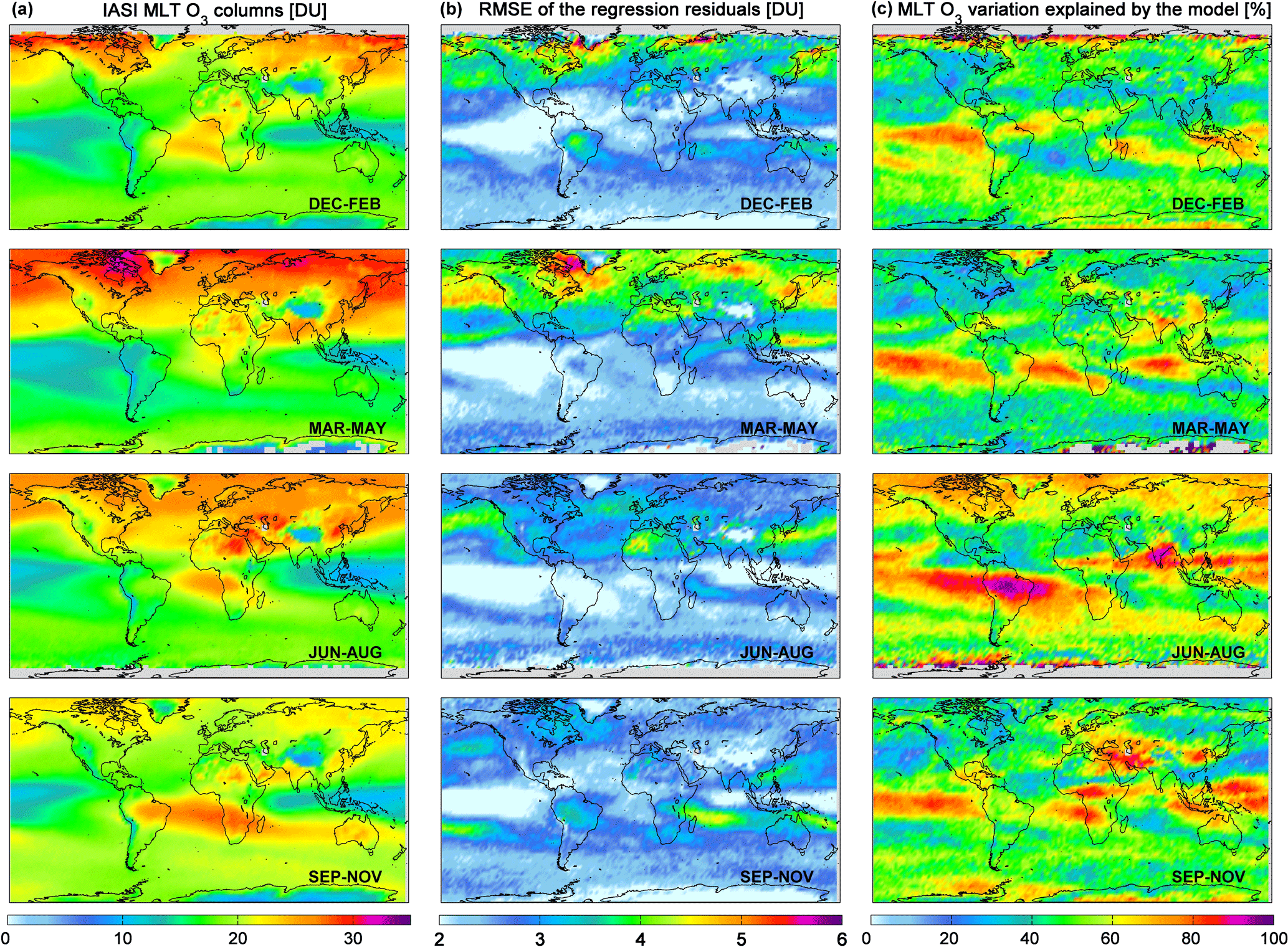
Figure 1 Seasonal distribution of O₃ tropospheric columns (in DU, integrated from ground to 300 hPa) measured by IASI and averaged over January 2008–May 2017 (a), of the RMSE of the regression fits (in DU, b) and of the fraction of the variation in IASI data explained by the regression model, calculated as $\mathrm{100}\times \left(\mathit{\sigma }\left({{\mathit{O}}_{\mathbf{3}}}^{\text{Fitted\_ model}}\left(t\right)\right)/\mathit{\sigma }\left({\mathit{O}}_{\mathbf{3}}\left(t\right)\right)\right)$ (in percent, c). Data are averaged over a 2.5^∘ × 2.5^∘ grid box.

3 Regression performance and sensitivity to trend

In this section, we first verify the performance of the MLR models (annual and seasonal; in terms of residual errors and variation explained by the model) to globally reproduce the time evolution of O₃ records over the entire studied period (January 2008–May 2017). Based on this, we then investigate the statistical relevance of a trend study from IASI measurements in the troposphere by examining the sensitivity of the pair IASI-MLR to the retrieved LT term.

Figure 1 presents the seasonal distributions of tropospheric O₃ measured by IASI averaged over January 2008–May 2017 (Fig. 1a), along with the RMSE of the seasonal regression fit (in DU; Fig. 1b) and the contribution of the fitted seasonal model into the IASI O₃ time series (in percent; Fig. 1c), calculated as $\frac{\mathit{\sigma }\left({{\mathit{O}}_{\mathbf{3}}}^{\mathrm{Fitted}\mathrm{\_}\mathrm{model}}\left(t\right)\right)}{\mathit{\sigma }\left({\mathit{O}}_{\mathbf{3}}\left(t\right)\right)}$, where σ is the standard deviation relative to the regression models and to the IASI O₃ time series. These two statistical parameters help to evaluate how well the fitted model explains the variability in the IASI O₃ observations. The seasonal patterns of O₃ measurements are close to those reported in Wespes et al. (2017) for a shorter period (see Sects. 2.1 and 3.1 in Wespes et al., 2017 for a detailed description of the distributions) and they clearly show, for instance, high O₃ values over the highly populated areas of Asia in summer. The distributions from Fig. 1 show that the model reproduces between 35 and 90 % of the daily O₃ variation captured by IASI and that the residual errors vary between 0.01 and 5 DU (i.e., the RMSEs relative to the IASI O₃ time series are of ∼ 15 % on global average and vary between 10 % in the NH in summer and 30 % in specific tropical regions). On an annual basis (data not shown), the model explains a large fraction of the variation in the IASI O₃ dataset (from ∼ 45 to ∼ 85 %) and the RMSEs are lower than 4.5 DU everywhere (∼ 3 DU on the global average). The relative RMSE is less than 1 % in almost all situations indicating the absence of bias.

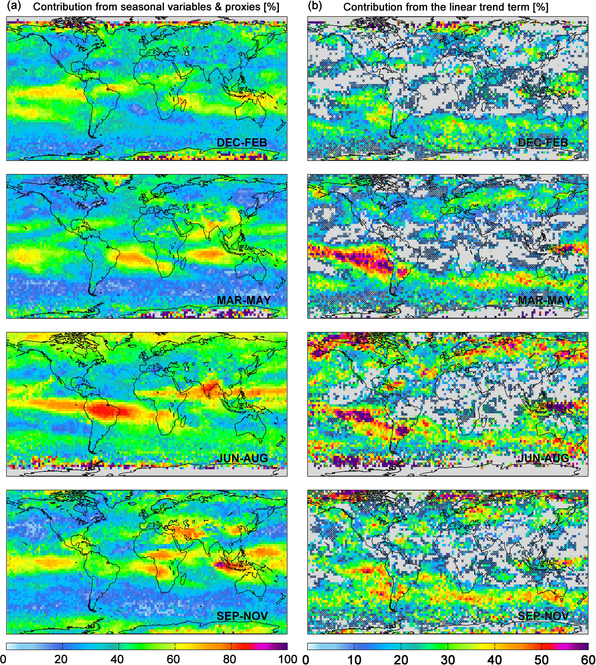
Figure 2 Seasonal distributions of the contribution from the seasonal and explanatory variables into the IASI O₃ variations estimated as $\left[\mathrm{100}\times \mathit{\sigma }\left(\sum _{n=\mathrm{1};j=\mathrm{2}}^{\mathrm{4};m}\left[a_n;b_n;x_j\right]\left[\cos \left(n\mathit{\omega }t\right);\sin \left(n\mathit{\omega }t\right);{\mathit{X}}_{\mathrm{norm},\mathit{j}}\left(t\right)\right]\right)/\mathit{\sigma }\left({\mathit{O}}_{\mathbf{3}}\left(t\right)\right)\right]$ (in percent, a) and of the contribution from the linear trend calculated as $\left[\mathrm{100}\times \mathit{\sigma }\left(x_{j=\mathrm{1}}\cdot \mathit{\text{trend}}\right)/\mathit{\sigma }\left({\mathit{O}}_{\mathbf{3}}\left(t\right)\right)\right]$ (in percent, b). The grey areas and crosses refer to the non-significant grid cells in the 95 % confidence limits (2σ level). Note that the scales are different.

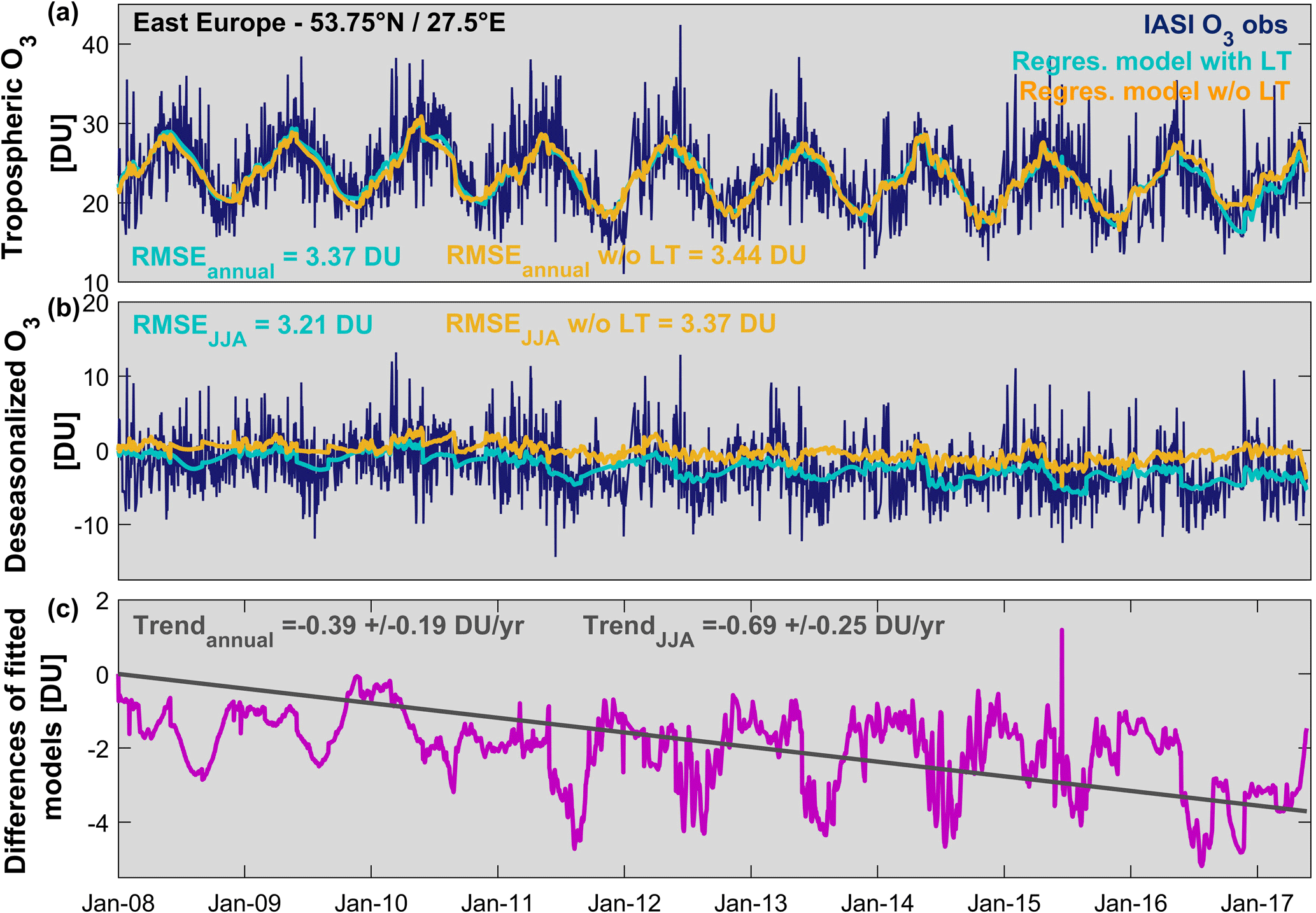
Figure 3 (a) Example of daily time series of IASI O₃ measurements (dark blue) and of the fitted seasonal regression models with (light blue) and without (orange) the linear term in the troposphere. Daily time series (b) of the deseasonalized O₃ (observations and regression models) and (c) of the difference of the fitted models with and without the linear trend term as well as the adjusted annual trend (pink and grey lines, respectively; c; given in DU). The RMSE (annual and for the JJA period in DU) and the trend values (annual and for the JJA period in DU yr⁻¹) are also indicated.

The seasonal distributions of the contribution to the total variation in the MLT from the adjusted harmonic terms and explanatory variables, which account for the “natural” variability, and from the LT term are shown in Fig. 2a and b, respectively. The grey areas in the LT panels refer to the LT terms rejected by the stepwise backward elimination process. The crosses indicate that the trend estimate in the grid cell is non-significant at the 95 % confidence limits (2σ level) when accounting for the autocorrelation in the noise residual at the end of the elimination procedure. While the large influences of the seasonal variations and of the main drivers – namely ENSO, NAO and QBO – on the IASI O₃ records have been clearly attested in Wespes et al. (2017), we demonstrate in Fig. 2 that the LT also contributes considerably to the O₃ variations detected by IASI in the troposphere. The LT contribution generally ranges from 15 to 50 %, with the largest values (∼ 30 to ∼ 50 %) being observed at mid- and high latitudes in the SH (30–70^∘ S) and in the NH (45–70^∘ N) in summer. In the SH, they are associated with the smallest tropospheric O₃ columns (Fig. 1a) and the smallest natural contributions (< 25 %; Fig. 2a), while in the NH summer, they interestingly correspond to large MLT O₃ columns, large natural contributions (∼ 50 to ∼ 60 %) and the smallest RMSE (< 12 % or < 3 DU). From the annual regression model, the natural variation and the trend respectively contribute 30–85 % and up to 40 % to the total variation in the MLT.

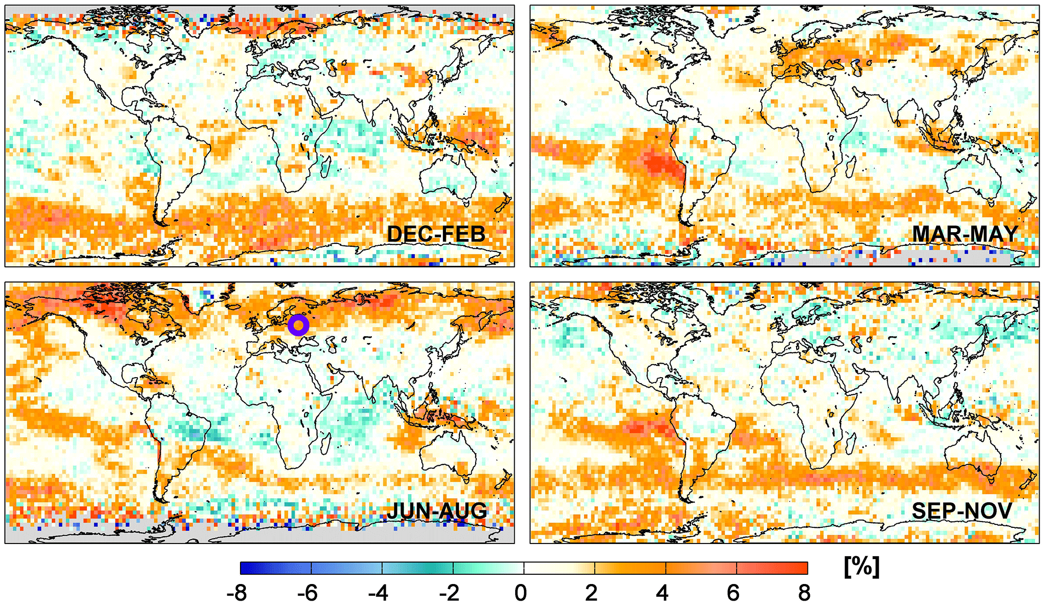
Figure 4 Seasonal distribution of the differences between the RMSE of the regression fits with and without the linear trend term [(RMSE_{_w/o_LT} − RMSE_{_with_LT}) ∕ RMSE_{_with_LT}×100] (in percent). The blue circle in the JJA panel refers to the case presented in Fig. 3.

In Fig. 3, we further investigate the robustness of the estimated trends by performing sensitivity tests in regions of significant trend contributions (e.g., in the NH midlatitudes in summer; see Fig. 2). The ∼ 9-year time series of IASI O₃ daily averages (dark blue) along with the results from the seasonal regression model with and without the LT term included in the model (light blue and orange lines, respectively) are represented in Fig. 3a for one specific location (highlighted by a blue circle in the JJA panel in Fig. 4). Figure 3b provides the deseasonalized IASI (dark blue line) and fitted time series (calculated by subtracting the adjusted seasonal cycle from the time series) resulting from the adjustment with and without the LT term included in the MLR model (light blue and orange lines, respectively). The differences between the fitted models with and without LT are shown in Fig. 3c (pink lines). They match fairly well the adjusted trend over the IASI period (Fig. 3c, grey lines; the trend and the RMSE values are also indicated) and the adjustment without LT leads to larger residuals (e.g., RMSE_{_JJA_w/o_LT}=3.37 DU vs. RMSE_{_JJA_with_LT}=3.21 DU in summer). This result demonstrates the possibility of capturing trend information from ∼ 9 years of IASI-MLR with only some compensation effects from the other explanatory variables, contrary to what was observed when considering a shorter period of measurements or less-frequent sampling (i.e., monthly dataset; e.g., Wespes et al., 2016). It is also worth mentioning that the O₃ change calculated over the whole IASI dataset in summer is larger than the RMSE of the model residuals (increase of 6.50 ± 2.35 DU vs. RMSE of 3.21 DU), underlying the statistical relevance of trend estimates.

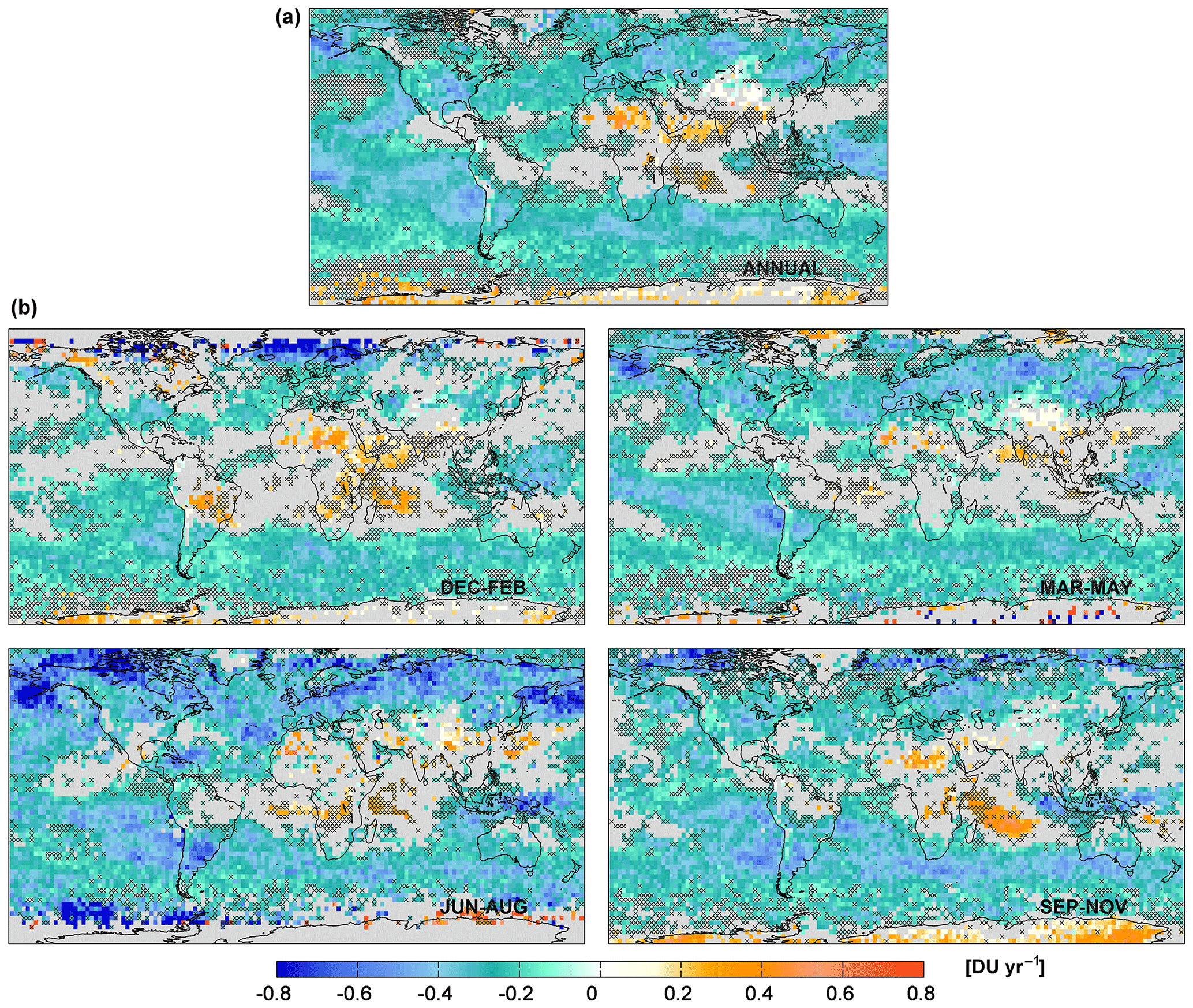
Figure 5 (a) Annual and (b) seasonal distributions of the adjusted trends in DU yr⁻¹ from the multi-linear regression models. The grey areas and crosses refer to the non-significant grid cells in the 95 % confidence limits (2σ level).

The robustness of the adjusted trend is verified at the global scale in Fig. 4 which represents the seasonal distributions of the relative differences in the RMSE with and without the LT included in the MLR model, calculated as (RMSE_{_w/o_LT} − RMSE_{_with_LT}) ∕ RMSE_{_with_LT}×100 (in percent). An increase in the RMSE when excluding LT from the MLR is observed almost everywhere in regions of significant trend contributions (Fig. 2), especially in mid- and high latitudes of the SH and of the NH in summer, where it reaches 10 %. This result indicates that adjusting LT improves the performance of the model and, hence, that a trend signal is well captured by IASI at a regional scale in the troposphere. From the annual model, the increase in the RMSE only reaches 5 % at mid- and high latitudes of the SH (data not shown). In regions of weak or non-significant trend contribution (see crosses in Fig. 2), no improvement is logically found.

4 O₃ trend over 2008–2017

4.1 Annual and seasonal trends

The annual and the seasonal distributions of the fitted LT terms which are retained in the annual and the seasonal MLR models by the stepwise elimination procedure are respectively represented in Fig. 5a and b (in DU yr⁻¹). Generally, the mid- and high latitudes of both hemispheres and, more particularly, the NH midlatitudes in summer reveal significant negative trends, while the tropics are mainly characterized by non-significant or weak significant trends. Even if trends in emissions have already been able to qualitatively explain measured tropospheric O₃ trends over specific regions, the magnitude and the trend estimates considerably vary between independent measurement datasets (e.g., Cooper et al., 2014; the TOAR-Climate report coordinated by the International Global Atmospheric Chemistry Project and available soon at http://www.igacproject.org/activities/TOAR, last access: 8 May 2018, of Gaudel et al., 2018, and references therein) for the reasons discussed in Sect. 1, and they are not reproduced/explained by model simulations (e.g., Jonson et al., 2006; Cooper et al., 2010; Logan et al., 2012; Wilson et al., 2012; Hess and Zbinden, 2013; and references therein). As a result, comparing/reconciling the adjusted trends with independent measurements, even on a qualitative basis, remains difficult. Nevertheless, several of the statistically significant features observed in Fig. 5 show, interestingly, qualitative consistency with respect to recent published findings:

• The SH tropical region extending from the Amazon to tropical eastern Indian Ocean seems to indicate a general increase with, for example, a DJF trend of ∼ 0.23 ± 0.18 DU yr⁻¹ (i.e., 2.09 ± 1.70 DU over the IASI measurement period), despite the large IAV in the MLT which characterizes the tropics and which likely explains the high frequency of non-significant trends. Enhanced O₃ levels over that region have already been analyzed for previous periods (e.g., Logan, 1985; Logan and Kirchhoff, 1986; Fishman et al., 1991; Moxim and Levy, 2000; Thompson and Wallace, 2000; Thompson et al., 2007; Sauvage et al., 2006, 2007; Heue et al., 2016; Ebojie et al., 2016; Archibald et al., 2018; Leventidou et al., 2017). For instance, the large O₃ enhancement of ∼ 0.36 ± 0.25 DU yr⁻¹ (i.e., 3.3 ± 2.3 DU over the whole IASI period) stretching from southern Africa to Australia over the northeast of Madagascar during the austral winter–spring likely originates from large IAV in the subtropical jet-related stratosphere–troposphere exchanges, which have been found to primarily contribute to the tropospheric O₃ trends over that region (Liu et al., 2016, 2017). Nevertheless, this finding should be mitigated by the fact that the trend value in the SH tropics is of the same magnitude as the RMSE of the regression residuals (∼ 2 to ∼ 4.5 DU; see Fig. 1).

  Conversely, the tropical Pacific region exhibits significant negative trends that are similar to those reported from UV sounders in Ebojie et al. (2016) and in Leventidou et al. (2017) over previous periods, while Heue et al. (2016) mainly report a significant positive trend over that region.

• The trends over Southeast Asia are mostly non-significant and vary by season. In spring–summer, some grid cells in India, in mainland China and eastern downwind China exhibit significant positive trends reaching ∼ 0.45 DU yr⁻¹ (i.e., ∼ 4.2 DU over the IASI measurement period). This tends to indicate that the tropospheric O₃ increases, which have been shown to mainly result from a strong positive trend in the Asian emissions over the past decades (e.g., Zhao et al., 2013; Cooper et al., 2014; Zhang et al., 2016; Cohen et al., 2017; Tarasick et al., 2018; and references therein) but also from a substantial change in the stratospheric contribution (Verstraeten et al., 2015), persist through 2008–2017 despite the recent decrease in O₃ precursor emissions recorded in China after 2011 (e.g., Duncan et al., 2016; Krotkov et al., 2016; Miyazaki et al., 2017; van der A et al., 2017). This would indicate that this decrease is probably too recent/weak to recover the 2008 O₃ levels over the entire region. Significant positive trends over Southeast Asia have also been reported from UV sounders over previous periods (e.g., Ebojie et al., 2016). Note, however, that this finding has to be taken carefully given the large model residuals (RMSE of ∼ 2 to ∼ 4 DU; see Sect. 3, Fig. 1) over that region. Finally, the large uncertainty in trend estimates over Southeast Asia might reflect the large IAV in the biomass-burning emissions and lightning NO_x sources, in addition to the recent changes in emissions.

• The mid- and high latitudes of the SH show clear patterns of negative trends, throughout the year and in a more pronounced manner during winter–spring, with larger amplitudes than those of the RMSE values (∼ −0.33 ± 0.14 DU yr⁻¹ on average in the 35–65^∘ S band; i.e., a trend amplitude of ∼ $\left|\mathrm{3.1}\right|$ ± 1.3 DU over the studied period vs. an RMSE value of ∼ 2.5 DU). These significant negative trends in the SH are hard to explain, but considering the stratospheric contribution into the tropospheric columns (natural and artificial due to the limited IASI vertical sensitivity) in the mid- and high latitudes of the SH (∼ 40 to ∼ 60 %; see Supplement in Wespes et al., 2016) and the negative significant trends previously reported from IASI in the UTLS/low stratosphere in the 30–50^∘ S band, they could be in line with those derived by Zeng et al. (2017) in the UTLS for a clean rural site of the SH (Lauder, New Zealand), which mainly originate from increasing tropopause height and O₃-depleting substances. Significant negative change in tropospheric O₃ over these regions were also reported in Ebojie et al. (2016).

• In the NH, a band-like pattern of negative trends is observed in the 40–75^∘ N band covering Europe and North America, especially during summer. Averaged annual trend of −0.31 ± 0.17 DU yr⁻¹ and summer trend of −0.47 ± 0.22 DU yr⁻¹ (i.e., −2.87 ± 1.57 and −4.36 ± 2.02 DU, respectively, from January 2008 to May 2017) are estimated in that latitudinal band. These trend values are significantly larger than the RMSEs of the MLR model (< 3.5 DU in JJA; see Sect. 3, Fig. 1). Interestingly, both the annual and summer trends are amplified relative to the ones calculated in the midlatitudes of the NH over the 2008–2013 period of IASI measurements (−0.19 ± 0.05 DU yr⁻¹ and −0.30 ± 0.10 DU yr⁻¹ for the annual and the summer trends, respectively, calculated in the 30–50^∘ N band; see Wespes et al., 2016). This finding is line with previous studies which point out a possible leveling off of tropospheric O₃ in summer due to the decline of anthropogenic O₃ precursor emissions observed since 2010-2011 in North America, in western Europe and also in some regions of China (e.g., Cooper et al., 2010, 2012; Logan et al., 2012; Parrish et al., 2012; Oltmans et al., 2013; Simon et al., 2015; Ebojie et al., 2016; Archibald et al., 2018; Miyazaki et al., 2017). The present study even goes a step further by suggesting a possible decrease in the tropospheric O₃ levels. Archibald et al. (2018) recently reported a net decrease of ∼ 5 % in the global anthropogenic NO_x emissions in the 30–90^∘ N latitude band, which is consistent with the annual significant negative trend of −0.27 ± 0.15 DU yr⁻¹ for O₃ estimated from IASI in that band. We should also note that, even if these latitudes are characterized by the lowest stratospheric contribution (∼ 30 to ∼ 45 %; see Supplement in Wespes et al., 2016), it might partly mask/attenuate the variability in the tropospheric O₃ levels.

4.2 Expected year for trend detection

In this section, we further verify that it is indeed possible to infer, from the studied IASI period, the significant negative trend derived in the 40–75^∘ N band in summer (∼ $\left|\mathrm{0.5}\right|$ DU yr⁻¹ on average; see Sect. 4.1) by determining the expected year from which such a trend amplitude would be detectable at a global scale. This is achieved by estimating the minimum duration (with probability 0.90) of the IASI O₃ measurements that would be required to detect a trend of a specified magnitude, and its 95 % confidence level, following the formalism developed in Tiao et al. (1990) and in Weatherhead et al. (1998):

$$\begin{array}{}\text{(1)}& {\displaystyle }& {\displaystyle }{N}^{\ast }\approx {\left[{\displaystyle \frac{\mathrm{3.3}\cdot {\mathit{\sigma }}_{\mathit{\epsilon }}}{\left|{\mathit{\tau }}_{\mathrm{yr}}\right|}}\cdot \sqrt{{\displaystyle \frac{\mathrm{1}+\mathit{\varphi }}{\mathrm{1}-\mathit{\varphi }}}}\right]}^{\frac{\mathrm{2}}{\mathrm{3}}},\text{(2)}& {\displaystyle }& {\displaystyle }{\mathrm{CL}}_{N^{\ast }}=\left[N^{\ast }\cdot e^{-B};N^{\ast }\cdot e^{+B},\right]\end{array}$$

where N^∗is the number of the required years, σ_ε is the standard deviation of the autoregressive noise residual ε_t, τ_yr is the magnitude of the trend per year and ϕ is the lag-1 autocorrelation of the noise. The magnitudes of the variation and the autocorrelation in the noise residuals are taken into account for reaching a better trend estimate precision. Given that large variance (${\mathit{\sigma }}_{\mathit{\epsilon }}^{\mathrm{2}})$ and large positive autocorrelation ϕ of the noise induce small signal-to-noise ratio and long trend-like segments in the dataset, respectively, these two parameters increase the number of years that would be required for detecting a specified trend. CL${}_{N^{\ast }}$ is the 95 % confidence limit, which is not symmetric around N^∗and depends on B, an estimated uncertainty factor calculated as $\frac{\mathrm{4}}{\mathrm{3}\sqrt{D}}\sqrt{\frac{\mathrm{1}+\mathit{\varphi }}{\mathrm{1}-\mathit{\varphi }}}$, with D the number of days in the IASI datasets, which accounts for the uncertainty in ϕ (the uncertainty in σ_ε being negligible given that only a few years of data are needed to estimate it; see Weatherhead et al., 1998). As a result, based on the available IASI-A and proxies datasets and assuming that the MLR model used in this study is accurate, we estimate, in Fig. 6a and b, the expected year when an O₃ trend amplitude of $\left|\mathrm{5}\right|$ DU decade⁻¹ (i.e., ${\mathit{\tau }}_{\mathrm{yr}}=\left|\mathrm{0.5}\right|$ DU yr⁻¹ which corresponds to the averaged absolute value of the fitted negative trends in the NH summer; see Fig. 5b) is detectable, and its associated maximal confidence limit, respectively. The results in Fig. 6 clearly demonstrate the possibility of inferring, from the available IASI dataset, such significant trends in the mid- and high latitudes of the NH in summer and fall (trend detectable from ∼ 2016 to 2017 with an uncertainty of ∼ 6 to ∼ 9 months; see Fig. 6b). Conversely, the tropical regions and the NH in winter–spring would require additional ∼ 6 months to ∼ 6 years of measurements to detect an amplitude of $\left|\mathrm{0.5}\right|$ DU yr⁻¹ (trend significant only from ∼ 2017 to 2023 or after depending on the location and the season). Note also that the strongest negative trends (up to −0.85 DU yr⁻¹, i.e., ${\mathit{\tau }}_{\mathrm{yr}}=\left|\mathrm{0.85}\right|$ DU yr⁻¹; see Fig. 5b) observed in specific regions of the NH midlatitudes would only require ∼ 6 years of IASI measurements for being detected. The mid- and high latitudes of the SH would require the shortest period of IASI measurement for detecting a specified trend, with only ∼ 7 years ± ∼ 6 months of IASI measurements to detect a $\left|\mathrm{0.5}\right|$ DU yr⁻¹ trend (trend detectable from ∼ 2015). That band-like pattern in the SH corresponds to the region with the weakest IAV and contribution from large-scale dynamical modes of variability in the IASI MLT columns (see Sect. 3, Figs. 1 and 2), which translates into small ${\mathit{\sigma }}_{\mathit{\epsilon }}^{\mathrm{2}}$ and ϕ. Note however that an additional few months of IASI data are required to confirm the smaller negative trend of ∼ −0.35 DU yr⁻¹ measured on average in the SH (see Fig. 5; a period ∼ 9 years ± ∼ 6 months being necessary to detect a trend amplitude of $\left|\mathrm{3.5}\right|$ DU decade⁻¹). Given that large σ_ε means large noise residual in the IASI data, the regions of short (long) required measurement period coincide, as expected, well with the small (high) RMSE values of the regression residuals (see Sect. 3, Fig. 1).

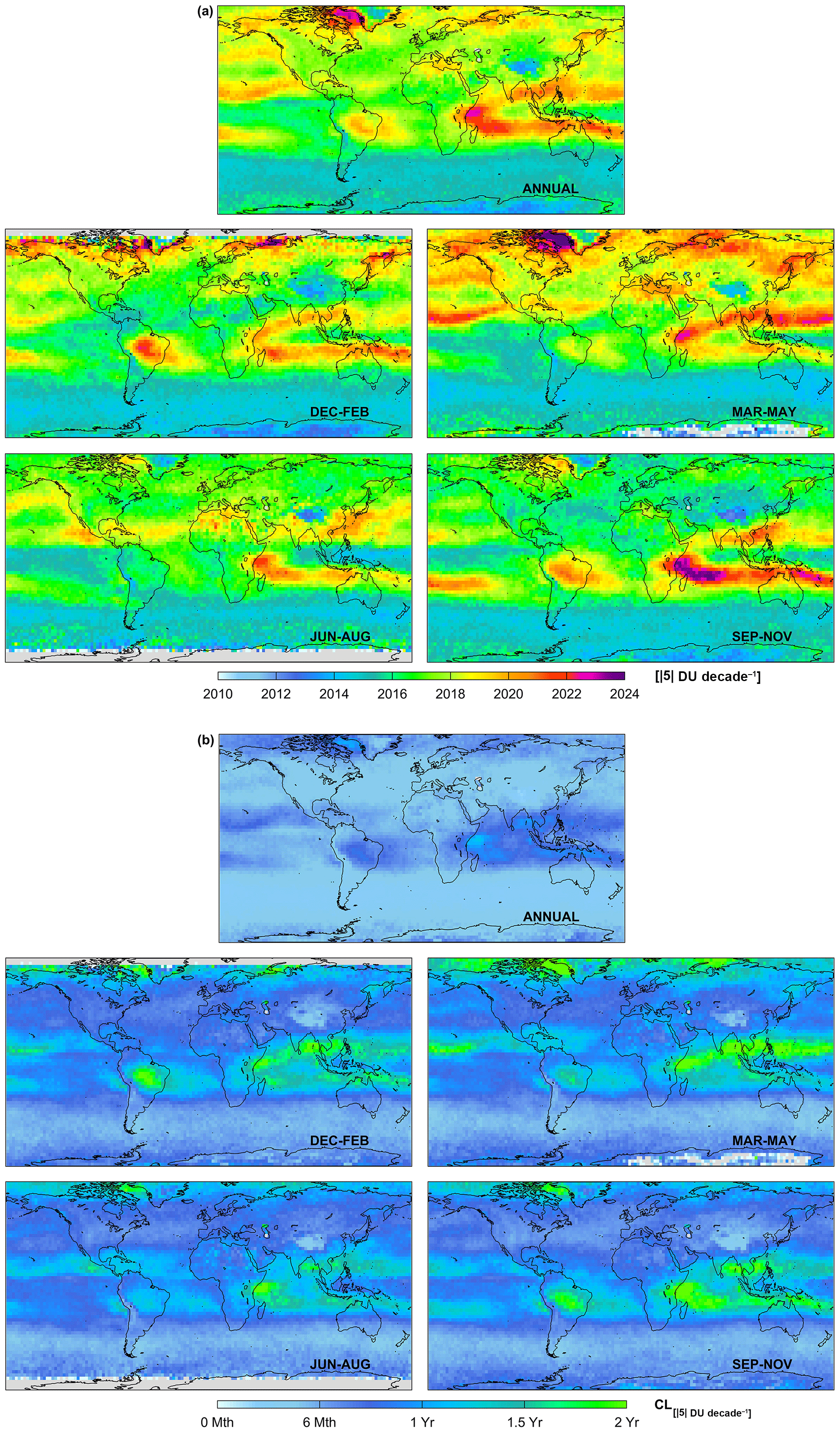
Figure 6 (a) Estimated year of tropospheric IASI O₃ trend detection (with a probability of 90 %) for a given trend of $\left|\mathrm{5}\right|$ DU decade⁻¹ starting at the beginning of the studied period (20080101) and (b) associated maximal confidence limits from the annual (top panel) and the seasonal (bottom panels) regression models.

The regions of the longest measurement periods required in the tropics for the $\left|\mathrm{5}\right|$ DU decade⁻¹ trend detection (up to ∼ 16 years of IASI data) correspond to known patterns of widespread high O₃: (a) above intense biomass burning in Amazonia and eastwards across the tropical Atlantic (Logan and Kirchhoff, 1986; Fishman et al., 1991; Moxim and Levy, 2000; Thompson and Wallace, 2000; Thompson et al., 2007; Sauvage et al., 2007), (b) eastwards of Africa across the southern Indian Ocean which is subject to large variations in the stratospheric influences during the winter–spring austral period (JJA–SON; Liu et al., 2016, 2017), (c) eastwards of Africa across the northern Indian Ocean to India likely due to large lightning NO_x emissions above central Africa during the wet season associated with the northeastward jet conducting a so-called “O₃ river” (Tocquer et al., 2015) and (d) above regions of positive ENSO “chemical” effect in equatorial Asia/Australia and eastwards above northern and southern tropical regions (Wespes et al., 2016) explained by reduced rainfall and biomass fires during El Niño conditions (e.g., Worden et al., 2013). In fact, most of these patterns (a, b and d) are closely connected with strong El Niño events which extend the duration of the dry season and cause severe droughts, producing intense biomass-burning emissions, for instance, over South America (e.g., Chen et al., 2011; Lewis et al., 2011) and South Asia/Australia (e.g., Oman et al., 2013; Valks et al., 2014; Ziemke et al., 2015), and which alter the tropospheric circulation by increasing the transport of stratospheric O₃ into the troposphere (e.g., Voulgarakis et al., 2011b; Neu et al., 2014) and the transport of biomass-burning air masses to the Indian Ocean (Zhang et al., 2012). In summary, these large-scale indirect ENSO-related variations in tropospheric O₃ and the lightning NO_x impact on O₃, which are not accounted for in the MLR by specific representative proxies, are misrepresented in the regression models. They induce large noise residuals, i.e., large σ_ε, and hence extend the time period needed to detect a trend of any given magnitude.

Figure 6, finally, suggests that a long duration is also required, especially in summer, above and east of China to quantify the anthropogenic impact on the local changes in the MLT: additional 3 ± 1.5 or 5 ± 1.5 years for a given $\left|\mathrm{5}\right|$ or $\left|\mathrm{3.5}\right|$ DU decade⁻¹ trend are respectively calculated. This result could be explained by large perturbations in the MLT columns induced by recent decreases after decades of almost constant increases in surface emissions in China (e.g., Cohen et al., 2017; Miyazaki et al., 2017).

4.3 Multi-linear vs. single linear model

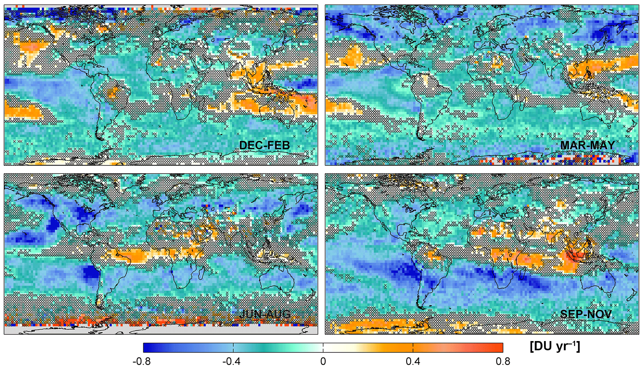
Figure 7 Seasonal distributions of the fitted linear term trends (given in DU yr⁻¹) derived from a single linear regression model. The crosses refer to the non-significant grid cells in the 95 % confidence limits (2σ level).

Even if MLR models have already been used for extracting trends in stratospheric and total O₃ columns (e.g., Mäder et al., 2007; Frossard et al., 2013; Rieder et al., 2013; Knibbe et al., 2014), single linear regression (SLR) models, which do not differentiate the natural (chemical and dynamical) factors describing the O₃ variability, are still commonly used (e.g., Cooper et al., 2014; the TOAR-Climate report of Gaudel et al., 2018; and references therein). They are, however, suspected to contribute to trend biases retrieved between independent measurements. In addition to the time-varying instrumental biases, trend biases can also be related to differences in the spatial and the temporal samplings (e.g., Doughty et al., 2011; Saunois et al., 2012; Lin et al., 2015), in the measurement period, in the upper boundary of the O₃ columns, in the algorithm and in the vertical sensitivity of the measurements. The latter artificially alters the characteristics of the sounded layer by contaminations from the above and below layers leading to a mixing of the trend and also of the natural characteristics originating from these different layers (e.g., troposphere and stratosphere). The differences in the studied period, in the tropopause definition and in the spatio-temporal sampling might also imply differences in the natural influence on the measured O₃ variations. While the impact of the natural contribution is taken into account in the MLR model, it might introduce an additional bias in the trend determined from SLR, making further challenging to compare trends estimated from a series of inhomogeneous independent measurements.

Substantial efforts in homogenizing independent tropospheric O₃ column (TOC) datasets have been made in the TOAR-Climate assessment report (Gaudel et al., 2018), but large SLR trend biases remain between the TOAR datasets, in particular, between the satellite datasets where the lack of homogeneity in terms of tropopause calculation (same tropopause definition but different temperature profiles are used), of instrument vertical sensitivities and of spatial sampling have been specifically raised as possible causes for the trend divergence.

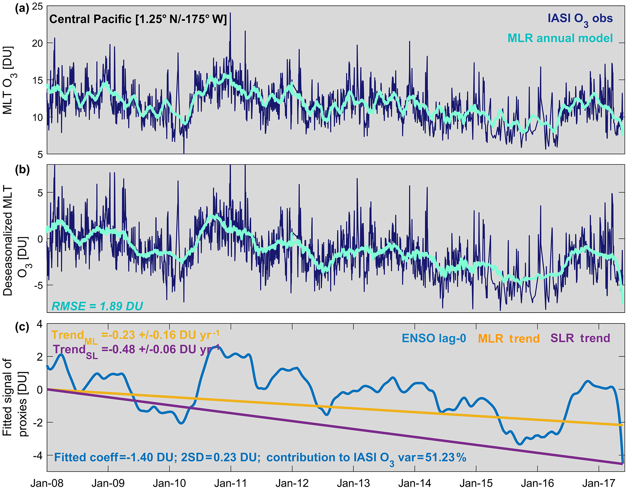
Figure 8 Daily time series of (a) O₃ measured by IASI (dark blue) and adjusted by the multivariate annual regression model (light blue), (b) the deseasonalized O₃ and (c) the fitted signal of ENSO proxy (one of the main retained proxies in the multivariate regression model) calculated as x_jX_norm,j (given in DU) along with the adjusted trends derived from the single and the multivariate linear regressions (SLR and MLR) over the equatorial central Pacific (region of negative ENSO “dynamical” effect). The RMSE of the MLR fit and the fitted SLR and MLR trend values are also indicated.

If reconciling the trend biases between the datasets by applying the vertical sensitivity of each measurement type to a common platform, as proposed in the TOAR-Climate assessment report is beyond the scope of this study and if, at this stage, there is no consensus in determining tropospheric O₃ trends, the improvement in using a MLR instead of a SLR model for determining more accurate/realistic trends is explored here by comparing the seasonal distributions of the trends estimated from MLR (see Fig. 5b in Sect. 4.1.) and from SLR (presented in Fig. 7). Note that the constant term in the SLR model is split into two components (covering the periods before and after the September 2010 jump) to take account of the observed jump (see Sect. 2). The highest differences in the fitted trends derived from the two methods are found in the tropics and in some regions of the midlatitudes of the NH. They likely result from overlaps between the LT term and other covariates. For instance, the regions with high significant SLR trends (∼ 0.3 to ∼ 0.6 DU yr⁻¹ over the tropical western and middle Pacific) during the period extending from September to May match the regions with strong El Niño/Southern Oscillation influence (see Figs. 8 and 12 in Wespes et al., 2016). Conversely, the MLR model shows generally weak significant negative or non-significant trends in the Pacific El Niño region during that period and it would even need additional ∼ 3 to ∼ 4 years of IASI measurements for detecting the fitted SLR trends (see Sect. 4.2 above). The effect of ENSO in overestimating the fitted SLR trend is further illustrated in Fig. 8 which represents the time series of O₃ observed by IASI and adjusted by the annual MLR model (Fig. 8a) along with the deseasonalized times series (Fig. 8b) and the fitted SLR and MLR trends (Fig. 8c). The fitted signal of the ENSO proxy from the MLR model (calculated as x_jX_norm,j following Wespes et al., 2017) is also represented (Fig. 8c). That example clearly shows that the ENSO influence is considerably compensated for by the adjustment of the linear trend in the SLR (annual trend of −0.48 ± 0.06 DU yr⁻¹ from SLR vs. −0.23 ± 0.16 DU yr⁻¹ from MLR for that example). Finally, differences between the SLR and the MLR models are also observed in the region with strong positive NAO influence over the Icelandic/Arctic region during MAM (see Wespes et al., 2016, for a description of the NAO-related O₃ changes). Conversely, the sub-tropical SH exhibits similar seasonal patterns of negative trends from both the SLR and the MLR. This results from the weak natural IAV and contributions in tropospheric O₃ above that region (see Sect. 3, Figs. 1 and 2), which, hence, limits the compensation effects.

In summary, despite the fact that considering a long period of measurements is usually recommended in SLR studies to overcome the dynamical cycles and, hence, to help in differentiating their influences from trends, we show that, considering that some dynamics have irregular or no particular periodicity (e.g., NAO, ENSO), it is not accurate enough. Furthermore, accurate satellite measurements of tropospheric O₃ at a global scale are quite recent, limiting the period of available and comparable datasets (e.g., Payne et al., 2017). As a consequence, we support here that using a reliable multivariate regression model based on geophysical parameters and adapted for each specific sounded layer is a robust method for differentiating a “true” trend from any other sources of variability and, hence, that it should help in resolving trend differences between independent datasets.

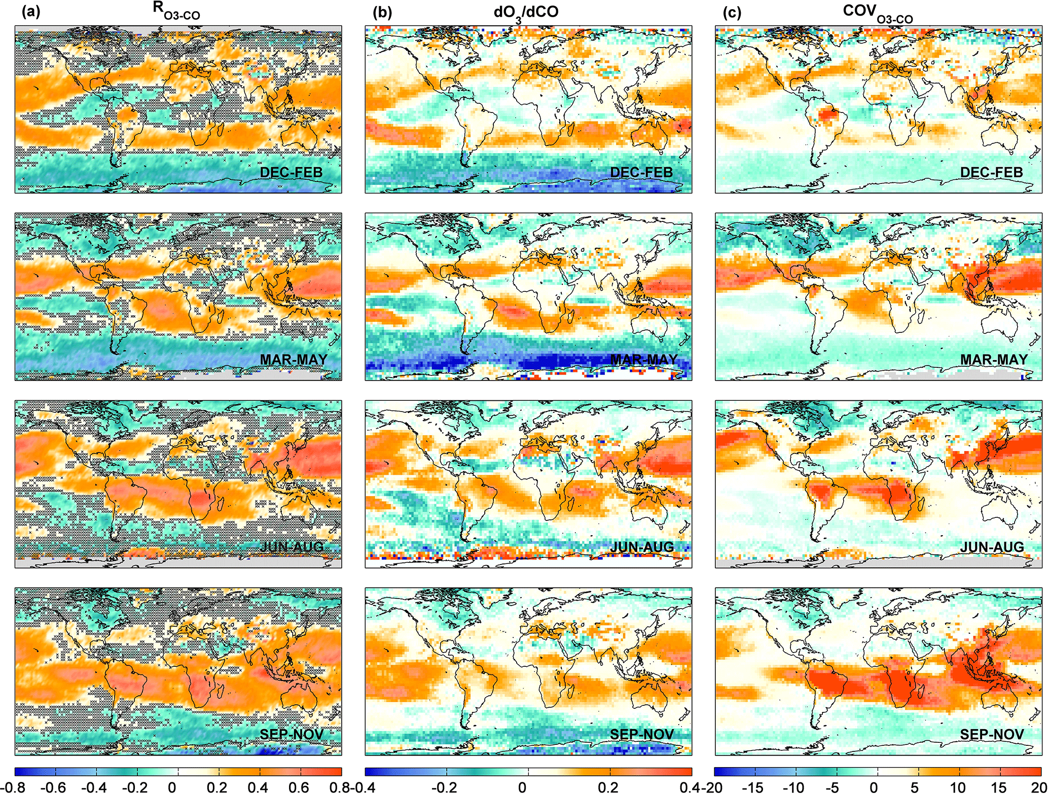
Figure 9 Global distributions of (a) the correlation coefficients ($R_{{\mathrm{O}}_{\mathrm{3}}-\mathrm{CO}})$, (b) the regression slope (dO₃ ∕ dCO in mol cm⁻²/mol cm⁻²) and (c) the covariances (COV${}_{{\mathrm{O}}_{\mathrm{3}}-\mathrm{CO}}$ in 10³³ mol cm⁻² × mol cm⁻²) of daily median IASI tropospheric O₃ and CO over January 2008–May 2017. Data are averaged over a 2.5^∘ × 2.5^∘ grid box. Crosses in $R_{{\mathrm{O}}_{\mathrm{3}}-\mathrm{CO}}$ (a) refer to the non-significant grid cells in the 95 % confidence intervals (2σ level).

4.4 Continental influence

In this section, we use the capabilities of IASI to simultaneously measure O₃ and CO in order (1) to differentiate tropospheric and stratospheric air masses, (2) to identify the regions influenced by the continental export/intercontinental transport of O₃ pollution and (3) to evaluate that continental influence on tropospheric O₃ trends as observed by IASI. Similar tracer correlations between CO and O₃ have already been used to give insights into the photochemical O₃ enhancement in air pollution transport (e.g., Parrish et al., 1993; Bertschi and Jaffe, 2005). However, there are only a few studies using global satellite data for this purpose (Zhang et al., 2006; Voulgarakis et al., 2011a; Kim et al., 2013) and the analysis of the O₃–CO relationship for better understanding the origin of O₃ trends in the troposphere has, to the best of our knowledge, never been explored.

Figure 9a and b show the seasonal patterns of the O₃–CO correlations (referred as $R_{{\mathrm{O}}_{\mathrm{3}}-\mathrm{CO}})$ and of the dO₃ ∕ dCO regression slopes calculated in the troposphere (from the surface to 300 hPa) over the studied IASI period (January 2008–May 2017). The dO₃ ∕ dCO regression slopes, which represent the so-called O₃–CO enhancement ratio, are used to evaluate the photochemical O₃ production in continental outflow regions. The $R_{{\mathrm{O}}_{\mathrm{3}}-\mathrm{CO}}$ and the dO₃ ∕ dCO distributions are similar and clearly show regional and seasonal differences in the strength of the O₃–CO relationships. The patterns of positive and negative correlations allows differentiating the outflow regions characterized by photochemical O₃ production from precursors (including CO) or CO destruction (both identified by positive $R_{{\mathrm{O}}_{\mathrm{3}}-\mathrm{CO}})$ from the regions characterized by O₃ loss (chemical destruction or surface deposition) or by strong stratospheric contaminations (both identified by negative $R_{{\mathrm{O}}_{\mathrm{3}}-\mathrm{CO}})$. Negative $R_{{\mathrm{O}}_{\mathrm{3}}-\mathrm{CO}}$ and dO₃ ∕ dCO are measured at high latitudes of both hemispheres all over the year, but more specifically at high latitudes of the SH in summer–fall (with $R_{{\mathrm{O}}_{\mathrm{3}}-\mathrm{CO}}$ < −0.25 on averages in DJF and MAM). Given that high latitudes experience more O₃ destruction than the low latitudes due to a lack of sunlight, the negative correlations for the high latitude regions might also reflect air masses originating from/characterizing the stratosphere due to natural intrusion or to artificial mixing with the troposphere introduced by the limited vertical sensitivity of IASI in the highest latitudes (stratospheric contribution varying between ∼ 40 and ∼ 65 %; see Supplement in Wespes et al., 2016). These processes are likely at the origin of the band-like pattern of negative trends in the SH discussed in Sects. 3 and 4.1. Negative $R_{{\mathrm{O}}_{\mathrm{3}}-\mathrm{CO}}$ and dO₃ ∕ dCO are also found above the Caribbean, the Arabic Peninsula and the northern Indian Ocean in JJA/SON and the South Atlantic in DJF. They are in line with Kim et al. (2013) and they likely reflect the influence of lightning NO_x which produce O₃ but also OH oxidizing CO (e.g., Sauvage et al., 2007; Labrador et al., 2004).

Strong positive correlations are identified in both $R_{{\mathrm{O}}_{\mathrm{3}}-\mathrm{CO}}$ and dO₃ ∕ dCO patterns over the tropical regions and for midlatitudes of both hemispheres during the peak of photochemistry in summer. Maxima ($R_{{\mathrm{O}}_{\mathrm{3}}-\mathrm{CO}}$ > 0.8 and dO₃ ∕ dCO > 0.5) are detected in continental pollution outflow regions in the NH, especially downwind Southeast Asia and over the southern Africa/Amazonia/South Atlantic region. These O₃–CO correlation patterns from IASI are fully consistent with those measured by TES (Zhang et al., 2006, 2008; Voulgarakis et al., 2011a) and by OMI/AIRS (Kim et al., 2013), which have been interpreted with global chemical transport models (CTMs) as originating from Asian pollution influences and combustion sources including biomass burning, respectively. The high positive $R_{{\mathrm{O}}_{\mathrm{3}}-\mathrm{CO}}$ found in JJA at midlatitudes of the NH are detected to a lesser extent in DJF reflecting the decreasing photochemistry. It is also worth pointing out the clear hemispheric differences in Fig. 9 in the $R_{{\mathrm{O}}_{\mathrm{3}}-\mathrm{CO}}$ and dO₃ ∕ dCO values at mid- and high latitudes and, in particular, the shift of positive $R_{{\mathrm{O}}_{\mathrm{3}}-\mathrm{CO}}$ and dO₃ ∕ dCO towards higher latitudes of the NH during summer (e.g., $R_{{\mathrm{O}}_{\mathrm{3}}-\mathrm{CO}}=\mathrm{0.24}$ in summer vs. 0.038 in spring in the 35–55^∘ N band). As a consequence, these results suggest that the band-like pattern of negative trends measured by IASI in summer might substantially reflect the continental pollution influence and, hence, that it could result from the decline of anthropogenic O₃ precursor emissions. Nevertheless, interpreting O₃–CO correlations in the free troposphere, especially in photochemically aged pollution plumes far from the emission sources towards the highest latitudes, remains complicated by the mixing of the continental combustion outflow with stratospheric air masses, in addition to the background dynamic and photochemistry (e.g., Liang et al., 2007).

Finally, we also provide in Fig. 9c the seasonal patterns of O₃–CO covariances (COV${}_{{\mathrm{O}}_{\mathrm{3}}-\mathrm{CO}})$. They confirm the band-like pattern of the weak natural variation captured in the SH midlatitudes (see Sects. 3 and 4.1) and help identifying the region downwind eastern China, the northern midlatitudes outflow region and the southern tropical region as the ones with the highest pollution variability, in addition to the strongest O₃–CO correlations. To conclude, the particularly strong positive O₃–CO relationship in terms of $R_{{\mathrm{O}}_{\mathrm{3}}-\mathrm{CO}}$, dO₃ ∕ dCO and COV${}_{{\mathrm{O}}_{\mathrm{3}}-\mathrm{CO}}$ measured over and downwind northeast India/eastern China in summer in comparison with the ones measured downwind eastern USA and over Europe indicate that Southeast Asia experiences the most of the intense pollution episodes of the NH with the largest O₃–CO variability (COV${}_{{\mathrm{O}}_{\mathrm{3}}-\mathrm{CO}}$ > 40 × 10³³ mol² cm⁻⁴) and the largest O₃ enhancement (dO₃ ∕ dCO > 0.5) over the last decade. The strong O₃–CO relationship in that region is associated with the significant increase that is detected in the IASI O₃ levels downwind east of Asia (see Sect. 4.1) despite the net decrease in O₃ precursor emissions recorded in China after 2011 (e.g., Cohen et al., 2017; Miyazaki et al., 2017).

5 Conclusions

In this study, we have explored, for the first time, the possibility of inferring significant trends in tropospheric O₃ from the first ∼ 10 years (January 2008–May 2017) of IASI daily measurements at a global scale. To this end, MLR analyses have been performed by applying a multivariate regression model (annual and seasonal formulations), including a linear trend term in addition to chemical and dynamical proxies, on gridded mean tropospheric ozone time series. This work follows on the analysis of the main dynamical drivers of O₃ variations measured by IASI, which was recently published in Wespes et al. (2017). We have first verified the performance of the MLR models in explaining the variations in daily time series over the whole studied period. In particular, we have shown that the model reproduces a large part of the O₃ variations (> 70 %) with small residuals errors (RMSE of ∼ 10 %) at northern latitudes in summer. We have then performed O₃ trend sensitivity tests to verify the possibility of capturing trend characteristics independently from natural variations. Despite the weak contribution of trends to the total variation in the MLT O₃ columns at a global scale, the results demonstrate the possibility of differentiating significant trends from the explanatory variables, especially in summer at mid- and high latitudes of the NH (∼ 40–75^∘ N) where the contribution and the sensitivity of trends are the largest (contribution of ∼ 30 to ∼ 50 % and a ∼ 10 % increase in the RMSE excluding the LT in the model). We then focused on the interpretation of the global trend estimates. We have found interesting significant positive trends in the SH tropical region extending from the Amazon to the tropical eastern Indian Ocean and over Southeast Asia in spring–summer, which should however be carefully considered given the high RMSEs of the regression residuals in these regions. The MLR analysis reveals a band-like pattern of high significant negative trends in the NH mid- and high latitudes in summer (−0.47 ± 0.22 DU yr⁻¹ on average in the 40–75^∘ N band). The statistical significance of such trend estimates is further verified by estimating, based on the autocorrelation and on the variance of the noise residuals, the minimum number of years of IASI measurements that are required to detect a trend of a | 5| DU decade⁻¹ magnitude. The results clearly demonstrate the possibility of determining such a trend amplitude from the available IASI dataset and the used MLR model at northern mid- and high latitudes in summer, while much larger measurement periods are necessary elsewhere. In particular, the regions with the longest required period, in the tropics, highlight a series of known processes that are closely related to the El Niño dynamic, which underlies the lack of associated parameterizations in the MLR model. The importance of using reliable MLR models in understanding large-scale O₃ variations and in determining trends is further explored by comparing the trends inferred from MLR and from SLR, the latter still being commonly used by the international community. The comparison has clearly highlighted the advantage of MLR in attributing the trend-like segments in natural variations, such as ENSO, to the right processes and, hence, in avoiding misinterpretation of “apparent” trends in the measurement datasets. Nevertheless, it is worth noting that there could be a possible impact of the sampling (because of the cloud and quality filters applied) and of the jump in September 2010 that has been identified in the IASI dataset (see Sect. 2), in both MLR and SLR estimations. Finally, by exploiting the simultaneous and vertically resolved O₃ and CO measurements from IASI, we have provided and used the O₃–CO correlations in the troposphere to help determine the origins/characteristics of patterns of negative or positive trends. The distributions have allowed us to identify, in particular, strong positive O₃–CO correlations, regression slopes and covariance in the NH midlatitudes and northward during summer, which suggest a continental pollution influence in the NH band-like pattern of high significant negative trends recorded by IASI and, hence, a direct effect of the policy measures taken to reduce emissions of O₃ precursor species.

Overall, this study supports the importance of using (1) high density and long-term homogenized satellite records, such as those provided by IASI and (2) complex models with predictor functions that describe the O₃ regressors dependencies for more accurate determination of trends in tropospheric O₃ – as required by the scientific community, e.g., in the Intergovernmental Panel on Climate Change (IPCC, 2013) – and for further resolving trend biases between independent datasets (Payne et al., 2017; the TOAR-Climate assessment report of Gaudel et al., 2018). Currently, no consensus in terms of O₃ trends in the troposphere is reached from the available measurements (UV or IR satellites, O₃ sondes, aircrafts, ground-based measurements, etc.) for several reasons (time-varying instrumental biases, differences in the methodology used for calculating trends, in the measurement period, in the upper boundary of the O₃ columns, in the retrieval algorithm, in the spatio-temporal sampling, in the vertical sensitivity of the instrument, etc.; see Sect. 4.3 and the TOAR-Climate report of Gaudel et al., 2018). However, determination, with IASI, of robust trends in tropospheric O₃ at the global scale will be achievable in the near future by merging homogeneous O₃ profiles from the three successive instruments onboard Metop-A (2006); -B (2012) and –C (2018) platforms and from the IASI next-generation instrument onboard the Metop Second Generation series of satellites (Clerbaux and Crevoisier, 2013; Crevoisier et al., 2014). A long record of tropospheric O₃ measurements will be also provided by the Cross-track Infrared Sounder (CrIS) onboard the Joint Polar Satellite System series of satellites.