the Creative Commons Attribution 3.0 License.
the Creative Commons Attribution 3.0 License.
Assessing stratospheric transport in the CMAM30 simulations using ACE-FTS measurements
Felicia Kolonjari
David A. Plummer
Chris D. Boone
James W. Elkins
Michaela I. Hegglin
Gloria L. Manney
Fred L. Moore
Diane Pendlebury
Eric A. Ray
Karen H. Rosenlof
Gabriele P. Stiller
Stratospheric transport in global circulation models and chemistry–climate models is an important component in simulating the recovery of the ozone layer as well as changes in the climate system. The Brewer–Dobson circulation is not well constrained by observations and further investigation is required to resolve uncertainties related to the mechanisms driving the circulation. This study has assessed the specified dynamics mode of the Canadian Middle Atmosphere Model (CMAM30) by comparing to the Atmospheric Chemistry Experiment Fourier transform spectrometer (ACE-FTS) profile measurements of CFC-11 (CCl3F), CFC-12 (CCl2F2), and N2O. In the CMAM30 specified dynamics simulation, the meteorological fields are nudged using the ERA-Interim reanalysis and a specified tracer was employed for each species, with hemispherically defined surface measurements used as the boundary condition. A comprehensive sampling technique along the line of sight of the ACE-FTS measurements has been utilized to allow for direct comparisons between the simulated and measured tracer concentrations. The model consistently overpredicts tracer concentrations of CFC-11, CFC-12, and N2O in the lower stratosphere, particularly in the northern hemispheric winter and spring seasons. The three mixing barriers investigated, including the polar vortex, the extratropical tropopause, and the tropical pipe, show that there are significant inconsistencies between the measurements and the simulations. In particular, the CMAM30 simulation underpredicts mixing efficiency in the tropical lower stratosphere during the June–July–August season.
- Article
(4521 KB) - Full-text XML
- BibTeX
- EndNote


As highlighted by Butchart (2014), interest in stratospheric transport has increased over the last 20 years as a result of significant developments in stratosphere-resolving general circulation models (GCMs) (e.g. Pawson et al., 2000; Gerber, 2012) and chemistry–climate models (CCMs) (e.g. Eyring et al., 2005; SPARC-CCMVal, 2010). Accurate projections of stratospheric ozone and climate rely on the ability of these models to simulate stratospheric transport and chemistry. The distribution of long-lived trace gases in the stratosphere is primarily controlled by the Brewer–Dobson circulation (BDC), which is generally characterized by tropospheric air entering the stratosphere in the tropics, poleward transport, and descent in the midlatitude and polar regions of the winter hemisphere (e.g. Plumb, 2002; Butchart, 2014, and references therein). The BDC describes the primary features of stratospheric circulation, based upon a conceptual model proposed to explain observations of ozone and water vapour (Dobson et al., 1929; Brewer, 1949; Dobson, 1956). Over the last decade, the response of stratospheric circulation to changes in anthropogenic climate forcing has been studied (Butchart, 2014). It is now understood that the residual circulation and quasi-isentropic mixing are key factors to understanding the structure of the BDC (McLandress et al., 2011; Butchart, 2014; Abalos et al., 2015; Ploeger et al., 2015a, b; Oberländer-Hayn et al., 2016). Plumb (2002) and Shepherd (2007) state that two-way mixing between the tropics and extratropics and the rapid stirring of air parcels are important components of stratospheric transport. The influence of planetary waves on stirring is predominately in the winter midlatitude surf zone (McIntyre and Palmer, 1983, 1984) but synoptic-scale wave activity occurs throughout the year in the subtropical lower stratosphere and its influence can extend upwards to 25 km (Haynes and Shuckburgh, 2000). Shepherd and McLandress (2011) argued that the greenhouse gas induced warming of the climate system has led to an upward displacement of the critical layers for wave breaking. Subsequently, it has been suggested that the BDC changes are characterized more by a vertical lifting of rather than an acceleration of the meridional circulation (Oberländer-Hayn et al., 2016).
Plumb (2002) and Birner and Bönisch (2011) identified two distinct pathways within the BDC. These are the “deep branch”, defined as the poleward transport in the winter hemisphere extending into the middle and upper stratosphere, and the “shallow branch(es)”, defined as multiple pathways of faster poleward transport that are observed in both hemispheres throughout the year and are generally restricted to the lower-to-middle stratosphere. It is likely that the shallow branches are driven by Rossby wave pumping on a synoptic scale (Plumb, 2002; Butchart, 2014). As part of the Climate Chemistry Model Validation (CCMVal) project, Lin and Fu (2013) investigated simulated changes in the BDC by considering three branches separately: the transition, shallow, and deep branches. They found that changes in the transition and shallow branches of the BDC were consistent with the increase of greenhouse gas concentrations and the trends were associated with changes in subtropical jets and tropical upper tropospheric temperatures, which is also consistent with the mechanism described by Shepherd and McLandress (2011). The acceleration of the deep branch is consistent with that of the transition and shallow branches but is seasonally modulated by changes in ozone concentrations with the exact mechanisms yet to be determined (Lin and Fu, 2013). The mechanisms that lead to an acceleration or deceleration in the deep branch remain unresolved (Shepherd and McLandress, 2011; Lin and Fu, 2013). Observational evidence seems to indicate a deceleration in the deep branch (Engel et al., 2009; Hegglin et al., 2014). However, there is a fair degree of confidence that the acceleration of the shallow branch is likely since it is driven by the vertical lifting mechanism proposed by Shepherd and McLandress (2011), which is related to large-scale changes and also has been diagnosed from changes in stratospheric constituent distributions (Hegglin et al., 2014).
The BDC is well characterized in models but remains poorly constrained by observations (Butchart, 2014). A direct comparison to determine how the BDC and quasi-horizontal mixing combine to produce the distribution of long-lived tracers with tropospheric sources is not possible. Therefore, a number of observational techniques have been used to investigate stratospheric transport characteristics, such as age of air diagnostics (Stiller et al., 2008; Engel et al., 2009), tropical lower stratosphere ascent rates (Mote et al., 1996; Niwano et al., 2003), and descent rates in the Antarctic polar vortex (Abrams et al., 1996b; Allen et al., 2000; Kawamoto and Shiotani, 2000) and in the Arctic polar vortex (Abrams et al., 1996a; Greenblatt et al., 2002; Ray et al., 2002; Greenblatt, 2003). Except for Stiller et al. (2008), these observations do not provide global seasonally resolved quantitative estimates of the BDC (Butchart, 2014). Thus, Butchart (2014) identified that it is difficult to deduce changes in the strength of the BDC using available measurements (e.g. Engel et al., 2009; Diallo et al., 2012; Seviour et al., 2012; Stiller et al., 2012; Haenel et al., 2015). Recently, Hardiman et al. (2017) determined that, for the BDC, a period of 30 years is required for a trend to be identified from noise due to natural variability. They also found that dynamic variability can obscure a trend in the BDC if it is based on less than 12 years of data (Hardiman et al., 2017).
It is clear that the transport of chemical tracers will be impacted by changes in the BDC, which will in turn influence ozone recovery projections, lifetimes of ozone depleting gases, and mass exchange between the troposphere and stratosphere (Butchart, 2014). Understanding how the structure of the BDC will change depends greatly upon the ability to simulate its current behaviour. This is typically assessed by investigating how capable a model is at simulating tracer concentrations (Jin et al., 2005; Allen et al., 2009; Park et al., 2013; Pendlebury et al., 2015) – in particular, assessing the characteristics of the simulated tracers such as concentrations and behaviour at the mixing barriers in the stratosphere (i.e. the polar vortex edge, the extratropical tropopause, and the tropical pipe).
In this study, measurements of the long-lived chlorofluorocarbons, CCl3F (CFC-11) and CCl2F2 (CFC-12), and N2O from the Atmospheric Chemistry Experiment Fourier transform spectrometer (ACE-FTS) are used to evaluate the specified dynamics simulation mode of the Canadian Middle Atmosphere Model (CMAM30). Using these global measurements, areas in which simulated tracers agree with observations and where improvements are needed have been investigated. Since ACE-FTS measurements are vertically resolved, these data are useful for testing model simulations (e.g. Hegglin and Shepherd, 2007; Manney et al., 2009; Strahan et al., 2011); however, care must be taken in the methods used for these comparisons. In addition to comparison methods, external tools are useful for the interpretation of differences between CMAM30 and ACE-FTS. An idealized stratospheric model, the tropical leaky pipe (TLP) model, described by Ray et al. (2016) has been used to test factors contributing to the differences observed between ACE-FTS and CMAM30.
Many limb-viewing satellite missions, including ACE, are contributing data to the SPARC Data Initiative, whose purpose is to compile and assess a repository of climatologies for comparison with model output (Hegglin et al., 2013; Tegtmeier et al., 2013; Neu et al., 2014; Tegtmeier et al., 2016). Some of the instruments involved in the initiative, such as ACE-FTS, do not cover all latitudes and altitudes each month. This matter has been the subject of recent studies (Toohey and von Clarmann, 2013; Toohey et al., 2013; Millán et al., 2016). They have shown that the impacts of sampling patterns of various instruments must be considered when performing comparisons because the model simulates data points that are evenly spaced throughout each latitude range in the zonal mean at each pressure level while the measurements can represent a subset of that domain.
This work addresses issues related to climatological comparisons in several ways: first, by using a nudged version of the CMAM; second, by breaking out the species of interest from the halocarbon family arrangement in the model; and third, by sampling the model output along the individual measurement profile pathways through the atmosphere. The latter addresses sampling issues identified by Toohey and von Clarmann (2013), Toohey et al. (2013), and Millán et al. (2016). By isolating the model output in this way, the transport and chemical processes in CMAM can be evaluated. This type of assessment of CMAM simulations has not been possible until recently because of the typically free-running nature of the model simulations. The CMAM specified dynamics simulation has been investigated in a few recent studies: McLandress et al. (2014) evaluated the polar cap mesospheric transport and midlatitude mean zonal winds, and long term observational records of water vapour and ozone were also used to evaluate the CMAM30 run by Hegglin et al. (2014) and Shepherd et al. (2014), respectively. Additionally, Pendlebury et al. (2015) investigated the CMAM30 polar regions using satellite data, including ACE-FTS. Comparisons of the CMAM30 simulations to observations remain limited in their extent, a gap which this work attempts to fill.
This paper is structured as follows: Sect. 2 describes the tools used in this study including measurements from ACE-FTS, CMAM30 simulations, and TLP model simulations. Section 3 examines methods of sampling and comparison techniques and considers the impact of the sampling of ACE-FTS. Section 4 examines the measured and simulated zonally averaged morphologies of CFC-11, CFC-12, and N2O. Section 5 investigates the three barriers to mixing: the polar vortex, the extratropical tropopause, and the tropical pipe. In Sect. 6, the TLP model is used to investigate changes in tropical upwelling and quasi-isentropic mixing required to allow the model to more effectively simulate the lower stratosphere. Finally, the results are summarized and discussed in Sect. 7.
2.1 ACE-FTS
The ACE mission on board the Canadian satellite SCISAT was launched to investigate the distribution of upper tropospheric and stratospheric ozone with the goal to further our understanding of the chemical and dynamical processes that influence its behaviour (Bernath, 2017). ACE entered a circular low-earth orbit (650 km, 74∘ inclination), on 12 August 2003, to observe the earth's atmosphere using the solar occultation technique (Bernath et al., 2005). The high-resolution Fourier transform spectrometer ACE-FTS is the primary instrument on SCISAT. It has a high spectral resolution (0.02 cm−1) and a spectral range of 2.2–13.3 µm (750–4400 cm−1) (Bernath et al., 2005). ACE-FTS does not require filters for its operation, which allows it to measure solar absorption spectra for dozens of atmospheric constituents simultaneously. ACE-FTS is ideal for studying the vertical structure of constituent gases from cloud tops to 100 km. The retrieved profiles are particularly useful in the upper troposphere and lower stratosphere, where the vertical resolution is approximately 3 km (Hegglin et al., 2008). The ACE-FTS products are derived from the solar absorption spectra measured and include the vertical profiles of temperature, pressure, and the concentration expressed as a volume-mixing ratio (VMR) for several dozen molecules of atmospheric interest over latitudes from 85∘ N to 85∘ S (Bernath et al., 2005). These data products are useful for the development of climatologies (e.g Allen et al., 2009; Jones et al., 2012; Koo et al., 2017), trends (e.g. Brown et al., 2011), and lifetimes (e.g. Brown et al., 2013), among other applications (e.g. Hegglin and Shepherd, 2007; Hegglin et al., 2009; Brown et al., 2014; Hoffmann et al., 2014; Hegglin et al., 2014).
The version 3.0 ACE-FTS retrievals of CFC-11 (CCl3F), CFC-12 (CCl2F2), and N2O based on spectra recorded between June 2004 and May 2010 have been used throughout this work. A description of the retrieval process used for ACE-FTS is provided by Boone et al. (2005, 2013). The earlier work details the retrieval process for version 2.2 of the data while the latter describes improvements that have been implemented for the recent versions. The CFC-11 retrieval ranges from 5 km to a maximum of 28 km in the tropical latitudes but is limited in the stratosphere at higher latitudes due to low concentrations. CFC-12 is retrieved between 5 and 36 km, while the N2O retrieval covers 5 to 95 km. Due to the vertical limitation of the CFC-11 retrieval, this work focuses on the upper troposphere and lower stratosphere (5 to 30 km).
The validity of these measurements has been investigated in several studies. Mahieu et al. (2008) compared both the ACE-FTS CFC-11 and CFC-12 v2.2 products to the FIRS-2 and MkIV Interferometer measurements. They found ACE-FTS to be approximately 10 % lower than FIRS-2 between 12 and 16 km in the case of CFC-11. Using a non-coincident technique, Velazco et al. (2011) found agreement to be better than 20 % between ACE-FTS and MkIV over the range of 17 to 24 km. The CFC-12 comparisons made by Mahieu et al. (2008) and Velazco et al. (2011) show a consistent difference with ACE-FTS approximately 10 % lower than MkIV. Using a climatological validation approach within the SPARC Data Initiative to compare the CFC-11 and CFC-12 products of HIRDLS, MIPAS, and ACE-FTS, Tegtmeier et al. (2016) found excellent agreement in the lower stratosphere (up to 50 hPa) and increasing positive deviations above this level to around 20 % from the multi-instrument mean. Strong et al. (2008) provided an extensive validation of the ACE-FTS v2.2 N2O product using satellite, aircraft, balloon, and ground-based FTIR measurements. Differences observed were typically within +15 % (Strong et al., 2008). The work of Velazco et al. (2011) was consistent with the results of Strong et al. (2008). Waymark et al. (2013) compared the previously validated CFC-11 and CFC-12 v2.2 products with the v3.0 products used in this work and found that around 15 km there is a slight increase in CFC-11 in the new product, bringing it closer to the correlative measurements used in the studies described above. Similarly for CFC-12, Waymark et al. (2013) found an increase of 2–5 % between 6 and 22 km. They also found an approximately 10 % decrease in the concentration of N2O above 35 km in v3.0, bringing the differences found in Strong et al. (2008) to within approximately +5 %.
A set of quality control flags for the ACE-FTS products on the 1 km retrieval grid is available (Sheese et al., 2015). The version 1.1 flags were applied to the data used in this work by removing profiles that contained a flag between 4 and 7, as recommended by Sheese et al. (2015). The method rejects a maximum of 6 % of data over all the species retrieved. For CFC-11, CFC-12, and N2O, 1.7, 2.1, and 4.3 % of the data are rejected, respectively (Sheese et al., 2015). In addition to the quality control flags, derived meteorological products from GEOS 5.2.0, based on the techniques described in Manney et al. (2007), are used here along with the geographic location information to account for the geographic extent and meteorological context of ACE-FTS profiles.
2.2 Canadian Middle Atmosphere Model
2.2.1 The model
CMAM is a freely running CCM based on an upwardly extended version of the Canadian Centre for Climate Modelling and Analysis (CCCma) third-generation Atmospheric General Circulation Model (Beagley et al., 1997; Scinocca et al., 2008). The chemistry includes the Ox, HOx, NOx, ClOx, and BrOx catalytic cycles that control ozone in the stratosphere; the chemistry of N2O, CH4, and seven long-lived halocarbon species; and a representation of heterogeneous chemistry on background stratospheric sulfate aerosols and on polar stratospheric clouds (deGrandpré et al., 2000; Jonsson et al., 2004). CMAM has been used extensively to investigate the middle atmosphere and to study complex processes of the climate system (e.g. Austin et al., 2003; Vyushin et al., 2007; Plummer et al., 2010; McLandress et al., 2011). Results from the CMAM have also been assessed during two phases of the CCMVal project and, more recently, the Chemistry-Climate Model Initiative (CCMI). The extensive investigation of dynamical and chemical processes in CCMs that took place during CCMVal-2 are detailed in the SPARC report (SPARC-CCMVal, 2010). For the simulations used here, CMAM was run at a T47 spectral resolution, equivalent to approximately 3.75∘ × 3.75∘, with 71 vertical levels topping out at 0.08 Pa (approximately equivalent to 95 km in altitude).
Due to the chaotic nature of atmospheric circulation, free-running models are unable to reproduce the day-to-day evolution of the atmosphere. Therefore, simulated fields, such as tracer concentrations, cannot be compared to observations directly or on a day-to-day basis. There has recently been an effort to circumvent this limitation by constraining the evolution of the circulation and temperatures in CCMs with fields from reanalysis datasets through the use of Newtonian relaxation (e.g. McLandress et al., 2014; Shepherd et al., 2014), known colloquially as “nudging”. The ability to constrain the dynamical fields to follow the reanalysis, the best approximation of reality, enables direct model–measurement comparisons of chemical tracers in the model by eliminating the internal variability in the simulated circulation. This type of specified dynamics simulation has been used here to allow for space and time matched comparisons of output from CMAM with ACE-FTS observations over the June 2004 to May 2010 period.
2.2.2 The specified dynamics simulation
CMAM30, the specified dynamics version of the CMAM, uses meteorological fields from the ERA-Interim reanalysis (Dee et al., 2011) to constrain the dynamical fields while the chemical fields are allowed to freely evolve. The model horizontal winds and temperature are nudged towards the ERA-Interim fields from the surface to 1 hPa. The 6-hourly reanalysis data are linearly interpolated in time to produce fields for nudging at intermediate time steps. The relaxation is applied at only the synoptic scales and larger by constraining only wave numbers up to 21. The application of nudging on only the large scales and the use of a relaxation time constant of 24 h has been found to produce root-mean-square differences between the CMAM30 and the reanalysis comparable to those found between different reanalysis datasets for fields such as temperature and vorticity (Merrifield et al., 2012). McLandress et al. (2013) examined improvements in transient features of the model. In addition, some minor adjustments were made to the global average temperature in the ERA-Interim fields at 5 hPa and above to remove discontinuities associated with changes in the observing system as described by McLandress et al. (2014). Sea surface temperatures and sea ice were specified using the HadISST dataset (Rayner et al., 2003). The nudging helped correct some large-scale biases in CMAM and a comparison of more transient circulation features like sudden stratospheric warmings against independent observations was improved by nudging above 10 hPa.
As noted, tracers in CMAM30 evolve freely subject to advection by the resolved circulation and vertical redistribution by physical parameterizations. Advection of tracers is calculated using spectral advection, which is inherently mass conservative though not necessarily positive definite. The generation of negative concentrations upon transformation from spectral to physical space is corrected through “hole filling” with any artificially added mass to remove negatives tracked and corrected for in the global average. The tracers analysed here are long lived and smoothly varying, resulting in spatial distributions that are well represented in spectral space and produce minimal problems with the generation of negative concentrations. No nudging of surface pressure is performed and the global average surface pressure is continually corrected back to a predefined constant value in the CMAM30 simulation, in the exact same manner as is done in free-running simulations. While mass conservation in the CMAM30 simulation has not been analysed specifically, no significant differences with free-running simulations have been seen for diagnostics such as the evolution of total stratospheric chlorine.
The standard CMAM chemical mechanism uses a lumping approach for the halocarbon tracers to reduce the number of chemical species that must be transported by the model. A limited number of halocarbons are explicitly treated by the chemical scheme and the remaining long-lived halocarbons are combined into the model species based on their “fractional release values” (Schauffler et al., 2003). The concentration specified as a lower boundary condition is increased so that the total amount of organic chlorine (or bromine) of all halocarbons represented by the model species is conserved. For example, the model explicitly treats the chemistry of CFC-12 (CCl2F2), but the concentration of CFC-12 was increased to account for the additional chlorine carried by CFC-113. Because of the time-varying contribution of the individual halocarbons to the tropospheric concentration of the model species, the numerous assumptions that would be required to rescale the model species concentration that could be compared with observations would introduce significant uncertainties. Therefore, to directly compare the model halocarbon concentrations with observations, a parallel set of halocarbons was added to the model that explicitly represents individual halocarbon species. These parallel species undergo the appropriate chemical reactions using the photolysis rates and concentrations calculated by the full model chemical mechanism, though the reactions of the parallel species do not feed into the concentration of other model species. The CMAM30 simulation including the additional explicit halocarbon species will be referred to as CMAM30HR for the remainder of this work.
2.2.3 Influence of the surface boundary conditions
In CMAM, global average concentrations are typically applied as the lower boundary condition for long-lived species, such as N2O. To capture the interhemispheric differences in tropospheric concentrations of the halocarbon tracers, the parallel species have separate northern and southern hemispheric surface mixing ratios imposed as lower boundary conditions. The application of hemispherically defined lower boundary conditions based on observations is consistent with the proposed approach for the upcoming sixth phase of the Coupled Climate Model Intercomparison Project (CMIP6) (Meinshausen et al., 2017). The lower boundary conditions were derived from the annual average hemispheric mixing ratios from the National Oceanographic and Atmospheric Administration's Halocarbon and other Atmospheric Trace Species (HATS) program (Elkins et al., 1993; Montzka et al., 1996). The annual average values were linearly interpolated in time to calculate an instantaneous surface-layer mixing ratio for the model. The model mixing ratio in the lowest six model layers (approximately the lowest 1 km) was relaxed towards the specified concentration with a time constant that increased from 25 days near the Equator to 12 h at 25∘ of latitude. In CMAM30HR, all important losses for the species of interest have been considered. The photolysis rates and reaction rates have been updated to the values from JPL-2010 (Sander et al., 2011). The chemical losses of CFC-11 are dominated by reactions with O(1D) and photolysis in the mid-to-lower stratosphere, particularly in the tropical region. The chemical losses of CFC-12 and N2O are similar to that of CFC-11, except they generally occur at a higher altitude in the stratosphere. CFC-11, CFC-12, and N2O losses are insignificant in the troposphere.
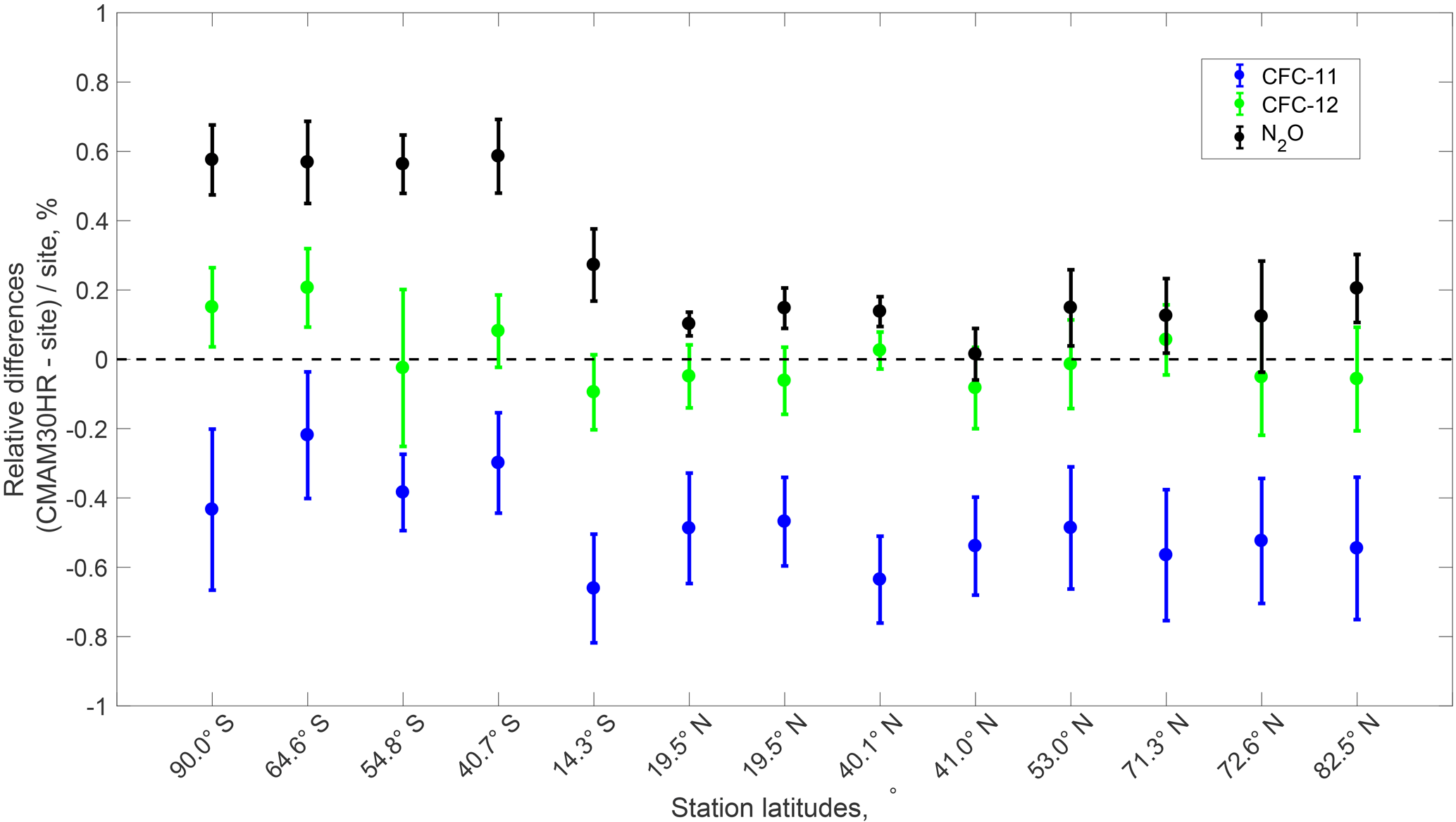
Figure 1Comparison of CMAM30HR simulations of CFC-11 (blue), CFC-12 (green), and N2O (black) to the HATS surface flask network of measurements at various locations around the world. Locations of measurement sites are indicated by latitude. Relative differences are calculated as the difference between the concentration at the surface site and the lowest model layer of the nearest neighbour grid box to the site in the CMAM30HR output, divided by the measured concentrations. The relative differences were calculated based on the monthly averaged observations and simulations. Shown here are the mean of the relative differences between May 2004 and June 2010 and the error bars indicate 1 standard deviation of the mean of the relative differences over the time period.
To ensure the consistency of the boundary conditions applied to the CMAM30HR simulation, the model output was compared to measurements at surface monitoring sites using data from the NOAA HATS program. The monthly mean measurements of N2O, CFC-11, and CFC-12 have been compared to the monthly mean in the CMAM30HR output between 2004 and 2010. Because of the way the surface boundary condition was imposed, each site was compared to the lowest model level of the closest grid point in the CMAM30HR output. The relative differences have been calculated by subtracting the measurement from the simulation and dividing by the measurement for each month in the time series. The differences over time were compared and no trend in the differences was observed. The comparisons of each trace gas at each site are summarized in Fig. 1, ordered by latitudinal location. Data included here are averaged over the 2004 to 2010 period and error bars (±) indicate 1 standard deviation.
Both CFC-11 and CFC-12 simulations have reasonably small differences, generally less than 1 %, from the surface measurements. Over the time period compared, CMAM30HR appears to underpredict CFC-11 at all HATS sites while the CFC-12 comparisons are not significantly different from zero within 1 standard deviation for all but two sites in the Southern Hemisphere. The N2O comparisons show that the model consistently overpredicts the concentrations at 11 of the 13 sites. There appears to be some latitudinal dependence in the comparisons of N2O which may be caused by the application of a globally averaged boundary condition in the run. Generally the differences for all the species shown are within ±1 %, which is to be expected since the model boundary conditions were derived from these measurements.
2.2.4 Influence of nudging on the age of stratospheric air
The mean age of stratospheric air, i.e. the average time elapsed since the last time an air parcel was in the troposphere, can provide a diagnostic for determining differences in isentropic transport and mixing between different model runs (Hall and Plumb, 1994; Waugh and Hall, 2002). The stratospheric age of air in the model is derived from an idealized SF6 tracer whose lower boundary condition linearly increases over time. In this section, the CMAM30, rather than CMAM30HR, mean age of air is used since no transport changes were made between the two runs of the model. Averaged between 2004 and 2010, Fig. 2a shows the zonal distribution of the CMAM30 mean age subtracted from the mean age from an identical, but freely running, version of the CMAM using the same specified sea surface temperatures and sea-ice data. The differences in age range from approximately −1.25 to +1 years, where the positive differences indicate areas where the air in CMAM is older than that in CMAM30, and the negative differences indicate areas in which the CMAM30 age is older than in the CMAM age. In general, the nudging of CMAM appears to affect the Southern Hemisphere more than the Northern Hemisphere. Below 50 hPa in the tropics and midlatitude regions, the difference between the age in the two versions of the model is close to zero. Above 50 hPa in the tropics and midlatitudes and above 150 hPa in the polar regions, air in CMAM is older than that in CMAM30, with peaks occurring around the surf zones in the stratosphere. This implies that for the majority of the lower stratosphere the process of nudging leads to an apparent decrease in the CMAM age of air. The cause of this has not been fully explained in the literature at this time; however, it can be speculated that nudging the model to the reanalysis could be a source of artificial drag that drives the BDC to be more rapid than in the free-running version of the model.
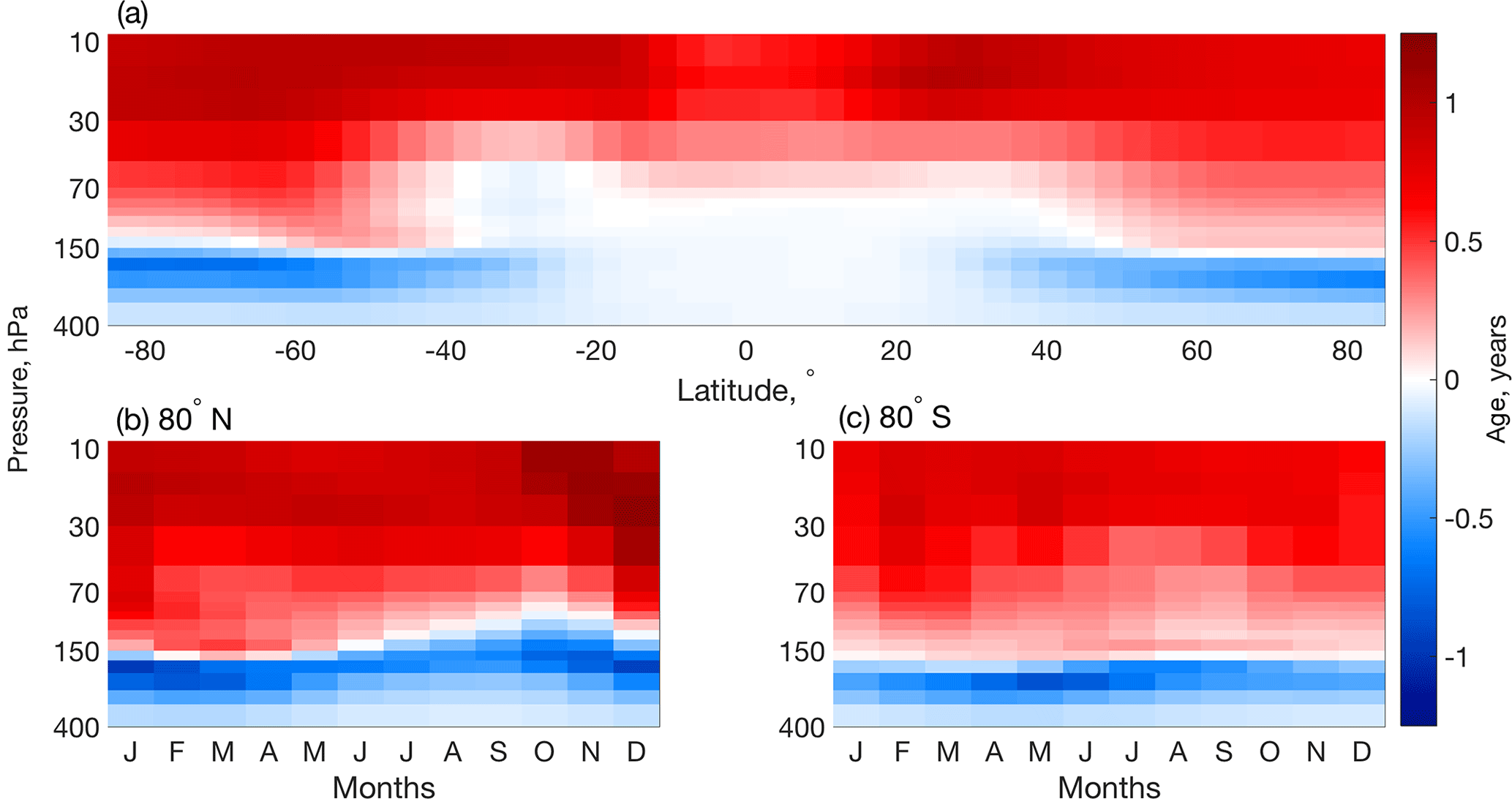
Figure 2A comparison of the age of stratospheric air in the free-running CMAM and CMAM30 averaged between 2004 and 2010. (a) The zonal mean difference of the CMAM30 mean age subtracted from the free-running mean age (years) and the monthly time series difference (b) at 80∘ S and (c) at 80∘ N.
In the polar regions of Fig. 2a, the comparisons exhibit a different behaviour in the lowermost stratosphere relative to the rest of the stratosphere. The differences are close to zero at the lowest pressure level shown (400 hPa). Above approximately 300 hPa, the CMAM30 air is older than the CMAM air and younger above approximately 150 hPa. These differences, while strongest at the latitudes poleward of 60∘, can extend to approximately 40∘ latitude in both hemispheres. Figure 2b and 2c show the monthly evolution at 80∘ S and 80∘ N, respectively. Below 150 hPa, the CMAM30 air appears to be older than the air in the free run and this tends to be pronounced during the respective summer months in each hemisphere. At 80∘ S, the pattern of differences in the age of air change in altitude over time. At approximately 150 hPa in May, the air in CMAM30 is older than the air in CMAM. This difference appears at approximately 100 hPa by October, with a larger magnitude. In November and December, during austral spring, the age difference remains such that the CMAM30 air is older than the air in CMAM. In Fig. 2c, the evolution of the differences in age of air at 80∘ N appears restricted to the same altitudes but the seasonal timing of the pattern is similar. The difference peaks in spring–summer and dissipates through the fall and winter. The prevalence of the older air in the polar lowermost stratosphere in the nudged run is significant because, throughout the stratosphere, air in CMAM30 is younger than that in CMAM. It is known that the freely running CMAM has a cold bias inside the Antarctic vortex. McLandress et al. (2012) suggest that there may be missing gravity wave drag (GWD) in the Southern Hemisphere based on comparisons of the free-running model simulations and reanalysis data. By effectively adding this missing GWD through the nudging to reanalysis data, downwelling between 70 and 90∘ S is increased, leading to higher temperatures – a reduction in the cold bias – during September and October. The increased downwelling pushes the older air deeper into the lowermost stratosphere, causing the observed differences in age between the two versions of CMAM.
In general, synoptic-scale waves are filtered out close to the tropopause and only planetary-scale waves can propagate further up into the stratosphere (Dickinson, 1969). Plumb (2002) showed that synoptic-scale wave drag drives the lower branch of the BDC, while the drag that drives the deeper parts of the BDC are associated with planetary wave drag. CMAM30 appears to reproduce the upper troposphere simulated in CMAM and, to some degree, the lower branch of the BDC as well. This is evidenced by the near-zero differences in Fig. 2a between 50∘ S and 50∘ N and between 100 and 50 hPa; however, the absolute ages in this region tend to be quite small. Understanding the impact of the nudging on the age of air provides the basis for an interpretation of the isentropic transport and mixing differences between the two model runs. While it is difficult to quantify the extent to which the differences in age of air would change tracer concentrations at a given location, it is necessary to consider these results when considering implications for the free-running model, particularly for the deep branch of the BDC. Based on Fig. 2, CMAM30 clearly has older air in the extratropical lowermost stratosphere. It is potentially caused by either stronger downwelling of the older air from above, consistent with a stronger BDC, or reduced isentropic mixing of tropospheric air from lower latitudes (e.g. Hegglin and Shepherd, 2007). Therefore, the differences in age appear to suggest a slower shallow branch or a faster deep branch of the BDC.
2.3 TLP model
A modified TLP model (Ray et al., 2016) is used to interpret the differences between the CMAM30HR simulations and the ACE-FTS measurements. The modified TLP is based on a set of three coupled one-dimensional equations relating transport between the tropics and each hemispheric extratropical region (Plumb, 1996; Neu and Plumb, 1999; Hall and Waugh, 2000). The model includes advection, vertical diffusion, and horizontal mixing between the extratropics and the tropics. Significant changes to the modified version of the TLP model include common pressure coordinates in all regions and the addition of particle trajectories with photochemistry. The modification was done to allow for direct comparisons between TLP output and other models and/or measurements. The Lagrangian approach is described by Ray et al. (2016). The tropical boundaries in the TLP model averages were chosen based on observational estimates of the upwelling region (Ray et al., 2016). The model was run with a vertical resolution of 200 m and a maximum altitude of 40 km above tropopause; however, the results included here are limited to 30 km in altitude above the tropopause. To ensure the effectiveness of the TLP as an interpretation tool, Ray et al. (2016) established that the TLP could accurately simulate the CMAM30HR output with its mean circulation and a TLP-derived mixing parameter as an input. The mixing parameter was derived from a suite of simulations conducted with the TLP at varying amounts of mixing. The resultant best match to the averaged 2004–2010 CMAM30HR CFC-11, CFC-12, and age of air profiles was the mixing efficiency selected to initiate the simulations. The TLP model is used here to identify the changes to the CMAM30HR tropical upwelling and effective mixing that may improve the comparisons between ACE-FTS and CMAM30HR by testing a range of tropical upwelling and mixing efficiency settings.
Diagnosing the biases in the model stratospheric circulation requires a complete separation of the effects of the strength of the BDC and mixing. A simplified model, such as the TLP, is useful to interpret differences between measurements and CCMs because of the complexity of wave activity contributing to stratospheric mean circulation and mixing. It would not be prudent to adjust model parameterizations in CMAM to modify wave breaking because many aspects of the model climatology would be impacted with no way of separating the effects (Ray et al., 2016). While the TLP-based analysis does not identify a specific mechanism, it can separate the contributions of model biases in the BDC and in mixing to biases in the resulting distribution of species.
3.1 Measurement–model comparison techniques
Two of the comparison techniques used in this study are described here: the first is the comparison of zonal means and the second is the computation of joint probability density functions.
3.1.1 Zonal mean comparison technique
To assess the transport and chemistry in CMAM30HR, measurements of N2O, CFC-12, and CFC-11 are compared with simulated concentrations in latitude-pressure coordinates. A common method of visualizing the distribution of long-lived trace gases is the zonal mean cross section. In this work, data from the ACE-FTS profiles, sampled CMAM30HR profiles, and the relative difference profiles were averaged in 5∘ latitude bins and over 18 pressure levels (equally distributed in the log of pressure from 450 to 10 hPa), corresponding to altitude ranges from approximately 5 to 30 km. In these plots, colour contours indicate the VMR of the species. The comparison of the ACE-FTS measurements and the subsampled CMAM30HR output is shown as the average of the differences, defined as CMAM30HR minus ACE-FTS divided by the ACE-FTS measurement. The altitude of the average thermal tropopauses is typically indicated by a black line. All measurements and subsampled model output between June 2004 and May 2010 have been included, representing an average of 6 years of observations and simulations.
3.1.2 Joint probability density functions
Tracer–tracer correlations have been used in a number of studies to identify transport and mixing characteristics in the stratosphere and to derive climatologies from sparse data (e.g. Plumb and Ko, 1992; Plumb, 1996; Toon et al., 1999; Sankey and Shepherd, 2003; Hegglin and Shepherd, 2007). Plumb and Ko (1992) showed that long-lived species exhibit compact correlations even with varying meteorological conditions, minimizing discrepancies resulting from sampling and daily variations; thus, sparse measurements, such as those from aircraft, can be useful in model assessment studies (e.g. Sankey and Shepherd, 2003). The correlations used here are N2O–CFC-11 and include only the stratospheric data available (data located at altitudes above 2 km above the thermal tropopause). The correlations produced from both the ACE-FTS measurements and CMAM30HR simulations exhibit compact relationships that tend to be densely populated. Determining whether the model can capture the clustering in addition to the overall shape is important to understanding whether the stratosphere is well-reproduced by the model. Understanding the density distribution of a dataset is particularly useful for tracer–tracer relationships with compact correlations. Following the methods of Sparling (2000) and Hegglin and Shepherd (2007), normalized joint probability density functions (JPDFs) have been calculated for the ACE-FTS and CMAM30HR correlations described above. JPDFs are two-dimensional histograms that reveal the clustering of data (Hegglin and Shepherd, 2007) and can be used to test how well a model captures the behaviour of trace gases in the stratosphere. Hegglin and Shepherd (2007) have shown the impact of ACE-FTS measurement uncertainties in JPDFs by comparing the full model output, subsampled model output, and ACE-FTS measurements. They found that there was larger variability in the ACE-FTS JPDFs compared to those of the subsampled CMAM output.
3.2 The influence of beta angle
ACE-FTS records a series of spectra along a slanted path line of sight during each occultation. The length of this slanted path is different for each occultation. Each ACE-FTS occultation is assigned a latitude and longitude at the 30 km tangent point, geometrically calculated (Boone et al., 2005, 2013). A sample year of the geometric 30 km tangent point latitudes is provided in Fig. 3 (black circles), showing the annual repeating latitudinal coverage. The beta angle parameter, a measure of the angle between the solar vector and the satellite orbit plane, has also been included in Fig. 3 (red circles). The beta angle is an important parameter to consider because as it changes, so does the geographic distance between each spectrum acquired through the profile of any given occultation. The distance is greatest at high beta angles (both positive and negative), which occur when ACE is in view of the sun for longer periods. Since the FTS instrument measurement frequency is held at a constant 2 s interval, more measurements per profile and longer ground-paths of the retrieved profile occur at high beta angles.
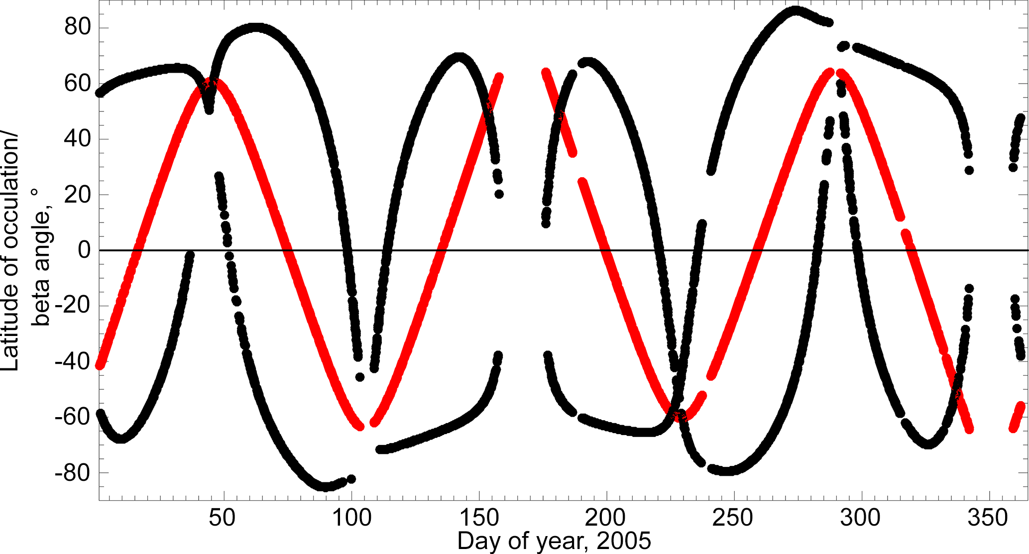
Figure 3The ACE-FTS sampling pattern for the year 2005. Each black circle is the latitude of the 30 km tangent height of an occultation and each red circle is the corresponding beta angle of the occultation.
Considering the impact of observation sampling is a critical step when comparing measurements with model output. The work of Toohey and von Clarmann (2013), Toohey et al. (2013), and Millán et al. (2016) illustrate the necessity for considering the sampling patterns resulting from different measurement techniques and satellite orbits. The ground path length of a profile is considered because a single profile can be representative of more than one geographic region, typically varying more over latitude than longitude. A refraction model is used to determine the geographic locations along the slant path of the ACE-FTS profiles (Boone et al., 2005, 2013). At the 30 km tangent altitude, it has been found that for 98 % of the ACE-FTS occultations, the difference between the geometric latitude and the refraction calculation is less than 0.2∘. A useful marker of a nominal occultation length is at a beta angle of 53∘, corresponding to an occultation duration of 3 min. Occultations longer than 3 min, at beta angles larger than 53∘, measure across large spatial distances and represent approximately 12 % of the ACE-FTS data used in this work. Both horizontal and vertical variations within the CMAM30HR output will impact the comparison to ACE-FTS measurements. The CMAM30HR fields are output on a grid with a spatial resolution of approximately 400 km. While most ACE-FTS occultations have a shorter horizontal extent than the CMAM30HR grid point footprints, there are some occultations that fall outside of a single grid point range in the upper troposphere and lower stratosphere. For example, between 5 and 30 km, 15 % of occultations extend across more than one CMAM30HR grid point footprint, of which 82 % are at beta angles greater than 53∘ and 80 % are at latitudes poleward of 30∘. Various model sampling techniques have been investigated since occultations span multiple grid point footprints in both latitude and longitude, as well as vertically.
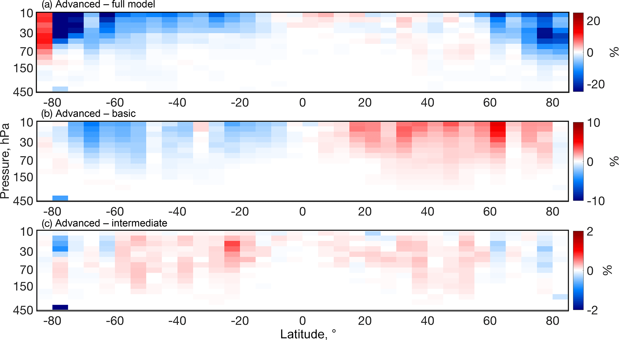
Figure 4The comparisons of the three sampling methods described in the text using N2O simulations in CMAM30HR. The relative differences (%) defined as the difference between the advanced sampling and (a) the full model output, (b) basic sampling, and (c) intermediate sampling, relative to the advanced sampling. Note the different colour scales in each panel.
3.3 Comparison of sampling techniques
To determine the impact of sampling the model output at varying levels of detail, three methods were tested by sampling the full model output (the CMAM30HR output at all latitudes and longitudes for each 5∘ latitude bin) between June 2004 and May 2010. All three methods began with identifying the temporally coincident three-dimensional CMAM30HR output (latitude, longitude, pressure) for each ACE-FTS profile; the output within 3 h of the occultation was selected with no temporal interpolation. The three-dimensional output was interpolated in the vertical dimension to the ACE-FTS profile pressure grid, which is different for each occultation since the retrievals are provided on an altitude scale. The “basic” sampling method involved selecting a vertical column based on the nearest neighbour grid point to the 30 km tangent point location with no interpolation and no consideration of the vertical extent of the profile. The “intermediate” level of sampling extracted the vertical column based on a bilinear interpolation of the four closest grid points to the 30 km geometric tangent point but with no consideration of the variation in geographical location of the tangent points above or below 30 km. The “advanced” sampling method improves on the intermediate level of sampling by performing the bilinear interpolation at each level of the ACE-FTS profile using the distinct geographic locations, derived from the refraction model (Boone et al., 2005, 2013), for the respective level. Therefore, at each vertical level in the ACE-FTS profile, a spatial bilinear interpolation including the four geographically closest grid points was computed to determine the comparable CMAM30HR VMR. To illustrate the sampling effect between 450 and 10 hPa (5–30 km), the differences, relative to the advanced technique, in the zonal mean of N2O over the observation period (June 2004–May 2010) are compared in Fig. 4. The advanced method is compared to the full output of the model (Fig. 4a), the basic model sampling (Fig. 4b), and the intermediate sampling (Fig. 4c).
The comparison of the advanced sampling and full model output in the stratosphere is dominated by the influence of the polar vortex in both hemispheres. Generally, there is good agreement throughout the troposphere, with less than 5 % differences. For the long-lived tracers investigated in this work, the free troposphere is well mixed such that there is minimal influence of the ACE sampling pattern. In the stratosphere, however, there are pronounced differences on the order of 20 %. Air in the polar vortex is typically composed of older air brought down from higher altitudes. Therefore, tracer concentrations within the vortex and vortex edge tend to be significantly different from those in the midlatitude surf zone during the winter in each hemisphere. The differences seen in Fig. 4a occur because comparing the full output to measurement-like samples of the output accounts for neither the variability of the vortex edge in both longitude and latitude nor the differences in spatially and temporally sampled large-scale downwelling of air within the vortex compared to a zonal mean average that includes the model simulation at all longitudes and time periods. At the edge of the vortex, tracer concentration gradients are strong, so comparing measurements to the full output of the model will tend to smear the influence of the vortex on tracer concentrations. The differences are not symmetric latitudinally due to different dynamical conditions in each hemisphere. For example, in the Antarctic stratosphere in September there is a strong decrease in the geographic extent of the polar vortex with height such that the vortex is much wider geographically at 100 hPa than at 10 hPa. A similar phenomenon occurs in the Arctic but it is much more variable both spatially and vertically.
The advanced sampling technique is compared to the basic sampling in Fig. 4b. The distinction between Fig. 4a and b is that rather than using the full model output, the nearest grid point is selected based on the geographic location of the 30 km tangent point of the ACE-FTS measurements. Even this basic level of sampling improves the comparison in the stratosphere substantially, bringing the range of differences down to ±10 %. It is worth noting that the stratospheric differences in the midlatitudes are on the same order of magnitude with a similar latitudinal pattern but of opposite sign. The differences of 5–10 % are primarily negative in the stratosphere in the Southern Hemisphere and positive in the Northern Hemisphere. This pattern occurs because each ACE-FTS profile is tilted such that the top of the profile is always further north than the bottom of the profile, leading to a directional bias. In the Northern Hemisphere, profiles tend to “point” toward the North Pole, and therefore measurements in this hemisphere are subject to a poleward bias. In the Southern Hemisphere, profiles point toward the Equator, leading to an equatorward bias in sampling. Therefore, the choice of “closest” grid point likely biases the comparisons, leading to the differences in Fig. 4b.
Figure 5 illustrates the average latitudinal extent of occultations between the 5 and 30 km tangent altitudes (where, for an individual occultation, the latitude at 5 km is subtracted from the latitude at 30 km), showing the two directionalities for each 5∘ latitude bin included in Fig. 4b, with error bars indicating 1 standard deviation from the mean latitudinal extent. A poleward bias implies that the 30 km tangent point is located poleward of the 5 km tangent point and an equatorward bias reflects when the 30 km tangent point is located equatorward of the 5 km tangent point.
In the midlatitude region of the Northern Hemisphere, the average latitudinal extent of occultations exhibits a primarily poleward bias while the occultations in the southern hemispheric midlatitudes exhibit a primarily equatorward bias. The northern hemispheric poleward bias in Fig. 5 corresponds to the positive differences in the northern hemispheric midlatitude stratosphere in Fig. 4b and the southern hemispheric equatorward bias corresponds to the negative differences in the southern hemispheric midlatitude stratosphere. The comparison to the advanced technique in Fig. 4b reflects the combined influence of the horizontal interpolation and, to a lesser degree, the geographical extent of the ACE-FTS profiles. In the Northern Hemisphere, contributions from sampling the model at lower latitudes (which tend to have a higher concentration) lead to positive differences between the two sampling techniques; in contrast, in the Southern Hemisphere, contributions from sampling the model at higher latitudes (lower concentrations) lead to negative differences between the advanced and basic sampling techniques. This nuance in the sampling pattern highlights the importance of considering the sampling pattern of the ACE-FTS occultations when comparing measurements to model output.
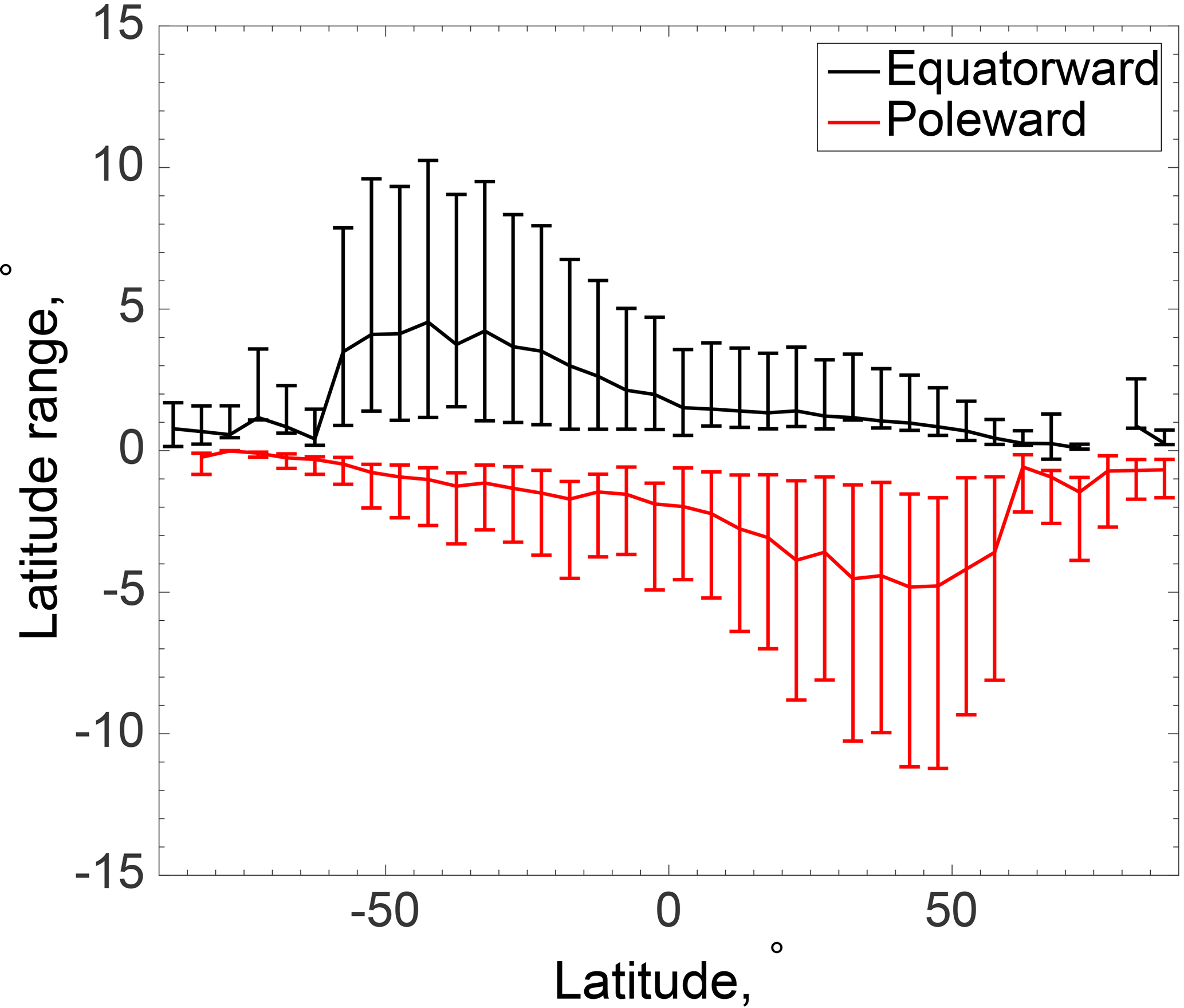
Figure 5Average latitude ranges covered by ACE-FTS occultations in a given 5∘ latitude bin, separated by an equatorward bias (black) and a poleward bias (red) as defined in the text. The error bars indicate 1 standard deviation from the mean latitudinal extent for the given 5∘ latitude bin.
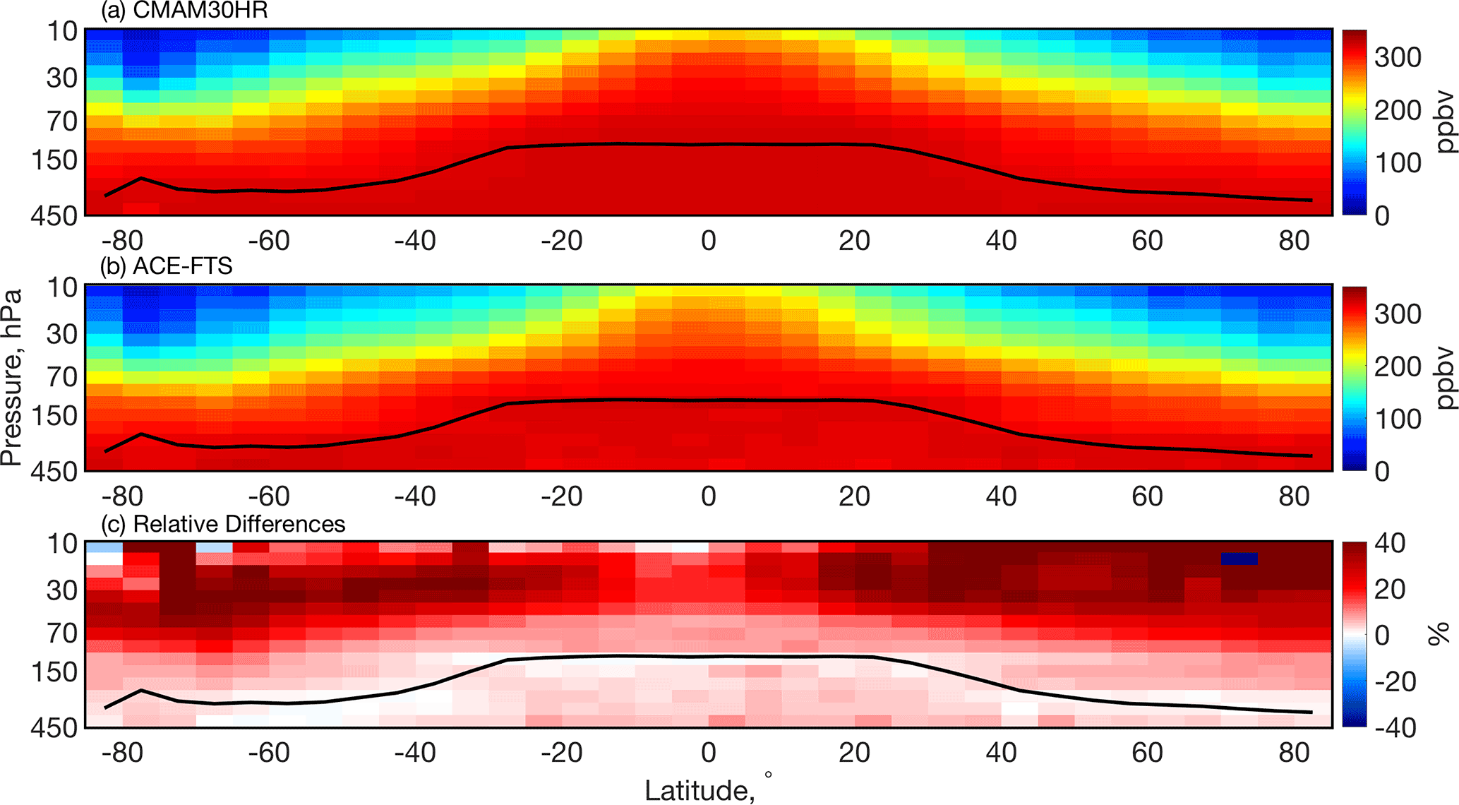
Figure 6Zonally averaged annual-mean latitude-altitude distributions of N2O: (a) CMAM30HR (ppbv), (b) ACE-FTS (ppbv), and (c) the mean relative difference (in %) between sampled model and ACE-FTS profiles, divided by the ACE-FTS profiles (100 × (CMAM30HR − ACE-FTS) ∕ ACE-FTS). The black line indicates the location of the thermally defined tropopause.
Figure 4c compares the advanced and the intermediate sampling. With approximately ±2 % differences between the two techniques, it is clear that the intermediate sampling technique can account for much of the geographic extent of the ACE-FTS profiles at this model resolution. However, if comparing to a model with a finer resolution or if a larger vertical extent is considered, accounting for the full geographic extent of the profile will become more important. The more detail that is included in the sampling of the model, the more comparable the output is to the observations. The advanced method of sampling provides the most appropriate model profiles for direct comparison between ACE-FTS and CMAM30HR. Therefore, all comparison results shown in this study utilize CMAM30HR output that has been sampled using the advanced technique.
4.1 General features of tracer morphology comparisons
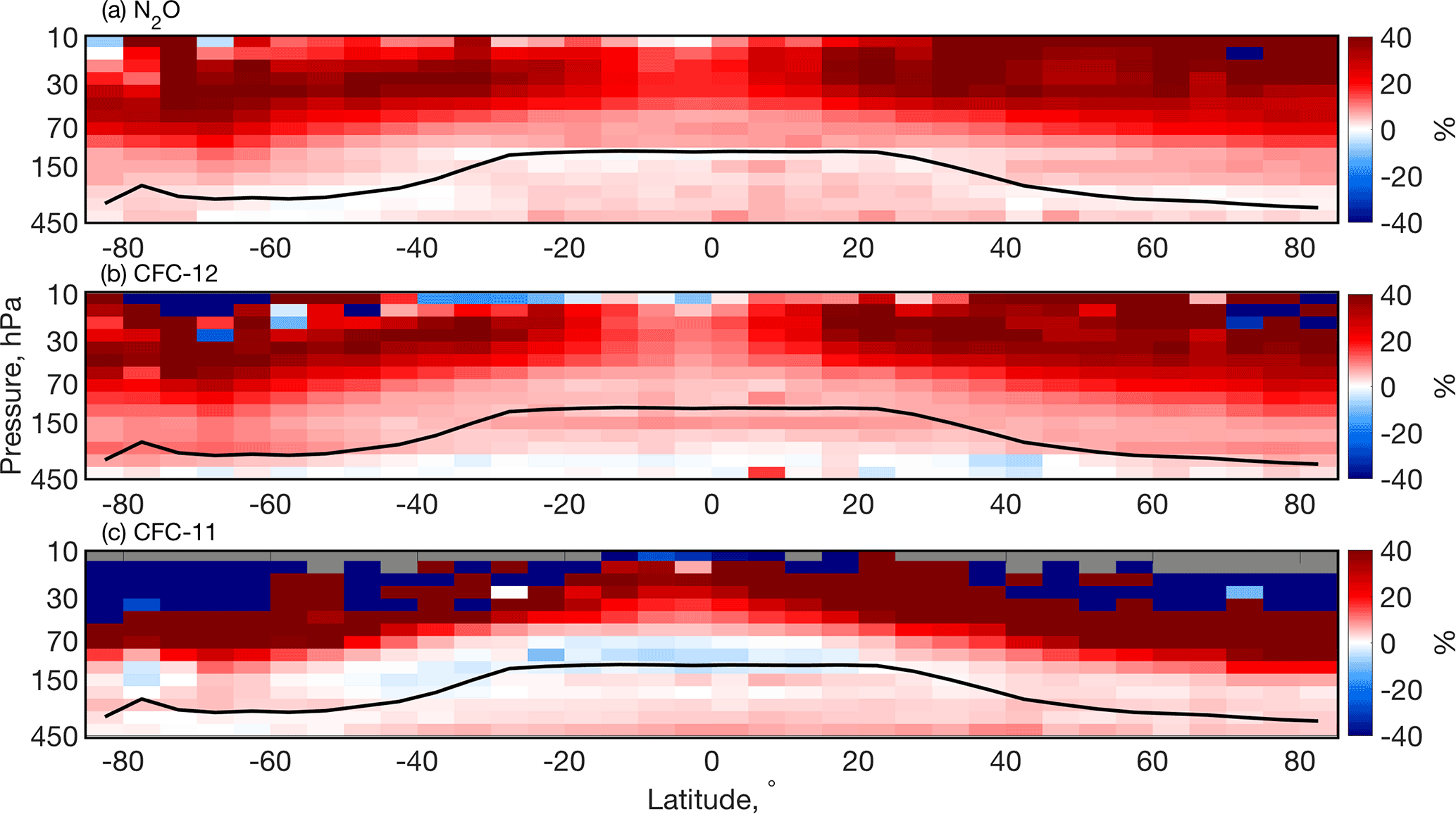
Figure 7Same as Fig. 6c for (a) N2O, (b) CFC-12, and (c) CFC-11. The grey regions indicate where no data are available.
The zonally averaged annual-mean distribution of N2O is presented in Fig. 6. The N2O simulated by CMAM30HR is shown in Fig. 6a, the ACE-FTS measurements are shown in Fig. 6b, and the average of the profile differences within each 5∘ latitude bin is shown in Fig. 6c. Both the ACE-FTS measurements and the CMAM30HR distribution of N2O in Fig. 6 show many of the features that are expected of a long-lived tracer with a tropospheric source and chemical losses that occur primarily in the stratosphere. The distributions show a decrease in concentration of N2O with altitude at all latitudes and also moving from the Equator poleward at each pressure level and in each hemisphere. There is a hemispheric asymmetry in the decrease with altitude beyond the tropical region. The southern extratropical and Antarctic concentrations of N2O tend to decrease with altitude more rapidly than those in the Northern Hemisphere. This asymmetry is likely driven by differences in the isolation of the polar vortex in each hemisphere and the large-scale downwelling that is largely dependent on this isolation. By visual comparison, the lowest concentrations observed and simulated appear to be in the Antarctic region between 30 hPa and 10 hPa and the Arctic stratosphere above 20 hPa. The quantitative comparison between the ACE-FTS and CMAM30HR zonal mean N2O distributions in the bottom panel of Fig. 6 reveals significant differences throughout the lower stratosphere, with the largest differences in the northern polar region. CMAM30HR simulates larger concentrations of N2O in the lower stratosphere. Upwelling in the tropics, descent in the extratropics, and mixing in the surf zone define the transport controls on the distributions in the stratosphere. The differences observed in Fig. 6c are influenced by the combined effects of these features on the measured and the simulated concentrations of N2O. Therefore, if there were no issues in the simulated stratospheric transport, the differences would be of similar magnitude to the upper troposphere comparisons (less than ±5 %), unless there was a significant flaw in the chemical losses in the model.
Investigating measurement–model comparisons using more than one trace gas leverages the varying lifetimes of and chemical processes of each gas. The comparisons of CMAM30HR and ACE-FTS, equivalent to the bottom panel of Fig. 6, are shown in Fig. 7a–c for N2O, CFC-12, and CFC-11, respectively. Each of the panels shows the differences as a percentage. All three species show good measurement–model agreement (within approximately 5 %) in the well-mixed troposphere. In the tropics, the VMRs of these three species remain relatively constant up into the lower stratosphere where chemical loss processes begin to break down the compounds. Above 70 hPa in the tropics, the CFC-12 and N2O comparisons show similar agreement (on the order of 5 %). However, above 50 hPa in the tropics, CFC-11 exhibits both positive and negative differences between the measurements and model simulations. These differences in CFC-11 are also observed outside the tropics above 70 hPa and are much higher (on the order of 50 %). In the northern hemispheric extratropics, the differences are primarily positive but become more variable closer to the northern polar region. Very small concentrations above 70 hPa, which occur because of the significant photolytic losses in the tropical lower stratosphere, lead to the large magnitude of the differences in CFC-11. The irregular pattern in the CFC-11 differences is driven by the variability in the measurements as ACE-FTS reaches its detection limit.
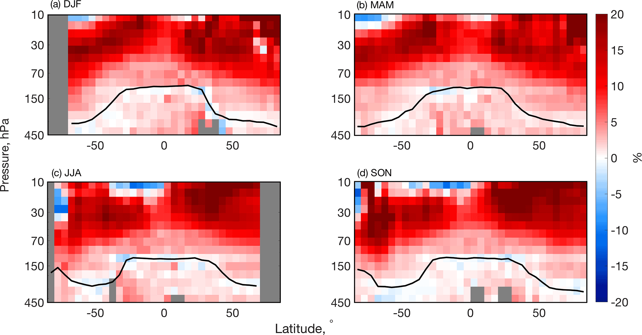
Figure 8The relative mean of individual ACE-FTS profiles subtracted from CMAM30HR profiles of N2O, divided by the ACE-FTS measurements for each season: (a) December–January–February (DJF), (b) March–April–May (MAM), (c) June–July–August (JJA), and (d) September–October–November (SON). The grey regions indicate where no data are available.
4.2 Seasonality of the tracer morphology comparisons
The structure and intensity of the BDC varies seasonally. In general, the BDC is strongest in the northern hemispheric winter because of wave-driven enhancements initiated by topography and because, during this time of year, climatological westerlies facilitate wave propagation into the stratosphere (e.g. Rosenlof, 1995; Plumb and Eluszkiewicz, 1999). It is well known that tropical upwelling is stronger in the summer hemisphere; therefore, during the December–January–February (DJF) season the upwelling is strongest in the Southern Hemisphere (e.g. Yulaeva et al., 1994). Investigating the comparisons between the CMAM30HR simulations and the ACE-FTS observations in a seasonal context helps to determine whether the differences observed earlier are related to the behaviour of the BDC. If the differences observed in Fig. 7 are driven by the simulation of the BDC in the model, it would be expected that the morphology of the seasonal differences would appear to follow the behaviour of the BDC.
For each season, Fig. 8 identifies the differences between the simulation and the measurements. The seasonal composites shown here do not fully represent the seasons because of the sampling pattern of the ACE-FTS (recall Fig. 3). However, the comparisons are relevant since the CMAM30HR output has been subsampled, as previously described. The most obvious features across all seasons in Fig. 8 are the same as those of the differences shown in Fig. 7a. There is good agreement in the lower stratosphere at all latitudes and in the tropics up to about 50 hPa. In the mid-stratosphere, CMAM30HR simulates higher concentrations of N2O than those measured by ACE-FTS. Some of the largest differences occur at the high northern latitudes during boreal winter and spring, presumably in the region of downwelling within the polar vortex.
The large disagreements in the north polar region during winter and spring indicate that the downwelling portion of the BDC across the different seasons is not well characterized by CMAM30HR. Meanwhile, the shifting of the agreement in the tropical region through the seasons indicates that the simulation is consistent with the spatial distribution of the observations in this region. For example, the difference in the southern tropical latitudes appears small (close to 0 %) up to 50 hPa and to approximately 40∘ S in DJF, but the agreement diminishes in this region in the March–April–May (MAM) season, presumably when the tropical upwelling begins to decline in strength and shift toward the Equator. A similar pattern is observed in the Northern Hemisphere during austral winter where the differences in the northern tropical latitudes appear to be small up to 50 hPa and to approximately 40∘ N in the June–July–August (JJA) and September–October–November (SON) seasons. These results support the understanding that the most rapid tropical upwelling occurs in the summer hemisphere as first reported by Yulaeva et al. (1994).
In the comparisons shown in Fig. 8, the northern high latitudes measurement–model differences are significantly different compared to those in the southern high latitudes. There are negative differences at high southern latitudes in MAM, JJA, and part of SON. The differences seem quite asymmetric when compared with the results for the Northern Hemisphere. The negative differences at high southern latitudes appear to descend between MAM and JJA and begin to weaken in SON with the vortex breakdown. There is also some asymmetry in the differences between 30 and 10 hPa between the Northern and Southern hemispheres, particularly in winter for each hemisphere. These differences are likely due to the behaviour of the polar vortex in each hemisphere. In particular, the differences may be related to the model's (either CMAM30HR or the ERA-Interim reanalysis used for the nudging or both) ability to represent transport processes in the strong, cold, quiescent Antarctic vortex versus the warmer and more variable Arctic vortex.
Since the model run compared here has been nudged to the ERA-Interim meteorology, it cannot be simply concluded that the differences are due to the variable nature of the vortex. The vertical migration of the negative differences in the southern polar region across MAM, JJA, and SON suggests the vortex variability physical or chemical mechanism as the cause. The negative differences mean that there is an underprediction in the CMAM30HR simulation, which could happen if air that is too old is brought down into the vortex. As the vortex forms in fall, the negative differences appear and descend through the winter, reaching a maximum latitudinal extent. The appearance of the negative differences in the comparison of N2O between the observations and the model is conspicuous because elsewhere N2O is higher in CMAM30HR throughout the lower and middle stratosphere.
In Fig. 8b and d, the large positive differences in the northern hemispheric stratosphere may be caused by too much orographic wave driving in CMAM30HR (and CMAM30). This would lead to air moving from the tropical region into the extratropics and polar regions too quickly, thereby simulating higher than expected concentrations of N2O in the northern hemispheric stratosphere.
It is well understood that quasi-horizontal mixing flattens tracer isopleths in mixing regions and sharpens gradients at mixing barriers (e.g. Plumb, 2002). However, it can be very difficult to separate the effects of mixing barriers from the residual circulation when looking at zonal mean comparisons between measurements and models. Therefore, it is necessary to scrutinize mixing barriers individually.
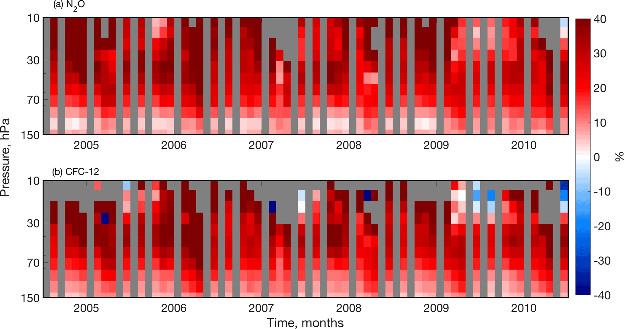
Figure 9A monthly time series of the average relative differences between the model and the measurements (CMAM30HR minus ACE-FTS, divided by ACE-FTS), as in Fig. 6c for (a) N2O and (b) CFC-12 in the Northern Hemisphere (60–90∘ N) between June 2004 and May 2010. The grey regions indicate where no data are available.
5.1 The polar vortex
Consideration of the behaviour of the polar vortex in both hemispheres is necessary as they have atmospheric processes that affect their behaviour differently over time. For this purpose, the monthly mean differences between ACE-FTS and CMAM30HR over the time period of the study have been determined for the stratospheric abundances of N2O and CFC-12. CFC-11 has been excluded from this comparison because the limited vertical extent of the sensitivity of the measurement results in too few data in the stratosphere. All comparisons shown here are profiles located poleward of 60∘ and show the mean of the difference between the ACE-FTS and CMAM30HR profiles, relative to the ACE-FTS profile. The comparisons here extend the work of Pendlebury et al. (2015), who discussed the polar region simulations in CMAM30 extensively by comparing temperature, ozone, methane, and water vapour up to 0.001 hPa with a variety of satellite instruments including ACE-FTS. All the species investigated in Pendlebury et al. (2015) have much shorter lifetimes than those of N2O and CFC-12. The advantage of using species with long lifetimes is that at least some of the parcels of air that are sampled have been through the deep branch of the BDC. By restricting comparisons to the polar stratosphere, it is primarily air from the deep branch of the BDC that is being investigated. Tracers with a stratospheric sink are mostly depleted from the deep branch because they have had the most time for chemical loss to occur since they entered the stratosphere.
The comparison of the N2O and CFC-12 difference time series (Fig. 9) demonstrates that there is interannual variability that is consistent between the two gases in the Arctic. While the two species shown follow similar patterns over time, there appear to be larger differences in the CFC-12 comparison than in the N2O comparison. There are two possible (and related) reasons for this difference: the range in the concentrations of CFC-12 is much larger than that of N2O, and there are differences in their respective chemical losses. For example, the photolysis loss of CFC-12 is faster than that of N2O throughout much of the stratosphere, as evidenced by the differences in their lifetimes (102 years for CFC-12 and 123 years for N2O). Generally, it appears that the model simulates higher concentrations of both species compared to ACE-FTS measurements through much of the stratosphere, with the largest differences occurring above 30 hPa. When the concentration of either tracer becomes very small (typically air that has descended from the upper stratosphere or mesosphere), the relative differences between ACE-FTS and CMAM30HR can be enhanced. These differences are most clear in the N2O comparisons during the autumns of 2004 and 2009 and the springs of 2007 and 2010; in contrast, in the CFC-12 comparisons, the springs of 2005, 2006, and 2008 exhibit additional occurrences of this feature.
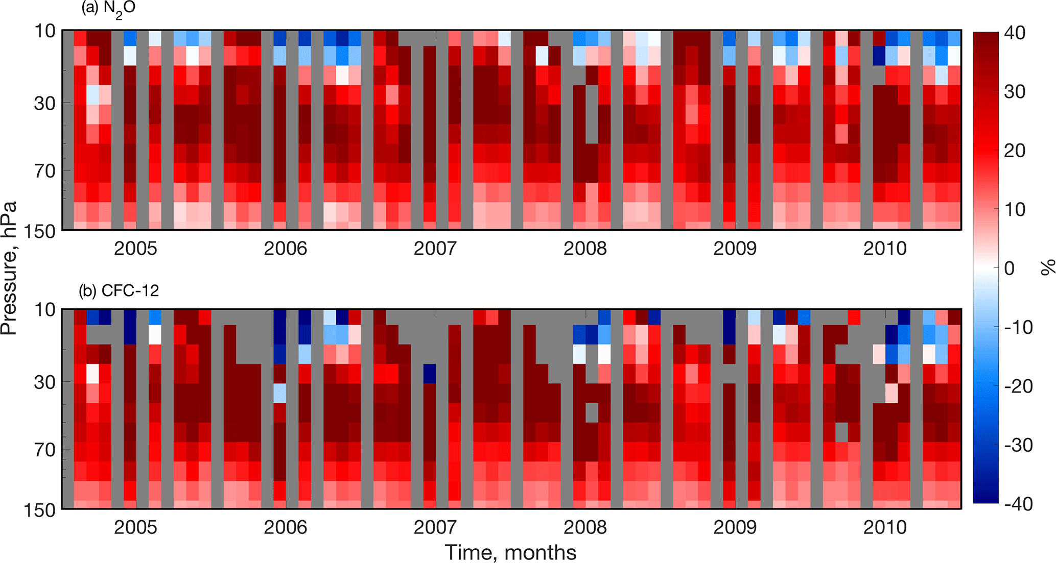
Figure 10A monthly time series of the average relative differences between measurements and the model (CMAM30HR minus ACE-FTS, divided by ACE-FTS), as in Fig. 6c for (a) N2O and (b) CFC-12 in the Southern Hemisphere (60–90∘ S) between June 2004 and May 2010. The grey regions indicate where no data are available.
During each of these periods, ACE-FTS observed much lower concentrations compared to CMAM30HR. Both the speed and structure of the residual circulation within the CMAM30HR run can contribute to the observed differences. It is possible that the BDC in the CMAM30HR simulation is drawing air through the deep branch of the BDC too rapidly. The vertical structure of the differences observed in Fig. 9, particularly between 70 and 30 hPa, may be caused by ACE-FTS measuring a descent in the air mass that CMAM30HR does not simulate. It is more likely that the model circulation is not moving enough air through the loss region of these tracers and through to the polar vortex. For photolytic tracers, the structure of the circulation is more important than the speed of the residual circulation because photolysis rates are so fast. Above a certain level in the stratosphere, the tracer is completely destroyed when air passes through the region. The distribution of photolytic species is a mixture of air that passed through the region of rapid loss and the air that by-passed the loss processes. This result is consistent with the work of Pendlebury et al. (2015), where they found large differences in temperature and ozone between satellite observations and CMAM30.
There is less interannual variability in the Southern Hemisphere comparisons (Fig. 10) than in the Northern Hemisphere (Fig. 9). This is expected since the variability of the southern polar stratospheric dynamics is much less than that in the northern polar stratosphere. However, the magnitude of the differences between the measurements and simulations is larger in the Antarctic stratosphere than in the Arctic stratosphere. Moreover, while the patterns of the differences in N2O and CFC-12 are quite similar in Fig. 10a and b, the magnitude is more pronounced in the CFC-12 comparisons. The largest differences occur above 30 hPa where the concentrations of CFC-12 are extremely low. The peak in the magnitude of the CFC-12 differences appears to increase in vertical extent through the austral springtime. The largest differences tend to occur during summer (December) at around 40 hPa for both tracers. The differences in CFC-12 are established at the top of the vortex in July and propagate down until vortex breakup in December. However, this propagation does not occur to the same extent in the N2O comparisons, which may be a reflection of the differences in the chemistry of the two tracers. For example, a source of N2O in the lower thermosphere has recently been identified in ACE-FTS measurements by Sheese et al. (2016). The N2O source descends into the mesosphere and stratosphere, thereby influencing air that is circulated in the BDC (Sheese et al., 2016). The transport of enhanced N2O downwards from the upper atmosphere has also been detected by Funke et al. (2008a, b). The CMAM30HR does not include this source of N2O. The results presented here are consistent with the methane comparisons discussed in Pendlebury et al. (2015). Generally, the descent of the model's high bias is observed in both hemispheres for all three trace gas species. The results of Pendlebury et al. (2015) indicate that the high bias is consistent with a fast BDC and that the downward propagation of the bias is a problem with the parameterizations in the model above 10 hPa.
5.2 The extratropical tropopause
The transport barrier at the extratropical tropopause can be permeable, allowing the exchange of air between the troposphere and the stratosphere. Understanding how CMAM30HR simulates this exchange assists in the interpretation of mixing effectiveness in the model and the impact of its finite resolution on the comparisons. Since ACE-FTS predominantly samples the polar regions and has fewer samples of extratropical latitudes, interpreting latitudinal or seasonal dependence of the exchange of air across the tropopause in the full atmosphere using these measurements must be considered from a tropopause coordinate perspective (Hegglin et al., 2009). In this study, a diagnostic of the tropopause barrier has been developed for comparison between the simulations and the measurements. The tropopause height, used in this analysis to define tropospheric air and stratospheric air, is the thermally defined tropopause based on the derived meteorological products for ACE-FTS (Manney et al., 2007) and based on sampled temperature profiles from CMAM30 output for the CMAM30HR simulations.
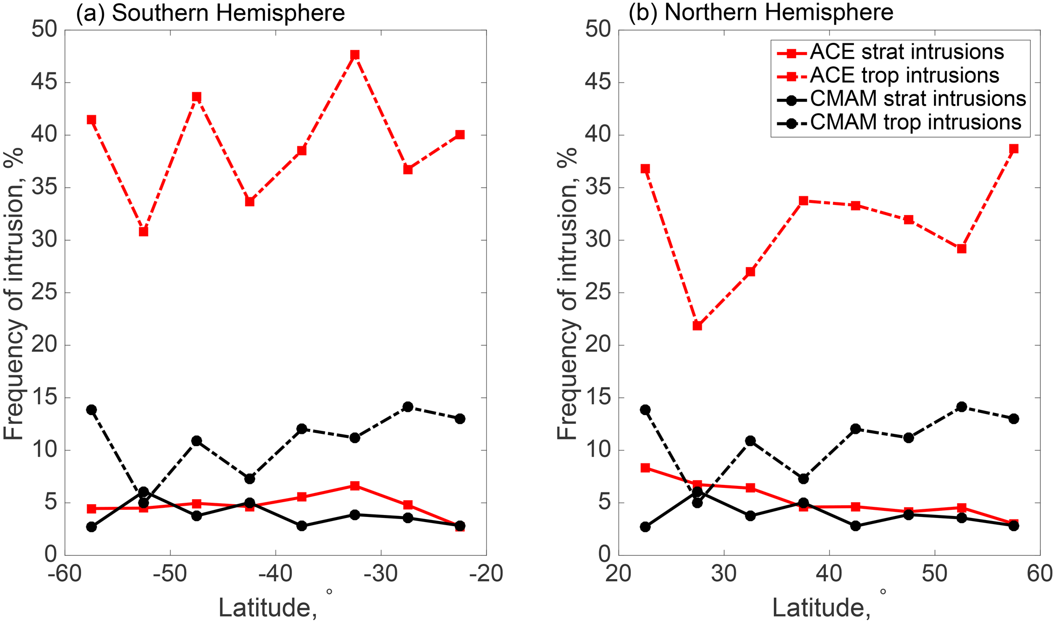
Figure 11The frequency of intrusion across the tropopause for both CMAM30HR (black circles) and ACE-FTS (red squares) below the 420 K potential temperature isotherm in (a) the southern hemispheric and (b) the northern hemispheric extratropical region between 20 and 60∘ N/S, respectively. For each 5∘ latitude bin, the frequency of intrusion events are separated by stratospheric intrusions (solid lines), where stratospheric-like air is found in the troposphere, and tropospheric intrusions (dashed lines), where tropospheric-like air is found in the stratosphere.
Since CFC-11 has a strong vertical gradient in concentration in the stratosphere, it can be used as a proxy for determining the exchange of air across the tropopause. The diagnostic developed for this analysis is the frequency of intrusions, which signifies the frequency of stratospheric (tropospheric) air penetrating into the troposphere (stratosphere). A data point is defined as an intrusion based on two criteria: the physical location of data point and the concentration relative to a tropospheric concentration threshold and only data below the 420 K potential temperature layer of the atmosphere have been considered. The tropospheric threshold was defined separately for each hemisphere as the tropospheric mean minus 1.5 times the tropospheric standard deviation. An intrusion frequency metric has been developed for comparison between the simulated and observed concentrations. A tropospheric intrusion is identified when a measurement is physically located in the stratosphere but its concentration is larger than the tropospheric threshold. A stratospheric intrusion is identified when a measurement is physically located in the troposphere but its concentration is smaller than the tropospheric threshold. For each 5∘ latitude bin between 20 and 60∘ latitude (N and S), the frequency of tropospheric and stratospheric intrusions have been determined. This technique was used to calculate frequencies for both the ACE-FTS measurements and CMAM30HR profiles.
The comparison of ACE-FTS and CMAM30HR tropospheric and stratospheric intrusions within the southern and northern extratropical latitudes is shown in Fig. 11a and b, respectively. There appears to be better agreement for the stratospheric intrusion comparisons and at some latitudes there is very good agreement between ACE-FTS (red) and CMAM30HR (black). However, there are some latitudes, such as 30–40∘ S and 20–25∘ N, where the stratospheric intrusions identified in the simulation are a factor of 2 fewer than those from the ACE-FTS measurements. In general, isentropes that are in the extratropical lowermost stratosphere are in the troposphere in the tropics (e.g. Holton et al., 1995). Fast isentropic transport occurs because wave motions cause air to rapidly change latitude, leading to the transport of stratospheric air into the troposphere. Since the disagreement in measured stratospheric exchanges is largest at latitudes where this isentropic transport tends to occur implies that CMAM30HR is not capturing this mechanism well or simply lacks the resolution to fully resolve the stratospheric intrusions features.
Based on Fig. 11, tropospheric intrusions occur more frequently in the ACE-FTS data than stratospheric intrusions and vary more significantly in number across the latitudes in both hemispheres. Additionally, the differences between the measurements and simulations are larger than for the stratospheric intrusions. It is possible that there is more tropospheric air found in the stratosphere with this method than stratospheric air found in the troposphere because tropospheric CFC-11 is more easily distinguishable. The manner in which the intrusions have been defined here does not rule out stratospheric air being identified as tropospheric if there is rapid, poleward transport out of the lower tropical stratosphere. Schwartz et al. (2015) suggest that it is easier to distinguish tropospheric intrusions into the stratosphere using tropospheric tracers and stratospheric intrusions into the troposphere using stratospheric tracers. Tropospheric CFC-11 concentrations found in the stratosphere at extratropical latitudes indicate air that likely has not cycled through the BDC because the air parcels have not experienced any loss processes that can only happen in the stratosphere, while stratospheric air in the troposphere could be representative of a range of aged air. For example, this air could have cycled through the BDC very quickly by re-entering the troposphere in the subtropics or it could have gone through the deep branch, allowing it to be more depleted and therefore more identifiable as stratospheric-like air.
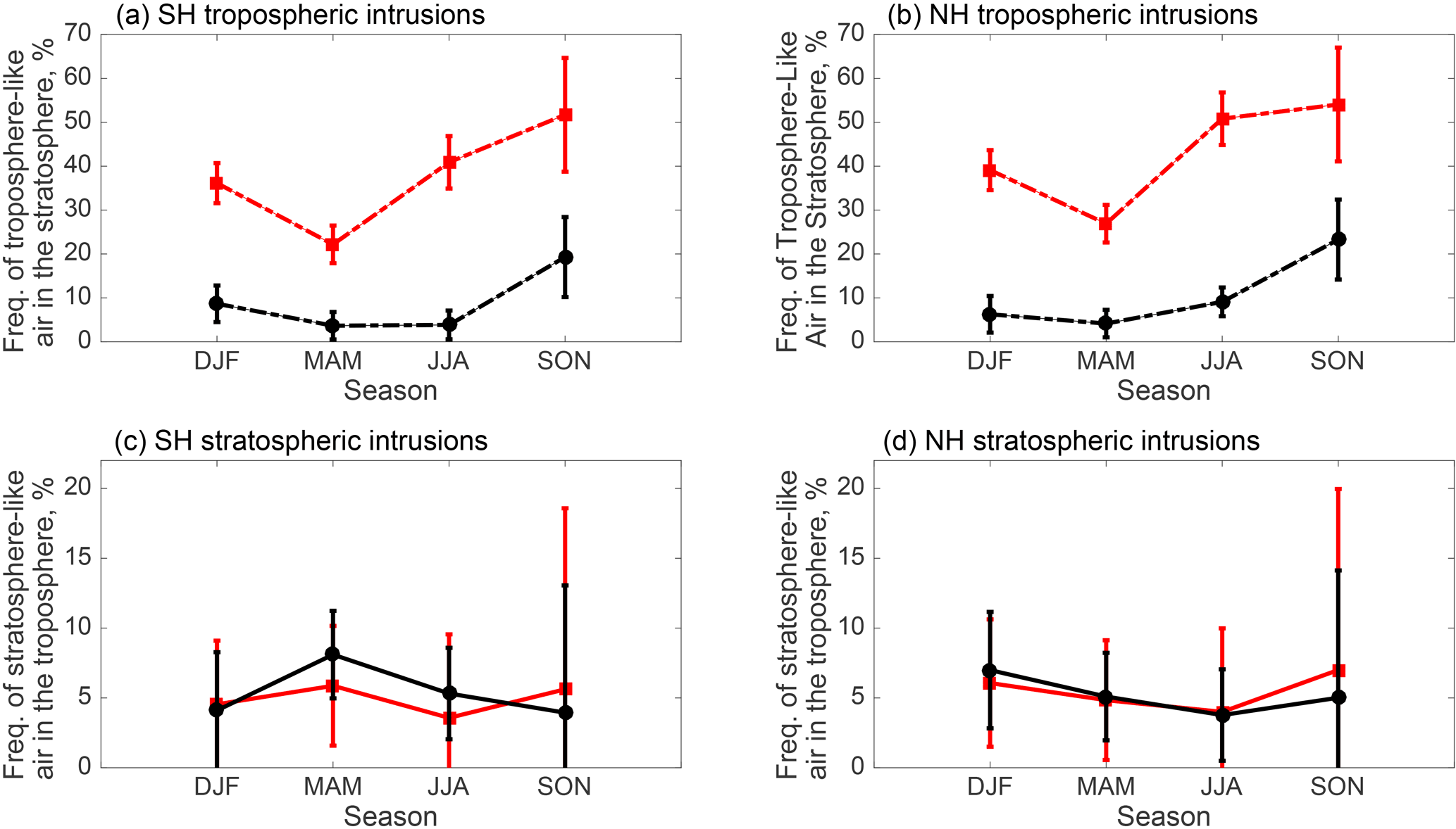
Figure 12A seasonal representation of the intrusions depicted in Fig. 11: (a) tropospheric intrusions in the Southern Hemisphere, (b) tropospheric intrusions in the Northern Hemisphere, (c) stratospheric intrusions in the Southern Hemisphere, and (d) stratospheric intrusions in the Northern Hemisphere. Each season is an average of the extratropical intrusion frequency with error bars indicating 1 standard deviation of the seasonal mean. ACE-FTS intrusions are in red squares and CMAM30HR intrusions are in black circles. Note the seasonality represented may be impacted by the sampling of ACE-FTS and may not representative for the full atmosphere.
A mechanism for extratropical tropospheric air to be uplifted into the stratosphere has been identified recently. Building on the work of Pan et al. (2009), Peevey et al. (2014) showed that the occurrence of double tropopauses is associated with the strength of the tropopause inversion layer (TIL), as well as Rossby wave breaking. They also showed that as the strength of the TIL increases, cyclonic circulation in the upper troposphere switches to anticyclonic circulation, thereby driving an increase in the upward motion. Based on the double tropopause calculations of Schwartz et al. (2015), it is likely that ACE-FTS observes this phenomenon of upward motion, leading to a higher frequency of tropospheric intrusions across the extratropical regions. CMAM30HR appears to inadequately simulate this mechanism since it does not have a sharply defined tropopause compared to reality (Birner and Bönisch, 2011). It is possible that both the spatial and vertical resolutions of the simulations performed limit the model's ability to capture this synoptic-scale activity.
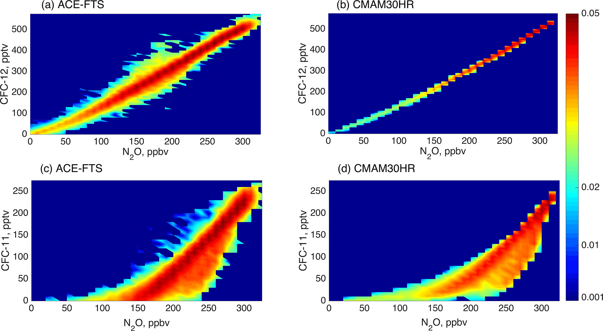
Figure 13JPDFs, as described in the text, of N2O–CFC-12 for (a) ACE-FTS and (b) CMAM30HR, and N2O–CFC-11 for (c) ACE-FTS and (d) CMAM30HR. All stratospheric ACE-FTS observations and subsampled model output in the Northern Hemisphere are included.
Seasonal averages of the tropospheric and stratospheric intrusions are shown in Fig. 12, where Fig. 12a and b are the tropospheric intrusion frequencies for the southern and northern extratropics, respectively, and Fig. 12c and d are the stratospheric intrusion frequencies for each hemisphere. For this case, the data shown in Fig. 11 were averaged seasonally in each hemisphere and the error bars represent the latitudinal variability defined as 1 standard deviation of the mean. Recall that since the intrusion frequencies in Fig. 12 are affected by the sampling pattern of ACE-FTS, the seasonality shown may not be representative of the actual seasonality of the atmosphere. The stratospheric intrusion comparisons are remarkably good; there does not appear to be a significant difference between the simulations and the measurements. Therefore, the differences are primarily due to the finite horizontal and vertical resolution of the model, which leads to differences in the representation of stratosphere–troposphere intrusion events. The comparisons of tropospheric intrusions exhibit similar behaviour between the two hemispheres. The measurement–model differences appear to be largest during JJA and smallest during MAM. The consistency of the increase during SON in tropospheric intrusion frequency between the two hemispheres may be the result of convective overspill into the stratosphere across the subtropical tropopause barrier if the majority of the tropospheric intrusions are driven by convection in the tropics. This convective influence could extend across the extratropical latitudes via isentropic transport from the tropics. The strength of the convection during JJA and SON and its influence on mixing across the tropopause barrier is observed by the largest variability in the stratospheric intrusions.
5.3 The tropical pipe
In this section, JPDFs are used to investigate the tropical pipe barrier. Figure 13 illustrates the N2O–CFC JPDFs of the entire northern hemispheric stratosphere, beginning at 2 km above the tropopause to 30 km (up to 10 hPa), for ACE-FTS (Fig. 13a, c) and CMAM30HR (Fig. 13b, d) for CFC-12 (Fig. 13a, b) and CFC-11 (Fig. 13c, d). Hegglin and Shepherd (2007) have highlighted the use of this technique for comparing CMAM and ACE-FTS measurements. The N2O–CFC-12 JPDFs (Fig. 13a and b) exhibit a quasi-linear relationship in both the measurements and the simulations. The loss rates of CFC-12 and N2O are very similar in the upper troposphere and lower stratosphere, leading to a linear relationship in the JPDFs. The model JPDFs tend to peak at the higher concentrations of N2O and CFC-12 but are more evenly distributed throughout the range of concentrations. These differences between the measurements and simulations are likely due to the overly rapid BDC in the model simulation, leading to higher concentrations of the trace gases in the simulation, which is consistent with the zonal mean comparisons discussed in Sect. 4. The ACE-FTS data in Fig. 13a are much more scattered than the CMAM30HR in Fig. 13b, where the simulated tracers are highly correlated and the JPDF is highly compact. The differences in the spread of the correlations are related to differences in mixing and chemistry but are also influenced by the precision of the ACE-FTS measurements and the constraint of the boundary conditions in the simulations. The CMAM30HR JPDF is very compact because of the similarity of the chemical losses of the two tracers in the model. Additionally, the surface boundary conditions applied do not represent the variability observed in the atmosphere. It is the atmospheric variability that contributes to the variability observed in the ACE-FTS JPDF around 150–200 ppbv of N2O (Hegglin and Shepherd, 2007).
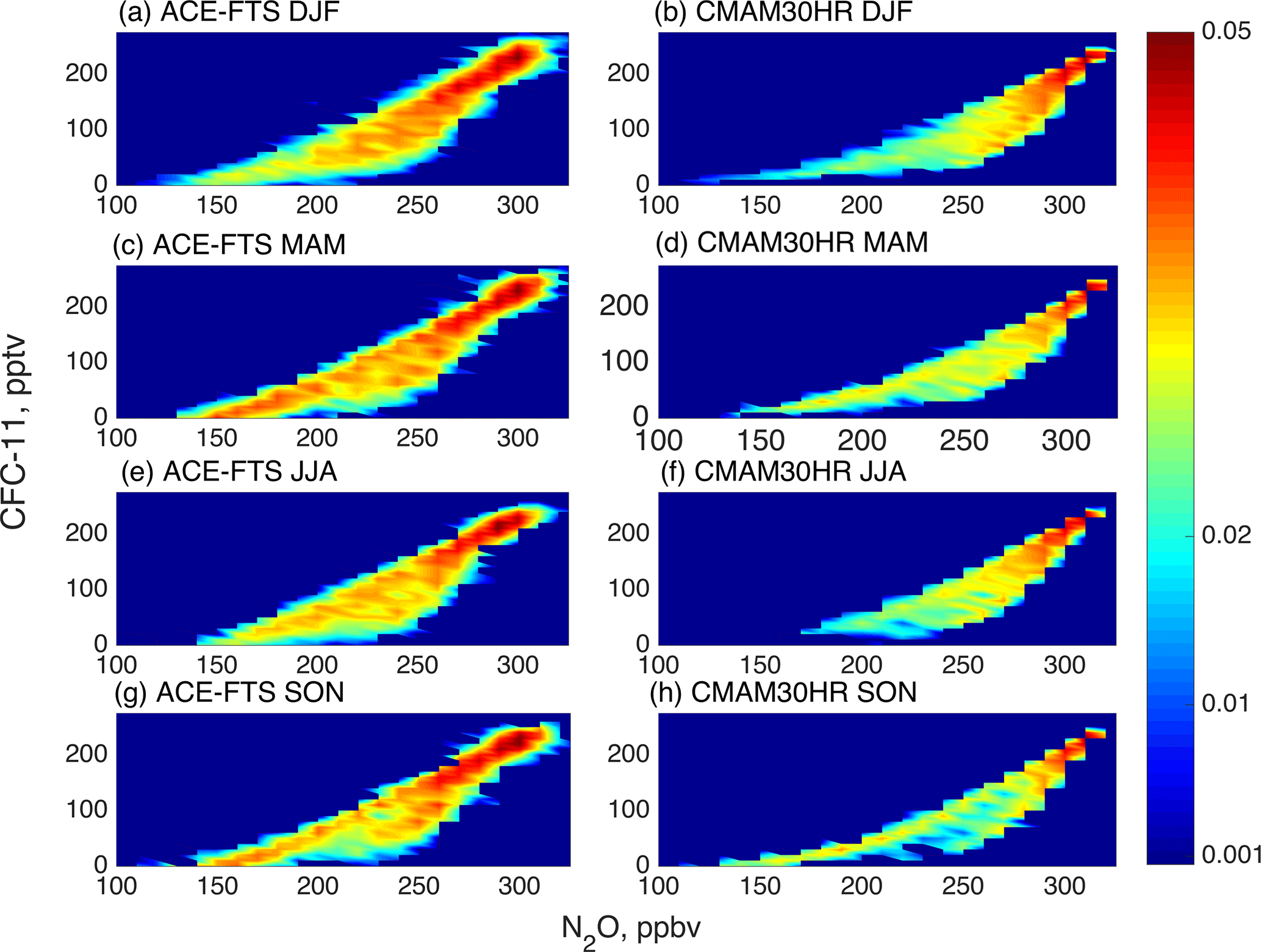
Figure 14Tropical JPDFs of N2O–CFC-11, as described in the text, separated by season. Only stratospheric ACE-FTS observations (left column) and CMAM30HR simulations (right column) within the height-dependent tropical turnaround latitudes have been included.
The N2O–CFC-11 JPDFs show two segments of linear correlations in both the measurements and model results (shown in Fig. 13c and d, respectively) that would have otherwise been overlooked in data-dense tracer–tracer correlation plots (also see Hegglin and Shepherd, 2007). The presence of a bimodal correlation between N2O and CFC-11 has been previously observed by Plumb (1996). The separation is caused by differences in local chemistry in the tropical pipe region. The tropics are somewhat isolated from the midlatitudes so that the steeper slope is a signature of the local chemistry, or the relative loss rates of CFC-11 and N2O in the tropical lower stratosphere. This relationship is observed because the photochemical lifetime of CFC-11 is shorter than the timescale for mixing by horizontal eddy transport timescale (Plumb, 2002). According to Plumb and Ko (1992), slope equilibrium conditions that define the linear relationship seen in the N2O–CFC-12 JPDF are only satisfied if the photochemical lifetime of a species is much greater than the horizontal eddy transport timescale. When this condition is satisfied, the slopes of the isopleths are only a function of atmospheric circulation.
Isolating the measurements and simulations in the tropical region allows for the characteristics of the tropical pipe to be investigated. A JPDF comparison is provided in Fig. 14 for both the ACE-FTS measurements and the CMAM30HR simulations in the tropics during the DJF, MAM, JJA, and SON seasons. The data were selected from the tropical latitude region using estimates of the turnaround latitude, the height-dependent latitude where the tropical upwelling is zero, determined from CMAM30HR monthly mean vertical velocities. Bimodal behaviour is observed in each season and in both the measured and simulated JPDFs. In general, the maximum of the JPDF appears to be positioned towards higher concentrations in the simulation compared to the measurements, where the maximum in the probability tends to extend throughout the shallower segment. As was observed in the N2O–CFC-12 JPDFs in Fig. 13, the probabilities tend to be weighted towards the higher concentrations, implying that there is younger air (of tropospheric origin) in the simulated stratosphere than the measured stratosphere. Of note is that the length and the width of the shallower segment are consistently larger in the measurements. The longer length – extending to low concentrations – indicates the presence of older air not found in the model simulations. The larger width also coincides with the degree of separation between the primary and secondary segment in each season, where the simulated JPDFs appear to have a much greater separation than the measurements. These features are likely dependent on the amount of quasi-horizontal mixing influencing the JPDFs, implying that there is not enough quasi-horizontal mixing occurring in the simulation. However, the differences between the measurements and simulations are primarily in the steepness of this segment of the JPDF, which is an indication of insufficient mixing into the tropics rather than too rapid tropical ascent. If it was just too fast ascent, both tracers would be affected in the same way. But because the midlatitude N2O–CFC-11 relationship is less steep, it is the mixing in of this air that makes the tropics have shallower slope. Then it becomes a question of whether mixing is underestimated because the ascent is too fast or whether the model does not simulate the structure of the pathways of the BDC correctly.
There is an evolution of the characteristics of the JPDFs shown in Fig. 14. During DJF, there is minimal separation between the two segments. The position of the maximum in the JPDF (the red region) in Fig. 14a does not extend below 200 ppbv of N2O, while the location of the maximum of the simulated JPDF in Fig. 14b is limited to above 250 ppbv of N2O with the maximum primarily located above the separation of the two segments. During MAM, the maximum probability of the ACE-FTS JPDF in Fig. 14c extends throughout the shallow and steep segments. This implies that there is significant mixing occurring during this time period. In the simulated MAM, Fig. 14d, the maximum of the probability is restricted to the higher concentrations of N2O, prior to the separation of the two segments. This indicates that while mixing is occurring, it does not occur frequently enough to simulate the atmosphere well.
During JJA, the two segments begin to separate in both the measured and simulated JPDFs. The shallower segment in the simulated JPDF is the shortest during JJA of all the seasons with the maximum of the probability residing at the highest concentrations. This indicates that the upwelling during this season is too strong and it may also be too isolated since there appears to be more mixing in the measured JPDF. During SON, the separation between the segments is most prominent, indicating that this time of year exhibits the least mixing. Based on these comparisons, it is still difficult to discern the relative contributions of the tropical upwelling and quasi-horizontal mixing to the differences in the JPDFs of the model and measurements. To interpret these differences, the results of the TLP model simulations described previously are used. These simulations provide a basis for determining how much the residual circulation needs to slow down within CMAM30HR and what impact that may have on mixing of air between the tropical and extratropical regions.
An analysis of the effects of the strength of the BDC and the mixing in CMAM30HR was achieved through a suite of simulations computed with the TLP to test a range of mean circulation strengths and mixing efficiencies. The TLP runs began with the CMAM30HR best fit to the TLP model and then the best combination was selected to match the ACE-FTS measurement profiles of CFC-11 and CFC-12, as well as an age-of-air estimate derived from balloon-borne measurements (Ray et al., 2016). There were 480 simulations initialized with different combinations of w∗ (velocity of tropical upwelling) and ϵ (the mixing efficiency) settings. The fraction of the CMAM30 w∗ used to initialize the TLP model ranged from 0.20 to 1.24 and the ϵ ranged from 0.18 to 1.50. In each TLP simulation run, the relationship between mean circulation and mixing is constrained by the vertically averaged mixing efficiency (Ray et al., 2016). The mixing efficiency in the TLP model is defined as ϵ = α∕λτ, where α is the ratio of tropical to extratropical mass, λ is the rate of the mean circulation influence, specifically the mass flux out of the tropics due to mean circulation, and τ is the mixing time or timescale for mass flux between the tropics and extratropics (Ray et al., 2014; Garny et al., 2014). Therefore, the mixing efficiency is dependent on both the mean circulation and the horizontal mixing mass flux (Garny et al., 2014). The same suite of TLP model experiments Ray et al. (2016) describe are also used here but the analysis has been modified to investigate the behaviour of the tropical pipe in CMAM30HR in further detail.
Ray et al. (2016) found that the CMAM30HR simulations best match the ACE-FTS measurements when the w∗ is between 0.27 and 0.32 mm s−1 (a reduction from the fitting estimate of 0.4 mm s−1) and ϵ ranges from 0.7 to 1.2 (an increase from the fitting estimate of 0.55). Ray et al. (2016) found that since ϵ is inversely proportional to both λ and τ, there is a compensating effect with changes in w∗ (λ) or τ. For the CMAM30HR changes derived, w∗ needed to be slowed down significantly below 20 km, and above 24 km. For constant ϵ that would result in larger τ (less mixing). However, Ray et al. (2016) found that ϵ also needed to be increased so there needed to be more mixing than would result from slower w∗ and constant τ, but not enough of an increase in ϵ so that the mixing times were less (more mixing) than CMAM30HR has currently. Ray et al. (2016) concluded that with the increase in ϵ, mixing times are reduced but still longer than the current CMAM30HR mixing times.
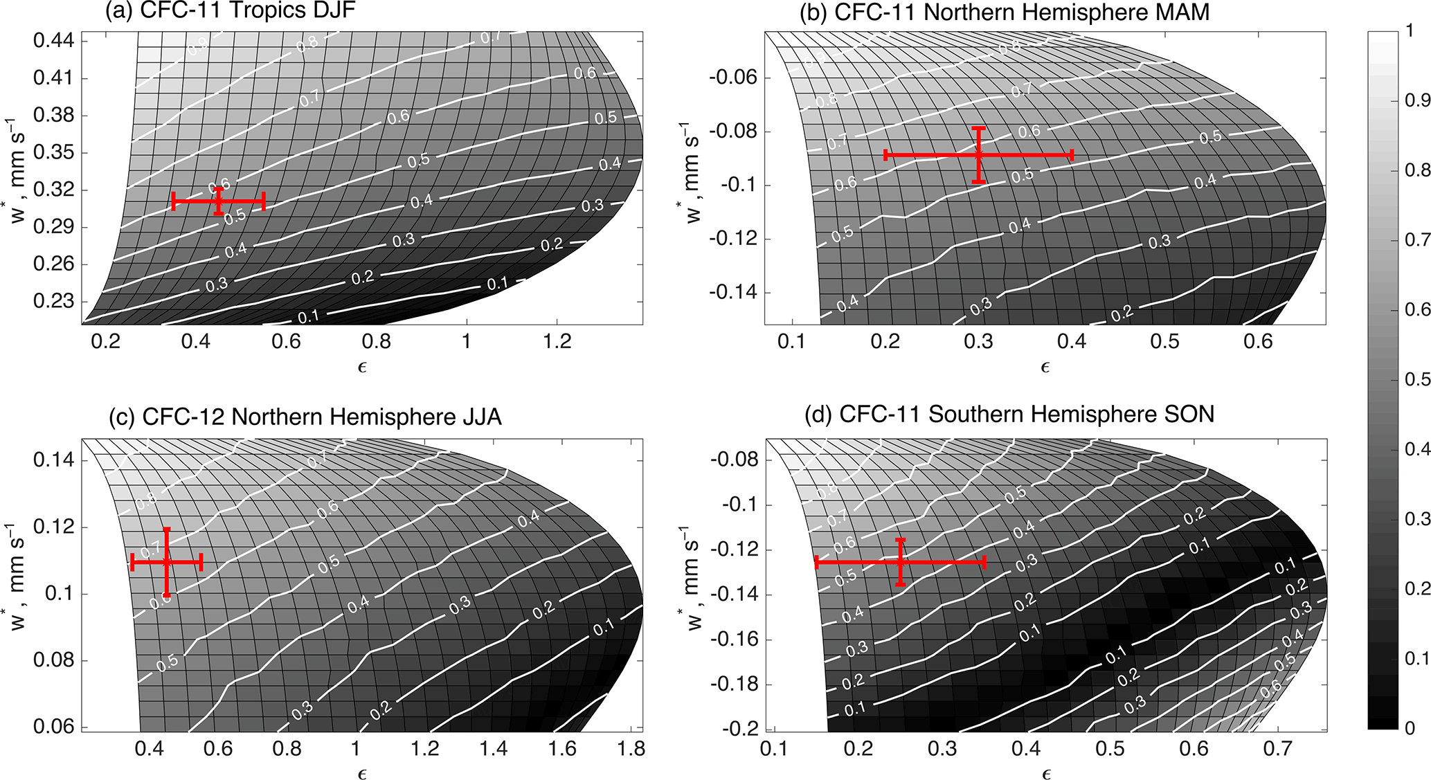
Figure 15Examples of the TLP comparisons described in the text. The grey scale on each panel indicates the comparison between ACE-FTS and the TLP simulations over various w∗ (y axes) and ϵ cases (x axes). The white lines identify the agreement with ACE-FTS (grey colour scale). The red marker indicates the CMAM30HR estimated values of w∗ and ϵ. The examples shown are (a) CFC-11 tropics during the DJF season, (b) CFC-11 Northern Hemisphere during the MAM season, (c) CFC-12 Northern Hemisphere during the JJA season, and (d) CFC-11 Southern Hemisphere during the SON season.
In this study, the TLP simulations are used in a spatial and seasonal context to determine the changes required in the CMAM30HR simulations to match the ACE-FTS observations. The three regions investigated (the tropics and the northern and southern extratropics) were defined by the turnaround latitude of the tropical upwelling and by exclusion of the polar vortex in each hemisphere using a 1.2 × 10⁻⁴ s−1 scaled potential vorticity threshold (e.g. Manney et al., 2007). The vortex is excluded in these comparisons because the TLP model does not simulate its complexity. For each of the 480 simulations of the TLP model and the ACE-FTS measurements, profiles for CFC-11 and CFC-12 were averaged over 16–27 km in the extratropics and 16–29 km in the tropics. To capture the monthly coverage of the ACE-FTS measurements, a weighting function for each region and season was applied based on the relative contribution of the occultations observed in each month of the particular season and region (the tropics and northern/southern extratropics). The vertically averaged and monthly weighted measurements were compared to the individual simulations of the TLP model that represent varying levels of tropical upwelling and mixing efficiencies. For each of the comparisons, the absolute value of the differences is used and scaled to the maximum of the range of all differences so that each of the scales range from zero to one.
Figure 15 shows four examples of these comparisons plotted by the seasonally averaged, regionally specific modelled values of mixing, ϵ, and upwelling, w∗, for each simulation. The x-axis and y-axis values do not represent the setting used to run the simulation – they are the values simulated by the TLP model and lead to the curvature seen in the plots. The shading of each plot indicates the level of agreement, where the darker regions indicate the minimum differences between ACE-FTS and the TLP simulations. The white-to-black shading is reinforced by white contours of the same quantity to illustrate the comparison more clearly. The relative CMAM30HR position is shown by the red marker and the error bars represent the estimated range of uncertainty based on the optimization exercise with the TLP model. These comparisons all indicate that the CMAM30HR values of ϵ and w∗ would require some change to bring the simulations closer to agreement with the ACE-FTS measurements (i.e. bringing the red marker towards the dark shaded region). The dependence of w∗ on ϵ and vice versa is not the same across regions and seasons for either CFC-11 or CFC-12. There are often limited ranges in which agreement between the TLP simulations and ACE-FTS can be assessed but it is clear that changes could lead to improvements in the agreement (such as in Fig. 15b). There are some scenarios where the mixing is required to change much more than the tropical upwelling (see Fig. 15c for an example) or where there can be a range of mixing efficiency and upwelling values that lead to better agreement (as in Fig. 15d).
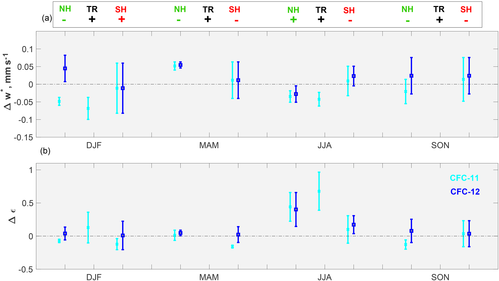
Figure 16A summary of the TLP comparisons by season and region: panel (a) indicates the changes required in tropical upwelling, w∗, while panel (b) indicates the changes in the mixing, ϵ, required for the CMAM30HR simulation to agree with the ACE-FTS observations. The “−” and “+” symbols at the top of the figure indicate the direction of mass transport (downwelling or upwelling, respectively) for each season and region (green for Northern Hemisphere, black for tropics, and red for the Southern Hemisphere). The changes required based on CFC-11 are shown in cyan and the changes required based on CFC-12 are shown in blue.
The changes that would bring CMAM30HR into agreement with ACE-FTS based on the TLP simulation comparisons for CFC-11 and CFC-12 have been calculated. This was done by finding where the differences between ACE-FTS and the TLP simulation are below a certain threshold (0.2 for all regions and seasons) and determining the ranges of w∗ and ϵ over which this occurs. The average values (cyan “x” markers for CFC-11 and blue square markers for CFC-12) and ranges (error bars) of the changes to w∗ and ϵ calculated are shown in Fig. 16. The changes in w∗ were calculated based on the absolute value of w∗ so that the interpretation of the differences calculated was not dependent on the sign of w∗. This means that a positive change is always an acceleration of the BDC, even when w∗ is typically negative, such as in the extratropics. Figure 16a shows these changes for each region and across the four seasons. The sign of w∗ values is indicated above Fig. 16a, where the green symbols are for the northern hemispheric extratropics, the black symbols are for the tropics, and the red symbols are for the southern hemispheric extratropics. In some cases, the agreement between ACE-FTS and the TLP simulations did not meet the 0.2 threshold so there is no result available for Fig. 16.
The changes required to w∗ in the tropical region are significant in the CFC-11 comparisons in two seasons, DJF and JJA, indicating that the w∗ strength should be reduced by 0.05 to 0.10 mm s−1 in DJF and by 0.03 to 0.12 mm s−1 in JJA. The lack of a significant change during MAM and SON indicates that there is no argument for changes to the tropical upwelling in CMAM30HR. The Southern Hemisphere w∗ changes are not significantly different from zero during any season, suggesting that changes in the w∗ in this region would not improve the comparisons. However, there are significant changes identified in three of the four seasons in the extratropical region of the Northern Hemisphere. In DJF, an increase in w∗ is required in the Northern Hemisphere by the CFC-12 comparisons, implying that strength of the downwelling during this season should increase by up to 0.08 mm s−1. However, the CFC-11 comparisons indicate that w∗ should decrease by approximately 0.05 mm s−1. This contradiction necessitates the conclusion that no change is recommended in w∗ in the northern hemispheric extratropical region during DJF. During MAM in the Northern Hemisphere, CFC-11 and CFC-12 comparisons suggest an increase in the downwelling by approximately 0.05 mm s−1. By summer in the Northern Hemisphere (JJA), the tropical pipe has shifted poleward such that the northern hemispheric extratropical w∗ values are positive and require a decrease in value as compared to the measurements. While this season tends to have the most active tropical upwelling, these results suggest that the upwelling in CMAM30HR may be too rapid or, since the southern extratropics appear to have increased downwelling during JJA, may be displaced in latitude.
The calculations of changes to the mixing parameter, ϵ, shown in Fig. 16b, indicate that changes could be made in the tropics and extratropics differently across the seasons. The results indicate, based on CFC-11 and CFC-12 comparisons, that mixing efficiency in the tropics and in the northern hemispheric extratropics needs to increase during JJA. Based on the CFC-12 comparison, mixing efficiency in the southern hemispheric extratropics should also be increased during JJA. Significant changes are indicated from the CFC-11 comparisons for the remaining seasons in the extratropical regions. In the Northern Hemisphere and Southern Hemisphere during DJF, decreased mixing efficiency is suggested. During MAM, CFC-12 indicates there may be an increase suggested but the result is not supported by CFC-11 comparisons. In the Southern Hemisphere, CFC-11 comparisons show that a decrease in mixing efficiency is necessary. During SON, CFC-11 comparisons also indicate a decrease in mixing efficiency in the Northern Hemisphere only. Generally, in all seasons except JJA, mixing efficiency in the extratropics is suggested to decrease.
Combining the ϵ parameter results with the decrease in w∗ suggested in Fig. 16a, an increase in mixing timescales between the tropics and northern hemispheric extratropics is required during JJA. It follows that if w∗ needs to be reduced in the model then a reduction in wave activity is required. The specific waves that break in the lower, middle, and upper stratosphere that could be investigated for possible sources of increased w∗. For mixing changes, the background state of the winds and corresponding critical layers for wave breaking could be investigated for critical layers that extend too far into the tropics.
In this work, ACE-FTS measurements of CFC-11, CFC-12, and N2O have been used to assess the CMAM30HR simulations of these tracers and, thereby, indirectly the transport processes in the lower stratosphere in the model. By treating each tracer in the specified dynamics simulation explicitly, the CMAM30HR run allows for the direct comparison of the measurements to model output. The advanced sampling technique employed here allows for detailed interpretation of the comparisons. Of the species investigated, it was found that CMAM30HR consistently overpredicts tracer concentrations in the lower to mid-stratosphere. The largest and most widespread overpredictions occur in the northern hemispheric winter and spring, when the BDC is most active in that hemisphere.
The investigation of simulated mixing barriers identified a number of issues in the CMAM30HR simulations. The polar vortex comparisons reveal issues in both the timing and strength of the downwelling portion of the deep branch, which is related to the too-rapid BDC in CMAM30 simulations observed in the zonal mean comparisons. The extratropical tropopause barrier in the model appears to represent stratospheric intrusion events well, as evidenced by Fig. 12c and d. However, tropospheric intrusions are poorly simulated in most seasons (Fig. 12a and b), with the largest discrepancies occurring during JJA in both hemispheres. The tropical pipe mixing barrier analysis suggests that while the strength of the simulated BDC (i.e. upwelling in the tropics and downwelling in the extratropics) may partially explain the too young air found in the mid-stratosphere, mixing efficiency may play at least as prominent a role and seems to be underestimated, particularly in the JJA season in all regions.
The analysis presented here highlights the importance of scrutinizing the mixing efficiency in CCMs and GCMs since it may be related to the mechanisms driving the projected trends in stratospheric circulation, thereby influencing the simulations of stratospheric ozone recovery and climate change. The techniques used in this work, including the advanced sampling and use of the tropical leaky pipe model, have proven illuminating. It is suggested that other CCMs and GCMs investigate the use of these techniques in future studies.
The ACE-FTS Level 2 data used in this study can be obtained via the ACE-FTS website (registration required, http://www.ace.uwaterloo.ca). The HATS combined CFC data can be acquired via NOAA's ftp site, ftp://ftp.cmdl.noaa.gov/hats/cfcs/. The CMAM30 data set can be downloaded via Environment and Climate Change Canada's climate modelling website, http://climate-modelling.canada.ca/climatemodeldata/cmam/output/. Additional fields specific to the CMAM30HR simulation are available available from David Plummer (david.plummer@canada.ca). The TLP data are available from Eric Ray (eric.ray@noaa.gov).
The authors declare that they have no conflict of interest.
This project was funded by grants from the Canadian Space Agency (CSA) and
the Natural Sciences and Engineering Research Council of Canada (NSERC). The
Atmospheric Chemistry Experiment (ACE), also known as SCISAT, is a
Canadian-led mission mainly supported by the CSA and the NSERC. The
development of the CMAM30 data set was funded by the CSA. We thank Peter Bernath for his leadership of the ACE mission. We also thank Ted Shepherd,
Dylan Jones, and John Scinocca for their leadership and support of the CMAM30
Project. The HATS measurements were funded in part by the Atmospheric
Chemistry Project of the National Oceanographic and Atmospheric
Administration (NOAA) Climate and Global Change Program. The authors thank
Geoff Dutton, Debra Mondeel, and Steve Montzka for their work on measurements
of these important trace gases in the HATS program. The authors also thank
the anonymous reviewers, Matthew Toohey, and Chris McLinden for their
extensive and thoughtful feedback on this paper.
Edited by: Martin Dameris
Reviewed by: Matthew Toohey and two anonymous referees
Abalos, M., Legras, B., Ploeger, F., and Randel, W. J.: Evaluating the advective Brewer-Dobson circulation in three reanalyses for the period 1979–2012, J. Geophys. Res., 120, 7534–7554, 2015. a
Abrams, M. C., Manney, G. L., Gunson, M. R., Abbas, M. M., Chang, A. Y., Goldman, A., Irion, F. W., Michelsen, H. A., Newchurch, M. J., Rinsland, C. P., Salawitch, R. J., Stiller, G. P., and Zander, R.: Trace gas transport in the Arctic Vortex inferred from ATMOS ATLAS-2 observations during April 1993, Geophys. Res. Lett., 23, 2345–2348, https://doi.org/10.1029/96GL00704, 1996a. a
Abrams, M. C., Manney, G. L., Gunson, M. R., Abbas, M. M., Chang, A. Y., Goldman, A., Irion, F. W., Michelsen, H. A., Newchurch, M. J., Rinsland, C. P., Salawitch, R. J., Stiller, G. P., and Zander, R.: ATMOS/ATLAS3 observations of long-lived tracers and descent in the Antarctic Vortex in November 1994, Geophys. Res. Lett., 23, 2341–2344, https://doi.org/10.1029/96GL00705, 1996b. a
Allen, D. R., Stanford, J. L., Nakamura, N., López Valverde, M. A., López-Puertas, M., Taylor, F. W., and Remedios, J. J.: Antarctic polar descent and planetary wave activity observed in ISAMS CO from April to July 1992, Geophys. Res. Lett., 27, 665–668, https://doi.org/10.1029/1999GL010888, 2000. a
Allen, N. D. C., Bernath, P. F., Boone, C. D., Chipperfield, M. P., Fu, D., Manney, G. L., Oram, D. E., Toon, G. C., and Weisenstein, D. K.: Global carbon tetrachloride distributions obtained from the Atmospheric Chemistry Experiment (ACE), Atmos. Chem. Phys., 9, 7449–7459, https://doi.org/10.5194/acp-9-7449-2009, 2009. a, b
Austin, J., Shindell, D., Beagley, S. R., Brühl, C., Dameris, M., Manzini, E., Nagashima, T., Newman, P., Pawson, S., Pitari, G., Rozanov, E., Schnadt, C., and Shepherd, T. G.: Uncertainties and assessments of chemistry-climate models of the stratosphere, Atmos. Chem. Phys., 3, 1–27, https://doi.org/10.5194/acp-3-1-2003, 2003. a
Beagley, S. R., de Grandpré, J., Koshyk, J. N., McFarlane, N. A., and Shepherd, T. G.: Radiative-dynamical climatology of the first-generation Canadian middle atmosphere model, Atmos. Ocean, 35, 293–331, https://doi.org/10.1080/07055900.1997.9649595, 1997. a
Bernath, P. F.: The Atmospheric Chemistry Experiment (ACE), J. Quant. Spectrosc. Ra., 186, 3–16, https://doi.org/10.1016/j.jqsrt.2016.04.006, 2017. a
Bernath, P. F., McElroy, C. T., Abrams, M. C., Boone, C. D., Butler, M., Camy-Peyret, C., Carleer, M., Clerbaux, C., Coheur, P. F., Colin, R., DeCola, P., DeMazière, M., Drummond, J. R., Dufour, D., Evans, W. F. J., Fast, H., Fussen, D., Gilbert, K., Jennings, D. E., Llewellyn, E. J., Lowe, R. P., Mahieu, E., McConnell, J. C., McHugh, M., McLeod, S. D., Michaud, R., Midwinter, C., Nassar, R., Nichitiu, F., Nowlan, C., Rinsland, C. P., Rochon, Y. J., Rowlands, N., Semeniuk, K., Simon, P., Skelton, R., Sloan, J. J., Soucy, M. A., Strong, K., Tremblay, P., Turnbull, D., Walker, K. A., Walkty, I., Wardle, D. A., Wehrle, V., Zander, R., and Zou, J.: Atmospheric Chemistry Experiment (ACE): Mission overview, Geophys. Res. Lett., 32, L15S01, https://doi.org/10.1029/2005GL022386, 2005. a, b, c
Birner, T. and Bönisch, H.: Residual circulation trajectories and transit times into the extratropical lowermost stratosphere, Atmos. Chem. Phys., 11, 817–827, https://doi.org/10.5194/acp-11-817-2011, 2011. a, b
Boone, C. D., Nassar, R., Walker, K. A., Rochon, Y., McLeod, S. D., Rinsland, C. P., and Bernath, P. F.: Retrievals for the atmospheric chemistry experiment Fourier-transform spectrometer, Appl. Optics, 44, 7218–7231, https://doi.org/10.1364/AO.44.007218, 2005. a, b, c, d
Boone, C. D., Walker, K. A., and Bernath, P. F.: Version 3 retrievals for the atmospheric chemistry experiment Fourier transform spectrometer (ACE-FTS), The Atmospheric Chemistry Experiment ACE at 10: A Solar Occultation Anthology, A. Deepak Publishing, Hampton, Va., USA, 2013. a, b, c, d
Brewer, A. W.: Evidence for a world circulation provided by the measurements of helium and water vapour distribution in the stratosphere, Q. J. Roy. Meteor. Soc., 75, 351–363, https://doi.org/10.1002/qj.49707532603, 1949. a
Brown, A. T., Chipperfield, M. P., Boone, C., Wilson, C., Walker, K. A., and Bernath, P. F.: Trends in atmospheric halogen containing gases since 2004, J. Quant. Spectrosc. Ra., 112, 2552–2566, https://doi.org/10.1016/j.jqsrt.2011.07.005, 2011. a
Brown, A. T., Volk, C. M., Schoeberl, M. R., Boone, C. D., and Bernath, P. F.: Stratospheric lifetimes of CFC-12, CCl4, CH4, CH3Cl and N2O from measurements made by the Atmospheric Chemistry Experiment-Fourier Transform Spectrometer (ACE-FTS), Atmos. Chem. Phys., 13, 6921–6950, https://doi.org/10.5194/acp-13-6921-2013, 2013. a
Brown, A. T., Chipperfield, M. P., Richards, N. A. D., Boone, C., and Bernath, P. F.: Global stratospheric fluorine inventory for 2004–2009 from Atmospheric Chemistry Experiment Fourier Transform Spectrometer (ACE-FTS) measurements and SLIMCAT model simulations, Atmos. Chem. Phys., 14, 267–282, https://doi.org/10.5194/acp-14-267-2014, 2014. a
Butchart, N.: The Brewer-Dobson circulation, Rev. Geophys., 52, 157–184, https://doi.org/10.1002/2013RG000448, 2014. a, b, c, d, e, f, g, h, i
Dee, D. P., Uppala, S. M., Simmons, A. J., Berrisford, P., Poli, P., Kobayashi, S., Andrae, U., Balmaseda, M. A., Balsamo, G., Bauer, P., Bechtold, P., Beljaars, A. C. M., van de Berg, L., Bidlot, J., Bormann, N., Delsol, C., Dragani, R., Fuentes, M., Geer, A. J., Haimberger, L., Healy, S. B., Hersbach, H., Hólm, E. V., Isaksen, L., Kållberg, P., Köhler, M., Matricardi, M., McNally, A. P., Monge Sanz, B. M., Morcrette, J. J., Park, B. K., Peubey, C., de Rosnay, P., Tavolato, C., Thépaut, J. N., and Vitart, F.: The ERA-Interim reanalysis: configuration and performance of the data assimilation system, Q. J. Roy. Meteorol. Soc., 137, 553–597, https://doi.org/10.1002/qj.828, 2011. a
deGrandpré, J., Beagley, S. R., Fomichev, V. I., Griffioen, E., McConnell, J. C., Medvedev, A. S., and Shepherd, T. G.: Ozone climatology using interactive chemistry: Results from the Canadian Middle Atmosphere Model, J. Geophys. Res., 105, 26475–26491, https://doi.org/10.1029/2000JD900427, 2000. a
Diallo, M., Legras, B., and Chédin, A.: Age of stratospheric air in the ERA-Interim, Atmos. Chem. Phys., 12, 12133–12154, https://doi.org/10.5194/acp-12-12133-2012, 2012. a
Dickinson, R. E.: Vertical propagation of planetary rossby waves through an atmosphere with Newtonian cooling, J. Geophys. Res., 74, 929–938, https://doi.org/10.1029/JB074i004p00929, 1969. a
Dobson, G. M. B.: Origin and Distribution of the Polyatomic Molecules in the Atmosphere, P. Roy. Soc. A-Math. Phy., 236, 187–193, https://doi.org/10.1098/rspa.1956.0127, 1956. a
Dobson, G. M. B., Harrison, D. N., and Lawrence, J.: Measurements of the Amount of Ozone in the Earth's Atmosphere and Its Relation to Other Geophysical Conditions. Part III, P. Roy. Soc. A-Math. Phy., 122, 456–486, https://doi.org/10.1098/rspa.1929.0034, 1929. a
Elkins, J. W., Thompson, T. M., Swanson, T. H., Butler, J. H., Hall, B. D., Cummings, S. O., Fisher, D. A., and Raffo, A. G.: Decrease in the growth rates of atmospheric chlorofluorocarbons 11 and 12, Nature, 364, 780–783, https://doi.org/10.1038/364780a0, 1993. a
Engel, A., Möbius, T., Bönisch, H., Schmidt, U., Heinz, R., Levin, I., Atlas, E., Aoki, S., Nakazawa, T., Sugawara, S., Moore, F., Hurst, D., Elkins, J., Schauffler, S., Andrews, A., and Boering, K.: Age of stratospheric air unchanged within uncertainties over the past 30 years, Nat. Geosci., 2, 28–31, https://doi.org/10.1038/NGEO388, 2009. a, b, c
Eyring, V., Harris, N. R. P., Rex, M., Shepherd, T. G., Fahey, D. W., Amanatidis, G. T., Austin, J., Chipperfield, M. P., Dameris, M., Forster, P. M. D. F., Gettelman, A., Graf, H. F., Nagashima, T., Newman, P. A., Pawson, S., Prather, M. J., Pyle, J. A., Salawitch, R. J., Santer, B. D., and Waugh, D. W.: A Strategy for Process-Oriented Validation of Coupled Chemistry-Climate Models, B. Am. Meteorol. Soc., 86, 1117–1133, https://doi.org/10.1175/BAMS-86-8-1117, 2005. a
Funke, B., García-Comas, M., López-Puertas, M., Glatthor, N., Stiller, G. P., von Clarmann, T., Semeniuk, K., and McConnell, J. C.: Enhancement of N2O during the October–November 2003 solar proton events, Atmos. Chem. Phys., 8, 3805–3815, https://doi.org/10.5194/acp-8-3805-2008, 2008a. a
Funke, B., López-Puertas, M., Garcia-Comas, M., Stiller, G. P., von Clarmann, T., and Glatthor, N.: Mesospheric N2O enhancements as observed by MIPAS on Envisat during the polar winters in 2002–2004, Atmos. Chem. Phys., 8, 5787–5800, https://doi.org/10.5194/acp-8-5787-2008, 2008b. a
Garny, H., Birner, T., Bönisch, H., and Bunzel, F.: The effects of mixing on age of air, J. Geophys. Res., 119, 7015–7034, https://doi.org/10.1002/2013JD021417, 2014. a, b
Gerber, E. P.: Stratospheric versus Tropospheric Control of the Strength and Structure of the Brewer-Dobson Circulation, J. Atmos. Sci., 69, 2857–2877, https://doi.org/10.1175/JAS-D-11-0341.1, 2012. a
Greenblatt, J. B.: Correction to “Tracer-based determination of vortex descent in the 1999/2000 Arctic winter” by J. B. Greenblatt et al., J. Geophys. Res., 107, SOL 50-1–SOL 50-2 , https://doi.org/10.1029/2002JD001597, 2003. a
Greenblatt, J. B., Jost, H. J., Loewenstein, M., Podolske, J. R., Hurst, D. F., Elkins, J. W., Schauffler, S. M., Atlas, E. L., Herman, R. L., Webster, C. R., Bui, T. P., Moore, F. L., Ray, E. A., Oltmans, S., Vömel, H., Blavier, J. F., Sen, B., Stachnik, R. A., Toon, G. C., Engel, A., Müller, M., Schmidt, U., Bremer, H., Pierce, R. B., Sinnhuber, B. M., Chipperfield, M., and Lefèvre, F.: Tracer-based determination of vortex descent in the 1999/2000 Arctic winter, J. Geophys. Res., 107, SOL 22-1–SOL 22-21, https://doi.org/10.1029/2001JD000937, 2002. a
Haenel, F. J., Stiller, G. P., von Clarmann, T., Funke, B., Eckert, E., Glatthor, N., Grabowski, U., Kellmann, S., Kiefer, M., Linden, A., and Reddmann, T.: Reassessment of MIPAS age of air trends and variability, Atmos. Chem. Phys., 15, 13161–13176, https://doi.org/10.5194/acp-15-13161-2015, 2015. a
Hall, T. M. and Plumb, R. A.: Age as a diagnostic of stratospheric transport, J. Geophys. Res., 99, 1059–1070, https://doi.org/10.1029/93JD03192, 1994. a
Hall, T. M. and Waugh, D. W.: Stratospheric residence time and its relationship to mean age, J. Geophys. Res., 105, 6773–6782, https://doi.org/10.1029/1999JD901096, 2000. a
Hardiman, S. C., Lin, P., Scaife, A. A., Dunstone, N. J., and Ren, H.-L.: The influence of dynamical variability on the observed Brewer-Dobson circulation trend, Geophys. Res. Lett., 44, 2885–2892, https://doi.org/10.1002/2017GL072706, 2017. a, b
Haynes, P. and Shuckburgh, E.: Effective diffusivity as a diagnostic of atmospheric transport: 2. Troposphere and lower stratosphere, J. Geophys. Res., 105, 22795–22810, https://doi.org/10.1029/2000JD900092, 2000. a
Hegglin, M. I. and Shepherd, T. G.: O3-N2O correlations from the Atmospheric Chemistry Experiment: Revisiting a diagnostic of transport and chemistry in the stratosphere, J. Geophys. Res., 112, D19301, https://doi.org/10.1029/2006JD008281, 2007. a, b, c, d, e, f, g, h, i
Hegglin, M. I., Boone, C. D., Manney, G. L., Shepherd, T. G., Walker, K. A., Bernath, P. F., Daffer, W. H., Hoor, P., and Schiller, C.: Validation of ACE-FTS satellite data in the upper troposphere/lower stratosphere (UTLS) using non-coincident measurements, Atmos. Chem. Phys., 8, 1483–1499, https://doi.org/10.5194/acp-8-1483-2008, 2008. a
Hegglin, M. I., Boone, C. D., Manney, G. L., and Walker, K. A.: A global view of the extratropical tropopause transition layer from Atmospheric Chemistry Experiment Fourier Transform Spectrometer O3, H2O, and CO, J. Geophys. Res., 114, D00B11, https://doi.org/10.1029/2008JD009984, 2009. a, b
Hegglin, M. I., Tegtmeier, S., Anderson, J., Froidevaux, L., Fuller, R., Funke, B., Jones, A., Lingenfelser, G., Lumpe, J., Pendlebury, D., Remsberg, E., Rozanov, A., Toohey, M., Urban, J., von Clarmann, T., Walker, K. A., Wang, R., and Weigel, K.: SPARC Data Initiative: Comparison of water vapor climatologies from international satellite limb sounders, J. Geophys. Res., 118, 11824–11846, https://doi.org/10.1002/jgrd.50752, 2013. a
Hegglin, M. I., Plummer, D. A., Shepherd, T. G., Scinocca, J. F., Anderson, J., Froidevaux, L., Funke, B., Hurst, D., Rozanov, A., Urban, J., von Clarmann, T., Walker, K. A., Wang, H. J., Tegtmeier, S., and Weigel, K.: Vertical structure of stratospheric water vapour trends derived from merged satellite data, Nat. Geosci., 7, 768–776, https://doi.org/10.1038/NGEO2236, 2014. a, b, c, d
Hoffmann, L., Hoppe, C. M., Müller, R., Dutton, G. S., Gille, J. C., Griessbach, S., Jones, A., Meyer, C. I., Spang, R., Volk, C. M., and Walker, K. A.: Stratospheric lifetime ratio of CFC-11 and CFC-12 from satellite and model climatologies, Atmos. Chem. Phys., 14, 12479–12497, https://doi.org/10.5194/acp-14-12479-2014, 2014. a
Holton, J. R., Haynes, P. H., McIntyre, M. E., Douglass, A. R., Rood, R. B., and Pfister, L.: Stratosphere-troposphere exchange, Rev. Geophys., 33, 403–439, https://doi.org/10.1029/95RG02097, 1995. a
Jin, J. J., Semeniuk, K., Jonsson, A. I., Beagley, S. R., McConnell, J. C., Boone, C. D., Walker, K. A., Bernath, P. F., Rinsland, C. P., Dupuy, E., Ricaud, P., De La Noë, J., Urban, J., and Murtagh, D.: Co-located ACE-FTS and Odin/SMR stratospheric-mesospheric CO 2004 measurements and comparison with a GCM, Geophys. Res. Lett., 32, L15S03, https://doi.org/10.1029/2005GL022433, 2005. a
Jones, A., Walker, K. A., Jin, J. J., Taylor, J. R., Boone, C. D., Bernath, P. F., Brohede, S., Manney, G. L., McLeod, S., Hughes, R., and Daffer, W. H.: Technical Note: A trace gas climatology derived from the Atmospheric Chemistry Experiment Fourier Transform Spectrometer (ACE-FTS) data set, Atmos. Chem. Phys., 12, 5207–5220, https://doi.org/10.5194/acp-12-5207-2012, 2012. a
Jonsson, A. I., de Grandpré, J., Fomichev, V. I., McConnell, J. C., and Beagley, S. R.: Doubled CO2-induced cooling in the middle atmosphere: Photochemical analysis of the ozone radiative feedback, J. Geophys. Res., 109, D24103, https://doi.org/10.1029/2004JD005093, 2004. a
Kawamoto, N. and Shiotani, M.: Interannual variability of the vertical descent rate in the Antarctic polar vortex, J. Geophys. Res., 105, 11935–11946, https://doi.org/10.1029/2000JD900076, 2000. a
Koo, J.-H., Walker, K. A., Jones, A., Sheese, P. E., Boone, C. D., Bernath, P. F., and Manney, G. L.: Global climatology based on the ACE-FTS version 3.5 dataset: Addition of mesospheric levels and carbon-containing species in the UTLS, J. Quant. Spectrosc. Ra., 186, 52–62, https://doi.org/10.1016/j.jqsrt.2016.07.003, 2017. a
Lin, P. and Fu, Q.: Changes in various branches of the Brewer-Dobson circulation from an ensemble of chemistry climate models, J. Geophys. Res., 118, 73–84, https://doi.org/10.1029/2012JD018813, 2013. a, b, c
Mahieu, E., Duchatelet, P., Demoulin, P., Walker, K. A., Dupuy, E., Froidevaux, L., Randall, C., Catoire, V., Strong, K., Boone, C. D., Bernath, P. F., Blavier, J.-F., Blumenstock, T., Coffey, M., De Mazière, M., Griffith, D., Hannigan, J., Hase, F., Jones, N., Jucks, K. W., Kagawa, A., Kasai, Y., Mebarki, Y., Mikuteit, S., Nassar, R., Notholt, J., Rinsland, C. P., Robert, C., Schrems, O., Senten, C., Smale, D., Taylor, J., Tétard, C., Toon, G. C., Warneke, T., Wood, S. W., Zander, R., and Servais, C.: Validation of ACE-FTS v2.2 measurements of HCl, HF, CCl3F and CCl2F2 using space-, balloon- and ground-based instrument observations, Atmos. Chem. Phys., 8, 6199–6221, https://doi.org/10.5194/acp-8-6199-2008, 2008. a, b
Manney, G. L., Daffer, W. H., Zawodny, J. M., Bernath, P. F., Hoppel, K. W., Walker, K. A., Knosp, B. W., Boone, C., Remsberg, E. E., Santee, M. L., Harvey, V. L., Pawson, S., Jackson, D. R., Deaver, L., McElroy, C. T., McLinden, C. A., Drummond, J. R., Pumphrey, H. C., Lambert, A., Schwartz, M. J., Froidevaux, L., McLeod, S., Takacs, L. L., Suarez, M. J., Trepte, C. R., Cuddy, D. C., Livesey, N. J., Harwood, R. S., and Waters, J. W.: Solar occultation satellite data and derived meteorological products: Sampling issues and comparisons with Aura Microwave Limb Sounder, J. Geophys. Res., 112, D24S50, https://doi.org/10.1029/2007JD008709, 2007. a, b, c
Manney, G. L., Harwood, R. S., MacKenzie, I. A., Minschwaner, K., Allen, D. R., Santee, M. L., Walker, K. A., Hegglin, M. I., Lambert, A., Pumphrey, H. C., Bernath, P. F., Boone, C. D., Schwartz, M. J., Livesey, N. J., Daffer, W. H., and Fuller, R. A.: Satellite observations and modeling of transport in the upper troposphere through the lower mesosphere during the 2006 major stratospheric sudden warming, Atmos. Chem. Phys., 9, 4775–4795, https://doi.org/10.5194/acp-9-4775-2009, 2009. a
McIntyre, M. E. and Palmer, T. N.: Breaking planetary waves in the stratosphere, Nature, 305, 593–600, https://doi.org/10.1038/305593a0, 1983. a
McIntyre, M. E. and Palmer, T. N.: The “surf zone” in the stratosphere, J. Atmos. Terr. Phys., 46, 825–849, https://doi.org/10.1016/0021-9169(84)90063-1, 1984. a
McLandress, C., Shepherd, T. G., Scinocca, J. F., Plummer, D. A., Sigmond, M., Jonsson, A. I., and Reader, M. C.: Separating the Dynamical Effects of Climate Change and Ozone Depletion. Part II: Southern Hemisphere Troposphere, J. Climate, 24, 1850–1868, https://doi.org/10.1175/2010JCLI3958.1, 2011. a, b
McLandress, C., Shepherd, T. G., Polavarapu, S., and Beagley, S. R.: Is Missing Orographic Gravity Wave Drag near 60∘ S the Cause of the Stratospheric Zonal Wind Biases in Chemistry-Climate Models?, J. Atmos. Sci., 69, 802–818, 2012. a
McLandress, C., Scinocca, J. F., Shepherd, T. G., Reader, M. C., and Manney, G. L.: Dynamical Control of the Mesosphere by Orographic and Nonorographic Gravity Wave Drag during the Extended Northern Winters of 2006 and 2009, J. Atmos. Sci., 70, 5449–5463, https://doi.org/10.1175/JAS-D-12-0297.1, 2013. a
McLandress, C., Shepherd, T. G., Reader, M. C., Plummer, D. A., and Shine, K. P.: The Climate Impact of Past Changes in Halocarbons and CO2 in the Tropical UTLS Region, J. Climate, 27, 8646–8660, https://doi.org/10.1175/JCLI-D-14-00232.1, 2014. a, b, c
Meinshausen, M., Vogel, E., Nauels, A., Lorbacher, K., Meinshausen, N., Etheridge, D. M., Fraser, P. J., Montzka, S. A., Rayner, P. J., Trudinger, C. M., Krummel, P. B., Beyerle, U., Canadell, J. G., Daniel, J. S., Enting, I. G., Law, R. M., Lunder, C. R., O'Doherty, S., Prinn, R. G., Reimann, S., Rubino, M., Velders, G. J. M., Vollmer, M. K., Wang, R. H. J., and Weiss, R.: Historical greenhouse gas concentrations for climate modelling (CMIP6), Geosci. Model Dev., 10, 2057–2116, https://doi.org/10.5194/gmd-10-2057-2017, 2017. a
Merrifield, M. A., Thompson, P. R., and Lander, M.: Multidecadal sea level anomalies and trends in the western tropical Pacific, Geophys. Res. Lett., 39, L13602, https://doi.org/10.1029/2012GL052032, 2012. a
Millán, L. F., Livesey, N. J., Santee, M. L., Neu, J. L., Manney, G. L., and Fuller, R. A.: Case studies of the impact of orbital sampling on stratospheric trend detection and derivation of tropical vertical velocities: solar occultation vs. limb emission sounding, Atmos. Chem. Phys., 16, 11521–11534, https://doi.org/10.5194/acp-16-11521-2016, 2016. a, b, c
Montzka, S. A., Butler, J. H., Myers, R. C., Thompson, T. M., Swanson, T. H., Clarke, A. D., Lock, L. T., and Elkins, J. W.: Decline in the Tropospheric Abundance of Halogen from Halocarbons: Implications for Stratospheric Ozone Depletion, Science, 272, 1318–1322, https://doi.org/10.1126/science.272.5266.1318, 1996. a
Mote, P. W., Rosenlof, K. H., McIntyre, M. E., Carr, E. S., Gille, J. C., Holton, J. R., Kinnersley, J. S., Pumphrey, H. C., Russell III, J. M., and Waters, J. W.: An atmospheric tape recorder: The imprint of tropical tropopause temperatures on stratospheric water vapor, J. Geophys. Res., 101, 3989–4006, https://doi.org/10.1029/95JD03422, 1996. a
Neu, J. L. and Plumb, R. A.: Age of air in a “leaky pipe” model of stratospheric transport, J. Geophys. Res., 104, 19243–19255, https://doi.org/10.1029/1999JD900251, 1999. a
Neu, J. L., Hegglin, M. I., Tegtmeier, S., Bourassa, A., Degenstein, D., Froidevaux, L., Fuller, R., Funke, B., Gille, J., Jones, A., Rozanov, A., Toohey, M., von Clarmann, T., Walker, K. A., and Worden, J. R.: The SPARC Data Initiative: Comparison of upper troposphere/lower stratosphere ozone climatologies from limb-viewing instruments and the nadir-viewing Tropospheric Emission Spectrometer, J. Geophys. Res., 119, 6971–6990, https://doi.org/10.1002/2013JD020822, 2014. a
Niwano, M., Yamazaki, K., and Shiotani, M.: Seasonal and QBO variations of ascent rate in the tropical lower stratosphere as inferred from UARS HALOE trace gas data, J. Geophys. Res., 108, 4794, https://doi.org/10.1029/2003JD003871, 2003. a
Oberländer-Hayn, S., Gerber, E., Abalichin, J., Akiyoshi, H., Kerschbaumer, A., Kubin, A., Kunze, M., Langematz, U., Meul, S., Michou, M., Morgenstern, O., and Oman, L. D.: Is the Brewer-Dobson circulation increasing or moving upward?, Geophys. Res. Lett., 43, 1772–1779, https://doi.org/10.1002/2015GL067545, 2016. a, b
Pan, L. L., Randel, W. J., Gille, J. C., Hall, W. D., Nardi, B., Massie, S., Yudin, V., Khosravi, R., Konopka, P., and Tarasick, D.: Tropospheric intrusions associated with the secondary tropopause, J. Geophys. Res., 114, D10302, https://doi.org/10.1029/2008JD011374, 2009. a
Park, M., Randel, W. J., Kinnison, D. E., Emmons, L. K., Bernath, P. F., Walker, K. A., Boone, C. D., and Livesey, N. J.: Hydrocarbons in the upper troposphere and lower stratosphere observed from ACE-FTS and comparisons with WACCM, J. Geophys. Res., 118, 1964–1980, https://doi.org/10.1029/2012JD018327, 2013. a
Pawson, S., Kodera, K., Hamilton, K., Shepherd, T. G., Beagley, S. R., Boville, B. A., Farrara, J. D., Fairlie, T. D. A., Kitoh, A., Lahoz, W. A., Langematz, U., Manzini, E., Rind, D. H., Scaife, A. A., Shibata, K., Simon, P., Swinbank, R., Takacs, L., Wilson, R. J., Al-Saadi, J. A., Amodei, M., Chiba, M., Coy, L., de Grandpré, J., Eckman, R. S., Fiorino, M., Grose, W. L., Koide, H., Koshyk, J. N., Li, D., Lerner, J., Mahlman, J. D., McFarlane, N. A., Mechoso, C. R., Molod, A., O'Neill, A., Pierce, R. B., Randel, W. J., Rood, R. B., and Wu, F.: The GCM-reality intercomparison project for SPARC (GRIPS): Scientific issues and initial results, B. Am. Meteorol. Soc., 81, 781–796, https://doi.org/10.1175/1520-0477(2000)081<0781:TGIPFS>2.3.CO;2, 2000. a
Peevey, T. R., Gille, J. C., Homeyer, C. R., and Manney, G. L.: The double tropopause and its dynamical relationship to the tropopause inversion layer in storm track regions, J. Geophys. Res., 119, 10194–10212, https://doi.org/10.1002/2014JD021808, 2014. a
Pendlebury, D., Plummer, D., Scinocca, J., Sheese, P., Strong, K., Walker, K., and Degenstein, D.: Comparison of the CMAM30 data set with ACE-FTS and OSIRIS: polar regions, Atmos. Chem. Phys., 15, 12465–12485, https://doi.org/10.5194/acp-15-12465-2015, 2015. a, b, c, d, e, f, g
Ploeger, F., Abalos, M., Birner, T., Konopka, P., Legras, B., Müller, R., and Riese, M.: Quantifying the effects of mixing and residual circulation on trends of stratospheric mean age of air, Geophys. Res. Lett., 42, 2047–2054, https://doi.org/10.1002/2014GL062927, 2015a. a
Ploeger, F., Riese, M., Haenel, F., Konopka, P., Müller, R., and Stiller, G.: Variability of stratospheric mean age of air and of the local effects of residual circulation and eddy mixing, J. Geophys. Res., 120, 716–733, https://doi.org/10.1002/2014JD022468, 2015b. a
Plumb, R. A.: A “tropical pipe” model of stratospheric transport, J. Geophys. Res., 101, 3957–3972, https://doi.org/10.1029/95JD03002, 1996. a, b, c
Plumb, R. A.: Stratospheric Transport, J. Meteorol. Soc. Jpn., 80, 793–809, https://doi.org/10.2151/jmsj.80.793, 2002. a, b, c, d, e, f, g
Plumb, R. A. and Eluszkiewicz, J.: The Brewer-Dobson Circulation: Dynamics of the Tropical Upwelling, J. Atmos. Sci., 56, 868–890, https://doi.org/10.1175/1520-0469(1999)056<0868:TBDCDO>2.0.CO;2, 1999. a
Plumb, R. A. and Ko, M. K. W.: Interrelationships between mixing ratios of long-lived stratospheric constituents, J. Geophys. Res., 97, 10145–10156, https://doi.org/10.1029/92JD00450, 1992. a, b, c
Plummer, D. A., Scinocca, J. F., Shepherd, T. G., Reader, M. C., and Jonsson, A. I.: Quantifying the contributions to stratospheric ozone changes from ozone depleting substances and greenhouse gases, Atmos. Chem. Phys., 10, 8803–8820, https://doi.org/10.5194/acp-10-8803-2010, 2010. a
Ray, E. A., Moore, F. L., Elkins, J. W., Hurst, D. F., Romashkin, P. A., Dutton, G. S., and Fahey, D. W.: Descent and mixing in the 1999–2000 northern polar vortex inferred from in situ tracer measurements, J. Geophys. Res., 107, 8285, https://doi.org/10.1029/2001JD000961, 2002. a
Ray, E. A., Moore, F. L., Rosenlof, K. H., Davis, S. M., Sweeney, C., Tans, P., Wang, T., Elkins, J. W., Bönisch, H., Engel, A., Sugawara, S., Nakazawa, T., and Aoki, S.: Improving stratospheric transport trend analysis based on SF6 and CO2 measurements, J. Geophys. Res., 119, 14110–14128, https://doi.org/10.1002/2014JD021802, 2014. a
Ray, E. A., Moore, F. L., Rosenlof, K. H., Plummer, D. A., Kolonjari, F., and Walker, K. A.: An idealized stratospheric model useful for understanding differences between long-lived trace gas measurements and global chemistry-climate model output, J. Geophys. Res., 121, 5356–5367, https://doi.org/10.1002/2015JD024447, 2016. a, b, c, d, e, f, g, h, i, j, k, l, m
Rayner, N. A., Parker, D. E., Horton, E. B., Folland, C. K., Alexander, L. V., Rowell, D. P., Kent, E. C., and Kaplan, A.: Global analyses of sea surface temperature, sea ice, and night marine air temperature since the late nineteenth century, J. Geophys. Res., 108, 4407, https://doi.org/10.1029/2002JD002670, 2003. a
Rosenlof, K. H.: Seasonal cycle of the residual mean meridional circulation in the stratosphere, J. Geophys. Res., 100, 5173–5191, https://doi.org/10.1029/94JD03122, 1995. a
Sander, S. P., Friedl, R. R., Abbatt, J. P. D., Barker, J. R., Burkholder, J. B., Golden, D. M., Kolb, C. E., Kurylo, M. J., Moortgat, G. K., Wine, P. H., Huie, R. E., and Orkin, V. L.: Chemical Kinetics and Photochemical Data for Use in Atmospheric Modeling, Evaluation Number 17, JPL Publication 10-6, Jet Propulsion Laboratory, Pasadena, USA, 2011. a
Sankey, D. and Shepherd, T. G.: Correlations of long-lived chemical species in a middle atmosphere general circulation model, J. Geophys. Res., 108, 4494, https://doi.org/10.1029/2002JD002799, 2003. a, b
Schauffler, S. M., Atlas, E. L., Donnelly, S. G., Andrews, A., Montzka, S. A., Elkins, J. W., Hurst, D. F., Romashkin, P. A., Dutton, G. S., and Stroud, V.: Chlorine budget and partitioning during the Stratospheric Aerosol and Gas Experiment (SAGE) III Ozone Loss and Validation Experiment (SOLVE), J. Geophys. Res., 108, 4173, https://doi.org/10.1029/2001JD002040, 2003. a
Schwartz, M. J., Manney, G. L., Hegglin, M. I., Livesey, N. J., Santee, M. L., and Daffer, W. H.: Climatology and variability of trace gases in extratropical double-tropopause regions from MLS, HIRDLS, and ACE-FTS measurements, J. Geophys. Res., 120, 843–867, https://doi.org/10.1002/2014JD021964, 2015. a, b
Scinocca, J. F., McFarlane, N. A., Lazare, M., Li, J., and Plummer, D.: Technical Note: The CCCma third generation AGCM and its extension into the middle atmosphere, Atmos. Chem. Phys., 8, 7055–7074, https://doi.org/10.5194/acp-8-7055-2008, 2008. a
Seviour, W. J. M., Butchart, N., and Hardiman, S. C.: The Brewer-Dobson circulation inferred from ERA-Interim, Q. J. Roy. Meteorol. Soc., 138, 878–888, 2012. a
Sheese, P. E., Boone, C. D., and Walker, K. A.: Detecting physically unrealistic outliers in ACE-FTS atmospheric measurements, Atmos. Meas. Tech., 8, 741–750, https://doi.org/10.5194/amt-8-741-2015, 2015. a, b, c
Sheese, P. E., Walker, K. A., Boone, C. D., Bernath, P. F., and Funke, B.: Nitrous oxide in the atmosphere: First measurements of a lower thermospheric source, Geophys. Res. Lett., 43, 2866–2872, https://doi.org/10.1002/2015GL067353, 2016. a, b
Shepherd, T. G.: Transport in the Middle Atmosphere, J. Meteorol. Soc. Jpn., 85B, 165–191, https://doi.org/10.2151/jmsj.85B.165, 2007. a
Shepherd, T. G. and McLandress, C.: A Robust Mechanism for Strengthening of the Brewer-Dobson Circulation in Response to Climate Change: Critical-Layer Control of Subtropical Wave Breaking, J. Atmos. Sci., 68, 784–797, https://doi.org/10.1175/2010JAS3608.1, 2011. a, b, c, d
Shepherd, T. G., Plummer, D. A., Scinocca, J. F., Hegglin, M. I., Fioletov, V. E., Reader, M. C., Remsberg, E., von Clarmann, T., and Wang, H. J.: Reconciliation of halogen-induced ozone loss with the total-column ozone record, Nat. Geosci., 7, 443–449, https://doi.org/10.1038/NGEO2155, 2014. a, b
SPARC-CCMVal (Stratospheric Processes And their Role in Climate): Report on the Evaluation of Chemistry-Climate Models, SPARC report No. 5, WCRP-132, WMO/TD-No. 1526, available at: http://www.sparc-climate.org/publications/sparc-reports/ (last access: 8 May 2018), 2010. a, b
Sparling, L. C.: Statistical perspectives on stratospheric transport, Rev. Geophys., 38, 417–436, https://doi.org/10.1029/1999RG000070, 2000. a
Stiller, G. P., von Clarmann, T., Höpfner, M., Glatthor, N., Grabowski, U., Kellmann, S., Kleinert, A., Linden, A., Milz, M., Reddmann, T., Steck, T., Fischer, H., Funke, B., López-Puertas, M., and Engel, A.: Global distribution of mean age of stratospheric air from MIPAS SF6 measurements, Atmos. Chem. Phys., 8, 677–695, https://doi.org/10.5194/acp-8-677-2008, 2008. a, b
Stiller, G. P., von Clarmann, T., Haenel, F., Funke, B., Glatthor, N., Grabowski, U., Kellmann, S., Kiefer, M., Linden, A., Lossow, S., and López-Puertas, M.: Observed temporal evolution of global mean age of stratospheric air for the 2002 to 2010 period, Atmos. Chem. Phys., 12, 3311–3331, https://doi.org/10.5194/acp-12-3311-2012, 2012. a
Strahan, S. E., Douglass, A. R., Stolarski, R. S., Akiyoshi, H., Bekki, S., Braesicke, P., Butchart, N., Chipperfield, M. P., Cugnet, D., Dhomse, S., Frith, S. M., Gettelman, A., Hardiman, S. C., Kinnison, D. E., Lamarque, J. F., Mancini, E., Marchand, M., Michou, M., Morgenstern, O., Nakamura, T., Olivié, D., Pawson, S., Pitari, G., Plummer, D. A., Pyle, J. A., Scinocca, J. F., Shepherd, T. G., Shibata, K., Smale, D., Teyssèdre, H., Tian, W., and Yamashita, Y.: Using transport diagnostics to understand chemistry climate model ozone simulations, J. Geophys. Res., 116, D17302, https://doi.org/10.1029/2010JD015360, 2011. a
Strong, K., Wolff, M. A., Kerzenmacher, T. E., Walker, K. A., Bernath, P. F., Blumenstock, T., Boone, C., Catoire, V., Coffey, M., De Mazière, M., Demoulin, P., Duchatelet, P., Dupuy, E., Hannigan, J., Höpfner, M., Glatthor, N., Griffith, D. W. T., Jin, J. J., Jones, N., Jucks, K., Kuellmann, H., Kuttippurath, J., Lambert, A., Mahieu, E., McConnell, J. C., Mellqvist, J., Mikuteit, S., Murtagh, D. P., Notholt, J., Piccolo, C., Raspollini, P., Ridolfi, M., Robert, C., Schneider, M., Schrems, O., Semeniuk, K., Senten, C., Stiller, G. P., Strandberg, A., Taylor, J., Tétard, C., Toohey, M., Urban, J., Warneke, T., and Wood, S.: Validation of ACE-FTS N2O measurements, Atmos. Chem. Phys., 8, 4759–4786, https://doi.org/10.5194/acp-8-4759-2008, 2008. a, b, c, d
Tegtmeier, S., Hegglin, M. I., Anderson, J., Bourassa, A., Brohede, S., Degenstein, D., Froidevaux, L., Fuller, R., Funke, B., Gille, J., Jones, A., Kasai, Y., Krüger, K., Kyrölä, E., Lingenfelser, G., Lumpe, J., Nardi, B., Neu, J., Pendlebury, D., Remsberg, E., Rozanov, A., Smith, L., Toohey, M., Urban, J., von Clarmann, T., Walker, K. A., and Wang, R. H. J.: SPARC Data Initiative: A comparison of ozone climatologies from international satellite limb sounders, J. Geophys. Res., 118, 12229–12247, https://doi.org/10.1002/2013JD019877, 2013. a
Tegtmeier, S., Hegglin, M. I., Anderson, J., Funke, B., Gille, J., Jones, A., Smith, L., von Clarmann, T., and Walker, K. A.: The SPARC Data Initiative: comparisons of CFC-11, CFC-12, HF and SF6 climatologies from international satellite limb sounders, Earth Syst. Sci. Data, 8, 61–78, https://doi.org/10.5194/essd-8-61-2016, 2016. a, b
Toohey, M. and von Clarmann, T.: Climatologies from satellite measurements: the impact of orbital sampling on the standard error of the mean, Atmos. Meas. Tech., 6, 937–948, https://doi.org/10.5194/amt-6-937-2013, 2013. a, b, c
Toohey, M., Hegglin, M. I., Tegtmeier, S., Anderson, J., Añel, J. A., Bourassa, A., Brohede, S., Degenstein, D., Froidevaux, L., Fuller, R., Funke, B., Gille, J., Jones, A., Kasai, Y., Krüger, K., Kyrölä, E., Neu, J. L., Rozanov, A., Smith, L., Urban, J., von Clarmann, T., Walker, K. A., and Wang, R. H. J.: Characterizing sampling biases in the trace gas climatologies of the SPARC Data Initiative, J. Geophys. Res., 118, 11847–11862, https://doi.org/10.1002/jgrd.50874, 2013. a, b, c
Toon, G. C., Blavier, J. F., Sen, B., Margitan, J. J., Webster, C. R., May, R. D., Fahey, D., Gao, R., Del Negro, L., Proffitt, M., Elkins, J., Romashkin, P. A., Hurst, D. F., Oltmans, S., Atlas, E., Schauffler, S., Flocke, F., Bui, T. P., Stimpfle, R. M., Bonne, G. P., Voss, P. B., and Cohen, R. C.: Comparison of MkIV balloon and ER-2 aircraft measurements of atmospheric trace gases, J. Geophys. Res., 104, 26779–26790, https://doi.org/10.1029/1999JD900379, 1999. a
Velazco, V. A., Toon, G. C., Blavier, J.-F. L., Kleinböhl, A., Manney, G. L., Daffer, W. H., Bernath, P. F., Walker, K. A., and Boone, C.: Validation of the Atmospheric Chemistry Experiment by noncoincident MkIV balloon profiles, J. Geophys. Res., 116, D06306, https://doi.org/10.1029/2010JD014928, 2011. a, b, c
Vyushin, D. I., Fioletov, V. E., and Shepherd, T. G.: Impact of long-range correlations on trend detection in total ozone, J. Geophys. Res., 112, D14307, https://doi.org/10.1029/2006JD008168, 2007. a
Waugh, D. and Hall, T.: Age of Stratospheric Air: Theory, Observations, and Models, Rev. Geophys., 40, 1-1–1-26, https://doi.org/10.1029/2000RG000101, 2002. a
Waymark, C., Walker, K. A., Boone, C. D., and Bernath, P. F.: ACE-FTS version 3.0 data set: validation and data processing update, Ann. Geophys., 56, Fast Track–1, https://doi.org/10.4401/ag-6339, 2013. a, b
Yulaeva, E., Holton, J. R., and Wallace, J. M.: On the Cause of the Annual Cycle in Tropical Lower-Stratospheric Temperatures, J. Atmos. Sci., 51, 169–174, https://doi.org/10.1175/1520-0469(1994)051<0169:OTCOTA>2.0.CO;2, 1994. a, b