the Creative Commons Attribution 4.0 License.
the Creative Commons Attribution 4.0 License.
 | 02 May 2018
Mixing and ageing in the polar lower stratosphere in winter 2015–2016
Peter Hoor
Andreas Engel
Felix Plöger
Jens-Uwe Grooß
Harald Bönisch
Timo Keber
Björn-Martin Sinnhuber
Wolfgang Woiwode
Hermann Oelhaf
We present data from winter 2015–2016, which were measured during the POLSTRACC (The Polar Stratosphere in a Changing Climate) aircraft campaign between December 2015 and March 2016 in the Arctic upper troposphere and lower stratosphere (UTLS). The focus of this work is on the role of transport and mixing between aged and potentially chemically processed air masses from the stratosphere which have midlatitude and low-latitude air mass fractions with small transit times originating at the tropical lower stratosphere. By combining measurements of CO, N2O and SF6 we estimate the evolution of the relative contributions of transport and mixing to the UTLS composition over the course of the winter.
We find an increasing influence of aged stratospheric air partly from the vortex as indicated by decreasing N2O and SF6 values over the course of the winter in the extratropical lower and lowermost stratosphere between Θ=360 K and Θ=410 K over the North Atlantic and the European Arctic. Surprisingly we also found a mean increase in CO of (3.00 ± 1.64) ppbV from January to March relative to N2O in the lower stratosphere. We show that this increase in CO is consistent with an increased mixing of tropospheric air as part of the fast transport mechanism in the lower stratosphere surf zone. The analysed air masses were partly affected by air masses which originated at the tropical tropopause and were quasi-horizontally mixed into higher latitudes.
This increase in the tropospheric air fraction partly compensates for ageing of the UTLS due to the diabatic descent of air masses from the vortex by horizontally mixed, tropospheric-influenced air masses. This is consistent with simulated age spectra from the Chemical Lagrangian Model of the Stratosphere (CLaMS), which show a respective fractional increase in tropospheric air with transit times under 6 months and a simultaneous increase in aged air from upper stratospheric and vortex regions with transit times longer than 2 years.
We thus conclude that the lowermost stratosphere in winter 2015–2016 was affected by aged air from the upper stratosphere and vortex region. These air masses were significantly affected by increased mixing from the lower latitudes, which led to a simultaneous increase in the fraction of young air in the lowermost Arctic stratosphere by 6 % from January to March 2016.
- Article
(2167 KB) - Full-text XML
- BibTeX
- EndNote


Uncertainties in the description of mixing introduce large uncertainties to quantitative estimates of radiative forcing which are of the order of 0.5 W m−2 (Riese et al., 2012). Therefore it is important to quantify the contribution of the dynamical processes which act on the distribution of tracers. The Arctic UTLS during winter is affected by diabatic descent from the stratosphere and quasi-horizontal mixing by the shallow branch of the Brewer–Dobson circulation, which connects the tropical tropopause region with the high Arctic (e.g. Rosenlof et al., 1997; Birner and Bönisch, 2011). We present data from winter 2015–2016, which were measured during the POLSTRACC (The Polar Stratosphere in a Changing Climate) aircraft campaign between December 2015 and March 2016 in the Arctic upper troposphere and lower stratosphere (UTLS) (see Fig. 1).
During winter the UTLS region (Fig. 1) at high latitudes is strongly affected by the evolution of the polar vortex. Diabatic descent in the polar stratosphere, which is strongest inside the polar vortex, results as part of the Brewer–Dobson circulation (Brewer, 1949; Dobson, 1956) at midlatitudes and high latitudes as a response to the breaking of planetary and gravity waves (Haynes et al., 1991; Plumb, 2002; Butchart, 2014) in the upper stratosphere and mesosphere. This downwelling leads to an increasing contribution of stratospheric air masses from the overworld (defined as the region where isentropes are entirely located in the stratosphere; Hoskins, 1991). Over the course of the winter they contribute to the composition of the lower overworld (Θ<420 K), where our measurements took place, and the lowermost stratosphere (LMS) (Rosenfield et al., 1994) (defined as the region bounded by the 380 K isentrope and the extratropical tropopause; Holton et al., 1995).
Air masses descending from the upper stratosphere and mesosphere differ chemically from the composition of the LMS, since they are potentially affected by ozone-depleting catalytic cycles (Solomon, 1999). Since the air inside the polar vortex is largely isolated and exhibits a strong diabatic descent due to radiative cooling and the wave-driven Brewer–Dobson circulation, this leads to an increased fraction of air masses with a high mean age of air in the UTLS of high latitudes (e.g. Engel et al., 2002; Ploeger et al., 2015).
The mean age of air is defined as the first moment of the transit time distribution (or the age spectrum) (Hall and Plumb, 1994; Waugh et al., 1997). Mean age can be determined from the observation of long-lived tracers, which ideally have no sources or sinks in the stratosphere and of which the temporal evolution of the mixing ratio at the tropical tropopause is well known (Waugh et al., 1997). Notably, the mean age is a bad descriptor for the full age spectrum, which is highly skewed (e.g. Hall and Plumb, 1994) and sometimes even multimodal (Andrews et al., 1999; Bönisch et al., 2009). To estimate the potential chemical impact of species, particularly with lifetimes of the order of weeks to only a few months, the mean age is insufficient and the full spectrum is needed (Schoeberl et al., 2000), which is, however, only available under very idealised conditions (Schoeberl et al., 2005; Ehhalt et al., 2007).
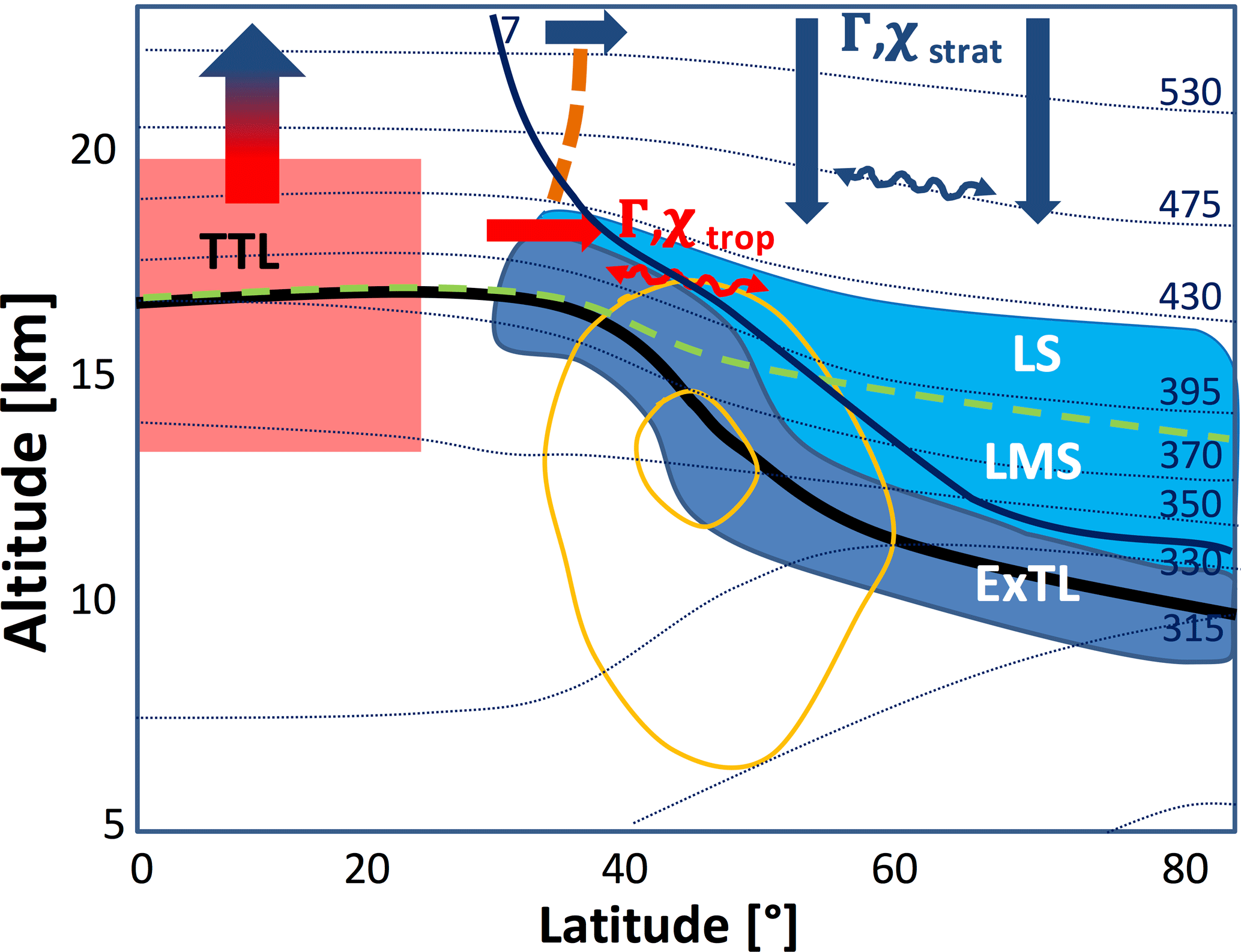
Figure 1Cross section of the Northern Hemispheric UTLS (upper troposphere – lower stratosphere) region, adapted from Riese et al. (2014) and Müller et al. (2016). The thermal tropopause is denoted by the thick black solid line. The measurement region is depicted as a blue box subdivided into the extratropical tropopause layer (ExTL), the lowermost stratosphere (LMS) and the lower stratosphere (LS). LMS and LS are separated by the 380 K isentrope (green dashed line). Transport pathways of air masses are denoted by coloured, thick arrows from the tropical tropopause layer (TTL) (red) and the polar Arctic upper stratosphere (blue) with respective mean age Γ and trace-gas volume mixing ratio χ. Quasi-horizontal mixing is represented by wavy double side arrows, indicating no net mass transport of air masses. Dotted lines are isentropes in K. The solid dark blue line indicates the 7 PVU contour, which is used to separate the regime of the ExTL from the LMS and LS (for details see text). Thin orange contour lines depict the zonal view of the jet stream.
Observations of SF6, N2O and CO2 from the ER-2 aircraft show that the mean age at northern high latitudes at an altitude of 20 km is of the order of 4–6 years (Andrews et al., 2001; Engel et al., 2002). Satellite observations of SF6 confirm this and show further a strong interannual variability in the mean age in northern high latitudes (Stiller et al., 2008, 2012; Haenel et al., 2015). The observations also indicate a potential transport of mesospheric air to lower altitudes (Engel et al., 2006b; Ray et al., 2017), which, however, strongly depends on the strength and persistence of the Arctic polar vortex during the individual winters.
In addition to diabatic descent inside and outside the polar vortex, quasi-isentropic mixing from lower latitudes leads to a contribution of relatively young air to the UTLS. As a result, a seasonal cycle of the chemical composition of the UTLS up to Θ=430 K establishes a relatively tropospheric character during northern summer/autumn and a more stratospheric characteristic in late winter/spring (Hegglin and Shepherd, 2007). The chemical composition and age structure of the extratropical UTLS (ExUTLS) are affected by the competing diabatic downwelling of aged air and rapid quasi-isentropic mixing down to the tropopause (Hoor et al., 2005; Engel et al., 2006a; Bönisch et al., 2009; Garny et al., 2014). The region between Θ=380 K and the bottom of the tropical pipe around Θ=450 K (Palazzi et al., 2011) is a key region for the transition between these transport regimes. The Θ=380 K isentrope coincides with the tropical tropopause and is therefore directly affected by diabatic vertical transport of tropospheric air through the tropical transition layer (TTL) (Fueglistaler et al., 2009) into the stratosphere. Above Θ=380 K these air masses, which ascended through the TTL are rapidly mixed quasi-horizontally by breaking planetary waves with air from high latitudes in addition to the shallow branch of the Brewer–Dobson circulation (Birner and Bönisch, 2011; Abalos et al., 2013). This rapid transport particularly modifies the abundance of water vapour and ozone in this region, which have seasonally varying isentropic gradients (Rosenlof et al., 1997; Randel et al., 2006; Hegglin and Shepherd, 2007; Pan et al., 2007; Ploeger et al., 2013).
In our study we focus on the transition of the tracer composition in the vortex-affected UTLS region up to Θ=410 K during winter 2015–2016. We will quantify the effects of quasi-isentropic mixing from the tropics and diabatic downwelling and its effect on the chemical composition as well as the evolution of the age spectrum and the mean age in this region.
The early Arctic winter of 2015–2016 (November–December) was among the coldest winters in the lower stratosphere (LS) after 1948. These extremely cold conditions existed due to a strong and cold Arctic polar vortex which developed in November 2015 due to very low planetary wave activity in the stratosphere (Matthias et al., 2016). From late December 2015 to early February 2016 the temperatures at Θ=490 K decreased to below 189 K. Therefore strong dehydration and denitrification were seen in low H2O and HNO3 volume mixing ratios, which finally led to a strong chlorine activation in early winter. Using MLS data the chemical influence of the vortex could be observed on isentropes below Θ=400 K (Manney and Lawrence, 2016).
The major final warming (MFW) (Manney and Lawrence, 2016) occurred on 5 March 2016, which led to the vortex splitting 1 week later. This early final warming was unusual, as only five other MFWs since 1958 have appeared before the middle of March. Due to this, early warming air masses in the polar lower stratosphere were mixed with non-vortex air and prevented chemical ozone depletion, reaching record low values during winter 2015–2016 (Manney and Lawrence, 2016, and references therein).
The winter of 2015–2016 was characterised by an unprecedented anomaly of the quasi-biannual oscillation (QBO) with a westerly jet that formed within the easterly phase in the lower stratosphere (Newman et al., 2016; Osprey et al., 2016). Since the QBO affects the zonal wind direction in the tropical lower stratosphere (Niwano et al., 2003) its strength and phase is crucial for stratospheric transport processes (Baldwin et al., 2001) and westerly phases are related to a strong and cold polar Arctic vortex (Holton and Tan, 1980).
Further the winter of 2015–2016 was also affected by a strong warm phase of the El Niño Southern Oscillation (ENSO) (Chen et al., 2016; L'Heureux et al., 2017). Matthias et al. (2016) argue that the strong El Niño weakened the 2016 Arctic vortex, while Palmeiro et al. (2017) found a connection of this ENSO event to the strong polar vortex and the easterly MFW.
This work will address the evolution of composition, age structure and the influence of transport and mixing of air masses in the lower stratosphere. The composition of air masses inside the LS, which is affected by diabatic descent of upper stratospheric air masses irreversibly mixed with younger air from the TTL, is analysed by combining measurements of in situ data with model calculations of the Chemical Lagrangian Model of the Stratosphere (CLaMS) (McKenna et al., 2002; Grooß et al., 2014; Ploeger et al., 2015).
3.1 The POLSTRACC campaign 2015–2016
The data presented in this study were obtained during the POLSTRACC (The Polar Stratosphere in a Changing Climate) mission, which was part of the combined PGS (POLSTRACC/GW-LCYCLE/SALSA) framework. The main objectives of the POLSTRACC mission were the investigation of structure, composition and dynamics of the Arctic LMS and processes involving chemical ozone depletion and polar stratospheric clouds in the Arctic winter UTLS. In total there were 17 scientific flights from December 2015 to the end of March 2016 on board the new German research aircraft HALO (High Altitude Long Range) from Oberpfaffenhofen, Germany (48.05∘ N, 11.16∘ E) and Kiruna, Sweden (67.49∘ N, 20.19∘ E), covering the region from 25 to 87∘ N and 24∘ E to 80∘ W (Fig. 2). Typical flight altitudes ranged from 10 to 14.5 km a.s.l.1, corresponding to potential temperatures in the stratosphere from Θ=320 K up to Θ=410 K. The total flight time was about 157 h, of which 19 h were in December 2015, 62 h were in January–February and 76 in February–March. For this study we focus on Arctic measurements starting from Kiruna, which took place during two campaign phases, representing flights from 12 January 2016 to 2 February 2016 (phase 1) and from 26 February 2016 to 18 March 2016 (phase 2). For this work we use approximately 50 h of measurements of those flights which were conducted to probe air masses above the extratropical transition region (ExTL) and underneath the polar vortex above PV = 7 PVU (1 PVU = 10−6 m2 s−1 K kg−1).
The research aircraft HALO is a modified business jet type Gulfstream G-550. It has a maximum range of 12 500 km with a maximum altitude of 15.5 km and can carry up to 3 t of scientific payload. The payload was a combination of different remote sensing (e.g. WALES lidar; Wirth et al., 2009; Fix et al., 2016; Väisälä RD 49 dropsondes and GLORIA limb sounder; Friedl-Vallon et al., 2014; Kaufmann et al., 2015) and in situ instruments that measured trace gases with different lifetimes, sources and sinks.
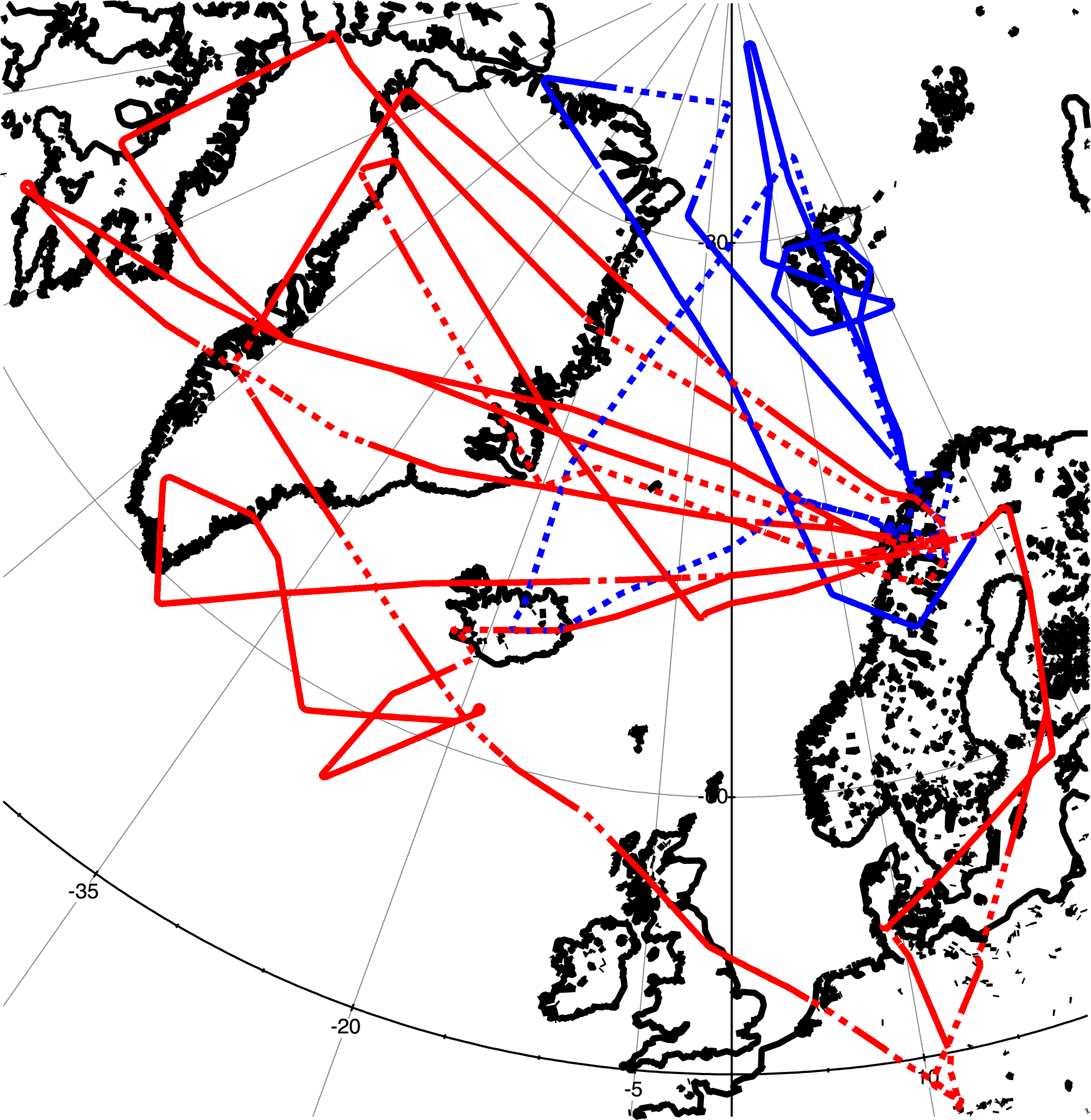
Figure 2Flight tracks during the POLSTRACC campaign. Blue colours indicate flights during phase 1 (12 January–2 February), red colours indicate flights during phase 2 (26 February–18 March). Flights that were used for the analysis are shown as solid lines. Dotted lines denote flight legs with PV < 7 PVU. For details see Sect. 3.1.
3.2 In situ trace-gas measurements
In this study we analyse measurements of N2O and CO, which were measured with the TRIHOP instrument (Müller et al., 2015) and SF6 by the GhOST-MS instrument (Sala et al., 2014). For our analysis the data are synchronised to a common time resolution of 0.1 Hz, corresponding to a horizontal resolution of 2.5 km at typical HALO flight speeds. GhOST data are available with a resolution of 60 s at an integration time of 1 s which leads to a horizontal resolution of 15 km.
3.2.1 The TRIHOP instrument
The TRIHOP instrument (Schiller et al., 2008) is an infrared absorption laser spectrometer with three quantum cascade lasers (QCL) operating between wave numbers 1269 and 2184 cm−1 and measures CO, N2O and CH4. The instrument uses a multipass white cell with a constant pressure of 30 hPa to minimise pressure broadening of the absorption lines. The three species are subsequently measured with an integration time of 1.5 s per species during a full cycle which finally leads to a time resolution of 7 s due to additional latency times when the channels are switched. In-flight calibration is performed against compressed ambient air standards that were calibrated against primary standards before and after the campaign. The primary standards are traceable to the World Meteorological Organisation Global Atmosphere Watch Central Calibration Laboratory (WMO GAW CCL) scale (X2007) for greenhouse gases. During POLSTRACC it was possible to achieve (2σ) precisions for CO, N2O and CH4 of 1.15, 1.84 and 9.46 ppbV.
3.2.2 GhOST-MS in situ measurements
The GHOST-MS instrument is a two-channel gas chromatograph for airborne measurements of trace gases. One channel uses a mass spectrometer (Agilent MSD 5975) for the detection of atmospheric trace gases at a time resolution of 4 min. This channel uses negative ion chemical ionisation as described in Sala et al. (2014) to measure brominated hydrocarbons. The other channel measures SF6 and CFC-12 using an ECD (electron capture detector) with a time resolution of 1 min. For the POLSTRACC campaign the precision for SF6 was 0.6 % and the precision for CFC-12 was 0.2 %.
The mean age of air is inferred from SF6 measurements (Engel et al., 2009). Due to its much higher atmospheric mixing ratio, the precision of CFC-12 measurements is better than that of SF6 measurements. Prior to calculating mean age, the SF6 time series has therefore been smoothed using the CFC-12, by applying a local (10 min of data before and after the time of measurement) fit between CFC-12 and SF6. This procedure removes parts of the instrumental scatter but retains the local information, particularly keeping the atmospheric variability (unlike averaging) and does not introduce any offset to the mean age values. Mean age derived in this way has an overall precision of better than 0.3 years and an estimated accuracy of 0.6 years, as explained in Engel et al. (2006a). Both SF6 and CFC-12 are reported on the SIO-2005 scale.
3.3 The Chemical Lagrangian Model of the Stratosphere (CLaMS)
The analysis of trace-gas measurements is complemented by simulations with the Chemical Lagrangian Model of the Stratosphere CLaMS (McKenna et al., 2002; Konopka et al., 2004). CLaMS is a Lagrangian chemistry transport model, based on forward-trajectory calculations and a parameterisation of small-scale atmospheric mixing which depends on the deformation rate of the large-scale flow. The model simulation is driven with meteorological data (e.g. horizontal wind fields) from European Centre of Medium Range Weather Forecasts (ECMWF) ERA-Interim reanalysis (Dee et al., 2011) and covers the period 1979–2017. The model uses an isentropic vertical coordinate throughout the stratosphere and the vertical velocity is deduced from the reanalysis total diabatic heating rate. Further details about the model set-up and the included chemical reactions (relevant species here are CO and N2O) are given in Pommrich et al. (2014). This long-term CLaMS simulation has been shown to reliably represent transport processes in the lower stratosphere for the relevant trace-gas species CO and N2O (Pommrich et al., 2014) as well as for mean age of air (Ploeger et al., 2015).
Recently, a method for calculating the age of air spectrum has been implemented in CLaMS (Ploeger and Birner, 2016), which will be used in the following analysis. The age spectrum is the transit time distribution of air masses for transport from a control surface (usually taken as the tropical tropopause or the Earth's surface) to a given location in the stratosphere (e.g. Hall and Plumb, 1994; Waugh, 2002) and can be related to the Green's function of the transport equation. The calculation method in CLaMS is based on inert tracer pulses, with different tracers released every other month at the surface in the tropics. This method allows the calculation of time-dependent age spectra for the non-stationary atmospheric flow at any location and time in the model domain (see Ploeger and Birner, 2016 for further details). Mean age in CLaMS is calculated from an inert model “clock tracer” with a linear increasing mixing ratio at the surface (Hall and Plumb, 1994). The resulting mean ages are fully consistent with mean age calculated as the first moment of the CLaMS age spectrum (Ploeger and Birner, 2016).
A CLaMS simulation with full stratospheric chemistry was integrated as described by Grooß et al. (2014). The upper boundary is set to Θ = 900 K potential temperature, where tracers like O3, N2O and CO are constrained by MLS satellite observations. Due to its Lagrangian formulation, a box-trajectory model set-up is also possible in which the identical chemistry scheme is used along single air mass trajectories. This set-up is also used here to diagnose chemical pathways and chemical conversion rates. This box model set-up is also used here to estimate CO production and loss rates.
As shown in Hoor et al. (2010) rapid and frequent mixing with tropospheric air mainly affects the region of PV < 7 PVU. To exclude mixing with air masses of recent tropospheric origin or from the exTL (extratropical tropopause layer) we only selected data above this level of potential vorticity. Therefore the composition of analysed data is mainly affected by isentropically, irreversibly mixed air mass signatures originating out of the tropics and diabatically descended air masses from the upper stratosphere in the polar region. In this analysis we further excluded flights which were dedicated to the observation of gravity waves.
4.1 Tracer distributions and mean age
Figures 3, 4 and 5 show tracer distributions as a function of equivalent latitude and potential temperature θ (Strahan et al., 1999; Hoor et al., 2004; Hegglin et al., 2006). Equivalent latitude is directly linked to the potential vorticity, which is conserved under adiabatic processes (Holton, 2004). Therefore, these coordinates are suitable for accounting for reversible adiabatic tracer transport.
4.1.1 Age of air
An air parcel in the stratosphere is a mixture of fractions of air with different histories, transport pathways and individual transit times. The transport pathways create an age spectrum or transit time distribution. The age spectrum can be obtained by calculation of the Green's function of the tracer continuity equation for a conserved and passive species (Hall and Plumb, 1994).
The mean age is defined as the first moment of the transit time distribution. To determine the mean age from long-lived tracer measurements, the tracer must have a well known source distribution at the tropical tropopause and a well defined vertical gradient in the stratosphere (Hall and Waugh, 1997). Since SF6 is a long-lived inert trace gas with a well known increase in its mean surface mixing ratio, it is commonly used for calculations of mean age (Bönisch et al., 2009). The sink of SF6 is in the mesosphere, where it is destroyed by shortwave UV radiation. The lifetime of SF6 is assumed to be 3200 years, but recent studies indicate a significantly shorter lifetime of about 850 years (Ray et al., 2017). This implies that the mean age derived from SF6 may be too old. Models and observations both show a high bias of up to 1 year in the polar vortex (Ray et al., 2017) or even more in mesospheric air (Engel et al., 2006b). Since we focus on the lower stratosphere far below the mesospheric loss region for SF6 and we further focus on age changes, our data are not affected by this fact.
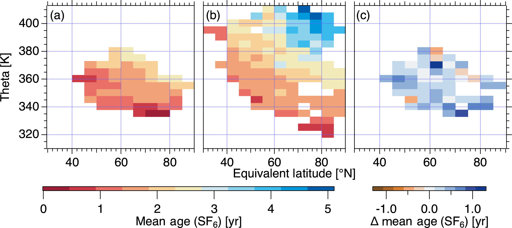
Figure 3Distributions of mean age from SF6 measurements in potential temperature – equivalent latitude coordinates for PV > 7 PVU. Panel (a) shows data for phase 1, (b) for phase 2 and panel (c) shows their absolute difference (phase 2 − phase 1). The colour code represents the mean age. Blue colours in panel (c) indicate an increase in mean age in the subvortex region from January to March. Only bins with more than 10 data points are shown.
Figure 3a and b show the distribution of mean age calculated from SF6 measurements for phase 1 (January) and phase 2 (February–March). Panel (a) shows that the LS during phase 1 is dominated by air masses of mean ages from 0.5 years to less than 3 years at maximum. The oldest air masses with mean ages above than 2 years were encountered furthest away from the tropopause and potential temperatures ranged from Θ=360 K to Θ=380 K. In contrast, during phase 2 (panel b) in general much older air masses, up to 5 years, were found at potential temperatures of Θ=410 K. These higher potential temperatures at flight altitude are the result of the diabatic descent over the course of the winter and indicate an increasing influence of air masses originating deeper in the stratosphere or from the Arctic polar vortex. To directly compare the temporal evolution of the age of air in the lower stratosphere, panel (c) shows the difference in age of air between both phases and shows that the bulk of the air inside the LS is ageing, to between Θ=330 K and Θ=380 K. The mean increase is 0.29 years, indicating diabatic downwelling due to the evolution of the polar vortex and thus an increased mean age in late winter.
4.1.2 Nitrous oxide
Nitrous oxide (N2O) has a lifetime of 123 years (Ko et al., 2013) and is released at the surface with no chemical sources in the atmosphere (Dils et al., 2006). As a result, N2O has a near-constant tropospheric value of 329.3 ppbV (winter 2015–2016 according to NOAA, 2017), which makes stratospheric influence identifiable (Müller et al., 2015). The mean annual tropospheric increase is currently approximately 0.78 ppbV per year (Hartmann et al., 2013).
The main sink reactions of N2O are due to photolysis in the UV band (190 nm 220 nm) and the reaction with O(1D), which only occurs within the upper stratosphere (Ko et al., 2013). Thus, N2O above the tropopause shows a weak negative vertical gradient which maximises during winter and spring due to the diabatic downwelling by the Brewer–Dobson circulation.
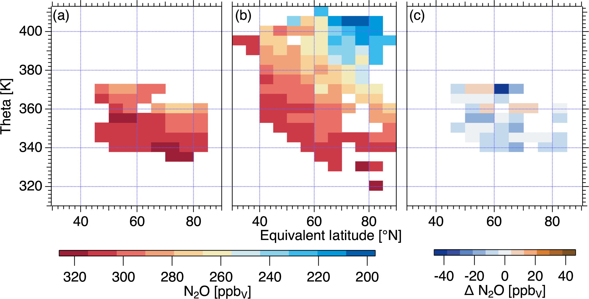
Figure 4a and b show N2O values between 276 and 325 ppbV measured during phase 1 and values below 200 ppbV measured during phase 2 above Θ = 400 K. Figure 4c shows an overall decrease in N2O in the polar lower stratosphere due to diabatic descent during winter, consistent with mean age changes (Fig. 3c).
4.1.3 Carbon monoxide
Carbon monoxide (CO) is released to the atmosphere mainly through incomplete combustion processes and methane oxidation as the only significant in situ source. Due to the high variability in anthropogenic surface emissions, CO mixing ratios in the Northern Hemisphere vary from 70 to 200 ppbV (Prinn et al., 2000) and the CO lifetime is of the order of weeks. In the lower stratosphere the main source of CO is methane oxidation with the OH radical. The main sink is oxidation by OH. The CO lifetime during polar night is a few months. In the stratosphere CO is controlled by production from methane oxidation and CO degradation. In the absence of transport from the troposphere this leads to an equilibrium between production and destruction of CO. We found an equilibrium value of 10–15 ppbV in winter 2015–2016, depending on the integrated temperature history of the respective air mass in agreement with previous studies (Müller et al., 2016; Herman et al., 1999).
The reaction of CH4 with Cl is an insignificant source of CO in the lower stratosphere (Flocke et al., 1999). Transport from the mesosphere, where CO is produced from the photolysis of CO2, also provides a potential source of CO via strong diabatic descent during winter under persistent polar vortices (Engel et al., 2006a). These potential influences are discussed in Sect. 6.
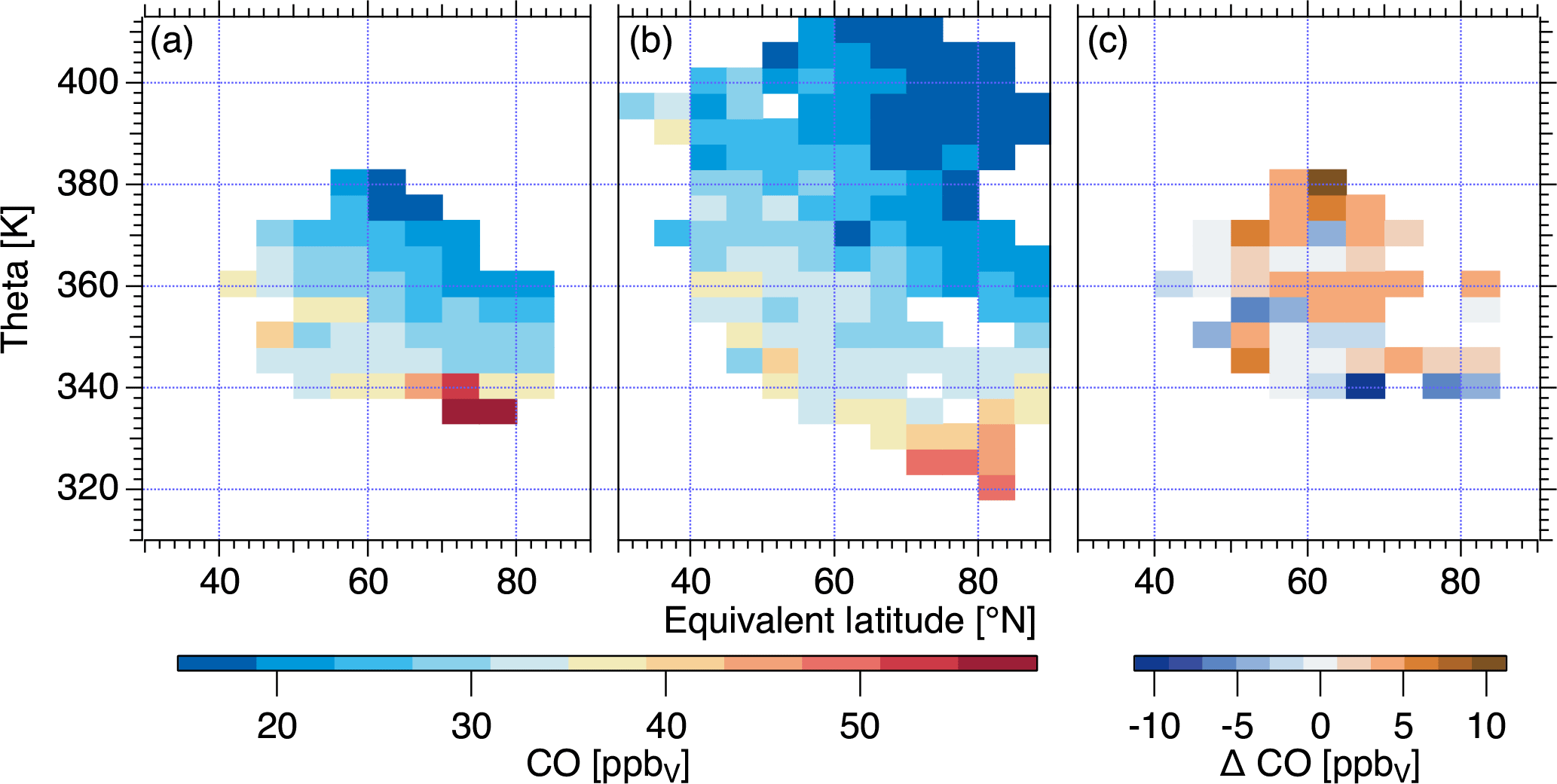
Figure 5 shows the distribution of CO. During phase 2 (panel b) the lowest mixing ratios of 15 ppbV were found at potential temperatures between Θ=380 K and Θ=410 K and equivalent latitudes > 60∘ N. As can be seen by the vertical branch of the CO–N2O correlation (Figs. 6 and 7), this value is the stratospheric equilibrium during late winter. Phase 1 (panel a) values ranged between 60 and 17 ppbV; hence the stratospheric background value was not measured in January 2016. A strong tropospheric influence is evident below Θ=340 K, with CO values up to 57 ppbV at phase 1 and 47 ppbV at phase 2. Hence the overall distribution of carbon monoxide in the UTLS during the individual phases (Fig. 4a and b) seems to be consistent with N2O and mean age obtained from SF6 measurements, despite its much shorter lifetime compared to the other species.
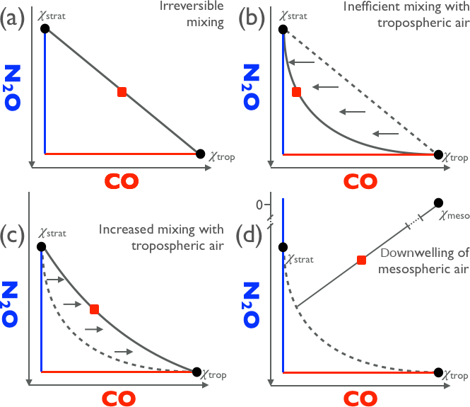
Figure 6Sketch of tracer–tracer correlations with different lifetimes. Note that the N2O axis is reversed. Panel (a) shows the L-shaped structure with an air parcel (red box) on a straight mixing line for fast mixing timescales. The horizontal red line represents the tropospheric N2O background, the blue vertical line the stratospheric CO equilibrium. Panel (b) shows the resulting curve in case of inefficient mixing compared to the chemical lifetime. Panel (c) shows the change in curvature depending on the strength of mixing and panel (d) shows the influence of the mesosphere on the correlation.
However, when comparing the differences in the respective phases (panel c), we see their behaviour is different to N2O and SF6. We encountered an increase in carbon monoxide mixing ratios over the course of the winter, which is at a first glance in contradiction to the distributions of mean age and N2O. While the distributions of long-lived tracers SF6 and N2O indicate an ageing of air masses, the increase in short-lived CO indicates a source of CO either from the troposphere or the stratosphere. Note that the increase is observed above Θ=360 K and 50∘ N equivalent latitude. Below Θ=360 K decreasing values are encountered. We will analyse the potential sources of CO in the following and suggest that CO increases due to an enhancement of mixing tropospheric air from the tropical lower stratosphere over the course of the winter without an increase in the upper tropospheric mixing ratios, which are affected by the surface emissions.
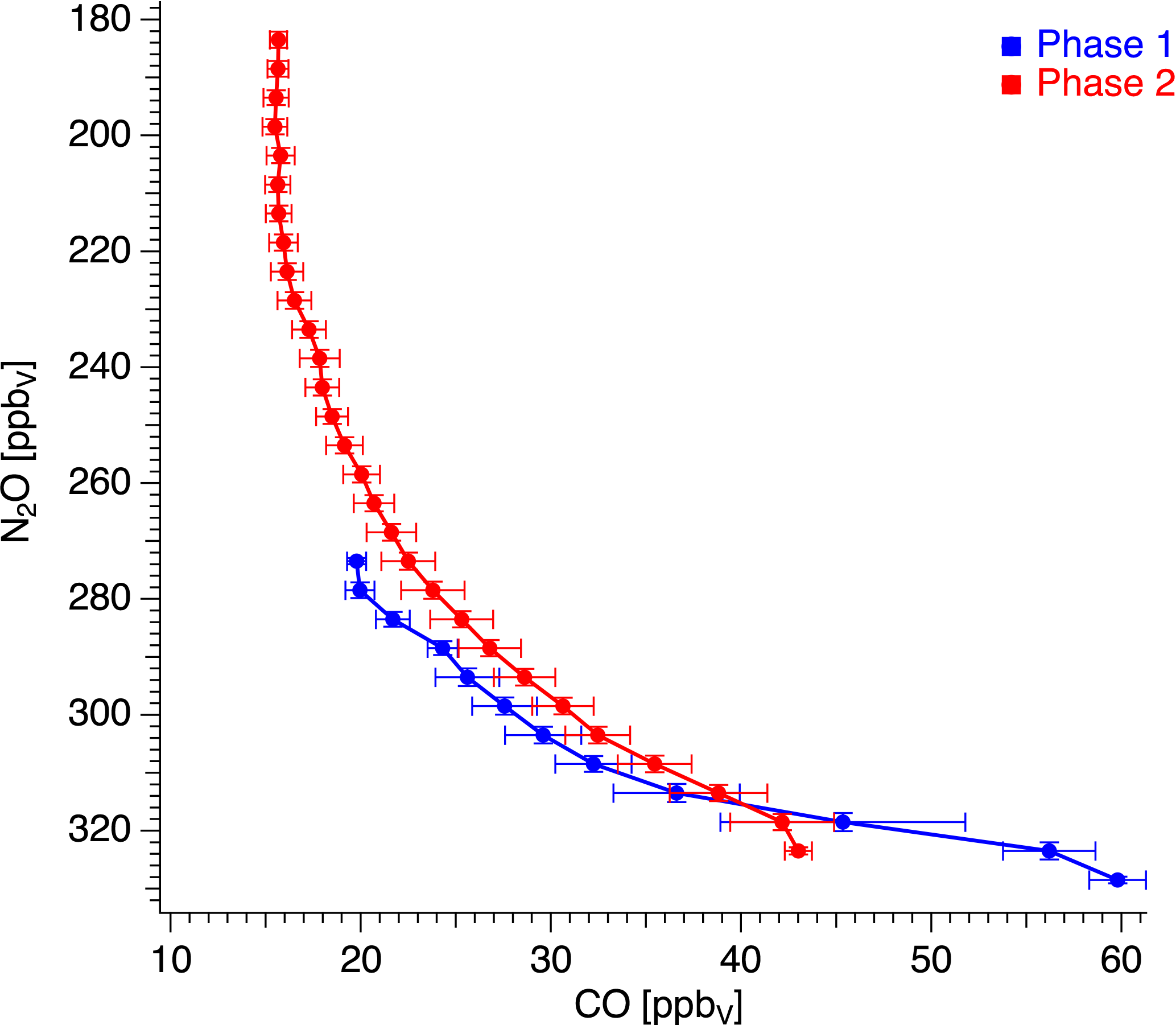
Figure 7N2O–CO correlation for POLSTRACC flights with PV > 7 PVU. The blue curve represents phase 1, the red curve represents phase 2. Data are binned in steps of 5 ppbV N2O. The variability in each bin is given by the vertical and horizontal lines.
We found a decrease in the long-lived species SF6 and N2O with their lowest values far above the local troposphere in late winter, which fits well in the general picture of enhanced downwelling of the Brewer–Dobson circulation in late winter–spring. The unexpected, simultaneous increase in the short-lived CO over the course of the winter could indicate a strengthening of tropospheric transport by enhanced mixing with air from the tropical lower stratosphere. In the following we will discuss this hypothesis and also other potential sources for the additional CO mixing ratios.
5.1 Identification of mixing on the basis of tracer–tracer correlations
To identify mixing processes across the tropopause CO-O3 correlations have been widely used (Fischer et al., 2000; Zahn et al., 2000; Hoor et al., 2002; Pan et al., 2004; Müller et al., 2016). Since ozone is affected by chemical processes, particularly in the vortex region, we use N2O as a stratospheric tracer instead of ozone. Carbon monoxide, used here as a tropospheric tracer, also has sources in the mesosphere and via chlorine chemistry in the stratosphere. In the LS the influence of chlorine is small compared to the reaction with the hydroxyl radical; therefore we investigated the influence of chlorine chemistry regarding methane which leads to the formation of CO. This influence will be discussed in detail later.
To analyse the effects of transport and mixing on the evolution of the UTLS composition we used the N2O–CO relation as shown in Fig. 6. Tropospheric data have high N2O values (> 328 ppbV) and are accompanied by high CO values, while stratospheric data have N2O < 328 ppbV. Due to the tropospheric background value of N2O and the stratospheric equilibrium of CO, the troposphere can be identified as the horizontal (high amount of N2O, variable CO) branch and the stratosphere, free of tropospheric influence can be identified as the vertical branch (low amount of CO, variable N2O) of the correlation. Without any recent mixing, the tracer–tracer correlation of N2O and CO would form an L-shaped structure (Fischer et al., 2000). In the presence of rapid mixing a straight mixing line between two end members of the correlation is established (panel a) (Hoor et al., 2002; Müller et al., 2016). As stratospheric CO will relax towards its stratospheric equilibrium value while N2O is long-lived in the lower stratosphere, the initial linear correlation will become curved with time in the case of inefficient mixing when the chemical lifetime is shorter than the timescale of mixing (panel b). Depending on the strength of mixing relative to the chemical CO sink the curvature will change and is less pronounced as the mixing becomes more efficient (panel c). It is important to note that the change in CO relative to a given N2O value can only be explained by a change in the ratio between mixing and chemical timescales. Mixing alone acts on both tracers N2O and CO. Therefore a change in the shape of the curve is a direct result of the increased mixing relative to the chemical timescale, which is less efficient when mixing becomes stronger. Figure 6d shows additionally the correlation under mesospheric-influenced conditions. In this case the correlation would rise to higher CO mixing ratios and lower N2O mixing ratios, since N2O gets destroyed and CO is produced in the mesosphere.
Figure 7 shows the N2O–CO correlation for POLSTRACC separated for phase 1 and phase 2, binned in intervals of 5 ppbV N2O. It is evident that tropospheric and stratospheric air masses are mixed in both phases. During phase 1 (blue curve) CO ranges between 20 ppbV and 60 ppbV at N2O values between 323 and 270 ppbV. Notably the red curve (phase 2) shows a steeper gradient with CO values between 43 and 15 ppbV at N2O values between 323 and 180 ppbV. There are higher CO mixing ratios for N2O values lower than 310 ppbV in phase 2 of the measurements. Additionally the red curve tends towards a CO equilibrium value of 15.67 ppbV for N2O values in the range of 220 to 180 ppbV.
Most importantly, there is an increase in CO on N2O isopleths between 313 and 273 ppbV N2O over the course of the winter. This is a remarkable result since we expect that due to the ageing of air inside the lower stratosphere in winter, the CO mixing ratio decreases with time. It is important to note that the correlation along the mixing line, which connects tropospheric values with the stratosphere, shows higher CO relative to N2O in phase 2. As indicated in Fig. 6 this is a clear indication of enhanced mixing of tropospheric air masses for N2O values > 273 ppbV. Furthermore phase 1 shows higher CO values relative to N2O compared to phase 2 for N2O values larger than 313 ppbV. Therefore we can conclude that regarding the CO–N2O correlation the tropospheric impact on short timescales through the ExTL was greater in phase 1 than in phase 2, indicating enhanced mixing with tropospheric-influenced air originating in the TTL region during phase 2.
A potential mesospheric impact is highly unlikely due to the fact that during phase 2 the N2O–CO correlation tends towards the equilibrium value in the region of lower N2O values. This influence will be discussed later in detail.
During both phases the UTLS between Θ=340 K and Θ=380 K was covered by our measurements. Therefore we assume the TTL (Fueglistaler et al., 2009) region (Fig. 1), where most of the tropospheric air masses are transported into the stratosphere (Schoeberl et al., 2006, and references therein) is the main source for the enhanced CO values (Fig. 5c). Further on, rapid eddy mixing of air from the TTL leads to an increase in tropospheric tracer signatures in the Arctic region (Rosenlof et al., 1997).
To quantify the increasing influence from tropospheric air masses in the lower stratosphere, we applied a simple mass balance approach to quantify the composition of the lower stratosphere. Therefore, we assume an air parcel in the lower stratosphere may consist of either upper stratospheric or tropospheric origin (Fig. 1). This mass balance system is solved to get the amount of tropospheric fraction ftrop of the measured air.
For a mixing ratio χ on a specific isentrope θ we assume
and
which leads to the tropospheric fraction ftrop based on CO measurements
with χCO,m the measured CO mixing ratio, χCO,strat the stratospheric CO background which was set to 15.7 ppbV as mean of the vertical branch of the CO–N2O correlation and χCO,trop the tropospheric CO entry value in the TTL.
In situ measurements have shown that CO mixing ratios above the tropical tropopause are at levels between 50 and 60 ppbV (Herman et al., 1999; Marcy et al., 2007).
Figure 8 shows the difference in the calculated tropospheric fraction ftrop between phase 2 and phase 1 as a function of N2O, which acts as a quasi-vertical coordinate. The CO increase over the course of the winter corresponds to an increase in ftrop of (6.8±3.7) % between 313 and 273 ppbV N2O by assuming 60 ppbV of CO at the tropical tropopause as provided by in situ aircraft data from Herman et al. (1999) and Marcy et al. (2007). Using COtrop = 80 ppbV as indicated by MLS at 100 hPa one obtains 32 % lower values for ftrop, which is still a significant increase in tropospheric air masses. Note that additionally the tropospheric fraction decreases towards more tropospheric N2O values from phase 1 to phase 2. This is clear evidence that an increase in the CO mixing ratio at the tropopause is not the cause of the observed lower stratospheric CO increase. This would be consistent with an increase in the fraction of young air of tropospheric origin and more efficient mixing as indicated in Fig. 6.
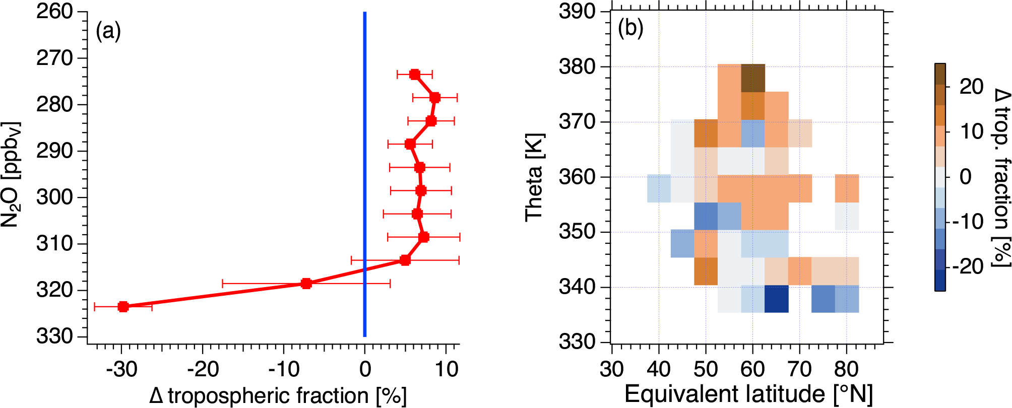
Figure 8(a) Tropospheric CO fraction from the mass balance equation as a function of N2O showing the difference between phase 2 and phase 1. (b) The same as panel (a) but as a distribution over equivalent latitude. Red colours indicate an increase in the tropospheric CO fraction.
Panel (b) shows the distribution against equivalent latitude. Note that the observed increase is most prominent above Θ=360 K. This is a clear indication that mixing at Θ<360 K is suppressed due to the strong subtropical jet, which acts as a barrier for mixing (Haynes and Shuckburgh, 2000) and would be consistent with enhanced mixing out of the TTL region.
5.2 Age spectra analysis
For further analysis of the relationship between diabatically descended, aged air with longer transit times and potentially mixed with young tropospheric air with shorter transit times we use age spectrum calculations of the CLaMS (Chemical Lagrangian Model of the Stratosphere) (McKenna et al., 2002; Ploeger et al., 2015; Ploeger and Birner, 2016) model, which gives information on the full transit time distribution. Notably we have the age spectral information for each individual data point along the flight track and therefore can directly compare our measurements with the spectrum.
To test whether the model is able to reproduce the observations of tracers we compared CO and N2O from CLaMS with the measurements (Fig. 9). Model output is available along the flight track with a time resolution of 10 s. Figure 9 shows the N2O–CO scatter plot for each data point. Panel (a) shows the correlation measured with the TRIHOP instrument, panel (b) shows the correlation calculated out of the CLaMS model. As is evident, CLaMS correctly represents the increase in CO relative to N2O from phase 1 to phase 2. Also, the separate branches of the two phases are reproduced and the crossing of the correlation at 40 ppbV CO and 310 ppbV N2O is consistently simulated.
This remarkable agreement between model and observations further motivates the usage of CLaMS for age analysis of our measurements.
As mentioned before, CLaMS is able to calculate the full transit time distribution of analysed air masses for each individual data point along the flight track. Figure 10 shows the averaged age spectra of the CLaMS model for the respective phase (panel a) and their difference (panel b). Vertical solid lines represent the mean age of the respective phase (blue and red) calculated by the CLaMS model, the dashed vertical lines separate young air masses with a mean age lower than 0.5 years from old air masses with mean age larger than 2 years. Since we have the full transit time distribution of each data point, we can compare this relation between the different parts of the age spectrum. An increase in the tropospheric fraction would be linked to an increase in the part of the age spectrum with low transit times as indicated by the observed increase in CO relative to N2O.
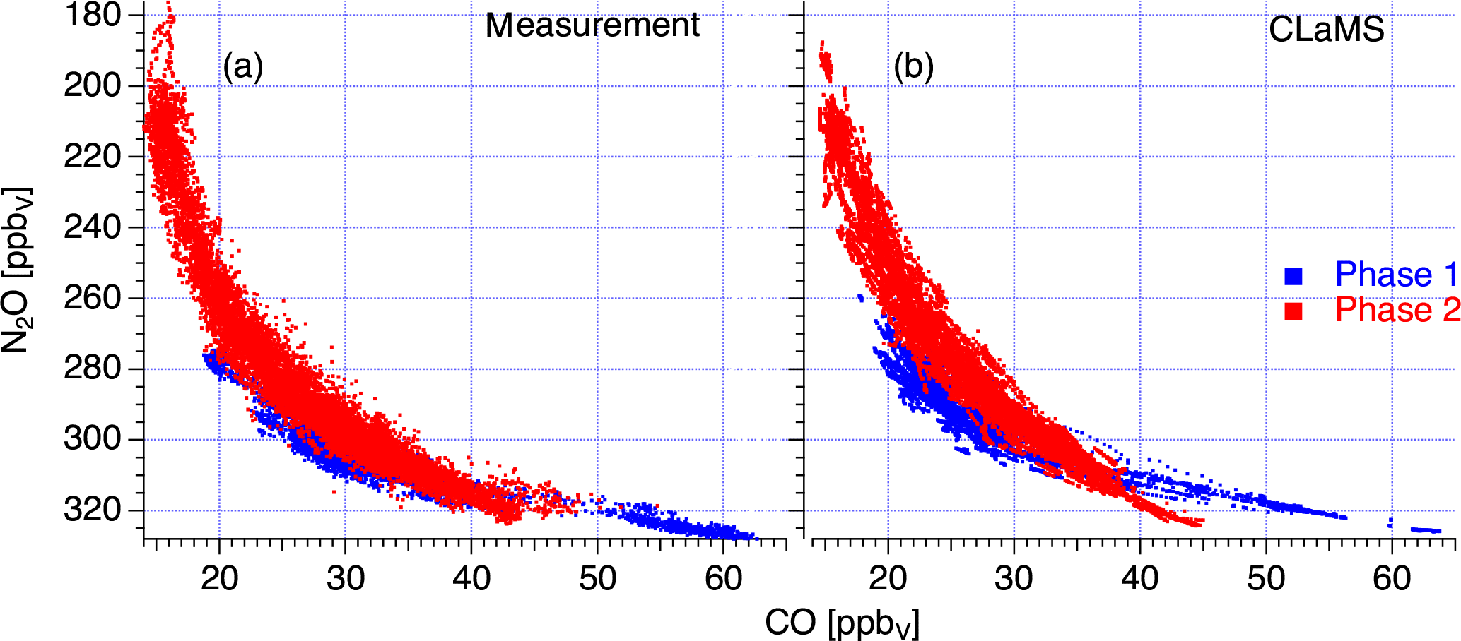
Figure 9N2O–CO scatter plot measured by the TRIHOP instrument (a) and CLaMS model output (b). Phase 1 coloured in blue, phase 2 coloured in red. The model output is available along the flight track with a time resolution of 10 s.

Figure 10(a) Averaged age spectra simulated by CLaMS for phase 1 (blue) and phase 2 (red). These spectra represent the mean of the individual age spectra available for each data point along the flight track. The mean age is indicated by the respective coloured vertical lines (phase 1: 1.71 years, phase 2: 1.98 years). The difference between the spectra is given in panel (b), showing an enhancement of young and old air masses from phase 1 to phase 2. Vertical dashed lines indicate the transit times of 6 months and 24 months (see next figures). The bin size of a data point is 1 month.
Figure 10 shows an absolute increase in air masses older than 2 years up to 0.3 % month−1. For air masses younger than 6 months, there is also an increase in the age spectrum between phase 2 and phase 1, with maximum values up to 0.9 % month−1, which is larger than the increase in the old air masses. The relative change in air masses younger than 6 months is 19.5 % and for air masses older than 2 years it is 76.4 %. The increase in the young fraction is in agreement with the observed CO increase, indicating increased mixing with air from the TTL at the end of winter.
Since the mean age is calculated as the first moment of the distribution, its value is most sensitive to changes in the old part (the so-called “old tail”) of the distribution (Hall and Waugh, 1997). Therefore the mean age rises by 0.27 years, from 1.71 to 1.98 years, as a result of the increase in the age spectrum distribution for air masses older than 2 years. This matches the mean age increase in SF6 and indicates, in agreement with the decrease in N2O, the overall ageing in the lower and lowermost stratosphere over the course of the winter. Since the integral over the Green's function is normalised to one, the increases of air masses older than 2 years and younger than 6 months must result in a relative decrease in between. Therefore air masses with mean ages between 0.5 and 2 years are more enhanced in phase 1 than in phase 2, which is evident by the change in the transit time distribution up to −1.9 % month−1.
To further investigate the relationship of young versus aged air, we calculated the accumulated fraction of air masses with transit times lower than 6 months and older than 2 years for each data point. Figure 11 shows the binned fraction of air masses with transit times under 6 months versus the modelled mean age.
The comparison of the scatter plot for different times (phase 1 and phase 2) shows that for a given mean age a significant increase in the young tropospheric contribution is evident. Thus, according to the model and in agreement with the observed increase in CO, the late winter LS is more affected by tropospheric young air. Therefore our results demonstrate that the mean age is an incomplete descriptor when referring to chemical properties of air masses involving different chemical lifetimes of species. Since the mean age is just a single number it might be insensitive to changes in the processes and timescales contributing to the mean, which, however, affect the chemical properties of the air parcel, e.g. by enhanced mixing of short-lived species. Therefore it is important to account for the full spectral shape when referring to chemical properties of an air mass rather than only the mean age.
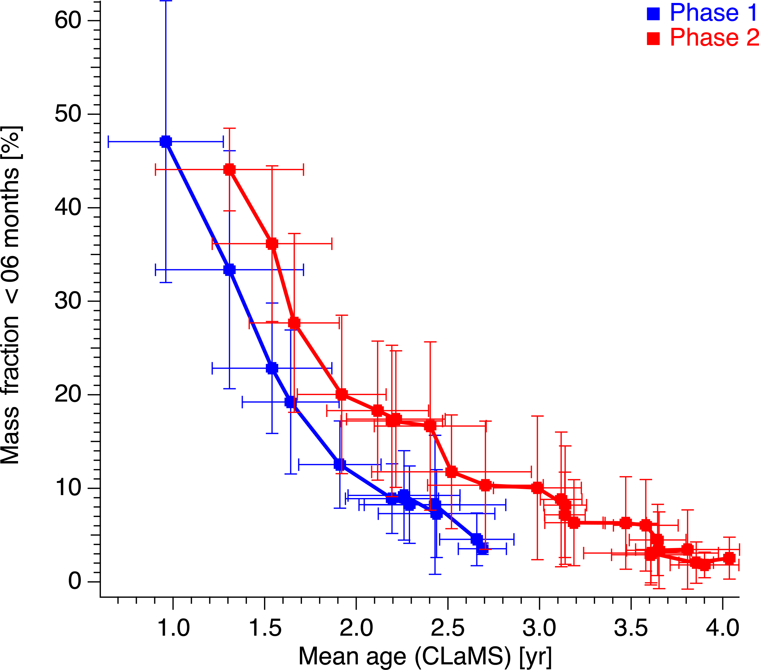
Figure 11Mean age versus air fractions with transit times < 6 months from the age spectra simulated by CLaMS for phase 1 (blue) and phase 2 (red). Each data point is binned in steps of 5 ppbV N2O. The variability in each bin is given by the vertical and horizontal lines.
During winter 2015–2016 CO mixing ratios in the LS increased from January to March while long-lived trace gases denote ageing of the LS. The analysis of CO–N2O correlations, the mass balance equation of irreversible mixing and transport pathways in the LS and model simulations points towards an increased influence of tropospheric air masses from the tropical lower stratosphere. Additional potential sources of CO in the LS are discussed in the following.
Since there are different sources for CO at different locations in the atmosphere, an increase in carbon monoxide mixing ratios can be due to (i) an increase in isentropic mixing out of the TTL, (ii) an increase in the tropospheric source strength, (iii) a potential influence of the mesosphere and (iv) a change in chemical reaction cycles due to higher amounts of reactive chlorine in the stratosphere. As already discussed the increase in enhanced tropospheric source emissions (ii) is highly unlikely (see Fig. 7). Since our analysis points to an increase in isentropic mixing out of the TTL (i), the possible influence of points (iii) and (iv) have to be further discussed.
Carbon monoxide is produced in the mesosphere due to the photo-dissociation of carbon dioxide. Therefore the composition of mesospheric air masses is clearly distinct from air mass composition of the stratosphere. Rinsland et al. (1999) found increased CO mixing ratios up to 90 ppbV at altitudes around 25 km or Θ=630–670 K and Engel et al. (2006b) found CO values of 600 ppbV at an altitude of 32 km. Both studies show very low N2O mixing ratios (< 50 ppbV). Although the authors found layers of mesospheric air descending down to 22 km, this is not evident for the Arctic winter of 2015–2016, and the lowest N2O mixing ratios are found to be of the order of 200 ppbV. This is reflected in the MLS observations that determine the CLaMS upper boundary at Θ=900 K potential temperature (Fig. 12). The simulation indicates the expected downward transport of mesospheric-influenced air, but down to Θ=600 K at the end of March 2016 in agreement with our observations. CO values minimise at the highest flight levels and equivalent latitudes.
Furthermore, an additional influence of descended mesospheric air into the lower stratosphere would lead to mixing lines very strongly differing from the observed relationship (see Fig. 6), which is not observed in agreement with the CLaMS N2O–CO scatter plot (Fig. 9).

Figure 12Temporal evolution of zonal mean CO for equivalent latitudes > 70∘ N simulated by CLaMS for winter 2015–2016.
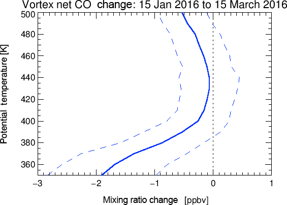
Figure 13Net change in CO from January to March for air masses in the Arctic vortex (equivalent latitude > 65∘ N) due to chemical reactions in the stratosphere and mesosphere calculated by CLaMS. The blue line represents the statistical mean, the dashed lines represent the 1σ standard deviation.
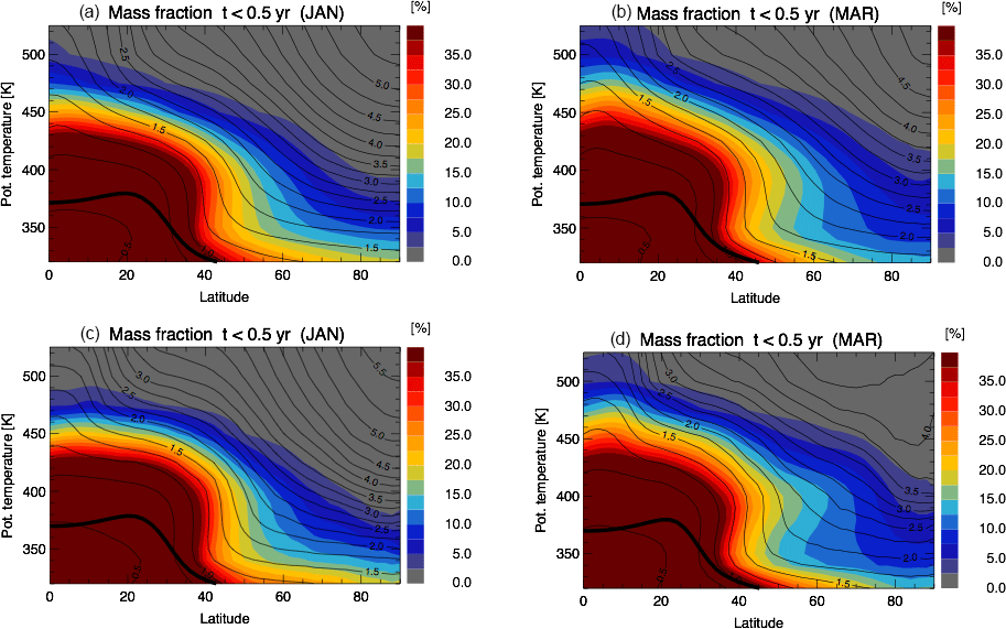
Figure 14Zonal mean of air mass fractions (colour code) with transit times < 0.5 years for January (a, c) and March (b, d) from 2004 to 2016 climatology (a, b) and for 2016 only (c, d) against potential temperature. The contour lines show mean age in years and the thick black line shows the WMO tropopause.
In general, another important source of carbon monoxide in the atmosphere is the reaction of methane with reactive chlorine, which is not significant in the lower stratosphere (Flocke et al., 1999). However, air masses enriched in reactive chlorine could have been transported downwards, providing potential reactants for the chemical production of CO. Therefore, we simulated the CO yield from the reactions of CH4 with chlorine, OH and O(1D) using CLaMS simulations in the box model mode. A large number of air parcel backward trajectories were calculated starting on 15 March from locations within the vortex core (equivalent latitude > 65∘ N; potential temperature between Θ=350 K and Θ=500 K). The trajectories ended on 15 January and the chemical composition changes were calculated using the CLaMS chemistry module running forward in time for a subset of the trajectories with equivalent latitudes greater 50∘ N on 15 January (21 480 trajectories). Figure 13 shows the statistical evaluation of the net CO change due to chemistry over the period as a function of potential temperature on 15 March. The blue line represents the statistical mean and the dashed lines represent the 1σ standard deviation. The mean overall change is even negative over the entire profile, which is due to the oxidation of the produced CO by the reaction with OH. Therefore we conclude that the observed increase in CO in phase 2 is not due to the additional chemical source reaction. The significant increase in air masses younger than 6 months (Fig. 11) also indicates a strong contribution of young rather than mesospheric air.
Figure 13 shows the statistical evaluation of the net CO change due to chemistry over the period as function of potential temperature on 15 March. The blue line represents the statistical mean and the dashed lines represent the 1σ standard deviation. As is evident the mean overall change is even negative over the entire profile, which is due to the oxidation of the produced CO by the reaction with OH. Therefore we conclude that the observed increase in CO in phase 2 is not due to the additional chemical source reaction.
To investigate whether transport and increased mixing of air mass fractions with transit times under 6 months in winter 2015–2016 was special compared to other years we analysed the climatology of these fractions from 2004 to 2016 and compared it to the calculated fractions in winter 2016. Both are from the CLaMS model (Fig. 14). The colour code represents the fractions of air masses with transit times under 6 months, the contour lines represent the mean age and the thick black line indicates the WMO tropopause.
The climatology shows that the largest fraction of air masses with transit times under 6 months exceeding 73 % is found between the equator and 30∘ N up to Θ=430 K. In January this strong signal has a sharp gradient at Θ=450 K. These air fractions are transported from January to March to the poles. As a result, northward of 70∘ N the fraction of air masses with transit times under 6 months increases by 5 % between Θ=360 K and Θ=420 K. From January 2016 to March 2016 this transport is even stronger than in the climatology, as shown by the different horizontal gradients in Fig. 14. The mean age in March compared to January at Θ=400 K shows a higher value in both the climatology and the winter of 2015–2016, whereas the structure of the mean age contours show a more horizontal meridional gradient in the winter 2016 compared to the climatology.
Finally, these findings highlight the role of mixing of young air in the lower stratosphere of the polar Arctic region with an underlying increase in mean age of air, indicating downward transported air masses of older air fractions. The enhanced transport of young air is evident from the climatology and turns out to be particularly strong in winter 2016.
We present tracer measurements of CO and N2O measured during the POLSTRACC campaign in winter 2015–2016 on board the German HALO research aircraft. The winter of 2015–2016 was characterised by an extremely cold and stable polar vortex which broke up due to an MFW on 5 March 2016. In combination with measurements of SF6 and model simulations by the CLaMS model it was possible to analyse the contributions of diabatic transport and isentropic mixing in the UTLS region. The mixing ratios of the long-lived trace gases N2O and SF6 decreased over the course of the winter and therefore denoted an overall ageing due to subsiding air masses in the Arctic polar lower stratosphere. The calculated mean age based on measured SF6 shows an ageing of 0.29 years (see Fig. 3c) and for CLaMS of 0.27 years (see Fig. 10a). Remarkably, the short-lived species CO increases at the same time. Since mixing can be identified by tracer–tracer correlations we used CO–N2O correlations to quantify the relation between transport and chemistry. Our analysis shows an increase of 3.7 ppbV CO relative to N2O, which can be linked to an increase of 6.8 % of mixed air masses out of the TTL region. The comparison with the CLaMS model shows a very good agreement between measurements and model calculations. The CO–N2O correlation is well reproduced by the model. Analysis of the averaged age spectrum for the respective phase shows that there is a simultaneous increase in fractions of air with transit times longer than 2 years and fractions of air with transit times smaller than 6 months. Since the mean age itself is most sensitive to changes on the old tail of the age spectrum, the ageing of air masses in the LS over the course of the winter can be explained by the increase in old air masses, characterised by low N2O and SF6 measurements. Increased mixing of young air masses adds to this and leads to an increased fraction of the younger part of the age spectrum, which is consistent with the observed increase in CO. It is evident that this enhancement is due to stronger mixing processes out of the TTL region, where fresh tropospheric air is mixed into the polar lower stratosphere. Other potential sources of CO like mesospheric air and the chemical reaction of CH4 with chlorine are unlikely to have caused the observed increase in CO.
Therefore we conclude that the Arctic lower stratosphere in March was strongly affected by mixing with young tropospheric air, which partly compensates for the overall ageing. These aged air masses are isentropically mixed with younger air masses out of the TTL region. The observations are in line with the climatology of mixing from 2004 to 2015 on the basis of ERA-Interim by the CLaMS model and highlight the importance of horizontal mixing from the tropics for the Arctic winter UTLS.
The observational data used in this study can be downloaded from the HALO database (https://doi.org/10.17616/R39Q0T; HALO consortium, 2018) at https://halo-db.pa.op.dlr.de/.
JK carried out the measurements and analysed the data with the help of PH. FP and JUG did the model simulations with the CLaMS model. AE, HB and TK provided the measurement data of SF6 and mean age. PH, AE, FP and JUG provided helpful discussions and comments. JK and PH wrote the manuscript. HO, BMS and WW coordinated the POLSTRACC project.
The authors declare that they have no conflict of interest.
This article is part of the special issue “The Polar Stratosphere in a Changing Climate (POLSTRACC) (ACP/AMT inter-journal SI)”. It is not associated with a conference.
This work was supported by the Deutsche Forschungsgemeinschaft (DFG, FKZ EN 367/13-1 and EN 367/11) and the Johannes Gutenberg-University Mainz (FKZ 8585084).
Jens Krause was partly funded under DFG grant HO 4225/7-1.
AGAGE is supported principally by NASA (USA) grants to MIT and SIO, and also
by DECC (UK) and NOAA (USA) grants to Bristol University, CSIRO and BoM
(Australia), FOEN grants to Empa (Switzerland), NILU (Norway), SNU (Korea),
CMA (China), NIES (Japan) and Urbino University (Italy).
Edited by: Martyn Chipperfield
Reviewed by: Eric Ray and two anonymous referees
Abalos, M., Randel, W. J., Kinnison, D. E., and Serrano, E.: Quantifying tracer transport in the tropical lower stratosphere using WACCM, Atmos. Chem. Phys., 13, 10591–10607, https://doi.org/10.5194/acp-13-10591-2013, 2013. a
Andrews, A. E., Boering, K. A., Daube, B. C., Wofsy, S. C., Hintsa, E. J., Weinstock, E. M., and Bui, T. P.: Empirical age spectra for the lower tropical stratosphere from in situ observations of CO2: Implications for stratospheric transport, J. Geophys. Res.-Atmos., 104, 26581–26595, https://doi.org/10.1029/1999JD900150, 1999. a
Andrews, A. E., Boering, K. A., Daube, B. C., Wofsy, S. C., Loewenstein, M., Jost, H., Podolske, J. R., Webster, C. R., Herman, R. L., Scott, D. C., Flesch, G. J., Moyer, E. J., Elkins, J. W., Dutton, G. S., Hurst, D. F., Moore, F. L., Ray, E. A., Romashkin, P. A., and Strahan, S. E.: Mean ages of stratospheric air derived from in situ observations of CO2, CH4, and N2O, J. Geophys. Res.-Atmos., 106, 32295–32314, https://doi.org/10.1029/2001JD000465, 2001. a
Baldwin, M. P., Gray, L. J., Dunkerton, T. J., Hamilton, K., Haynes, P. H., Randel, W. J., Holton, J. R., Alexander, M. J., Hirota, I., Horinouchi, T., Jones, D. B. A., Kinnersley, J. S., Marquardt, C., Sato, K., and Takahashi, M.: The quasi-biennial oscillation, Rev. Geophys., 39, 179–229, https://doi.org/10.1029/1999RG000073, 2001. a
Birner, T. and Bönisch, H.: Residual circulation trajectories and transit times into the extratropical lowermost stratosphere, Atmos. Chem. Phys., 11, 817–827, https://doi.org/10.5194/acp-11-817-2011, 2011. a, b
Bönisch, H., Engel, A., Curtius, J., Birner, Th., and Hoor, P.: Quantifying transport into the lowermost stratosphere using simultaneous in-situ measurements of SF6 and CO2, Atmos. Chem. Phys., 9, 5905–5919, https://doi.org/10.5194/acp-9-5905-2009, 2009. a, b, c
Brewer, A. W.: Evidence for a world circulation provided by the measurements of helium and water vapor distribution in the stratosphere, Q. J. Roy. Meteor. Soc., 75, 351–363, 1949. a
Butchart, N.: The Brewer-Dobson circulation, Rev. Geophys., 52, 157–184, https://doi.org/10.1002/2013RG000448, 2014. a
Chen, S., Wu, R., Chen, W., Yu, B., and Cao, X.: Genesis of westerly wind bursts over the equatorial western Pacific during the onset of the strong 2015–2016 El Niño, Atmos. Sci. Lett., 17, 384–391, https://doi.org/10.1002/asl.669, 2016. a
Dee, D. P., Uppala, S. M., Simmons, A. J., Berrisford, P., Poli, P., Kobayashi, S., Andrae, U., Balmaseda, M. A., Balsamo, G., Bauer, P., Bechtold, P., Beljaars, A. C. M., van de Berg, L., Bidlot, J., Bormann, N., Delsol, C., Dragani, R., Fuentes, M., Geer, A. J., Haimberger, L., Healy, S. B., Hersbach, H., Hólm, E. V., Isaksen, L., Kållberg, P., Köhler, M., Matricardi, M., McNally, A. P., Monge-Sanz, B. M., Morcrette, J.-J., Park, B.-K., Peubey, C., de Rosnay, P., Tavolato, C., Thépaut, J.-N., and Vitart, F.: The ERA-Interim reanalysis: configuration and performance of the data assimilation system, Q. J. Roy. Meteor. Soc., 137, 553–597, https://doi.org/10.1002/qj.828, 2011. a
Dils, B., De Mazière, M., Müller, J. F., Blumenstock, T., Buchwitz, M., de Beek, R., Demoulin, P., Duchatelet, P., Fast, H., Frankenberg, C., Gloudemans, A., Griffith, D., Jones, N., Kerzenmacher, T., Kramer, I., Mahieu, E., Mellqvist, J., Mittermeier, R. L., Notholt, J., Rinsland, C. P., Schrijver, H., Smale, D., Strandberg, A., Straume, A. G., Stremme, W., Strong, K., Sussmann, R., Taylor, J., van den Broek, M., Velazco, V., Wagner, T., Warneke, T., Wiacek, A., and Wood, S.: Comparisons between SCIAMACHY and ground-based FTIR data for total columns of CO, CH4, CO2 and N2O, Atmos. Chem. Phys., 6, 1953–1976, https://doi.org/10.5194/acp-6-1953-2006, 2006. a
Dobson, G. M. B.: Origin and Distribution of the Polyatomic Molecules in the Atmosphere, P. Roy. Soc. Lond. A Mat., Physical and Engineering Sciences, 236, 187–193, https://doi.org/10.1098/rspa.1956.0127, 1956. a
Ehhalt, D. H., Rohrer, F., Blake, D. R., Kinnison, D. E., and Konopka, P.: On the use of nonmethane hydrocarbons for the determination of age spectra in the lower stratosphere, J. Geophys. Res.-Atmos., 112, 1–12, https://doi.org/10.1029/2006JD007686, 2007. a
Engel, A., Strunk, M., Müller, M., Haase, H.-P., Poss, C., Levin, I., and Schmidt, U.: Temporal development of total chlorine in the high-latitude stratosphere based on reference distributions of mean age derived from CO2 and SF6, J. Geophys. Res.-Atmos., 107, ACH 1-1–ACH 1-11, https://doi.org/10.1029/2001JD000584, 2002. a, b
Engel, A., Bönisch, H., Brunner, D., Fischer, H., Franke, H., Günther, G., Gurk, C., Hegglin, M., Hoor, P., Königstedt, R., Krebsbach, M., Maser, R., Parchatka, U., Peter, T., Schell, D., Schiller, C., Schmidt, U., Spelten, N., Szabo, T., Weers, U., Wernli, H., Wetter, T., and Wirth, V.: Highly resolved observations of trace gases in the lowermost stratosphere and upper troposphere from the Spurt project: an overview, Atmos. Chem. Phys., 6, 283–301, https://doi.org/10.5194/acp-6-283-2006, 2006a. a, b, c
Engel, A., Möbius, T., Haase, H.-P., Bönisch, H., Wetter, T., Schmidt, U., Levin, I., Reddmann, T., Oelhaf, H., Wetzel, G., Grunow, K., Huret, N., and Pirre, M.: Observation of mesospheric air inside the arctic stratospheric polar vortex in early 2003, Atmos. Chem. Phys., 6, 267–282, https://doi.org/10.5194/acp-6-267-2006, 2006b. a, b, c
Engel, A., Möbius, T., Bönisch, H., Schmidt, U., Heinz, R., Levin, I., Atlas, E., Aoki, S., Nakazawa, T., Sugawara, S., Moore, F., Hurst, D., Elkins, J., Schauffler, S., Andrews, A., and Boering, K.: Age of stratospheric air unchanged within uncertainties over the past 30 years, Nat. Geosci., 2, 28–31, https://doi.org/10.1038/ngeo388, 2009. a
Fischer, H., Wienhold, F. G., Hoor, P., Bujok, O., Schiller, C., Siegmund, P., Ambaum, M., Scheeren, H. A., and Lelieveld, J.: Tracer correlations in the northern high latitude lowermost stratosphere: Influence of cross-tropopause mass exchange, Geophys. Res. Lett., 27, 97–100, https://doi.org/10.1029/1999GL010879, 2000. a, b
Fix, A., Amediek, A., Ehret, G., Groß, S., Kiemle, C., Reitebuch, O., and Wirth, M.: On the benefit of airborne demonstrators for space borne lidar missions, in: International Conference on Space Optics – ICSO 2016, 18–21 October 2016, Biarritz, France, Proceedings, 10562, 105621W, https://doi.org/10.1117/12.2296197, 2016. a
Flocke, F., Herman, R., and Salawitch, R.: An examination of chemistry and transport processes in the tropical lower stratosphere using observations of long-lived and short-lived compounds obtained during STRAT and POLARIS, J. Geophys. Res., 104, 26625–26642, https://doi.org/10.1029/1999JD900504, 1999. a, b
Friedl-Vallon, F., Gulde, T., Hase, F., Kleinert, A., Kulessa, T., Maucher, G., Neubert, T., Olschewski, F., Piesch, C., Preusse, P., Rongen, H., Sartorius, C., Schneider, H., Schönfeld, A., Tan, V., Bayer, N., Blank, J., Dapp, R., Ebersoldt, A., Fischer, H., Graf, F., Guggenmoser, T., Höpfner, M., Kaufmann, M., Kretschmer, E., Latzko, T., Nordmeyer, H., Oelhaf, H., Orphal, J., Riese, M., Schardt, G., Schillings, J., Sha, M. K., Suminska-Ebersoldt, O., and Ungermann, J.: Instrument concept of the imaging Fourier transform spectrometer GLORIA, Atmos. Meas. Tech., 7, 3565–3577, https://doi.org/10.5194/amt-7-3565-2014, 2014. a
Fueglistaler, S., Dessler, A. E., Dunkerton, T. J., Folkins, I., Fu, Q., and Mote, P. W.: Tropical tropopause layer, Rev. Geophys., 47, RG1004, https://doi.org/10.1029/2008RG000267, 2009. a, b
Garny, H., Birner, T., Bönisch, H., and Bunzel, F.: The effects of mixing on age of air, J. Geophys. Res.-Atmos., 119, 7015–7034, https://doi.org/10.1002/2013JD021417, 2014. a
Grooß, J.-U., Engel, I., Borrmann, S., Frey, W., Günther, G., Hoyle, C. R., Kivi, R., Luo, B. P., Molleker, S., Peter, T., Pitts, M. C., Schlager, H., Stiller, G., Vömel, H., Walker, K. A., and Müller, R.: Nitric acid trihydrate nucleation and denitrification in the Arctic stratosphere, Atmos. Chem. Phys., 14, 1055–1073, https://doi.org/10.5194/acp-14-1055-2014, 2014. a, b
Haenel, F. J., Stiller, G. P., von Clarmann, T., Funke, B., Eckert, E., Glatthor, N., Grabowski, U., Kellmann, S., Kiefer, M., Linden, A., and Reddmann, T.: Reassessment of MIPAS age of air trends and variability, Atmos. Chem. Phys., 15, 13161–13176, https://doi.org/10.5194/acp-15-13161-2015, 2015. a
Hall, T. M. and Plumb, R. A.: Age as a diagnostic of stratospheric transport, J. Geophys. Res.-Atmos., 99, 1059–1070, https://doi.org/10.1029/93JD03192, 1994. a, b, c, d, e
Hall, T. M. and Waugh, D. W.: Timescales for the stratospheric circulation derived from tracers, J. Geophys. Res., 102, 8991–9001, https://doi.org/10.1029/96JD03713, 1997. a, b
HALO consortium: High Altitude and LOng Range database, https://doi.org/10.17616/R39Q0T, last access: 27 April 2018. a
Hartmann, D. J., Klein Tank, A. M. G., Rusticucci, M., Alexander, L. V., Brönnimann, S., Charabi, Y. A.-R., Dentener, F. J., Dlugokencky, E. J., Easterling, D. R., Kaplan, A., Soden, B. J., Thorne, P. W., Wild, M., and Zhai, P.: Observations: Atmosphere and Surface, Clim. Chang. 2013 Phys. Sci. Basis. Contrib. Work. Gr. I to Fifth Assess. Rep. Intergov. Panel Clim. Chang., 159–254, https://doi.org/10.1017/CBO9781107415324.008, 2013. a
Haynes, P. and Shuckburgh, E.: Effective diffusivity as a diagnostic of atmospheric transport: 1. Stratosphere, J. Geophys. Res., 105, 22777, https://doi.org/10.1029/2000JD900093, 2000. a
Haynes, P. H., McIntyre, M. E., Shepherd, T. G., Marks, C. J., and Shine, K. P.: On the “Downward Control” of Extratropical Diabatic Circulations by Eddy-Induced Mean Zonal Forces, J. Atmos. Sci., 48, 651–678, https://doi.org/10.1175/1520-0469(1991)048<0651:OTCOED>2.0.CO;2, 1991. a
Hegglin, M. and Shepherd, T.: O3-N2O correlations from the Atmospheric Chemistry Experiment: Revisiting a diagnostic of transport and chemistry in the stratosphere, J. Geophys. Res., 112, 1–15, https://doi.org/10.1029/2006JD008281, 2007. a, b
Hegglin, M. I., Brunner, D., Peter, T., Hoor, P., Fischer, H., Staehelin, J., Krebsbach, M., Schiller, C., Parchatka, U., and Weers, U.: Measurements of NO, NOy, N2O, and O3 during SPURT: implications for transport and chemistry in the lowermost stratosphere, Atmos. Chem. Phys., 6, 1331–1350, https://doi.org/10.5194/acp-6-1331-2006, 2006. a
Herman, R., Webster, C., May, R., Scott, D., Hu, H., Moyer, E., Wennberg, P., Hanisco, T., Lanzendorf, E., Salawitch, R., Yung, Y., Margitan, J., and Bui, T.: Measurements of CO in the upper troposphere and lower stratosphere, Chemosphere – Global Change Science, 1, 173–183, https://doi.org/10.1016/S1465-9972(99)00008-2, 1999. a, b, c
Holton, J. R.: An introduction to dynamic meteorology, Elsevier Academic Press, Seattle, Washington, USA, 2004. a
Holton, J. R. and Tan, H.-C.: The Influence of the Equatorial Quasi-Biennial Oscillation on the Global Circulation at 50 mb, J. Atmos. Sci., 37, 2200–2208, https://doi.org/10.1175/1520-0469(1980)037<2200:TIOTEQ>2.0.CO;2, 1980. a
Holton, J. R., Haynes, P., and Mcintyre, M.: Stratosphere-Troposphere Exchange, Rev. Geophys., 33, 403–439, 1995. a
Hoor, P., Fischer, H., Lange, L., Lelieveld, J., and Brunner, D.: Seasonal variations of a mixing layer in the lowermost stratosphere as identified by the CO-O3 correlation from in situ measurements, J. Geophys. Res.-Atmos., 107, 1-1–1-11, https://doi.org/10.1029/2000JD000289, 2002. a, b
Hoor, P., Gurk, C., Brunner, D., Hegglin, M. I., Wernli, H., and Fischer, H.: Seasonality and extent of extratropical TST derived from in-situ CO measurements during SPURT, Atmos. Chem. Phys., 4, 1427–1442, https://doi.org/10.5194/acp-4-1427-2004, 2004. a
Hoor, P., Fischer, H., and Lelieveld, J.: Tropical and extratropical tropospheric air in the lowermost stratosphere over Europe: A CO-based budget, Geophys. Res. Lett., 32, L07802, https://doi.org/10.1029/2004GL022018, 2005. a
Hoor, P., Wernli, H., Hegglin, M. I., and Bönisch, H.: Transport timescales and tracer properties in the extratropical UTLS, Atmos. Chem. Phys., 10, 7929–7944, https://doi.org/10.5194/acp-10-7929-2010, 2010. a
Hoskins, B. J.: Towards a PV-theta view of the general circulation, Tellus A, 43, 27–35, https://doi.org/10.1034/j.1600-0870.1991.t01-3-00005.x, 1991. a
Kaufmann, M., Blank, J., Guggenmoser, T., Ungermann, J., Engel, A., Ern, M., Friedl-Vallon, F., Gerber, D., Grooß, J. U., Guenther, G., Höpfner, M., Kleinert, A., Kretschmer, E., Latzko, Th., Maucher, G., Neubert, T., Nordmeyer, H., Oelhaf, H., Olschewski, F., Orphal, J., Preusse, P., Schlager, H., Schneider, H., Schuettemeyer, D., Stroh, F., Suminska-Ebersoldt, O., Vogel, B., M. Volk, C., Woiwode, W., and Riese, M.: Retrieval of three-dimensional small-scale structures in upper-tropospheric/lower-stratospheric composition as measured by GLORIA, Atmos. Meas. Tech., 8, 81–95, https://doi.org/10.5194/amt-8-81-2015, 2015. a
Ko, M. K. W., Newman, P. A., Reimann, S., and Strahan, S. E.: SPARC Report, No. 6, 256 pp., available at: http://www.sparc-climate.org/publications/sparc-reports/ (last access: 4 April 2018), 2013. a, b
Konopka, P., Steinhorst, H.-M., Grooß, J.-U., Günther, G., Müller, R., Elkins, J. W., Jost, H.-J., Richard, E., Schmidt, U., Toon, G., and McKenna, D. S.: Mixing and ozone loss in the 1999–2000 Arctic vortex: Simulations with the three-dimensional Chemical Lagrangian Model of the Stratosphere (CLaMS), J. Geophys. Res.-Atmos., 109, D02315, https://doi.org/10.1029/2003JD003792, 2004. a
L'Heureux, M. L., Takahashi, K., Watkins, A. B., Barnston, A. G., Becker, E. J., Di Liberto, T. E., Gamble, F., Gottschalck, J., Halpert, M. S., Huang, B., Mosquera-Vásquez, K., and Wittenberg, A. T.: Observing and Predicting the 2015/16 El Niño, B. Am. Meteorol. Soc., 98, 1363–1382, https://doi.org/10.1175/BAMS-D-16-0009.1, 2017. a
Manney, G. L. and Lawrence, Z. D.: The major stratospheric final warming in 2016: dispersal of vortex air and termination of Arctic chemical ozone loss, Atmos. Chem. Phys., 16, 15371–15396, https://doi.org/10.5194/acp-16-15371-2016, 2016. a, b, c
Marcy, T., Popp, P., Gao, R., Fahey, D., Ray, E., Richard, E., Thompson, T., Atlas, E., Loewenstein, M., Wofsy, S., Park, S., Weinstock, E., Swartz, W., and Mahoney, M.: Measurements of trace gases in the tropical tropopause layer, Atmos. Environ., 41, 7253–7261, https://doi.org/10.1016/j.atmosenv.2007.05.032, 2007. a, b
Matthias, V., Dörnbrack, A., and Stober, G.: The extraordinarily strong and cold polar vortex in the early northern winter 2015/2016, Geophys. Res. Lett., 43, 12287–12294, https://doi.org/10.1002/2016GL071676, 2016. a, b
McKenna, D. S., Konopka, P., Grooß, J.-U., Günther, G., Müller, R., Spang, R., Offermann, D., and Orsolini, Y.: A new Chemical Lagrangian Model of the Stratosphere (CLaMS) 1. Formulation of advection and mixing, J. Geophys. Res.-Atmos., 107, ACH 15-1–ACH 15-15, https://doi.org/10.1029/2000JD000114, 2002. a, b, c
Müller, S., Hoor, P., Berkes, F., Bozem, H., Klingebiel, M., Reutter, P., Smit, H. G. J., Wendisch, M., Spichtinger, P., and Borrmann, S.: In situ detection of stratosphere-troposphere exchange of cirrus particles in the midlatitudes, Geophys. Res. Lett., 42, 949–955, https://doi.org/10.1002/2014GL062556, 2015. a, b
Müller, S., Hoor, P., Bozem, H., Gute, E., Vogel, B., Zahn, A., Bönisch, H., Keber, T., Krämer, M., Rolf, C., Riese, M., Schlager, H., and Engel, A.: Impact of the Asian monsoon on the extratropical lower stratosphere: trace gas observations during TACTS over Europe 2012, Atmos. Chem. Phys., 16, 10573–10589, https://doi.org/10.5194/acp-16-10573-2016, 2016. a, b, c, d
Newman, P., Coy, L., Pawson, S., and Lait, L. R.: The anomalous change in the QBO in 2015-2016, Geophys. Res. Lett., 43, 8791–8797, https://doi.org/10.1002/2016GL070373, 2016. a
Niwano, M., Yamazaki, K., and Shiotani, M.: Seasonal and QBO variations of ascent rate in the tropical lower stratosphere as inferred from UARS HALOE trace gas data, J. Geophys. Res., 108, 4794, https://doi.org/10.1029/2003JD003871, 2003. a
NOAA: Combined Nitrous Oxide data from the NOAA/ESRL Global Monitoring Division, available at: https://www.esrl.noaa.gov/gmd/hats/combined/N2O.html, 31 July 2017. a
Osprey, S. M., Butchart, N., Knight, J. R., Scaife, A. A., Hamilton, K., Anstey, J. A., Schenzinger, V., and Zhang, C.: An unexpected disruption of the atmospheric quasi-biennial oscillation, Science, 353, 1424–1427, https://doi.org/10.1126/science.aah4156, 2016. a
Palazzi, E., Fierli, F., Stiller, G. P., and Urban, J.: Probability density functions of long-lived tracer observations from satellite in the subtropical barrier region: data intercomparison, Atmos. Chem. Phys., 11, 10579–10598, https://doi.org/10.5194/acp-11-10579-2011, 2011. a
Palmeiro, F. M., Iza, M., Barriopedro, D., Calvo, N., and García-Herrera, R.: The complex behavior of El Niño winter 2015–2016, Geophys. Res. Lett., 44, 2902–2910, https://doi.org/10.1002/2017GL072920, 2017. a
Pan, L. L., Randel, W. J., Gary, B. L., Mahoney, M. J., and Hintsa, E. J.: Definitions and sharpness of the extratropical tropopause: A trace gas perspective, J. Geophys. Res.-Atmos., 109, 1–11, https://doi.org/10.1029/2004JD004982, 2004. a
Pan, L. L., Wei, J. C., Kinnison, D. E., Garcia, R. R., Wuebbles, D. J., and Brasseur, G. P.: A set of diagnostic for evaluating chemistry-climate models in the extratropical tropopause region, J. Geophys. Res.-Atmos., 112, 1–12, https://doi.org/10.1029/2006JD007792, 2007. a
Ploeger, F. and Birner, T.: Seasonal and inter-annual variability of lower stratospheric age of air spectra, Atmos. Chem. Phys., 16, 10195–10213, https://doi.org/10.5194/acp-16-10195-2016, 2016. a, b, c, d
Ploeger, F., Günther, G., Konopka, P., Fueglistaler, S., Müller, R., Hoppe, C., Kunz, A., Spang, R., Grooß, J.-U., and Riese, M.: Horizontal water vapor transport in the lower stratosphere from subtropics to high latitudes during boreal summer, J. Geophys. Res.-Atmos., 118, 8111–8127, https://doi.org/10.1002/jgrd.50636, 2013. a
Ploeger, F., Riese, M., Haenel, F., Konopka, P., Müller, R., and Stiller, G.: Variability of stratospheric mean age of air and of the local effects of residual circulation and eddy mixing, J. Geophys. Res.-Atmos., 120, 716–733, https://doi.org/10.1002/2014JD022468, 2015. a, b, c, d
Plumb, R. A.: Stratospheric Transport, J. Meteorol. Soc. Jpn. Ser. II, 80, 793–809, https://doi.org/10.2151/jmsj.80.793, 2002. a
Pommrich, R., Müller, R., Grooß, J.-U., Konopka, P., Ploeger, F., Vogel, B., Tao, M., Hoppe, C. M., Günther, G., Spelten, N., Hoffmann, L., Pumphrey, H.-C., Viciani, S., D'Amato, F., Volk, C. M., Hoor, P., Schlager, H., and Riese, M.: Tropical troposphere to stratosphere transport of carbon monoxide and long-lived trace species in the Chemical Lagrangian Model of the Stratosphere (CLaMS), Geosci. Model Dev., 7, 2895–2916, https://doi.org/10.5194/gmd-7-2895-2014, 2014. a, b
Prinn, R. G., Weiss, R. F., Fraser, P. J., Simmonds, P. G., Cunnold, D. M., Alyea, F. N., O'Doherty, S., Salameh, P., Miller, B. R., Huang, J., Wang, R. H. J., Hartley, D. E., Harth, C., Steele, L. P., Sturrock, G., Midgley, P. M., and McCulloch, A.: A history of chemically and radiatively important gases in air deduced from ALE/GAGE/AGAGE, J. Geophys. Res.-Atmos., 105, 17751–17792, https://doi.org/10.1029/2000JD900141, 2000. a
Randel, W. J., Wu, F., Vömel, H., Nedoluha, G. E., and Forster, P.: Decreases in stratospheric water vapor after 2001: Links to changes in the tropical tropopause and the Brewer-Dobson circulation, J. Geophys. Res.-Atmos., 111, 1–11, https://doi.org/10.1029/2005JD006744, 2006. a
Ray, E. A., Moore, F. L., Elkins, J. W., Rosenlof, K. H., Laube, J. C., Röckmann, T., Marsh, D. R., and Andrews, A. E.: Quantification of the SF6 lifetime based on mesospheric loss measured in the stratospheric polar vortex, J. Geophys. Res.-Atmos., 122, 4626–4638, https://doi.org/10.1002/2016JD026198, 2017. a, b, c
Riese, M., Ploeger, F., Rap, A., Vogel, B., Konopka, P., Dameris, M., and Forster, P.: Impact of uncertainties in atmospheric mixing on simulated UTLS composition and related radiative effects, J. Geophys. Res.-Atmos., 117, D16305, https://doi.org/10.1029/2012JD017751, 2012. a
Riese, M., Oelhaf, H., Preusse, P., Blank, J., Ern, M., Friedl-Vallon, F., Fischer, H., Guggenmoser, T., Höpfner, M., Hoor, P., Kaufmann, M., Orphal, J., Plöger, F., Spang, R., Suminska-Ebersoldt, O., Ungermann, J., Vogel, B., and Woiwode, W.: Gimballed Limb Observer for Radiance Imaging of the Atmosphere (GLORIA) scientific objectives, Atmos. Meas. Tech., 7, 1915–1928, https://doi.org/10.5194/amt-7-1915-2014, 2014. a
Rinsland, C. P., Salawitch, R. J., Gunson, M. R., Solomon, S., Zander, R., Mahieu, E., Goldman, A., Newchurch, M. J., Irion, F. W., and Chang, A. Y.: Polar stratospheric descent of NOy and CO and Arctic denitrification during winter 1992–1993, J. Geophys. Res.-Atmos., 104, 1847–1861, https://doi.org/10.1029/1998JD100034, 1999. a
Rosenfield, J. E., Newman, P. A., and Schoeberl, M. R.: Computations of diabatic descent in the stratospheric polar vortex, J. Geophys. Res.-Atmos., 99, 16677–16689, https://doi.org/10.1029/94JD01156, 1994. a
Rosenlof, K., Tuck, A., Kelly, K., Russell, J., and McCormick, M.: Hemispheric asymmetries in water vapor and inferences about transport in the lower stratosphere, J. Geophys. Res., 102, 13213, https://doi.org/10.1029/97JD00873, 1997. a, b, c
Sala, S., Bönisch, H., Keber, T., Oram, D. E., Mills, G., and Engel, A.: Deriving an atmospheric budget of total organic bromine using airborne in situ measurements from the western Pacific area during SHIVA, Atmos. Chem. Phys., 14, 6903–6923, https://doi.org/10.5194/acp-14-6903-2014, 2014. a, b
Schiller, C., Bozem, H., Gurk, C., Parchatka, U., Königstedt, R., Harris, G., Lelieveld, J., and Fischer, H.: Applications of quantum cascade lasers for sensitive trace gas measurements of CO, CH4, N2O and HCHO, Appl. Phys. B, 92, 419–430, https://doi.org/10.1007/s00340-008-3125-0, 2008. a
Schoeberl, M. R., Sparling, L. C., Jackman, C. H., and Fleming, E. L.: A Lagrangian view of stratospheric trace gas distributions, J. Geophys. Res.-Atmos., 105, 1537–1552, https://doi.org/10.1029/1999JD900787, 2000. a
Schoeberl, M. R., Douglass, A., Polansky, B., Bonne, C., Walker, K., and Bernath, P.: Estimation of stratospheric age spectrum from chemical tracers, J. Geophys. Res.-Atmos., 110, 1–18, https://doi.org/10.1029/2005JD006125, 2005. a
Schoeberl, M. R., Duncan, B. N., Douglass, A. R., Waters, J., Livesey, N., Read, W., and Filipiak, M.: The carbon monoxide tape recorder, Geophys. Res. Lett., 33, L12811, https://doi.org/10.1029/2006GL026178, 2006. a
Solomon, S.: Stratospheric ozone depletion: A review of concepts and history, Rev. Geophys., 37, 275–316, https://doi.org/10.1029/1999RG900008, 1999. a
Stiller, G. P., von Clarmann, T., Höpfner, M., Glatthor, N., Grabowski, U., Kellmann, S., Kleinert, A., Linden, A., Milz, M., Reddmann, T., Steck, T., Fischer, H., Funke, B., López-Puertas, M., and Engel, A.: Global distribution of mean age of stratospheric air from MIPAS SF6 measurements, Atmos. Chem. Phys., 8, 677–695, https://doi.org/10.5194/acp-8-677-2008, 2008. a
Stiller, G. P., von Clarmann, T., Haenel, F., Funke, B., Glatthor, N., Grabowski, U., Kellmann, S., Kiefer, M., Linden, A., Lossow, S., and López-Puertas, M.: Observed temporal evolution of global mean age of stratospheric air for the 2002 to 2010 period, Atmos. Chem. Phys., 12, 3311–3331, https://doi.org/10.5194/acp-12-3311-2012, 2012. a
Strahan, S. E., Loewenstein, M., and Podolske, J. R.: Climatology and small-scale structure of lower stratospheric N2O based on in situ observations, J. Geophys. Res., 104, 2195–2208, https://doi.org/10.1029/1998JD200075, 1999. a
Waugh, D.: Age of stratospheric air: Theory, observations, and models, Rev. Geophys., 40, 1010, https://doi.org/10.1029/2000RG000101, 2002. a
Waugh, D. W., Plumb, R. A., Elkins, J. W., Fahey, D. W., Boering, K. A., Dutton, G. S., Volk, C. M., Keim, E., Gao, R.-S., Daube, B. C., Wofsy, S. C., Loewenstein, M., Podolske, J. R., Chan, K. R., Proffitt, M. H., Kelly, K. K., Newman, P. A., and Lait, L. R.: Mixing of polar vortex air into middle latitudes as revealed by tracer-tracer scatterplots, J. Geophys. Res.-Atmos., 102, 13119–13134, https://doi.org/10.1029/96JD03715, 1997. a, b
Wirth, M., Fix, A., Mahnke, P., Schwarzer, H., Schrandt, F., and Ehret, G.: The airborne multi-wavelength water vapor differential absorption lidar WALES: system design and performance, Appl. Phys. B, 96, 201, https://doi.org/10.1007/s00340-009-3365-7, 2009. a
Zahn, A., Brenninkmeijer, C. A. M., Maiss, M., Scharffe, D. H., Crutzen, P. J., Hermann, M., Heintzenberg, J., Wiedensohler, A., Güsten, H., Heinrich, G., Fischer, H., Cuijpers, J. W. M., and van Velthoven, P. F. J.: Identification of extratropical two-way troposphere-stratosphere mixing based on CARIBIC measurements of O3, CO, and ultrafine particles, J. Geophys. Res.-Atmos., 105, 1527–1535, https://doi.org/10.1029/1999JD900759, 2000. a
above sea level.