Using TES retrievals to investigate PAN in North American biomass burning plumes

Peroxyacyl nitrate (PAN) is a critical atmospheric reservoir for nitrogen oxide radicals, and plays a lead role in their redistribution in the troposphere. We analyze new Tropospheric Emission Spectrometer (TES) PAN observations over North America from July 2006 to July 2009. Using aircraft observations from the Colorado Front Range, we demonstrate that TES can be sensitive to elevated PAN in the boundary layer (∼ 750 hPa) even in the presence of clouds. In situ observations have shown that wildfire emissions can rapidly produce PAN, and PAN decomposition is an important component of ozone production in smoke plumes. We identify smoke-impacted TES PAN retrievals by co-location with NOAA Hazard Mapping System (HMS) smoke plumes. Depending on the year, 15–32 % of cases where elevated PAN is identified in TES observations (retrievals with degrees of freedom (DOF) > 0.6) overlap smoke plumes during July. Of all the retrievals attempted in the July 2006 to July 2009 study period, 18 % is associated with smoke . A case study of smoke transport in July 2007 illustrates that PAN enhancements associated with HMS smoke plumes can be connected to fire complexes, providing evidence that TES is sufficiently sensitive to measure elevated PAN several days downwind of major fires. Using a subset of retrievals with TES 510 hPa carbon monoxide (CO) > 150 ppbv, and multiple estimates of background PAN, we calculate enhancement ratios for tropospheric average PAN relative to CO in smoke-impacted retrievals. Most of the TES-based enhancement ratios fall within the range calculated from in situ measurements.

1 Introduction

PAN is considered to be the largest reservoir for nitrogen oxide radicals (NO_x= NO + NO₂) in the troposphere, and it plays a major role in the redistribution of NO_x from sources to remote regions (Singh, 1987; Singh and Hanst, 1981). The balance between ozone (O₃) production and destruction is dictated by the abundance of NO_x (Monks et al., 2015), and thus the distribution of O₃ is a function of PAN production, transport, and decomposition rates (Kasibhatla et al., 1993; Moxim et al., 1996; Wang et al., 1998). However due to the complexity of its formation chemistry and its sensitivity to vertical transport (Fischer et al., 2014), PAN is difficult to represent in global chemical transport models (CTMs) (Emmons et al., 2015), and in plume scale models (Alvarado et al., 2015).

In situ observations from aircraft show rapid conversion of NO_x to PAN in smoke plumes (Alvarado et al., 2010; Müller et al., 2016) seemingly due to the oxidation of relatively short-lived non-methane volatile organic compounds (NMVOCs), particularly oxygenated species emitted in higher quantities. Elevated PAN in smoke plumes can travel significant distances (Lindaas et al., 2017), and the NO_x that is eventually released can contribute to O₃ production (Bein et al., 2008; Brey and Fischer, 2016; Jaffe et al., 2013; Lindaas et al., 2017; Morris et al., 2006; Pfister et al., 2008; Singh et al., 2012), but models are unlikely to accurately predict fire-related O₃ without better incorporating the evolution of PAN in the smoke (Jaffe et al., 2013). Efforts to understand the abundance and distribution of PAN related to smoke over North America are timely because the area burned by wildfires in the western US has increased in recent decades (Westerling, 2016; Westerling et al., 2006), and though there is spread in the predictions, fire activity is expected to continue to increase over the coming decades (Hurteau et al., 2014; Keywood et al., 2013; Moritz et al., 2012; Scholze et al., 2006; Yue et al., 2013). In addition, anthropogenic NO_x emissions are declining over most of North America (Pinder et al., 2008), implying that wildfires could have a greater relative impact on US air quality in the future (Val Martin et al., 2015).

Aside from a handful of long term observational datasets (e.g., Brice et al., 1988; Pandey Deolal et al., 2014; Fischer et al., 2011; Tanimoto et al., 2002; Mills et al., 2007), much of our understanding of the distribution of PAN outside urban areas rests on data from aircraft missions interpreted with global chemical transport models (Alvarado et al., 2010; Fadnavis et al., 2014; Fischer et al., 2014; Pope et al., 2016). Given the limited set of long-term in situ measurements, satellite measurements are a potential tool that can be used to investigate the seasonal cycle and interannual variability of PAN in the troposphere along with which processes contribute to these features. Limb-sounding satellite instruments have provided global distributions of PAN in the upper troposphere and lower stratosphere (Glatthor et al., 2007; Moore and Remedios, 2010; Ungermann et al., 2016; Wiegele et al., 2012). Analysis of new observations of PAN from the Tropospheric Emission Spectrometer (TES) can be used to look lower in the troposphere (Payne et al., 2014). TES PAN observations confirm the important role that high latitude fires play in the interannual variability of PAN during spring at high latitudes (Zhu et al., 2015), support estimates of the role of PAN in the transpacific transport of O₃ (Jiang et al., 2016), establish strong intercontinental transport of PAN in both spring and summer (Zhu et al., 2017), and provide confirmation of PAN features in the tropics predicted by CTMs (Payne et al., 2017). TES retrievals have also shown elevated PAN in smoke plumes over North America (Alvarado et al., 2011).

Here we present an analysis of TES PAN observations over North America during the month of July between 2006 and 2009. We focus on understanding the contribution of smoke to enhanced PAN by segregating TES PAN retrievals based on smoke impact through comparisons to NOAA Hazard Mapping System (HMS) smoke plumes.

2 Methods

2.1 TES PAN observations

TES is a nadir-viewing Fourier transform spectrometer that measures thermal infrared radiances at a high spectral resolution (0.1 cm⁻¹ apodized), and is one of four instruments on the NASA Aura satellite, which flies in a sun-synchronous orbit with local equator crossing times of 01:30 and 13:30 LT. TES has a number of observational modes (global survey, and special observation modes such as step-and-stare and transect). In global survey mode TES makes measurements along the satellite track for 16 orbits with a spacing of ∼ 200 km; in step-and-stare mode nadir measurements are made every 40 km along the track for approximately 50^∘ of latitude; in transect mode observations consist of series of 40 consecutive scans spaced 12 km apart.

Specific details of the TES PAN retrieval algorithm are provided in Payne et al. (2014). TES PAN retrievals are being processed routinely for the whole TES dataset and are publicly available in the TES v7 Level 2 product. The retrievals use an optimal estimation approach (Bowman et al., 2006; Rodgers, 2000) . An important diagnostic output of the optimal estimation retrieval is the averaging kernel (A) which describes the sensitivity of the retrieval to the true state:

$$\begin{array}{}\text{(1)}& {\displaystyle }\mathbf{A}={\displaystyle \frac{\partial \widehat{\mathit{x}}}{\partial \mathit{x}}}=({\mathbf{K}}^T{\mathbf{S}}_{\mathrm{n}}^{-\mathrm{1}}\mathbf{K}+\mathit{R}{)}^{-\mathrm{1}}{\mathbf{K}}^T{\mathbf{S}}_{\mathrm{n}}^{-\mathrm{1}}\mathbf{K}=\mathbf{GK}.\end{array}$$

The Jacobian (K) is the sensitivity of the forward modeled radiances to the state vector, calculated as

$$\begin{array}{}\text{(2)}& {\displaystyle }\mathbf{K}=\partial \mathit{L}/\partial \widehat{\mathit{x}}.\end{array}$$

The noise covariance matrix, S_n, represents the noise in the measured radiances. R is the constraint matrix for the retrieval. The averaging kernel matrix is supplied for each individual TES measurement. The retrieved state is related to the true state by the following equation:

$$\begin{array}{}\text{(3)}& {\displaystyle }\widehat{\mathit{x}}={\mathit{x}}_a+\mathbf{A}\left(\mathit{x}-{\mathit{x}}_a\right)+{\mathbf{G}}_{\mathit{\epsilon }}.\end{array}$$

This allows us to apply the averaging kernel to a reference profile, such as an aircraft profile measurement, to evaluate what the TES retrieval would show if the reference profile represents the true atmospheric state viewed from the satellite.

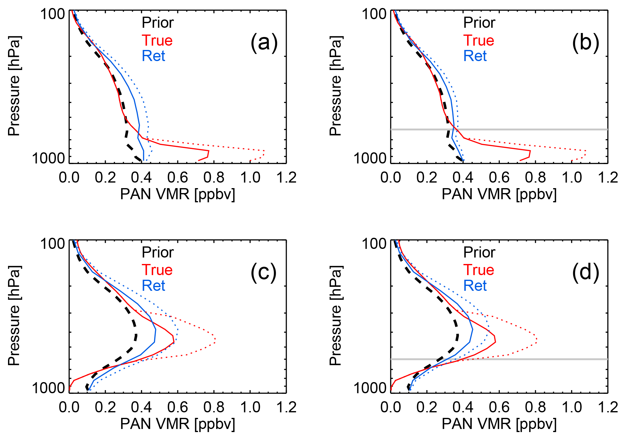
Figure 1 Simulated TES PAN retrievals for four different hypothetical conditions where the black dashed line shows the prior, the two red lines show two different true profiles, and the two blue lines show the retrieved profiles. The true profile exhibits a maximum in the volume mixing ratio (vmr) close to the surface in the upper panels (a and b), while the true profile peaks in the mid-troposphere in the lower panels (c and d). Panels on the left (a and c) show clear-sky retrievals while panels on the right (b and d) show retrievals where a cloud with effective optical depth of 0.7 is placed at 600 hPa (dotted line). Corresponding averaging kernels are provided in the Supplement.

At the time of this work, the v7 product was not yet available. The TES PAN retrievals shown here were processed using a prototype algorithm for the area and time periods of interest. The v7 PAN algorithm was built from this prototype, using the same state vector representation, microwindows, and prior constraints. The a priori profiles are based on GEOS-Chem simulations for the year 2008, with six possible prior profiles for any given month, as described in Payne et al. (2014). We have verified, using a subset of v7 data processed so far, that v7 retrievals are consistent with those from the prototype. On a single footprint basis, TES is capable of measuring elevated PAN (detection limit ∼ 0.2 ppbv) in the free troposphere, with an uncertainty of 30–50 % (Payne et al., 2014). In order to illustrate the characteristics of the retrievals, the four panels in Fig. 1 show simulated retrievals for different combinations of conditions. The true profiles in Fig. 1 are the profiles that were used to generate radiances and Jacobians for the purposes of the simulated retrievals shown in the figure. The true profile exhibits a maximum in the PAN mixing ratio close to the surface in the upper panels (a and b), while the true profile peaks in the mid-troposphere in the lower panels (c and d). In each of the profile plots, the black dashed line shows the prior, the two red lines show two different true profiles, and the two blue lines show the retrieved profiles. In order to demonstrate the reduction in lower tropospheric sensitivity associated with cloudy cases, panels on the right (b and d) show retrievals where a cloud with effective optical depth of 0.7 is placed at 600 hPa (dotted line). These can be directly compared with panels on the left (a and c), which show equivalent condition clear-sky retrievals. As discussed in Payne et al. (2014), the TES PAN retrievals do not provide information on the vertical variation of PAN. In all cases, the degrees of freedom for signal, or number of independent pieces of vertical information in the retrieval, is less than 1.0. This means that the shape of the retrieved result is always influenced by the shape of the prior (black dashed line), as can be seen in this figure, and the vertical distribution of PAN in each retrieval is uncertain. Figure 1 demonstrates the limitations in sensitivity of TES PAN measurements, which provide broader spatial and temporal coverage than in situ measurements, but with a compromise on sensitivity. However, the measurements can be used to validate models, provided the averaging kernel and prior are applied to model fields before comparison with the retrievals. The averaging kernels associated with the panels presented in Fig. 1 are provided in the Supplement (Fig. S1).

Figure 2 shows the July 2006–2009 tropospheric average PAN. Because of the lack of vertical information, we define the tropospheric average for a given retrieval as the average retrieved PAN between 800 hPa and the tropopause. The PAN spectral feature at 1140–1180 cm⁻¹ used for the TES retrievals coincides with the location of a silicate feature in surface emissivity spectra. For footprints where the spectra show strong evidence of this silicate feature in the surface emissivity (this can occur over rocky or sandy surfaces), TES PAN retrievals are not attempted. Of the 28 149 TES footprints processed for this work that fell over land, 3608 of them failed quality control. Spatially coherent regions of failed quality control show up as white patches in Fig. 2b. These regions are largely desert or mountainous regions. The same silicate feature is present in the presence of dust aerosol (e.g., DeSouza-Machado et al., 2006; Klüser et al., 2011; Capelle et al., 2014). The presence of dust aerosol could therefore also cause the retrieval to fail quality control or, for more subtle cases, could lead to low-biased PAN retrievals. Other reasons that may cause the TES PAN retrieval to fail quality control include poor fits to interferents, such as water vapor, within the PAN spectral range.

Figure 2 Average tropospheric PAN in retrievals (DOF > 0.6) during July 2006–July 2009 (a), and those retrievals averaged in a 2^∘ × 2^∘ grid (b). The white areas designate locations with less than five measurements during this period. The blue lines surround the regions included in the calculations in Figs. 4 and 5: 125–70^∘ W, 30–50^∘ N and 130–65^∘ W, 50–70^∘ N.

When all the existing TES data is gridded (Fig. 2b), there are several large patterns that emerge. (1) Average tropospheric PAN mixing ratios in the TES observations generally increase with latitude during the month of July over North America. (2) Average tropospheric PAN mixing ratios generally decrease from west to east. (3) As can be seen in later figures, there are relatively few retrievals per grid box over the southwestern US Though there are relatively few samples (∼ 5–20 per 2 × 2^∘ grid box), relatively high mixing ratios (0.6 ppbv) are observed over the Colorado Front Range. The increase with latitude has also been observed by TES over the eastern Pacific Ocean (Zhu et al., 2017), and GEOS-Chem furthermore produces a similar pattern in the mid-troposphere (Fischer et al., 2014). We are unaware of other work that has examined a longitudinal gradient in PAN over North America. PAN has recently been measured by in situ instruments in the Colorado Front Range, and mixing ratios exceeding 1 ppbv do occur in this region (Zaragoza et al., 2017).

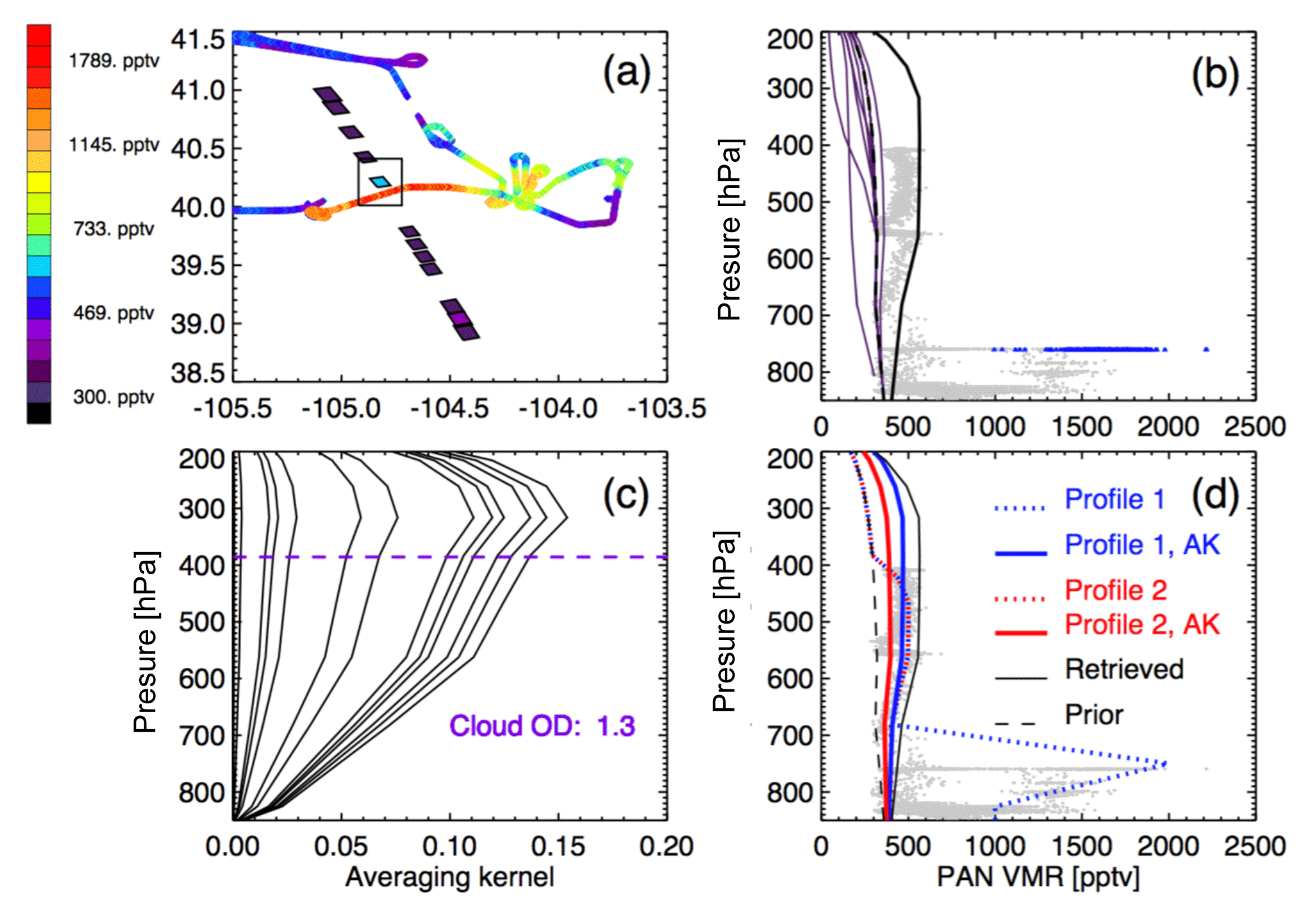
Figure 3 (a) Map showing FRAPPÉ aircraft and TES tropospheric average satellite observations of PAN over the Colorado Front Range on 29 July 2014. We define the tropospheric average for a given retrieval as the average retrieved PAN between 800 hPa and the tropopause. TES data show elevated PAN near the location where the aircraft data show highest values for that day. (b) All aircraft observations for 29 July 2014 are shown in grey. Blue points show aircraft data within 0.1^∘ longitude and 0.2^∘ latitude of the most elevated TES PAN observation. TES retrieved PAN profiles for 29 July 2014 are also shown. The elevated case is shown by the solid black line, while other cases are shown in purple solid lines. The black dashed line shows the TES a priori profile used in these retrievals. (c) TES averaging kernels for this case. The retrieval indicates that a high cloud is present, with optical depth 1.3, leading to reduced sensitivity below the cloud. (d) The blue dotted line shows a profile constructed to approximate the aircraft measurements, where PAN is highly elevated in the lower atmosphere. The blue solid line shows this same profile after smoothing with the TES prior and averaging kernel matrix for this scene. The red dotted line shows a hypothetical profile with no enhancement below 680 hPa, while the red solid line shows that same profile smoothed with the TES prior and averaging kernel.

The peak sensitivity for PAN is generally between 400 and 800 hPa (Payne et al., 2014), but a comparison between TES PAN transect observations coincident with Front Range Air Pollution and Photochemistry Éxperiment (FRAPPÉ) observations (Fig. 3) show that TES can have some degree of sensitivity to PAN in the boundary layer when boundary layer PAN is elevated. As an example, Fig. 3 presents in situ observations from a flight during FRAPPÉ made with a thermal dissociation–chemical ionization mass spectrometer (TD-CIMS) (Zheng et al., 2011). Mean PAN observed by the C-130 below 3 km during the field campaign was 481 pptv (Zaragoza et al., 2017). This particular day (29 July) was one of the four days identified by Zaragoza et al. (2017) with the highest surface PAN mixing ratios observed at the Boulder Atmospheric Observatory. The overlaid TES data in Fig. 3a (parallelograms) show an enhancement in the TES PAN (as shown by the TES observation highlighted by a black square) in the vicinity of aircraft measurements of highly elevated PAN values in the boundary layer, indicating that in this case TES is weakly sensitive to the elevated boundary layer values despite the presence of high clouds (dashed line Fig. 3c). Figure 3 also shows red and blue lines corresponding to the application of the averaging kernel for this case to hypothetical ”true” profiles with and without the enhancement in the boundary layer. The red and blue lines show that TES has some sensitivity to PAN located at altitudes below 800 hPa, but the retrieval places the additional PAN higher up in the atmosphere. While the difference between the red and the blue solid lines in Fig. 3d is small, it is non-zero indicating that TES has some sensitivity to the boundary layer enhancement in this case.

For the analysis presented below, we use PAN observations from TES over North America in July, from 2006 to 2009. We only include data with DOFS > 0.6. More specifically, this threshold value of DOF > 0.6 was chosen to be consistent with a signal-to-noise ratio (SNR) greater than 1 (Payne et al., 2014), and this criteria has been used in all the papers that have presented TES PAN data thus far (Jiang et al., 2016; Payne et al., 2017; Zhu et al., 2015, 2017). This conservative choice means that we are primarily basing our analysis on retrievals with high PAN. The mean (standard deviation) of the retrieved tropospheric average PAN mixing ratios for DOFS > 0.6 for the region shown in the figures presented here (125–70^∘ W, 30–50^∘ N and 130–65^∘ W, 50–70^∘ N) is 0.55 (0.93) ppbv. The impact of this choice can be seen when we compare the PAN distribution observed by TES under different conditions later in Sect. 3.2

2.2 NOAA Hazard Mapping System (HMS) smoke plume extent

We segregate the TES PAN retrievals by whether or not the TES footprint coincides with a smoke plume identified by the NOAA Hazard Mapping System (HMS). NOAA HMS is an interactive satellite image and graphics system developed by the National Environmental Satellite, Data, and Information Service (NESDIS). Using satellite imagery, trained analysts identify the geographic extent of smoke plumes in the atmospheric column over North America (Rolph et al., 2009; Ruminski et al., 2006). Visible-band geostationary (∼ 15 min refresh rate) imagery, occasionally assisted by infrared imagery, is used to detect smoke plumes in the atmospheric column (Ruminski et al., 2006); because smoke plumes are primarily identified with visible imagery, the analyzed smoke plume extent is only representative of local daylight hours.

Plumes are analyzed multiple times on a given day and can be nested. For this work all overlapping plumes (either nested or analyzed at different times) are merged into a single plume. This dataset does not contain information about the vertical location or depth of smoke in the atmospheric column. As discussed in Brey et al. (2018), the number and extent of smoke plumes in this HMS dataset is a conservative estimate. In particular, it becomes challenging to identify smoke as it dilutes during transport or mixes with anthropogenic haze. Thus our estimate of the number of PAN retrievals impacted by smoke may be a lower bound. For this work, we follow the overlap methods described in Brey et al. (2018). We matched all TES PAN retrievals based on UTC day. This means that overnight retrievals are paired with the plume from the prior day. As discussed in Brey et al. (2018), most of the large wildfire plumes occurring in July over the western US are very large and last several days. So we would expect that pairing the overnight retrievals with the plume from the prior day (i.e., matching based only on UTC day) is not likely to change our results, and that is the case. We have repeated all our calculations using only the daytime retrievals, and the choice to use all the retrievals does not change the results.

Figure 4 Panels (a) through (d): PAN TES retrievals with DOF > 0.6 co-located with NOAA Hazard Mapping System smoke polygons (red), and PAN TES retrievals with DOF > 0.6 not co-located with NOAA Hazard Mapping System smoke polygons (grey). The black dots indicate PAN TES retrievals with DOF > 0.6 during times with no NOAA HMS data. The blue lines surround the regions included in the distributions shown in Fig. 5: 125–70^∘ W, 30–50^∘ N and 130–65^∘ W, 50–70^∘ N. (e) Percent of TES PAN retrievals overlapping HMS smoke plume polygons for July 2006–2009. (f) Percent of TES PAN retrievals overlapping HMS smoke plume polygons for May–September 2006. In panels (e) and (f) the red bars indicate the percentage of all retrievals overlapping smoke plumes, and the striped bars indicate the percentage of daytime retrievals overlapping smoke plumes. Pairing was done using the matching UTC day.

2.3 HYSPLIT trajectories

As part of a case study presented in Sect. 3.3, we use the Hybrid Single-Particle Lagrangian Integrated Trajectory (HYSPLIT) model (Draxler and Hess, 1998) (http://ready.arl.noaa.gov/HYSPLIT.php) to simulate the air mass history of a subset of TES PAN retrievals associated with relatively fresh (0–2 days of atmospheric processing) smoke. HYSPLIT has been used extensively to model the transport of smoke (e.g., Stein et al., 2015; Brey et al., 2018). For this application, the HYSPLIT model is driven by global meteorological data from the Global Data Assimilation System (GDAS) archive (ftp://arlftp.arlhq.noaa.gov/pub/archives/gdas1). GDAS has a time step of 3 h, horizontal grid spacing of 1^∘ latitude by 1^∘ longitude (∼ 120 km), and 23 pressure surfaces between 1000 and 20 hPa (Kanamitsu, 1989). We initialized 5-day backward trajectories for set of single TES retrievals at the retrieval times and locations. In the case study in Sect. 3.3 we used trajectories initialized at 2, 4 and 6 km a.g.l. (above ground level). As the vertical distribution of PAN in each retrieval is uncertain (Sect. 2.1), we calculated backward trajectories using these three altitudes to test the sensitivity of our results to the choice of initialization altitude.

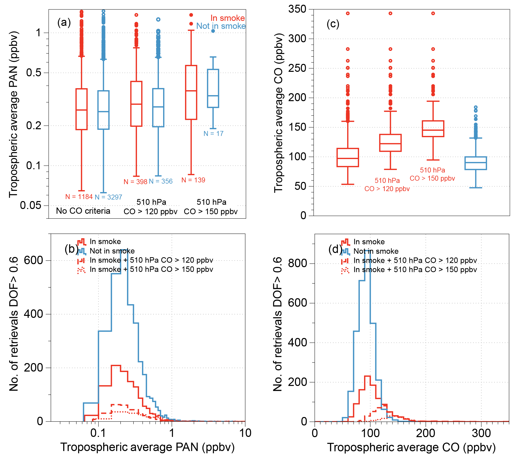
Figure 5 (a) Box plots of July 2006–2009 North American TES PAN retrievals colored by whether they overlap HMS smoke plume polygons. Red (“In Smoke”) designates overlap; blue-grey designates non-overlapping retrievals. The left set of box plots include all the retrievals with DOF > 0.6, the center set of box plots only include retrievals with 510 hPa TES CO > 120 ppbv, and the right set of box plots only include retrievals with 510 hPa TES CO > 150 ppbv. (b) Histograms of July 2006–2009 TES PAN retrievals. (c) Box plots of July 2006–2009 TES CO retrievals coincident with the TES PAN retrievals subset by 510 hPa TES CO. (d) Histograms of July 2006–2009 TES CO retrievals coincident with the TES PAN retrievals. The box plots display the interquartile range for each subset and the dots represent outliers.

3 Results

3.1 North American TES PAN retrievals associated with smoke

The first four panels of Fig. 4 show the spatial distribution of TES PAN retrievals over the US and southern Canada for the month of July 2006 to 2009. All retrievals plotted in this figure have DOF > 0.6. The retrievals are colored red when they fall within a NOAA HMA smoke plume. A large fraction of the TES retrievals (15–32 %) during this month overlap smoke plumes; the largest percentage of retrievals associated with smoke occurred in July 2008 (32 %), though this year does not display a high percentage of detection compared to other years and the average tropospheric PAN measured by TES is not larger than other years (Fig. S2). Of all the retrievals attempted in July 2006 to July 2009, 18 % were associated with smoke. We expect a higher fraction of overlap in the subset of data with DOF > 0.6 (28 %). This threshold value of DOF > 0.6 is consistent with a signal-to-noise ratio greater than 1 (Payne et al. 2014), and this subset of data only reflects conditions with elevated PAN in the atmospheric column. The number of major wildfires over the US has large seasonal and interannual variability (Brey et al., 2018). Wildfires in summer 2008 were particularly intense over California associated with record-breaking lightning and aggravated drought. Fig. 4c shows a cluster of TES PAN retrievals over California associated with this smoke. The dense smoke, which spread substantially downwind, was sampled from the NASA DC-8 aircraft as part of the Arctic Research of the Composition of the Troposphere from Aircraft and Satellites (ARCTAS-CARB) campaign (Hecobian et al., 2011; Singh et al., 2010, 2012), and we show this data in Sect. 3.3. Elevated smoke was also observed at surface sites downwind throughout the month of July (Gyawali et al., 2009). As part of ARCTAS-B, Alvarado et al. (2010) also documented major PAN enhancements in fresh wildfire plumes sampled over Canada during July 2008. July 2008 was additionally associated with special observations from TES, providing a relatively high number of attempted retrievals this month (red line in Fig. S2). Figure 4f presents the seasonal transition for 2006 in smoke-plume polygon overlap from late spring (May) to early autumn (September). During this example year, the percentage of TES PAN retrievals with DOF > 0.6 associated with smoke peaked in July (20 %), but Fig. 4e suggests that this was not a notably high percentage of smoke-impacted retrievals. A much higher percentage of DOF > 0.6 retrievals were smoke-impacted in July 2008.

Panels a and b of Fig. 5 show the distribution of tropospheric average TES PAN in the subset of retrievals overlapping HMS smoke plume polygons in July 2006–2009. The distributions of tropospheric PAN in the subset of retrievals with DOF > 0.6 is not different between the in-smoke cases (leftmost red box plot in Fig. 5a) and the not-in-smoke cases (blue-grey box plot in Fig. 5a). The choice to only include data with DOFS > 0.6, pushes the median tropospheric average PAN substantially higher than using all the available TES data. Thus the percent of retrievals impacted by smoke shown in Fig. 4 reflects only situations with substantially elevated PAN in the atmospheric column. Imposing an additional cloud optical depth filter does not substantially change the distribution of tropospheric average PAN (see Fig. S4). The other two red distributions in Fig. 5a reflect additional criteria designed to ensure that the PAN associated with smoke in the atmospheric column exists in the free troposphere where we expect TES to be most sensitive. We show the PAN distribution for in-smoke cases that also coincide with TES 510 hPa CO > 120 ppbv and TES 510 hPa CO > 150 ppbv. As discussed further in Sect. 3.3, background CO in July in the northern mid-latitudes is expected to be ∼ 85 ppbv. Both criteria (510 hPa CO > 120 ppbv or 510 hPa CO > 150 ppbv) represent conservative indicators of smoke in the free troposphere. The latter subset is shown because this designation has been used previously (Alvarado et al., 2011), and we use this subset in our calculation of enhancement ratios in Sect. 3.3. We have done a similar CO-based sub-setting for the retrievals that are not located within HMS smoke polygons. However, there are only 17 retrievals located outside HMS smoke polygons that have TES 510 hPa CO > 150 ppbv. Fires primarily drive CO enhancements of this magnitude. While there is a suggestion that PAN is higher in smoke-impacted plumes in Fig. 5a, this is not significant and the suggested differences are likely an underestimate. The in-smoke cases are a conservative estimate of smoke in the atmospheric column. The largest uncertainty in the HMS-based smoke designation is at the edges of the HMS plumes. As discussed in Brey et al. (2018), as smoke plumes dilute with age they become more difficult to visibly identify and to distinguish from anthropogenic pollution. This means that there are likely smoke-impacted retrievals that we have misclassified as smoke-free.

Figure 5c and d present the distribution of tropospheric mean CO associated with the successful PAN measurements. There is higher CO associated with TES retrievals that overlap HMS smoke polygons (median = 100 ppbv versus 92 ppbv for both day and night retrievals), and the upper tail of the CO distribution includes retrievals with tropospheric average CO above 200 ppbv. The difference in CO distributions in and out of smoke provides confidence in the use of the HMS smoke product as a smoke-impact filter. The tropospheric average CO distributions are shown for reference because we combine tropospheric average CO with tropospheric average PAN to calculate PAN enhancement ratios in Sect. 3.3. There are several other factors that may also contribute to the patterns shown in Fig. 5 that are worth noting. In general, TES is more sensitive to CO than PAN in the lowermost atmosphere, and the HMS smoke product, which contains no vertical information, includes smoke plumes near the surface and higher in the column. Though the sensitivity to clouds appears to be modest in our data, the TES CO retrievals are even less sensitive overall to the presence of cloud than the TES PAN retrievals. Third, many of the smoke-impacted TES retrievals are located substantially downwind of the source fires. PAN has a substantially shorter lifetime than CO in the warm lower atmosphere in summer.

3.2 July 2007 case study

TES observations allow measurements of smoke plumes over North America at various ages, even in the same day. Figure 6 shows the spatial distribution of TES retrievals with DOF > 0.6 over the US and southern Canada for the month of July 2006 to 2009 that overlapped HMS smoke plume polygons. These points are the red colored retrieval locations in Fig. 4, but here they have been colored by the day of the month. The filled dots represent points where TES 510 hPa CO > 150 ppbv, and these are the points used to calculate PAN enhancement ratios in Sect. 3.3. The presence of same colored dots demonstrate that wide swaths of North America can have smoke located somewhere in the atmospheric column on a given day, and that the smoke is associated with elevated PAN (> 200 pptv) in the atmospheric column. As discussed in Brey et al. (2018), smoke plumes vary substantially in size. Small plumes cover < 100 km² and smoke plumes from major fire complexes can spread over several western states or entire Canadian provinces. For example, Fig. 6 shows elevated PAN both directly over and east of Hudson Bay in late July 2008 associated with fires in northern Saskatchewan.

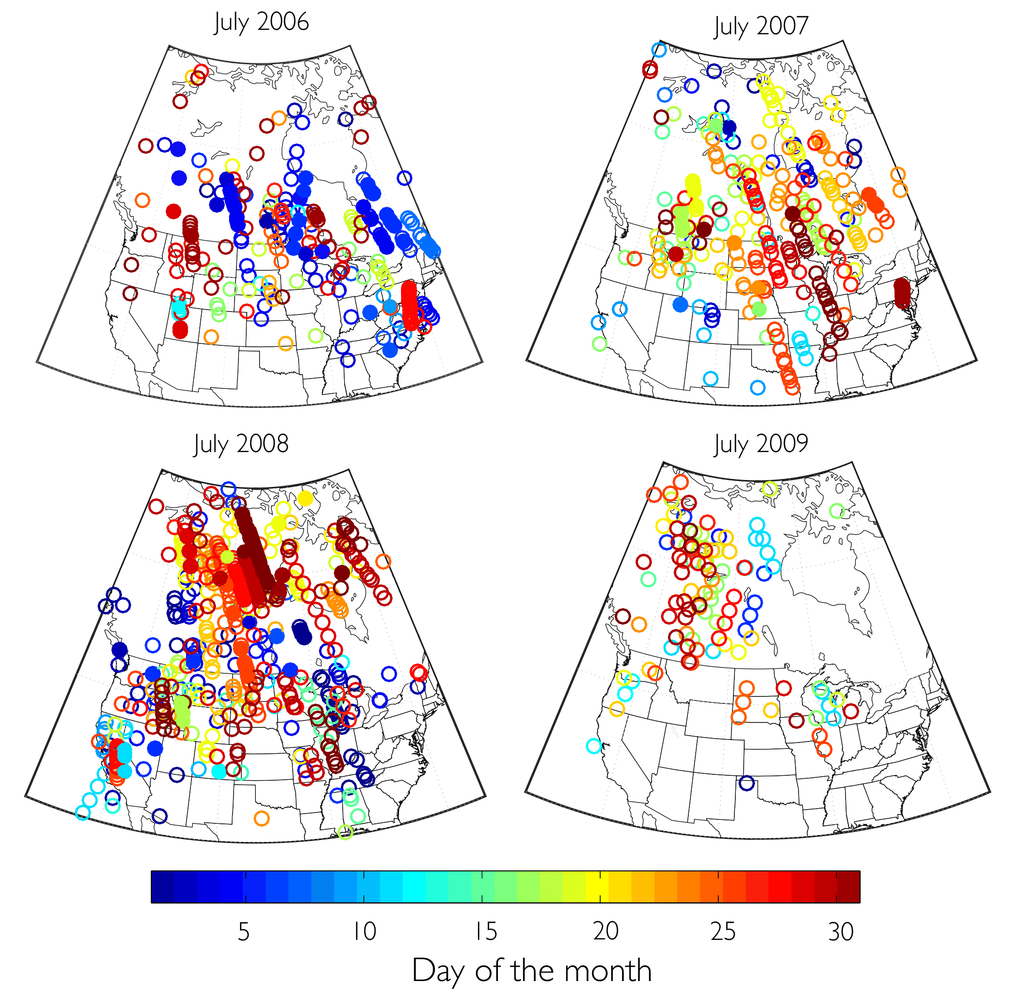
Figure 6 Successful TES PAN retrievals overlapping NOAA HMS smoke polygons for July 2006 to July 2009 colored by the day of the month. Filled circles denote the set of retrievals that also coincide with 510 hPa CO greater than 150 ppbv. This set of points is used to calculated PAN enhancement ratios relative to CO in Fig. 8.

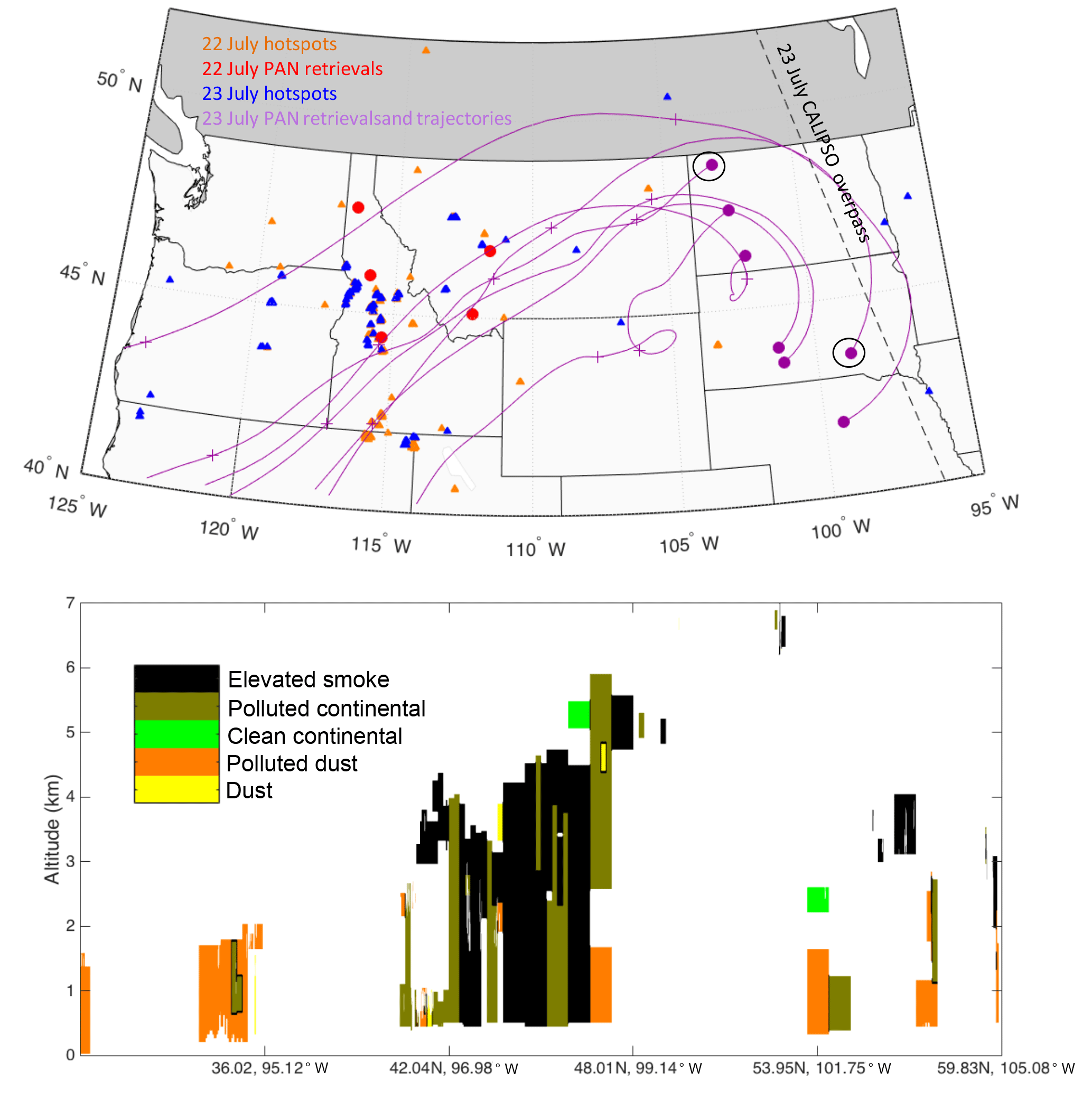
Figure 7 Top panel: case study of TES PAN retrievals overlapping HMS smoke polygons 22–23 July 2007. Orange triangles represent FIRMS MODIS hotspots for 22 July (Product MCD14ML; https://earthdata.nasa.gov/earth-observation-data/near-real-time/firms). Blue triangles represent FIRMS MODIS hotspots for 23 July. Red circles indicate TES PAN retrievals on 22 July, and purple circles represent TES PAN retrievals on 23 July. We have circled the two retrievals in this set with 510 hPa CO greater than 150 ppbv. The PAN enhancement ratios for these points are noted in Fig. 7. The purple lines signify 5 day HYSPLIT backward trajectories initialized at each TES retrieval at 4 km. The purple “+” signifies 24 h of transport time on the 4 km trajectories. The black dashed line shows the location of the CALIPSO swath shown in the lower panel. Lower panel: CALIPSO aerosol subtype observed on 23 July 2007. CALIPSO Science Team (2016), CALIPSO/CALIOP Level 2, Vertical Feature Mask Data, version 4.10, Hampton, VA, USA: NASA Atmospheric Science Data Center (ASDC), accessed by Emily V. Fischer at https://doi.org/10.5067/CALIOP/CALIPSO/LID_L2_VFM-Standard-V4-10.

Next we present a case study of fires in Idaho and Montana during July 2007 that connects PAN enhancements associated with HMS smoke plumes to regions impacted by fires, indicating that the TES sensitivity is often sufficient to measure elevated PAN several days downwind of a fire. Figure 7 presents the locations of TES retrievals with elevated (DOF > 0.6) PAN on 22 and 23 July 2007, red and purple dots respectively, along with FIRMS MODIS hotspots (Giglio et al., 2003, 2006) on those two dates. The TES PAN retrievals are located almost directly over active fires in Idaho on 22 July, but this does not absolutely ensure that the PAN is from fresh smoke. As discussed in Payne et al. (2014), TES is most sensitive to PAN in the mid-troposphere, and we do not have injection height information for these specific fires. The TES PAN retrievals on 23 July (located over rural areas in North and South Dakota) are not located directly over active fires, but they do overlap HMS smoke polygons. The purple lines show HYSPLIT backward trajectories initialized from 4 km at the locations of the retrievals on 23 July. The trajectories show that the major fire complexes in Idaho and Montana likely contributed to the smoke observed by TES on 23 July (purple dots). If so, this smoke was approximately 1–2 days old at the time of the retrieval. The trajectories show that the smoke observed over South Dakota is likely older (2–3 days of atmospheric aging). We initialize the trajectories from various heights (2, 4, and 6 km) because the TES PAN retrievals offer no vertical information, and all these trajectories are plotted in Fig. S3. The smoke filled a relatively thick layer based on available CALIPSO data. A CALIPSO overpass on 23 July 2007 (lower panel of Fig. 7) shows an aerosol layer identified largely as elevated smoke extending from the surface to ∼ 5 km over this region.

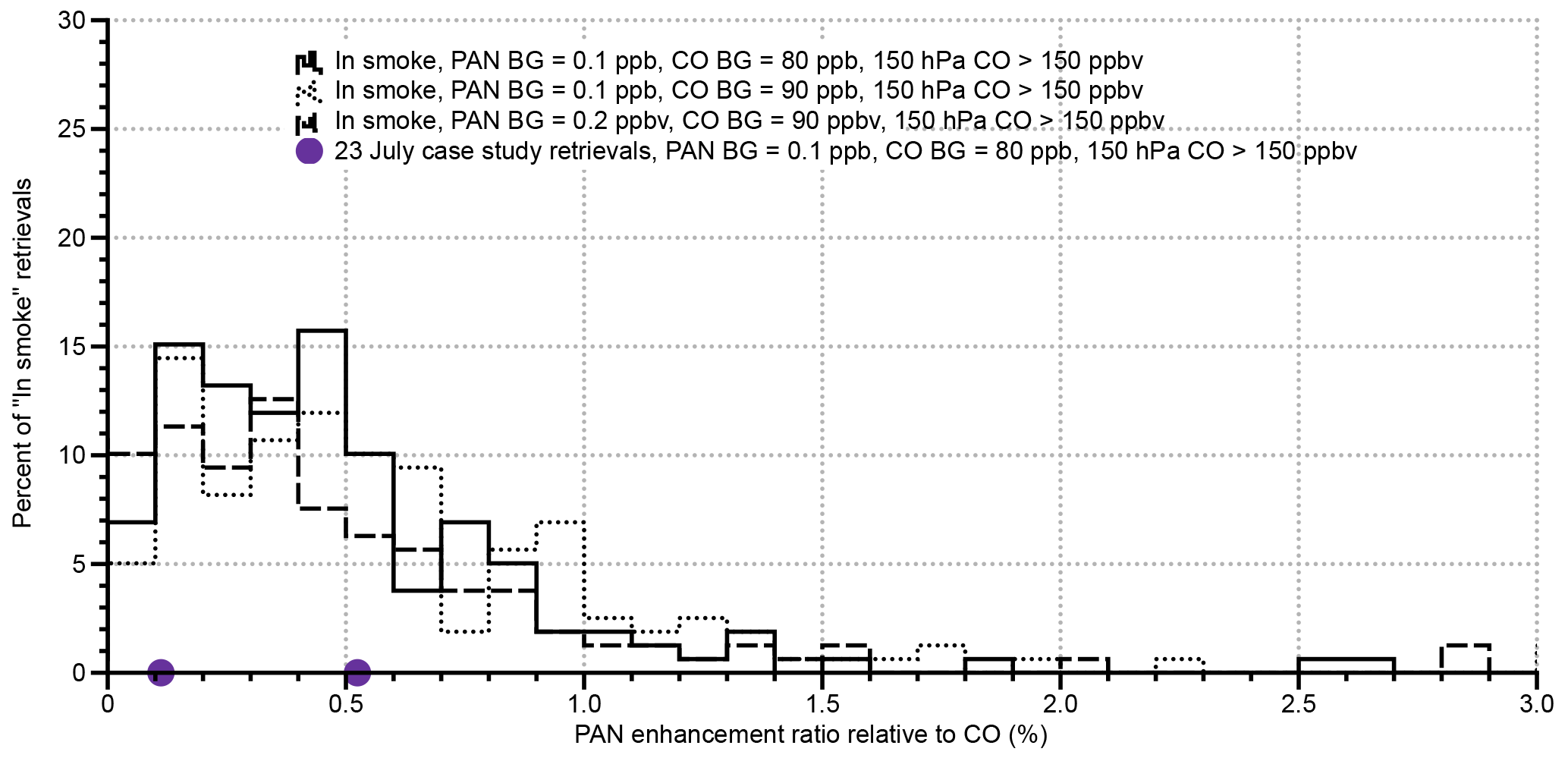
Figure 8 Histogram of estimated PAN enhancement ratios based on tropospheric mean PAN and CO from July 2006–2009 North American TES PAN retrievals overlapping HMS smoke plume polygons. The solid black line represents enhancement ratios calculated using an assumed PAN background of 0.1 ppbv with an assumed CO background of 80 ppbv. The dotted black line represents enhancement ratios calculated using an assumed PAN background of 0.1 ppbv with an assumed CO background of 90 ppbv. These specific enhancement ratios were calculated using an assumed CO background of 80 ppbv, similar to the solid black line. The dashed line represents enhancement ratios calculated using a significantly higher assumed PAN background of 0.2 ppbv with an assumed CO background of 90 ppbv. In all cases, negative values are not shown. The purple dots are the enhancement ratios for the two circled retrievals on 23 July 2007 plotted in Fig. 7 associated with transported smoke.

3.3 PAN enhancements in North American biomass burning plumes

Enhancement ratios relative to CO or another tracer (e.g., acetonitrile for biomass burning specifically) are a common way to characterize the composition of pollution plumes (Yokelson et al., 2013). Enhancement ratios are calculated from samples made from within and outside a given plume (i.e., background air). This section presents enhancement ratios calculated from TES PAN retrievals located within smoke plumes. We show that the tropospheric PAN enhancement ratios from TES fall within the range of relevant aircraft measurements over North America. We also show that there are many pitfalls associated with using enhancement ratios as observed from TES to study the evolution of PAN in the smoke plumes we have identified here.

Equation (4) indicates how the enhancement ratio of PAN relative to CO is calculated here.

$$\begin{array}{ll}\text{(4)}& {\displaystyle }& {\displaystyle }{\mathrm{PAN}}_{\mathrm{ER}}={\displaystyle }& {\displaystyle }({\mathrm{PAN}}_{\mathrm{plume}}-{\mathrm{PAN}}_{\mathrm{background}})/({\mathrm{CO}}_{\mathrm{plume}}-{\mathrm{CO}}_{\mathrm{background}})\end{array}$$

Figure 8 presents a histogram of PAN enhancement ratios in the subset of retrievals that overlap HMS smoke polygons and are also likely to have elevated PAN and CO in the free troposphere (TES CO > 150 hPa). The purple dots designate the two retrievals shown in Fig. 7 that meet these strict criteria. PAN enhancement ratios were estimated using tropospheric average PAN and tropospheric average CO. We performed this calculation using Eq. (4) and a CO background of 80 and 90 ppbv. Background CO in the Northern Hemisphere is generally between 80 and 90 ppbv (e.g., Parrish et al., 1991) with significant year-to-year variability largely driven by boreal forest fire emissions (Wotawa et al., 2001). Thus the lower mixing ratio (80 ppbv) is closer to estimates of background CO in the Northern Hemisphere. The upper mixing ratio (90 ppbv) reflects the median tropospheric average CO (91 ppbv) in the PAN TES retrievals not overlapping HMS smoke polygons (blue-grey points in Fig. 4). Though we repeated this calculation with various assumptions of background CO mixing ratios, this choice does not impact the major key point we draw from Fig. 8. Even with our conservative CO criteria applied, the TES PAN data offer the opportunity to calculate tropospheric average PAN enhancements relative to CO for a large number of smoke samples (N=159) over a variety of regions and distances downwind from fires. The median PAN enhancement ratio relative to CO calculated using a background PAN mixing ratio of 0.1 ppbv and a background CO mixing ratios of 90 ppbv is 0.43 %. When we assume a higher PAN background mixing ratio of 0.2 ppbv with this background CO mixing ratio, the median PAN enhancement ratio from the TES data is 0.29 %. As we show next, these values are similar to that reported from in situ measurements.

We have not been able to identify a case study where the TES data can be used to examine the evolution of the enhancement ratio of PAN relative to CO in a plume. Restricting ourselves to the conservative criteria of 510 hPa CO > 150 ppbv severely reduces the sample size (from 1151 to 159). In addition, the 5 km × 8 km footprint of TES combined with the lack of vertical sensitivity makes it difficult to establish the age of the smoke contributing to the enhanced PAN and CO. There could be multiple layers of smoke in the column, of various ages. Tracking plumes with aircraft allows for a more precise determination of plume age. In addition, PAN does not simply dilute proportionally to CO because its dissociation is also a function of temperature, which also depends on altitude.

We compare the TES column PAN enhancement ratios to enhancement ratios of PAN relative to CO observed during July 2008 during the ARCTAS/CARB field campaign (Hecobian et al., 2011). Smoke identification within the aircraft dataset is discussed in detail in Hecobian et al. (2011) and not repeated here. Alvarado et al. (2010) report mean PAN enhancement ratios for boreal plumes using this same dataset. They report enhancement ratios of 0.34 ± 0.35 % (range = 0.09 to 1.43 %) for fresh plumes and 0.28 ± 0.36 % (range = 0.16 to 0.68 %) for old plumes. In Alvarado et al. (2010), fresh plumes were designated as those where propene was correlated with CO, and aged plumes were designated as plumes where CO was correlated with more long-lived species, like butane, benzene, and propane. The enhancement ratios were calculated using aircraft data from plume crossings using the average within-plume PAN and CO mixing ratios and assuming background mixing ratios equal to the 25th percentile of all measurements in the boundary layer (140 ppbv for CO and 180 pptv for PAN). To calculate the enhancement ratios presented in Fig. 9, we used the 25th percentile for each trace gas for each day. For simplicity, we used observations at all altitudes, not just boundary layer points. Figure 9 shows that there is a range of in situ enhancement ratios. Similar to the tropospheric average enhancement ratio from TES, the majority of these enhancement ratios fall below 1 %. There are retrievals with PAN enhancement ratios greater than 1 %, but the number of these depends on the assumed background PAN used in the calculation. The appropriate value to use is difficult to determine from the TES data alone, which is why a range of estimates is presented in Fig. 8. Figure 9 presents enhancement ratios calculated from in situ measurements. This data shows that there is a higher median enhancement for plumes from fires in the northwestern US, than the boreal plumes, though there are vastly different numbers of samples.

Figure 9 Histogram of estimated PAN enhancement ratios based on in situ measurements of fire plumes described in Hecobian et al. (2011) from the ARCTAS campaign. Enhancement ratios were calculated using the 25th percentile for each trace gas during the corresponding flight day. These ratios were calculated using the 1 min merged data.

A second chance for a qualitative comparison of PAN enhancement ratios in smoke plumes is presented in Briggs et al. (2016); summertime observations of 23 different plumes from the Mount Bachelor Observatory indicate PAN enhancement ratios of 1.46–6.25 pptv ppbv⁻¹ (0.146–0.625 %). This range overlaps with the majority of the column average enhancement ratios from TES. All of the plumes identified in Briggs et al. (2016) were from fires in northern California or southeastern and central Oregon, so they differ from the fires intercepted during ARCTAS.

4 Conclusions

We present the first detailed analysis of TES PAN measurements over North America. Recent aircraft observations over Colorado offer the most direct overlap of the TES PAN product with in situ aircraft observations to date. This comparison indicates that TES can be sensitive to PAN in the boundary layer when PAN in the boundary layer is elevated, though peak sensitivity is in the free troposphere. We use a period with a large number of TES PAN observations (2006–2009) to investigate the contribution of fire smoke to elevated PAN over North America in July. This type of multi-year synthesis is not possible with any other observational dataset, and demonstrates how satellite measurements of PAN can be used to frame new questions that cannot be answered with existing in situ measurements.

1. We segregate and examine the abundance of tropospheric average PAN relative to CO in TES retrievals located within smoke plumes identified by the NOAA Hazard Mapping System (HMS). We find that a large fraction of the TES retrievals (15–32 %) during the month of July overlap smoke plumes during the period 2006–2009, while the largest percentage of retrievals associated with smoke occurred in July 2008 (32 %). Tropospheric average CO is clearly enhanced in retrievals impacted by smoke, but a difference in PAN between smoke-free and smoke-impacted retrievals is insignificant.

2. We compare the tropospheric average PAN enhancement relative to CO in smoke-impacted samples and find that our satellite-based estimates largely fall within the range of enhancement ratios that have been observed from recent aircraft and surface campaigns over western North America. While in situ measurements represent samples from a select number of plumes, the satellite measurements offer more samples of different plumes and observations over regions and time periods that have not been sampled by aircraft.

3. We use a case study to illustrate that PAN enhancements associated with HMS smoke plumes can be connected to regions impacted by fires, indicating that the TES sensitivity is often sufficient to measure elevated PAN several days downwind of a fire.

4. Case studies of specific smoke events do not show a systematic pattern in PAN enhancements relative to CO as a function of distance downwind from presumed source fires. We also do not observe any consistent evolution in the PAN enhancement ratio when this calculation is done using the tropospheric maximum PAN and CO from the TES retrievals, rather than the tropospheric averages. The TES PAN data are not useful in this context because of large limitations associated with evaluating smoke age within the TES data.

PAN is considered to be the most important reservoir for NO_x in the troposphere, and it plays a critical role in the redistribution of NO_x to remote regions. The work presented here highlights the importance of fires as a source of PAN over North America in summer. It also shows that TES measurements of PAN can be used to complement limited in situ measurements of PAN. The apparent significant contribution of fires to elevated PAN plumes over North America underscores the importance of investigating PAN production in smoke to ultimately determine the best way to incorporate the rapid chemistry that produces PAN into chemical transport models that are used to predict background O₃ and exceptional O₃ events.