the Creative Commons Attribution 4.0 License.
the Creative Commons Attribution 4.0 License.
 | 19 Apr 2018
The effect of South American biomass burning aerosol emissions on the regional climate
Gillian D. Thornhill
Claire L. Ryder
Eleanor J. Highwood
Len C. Shaffrey
Ben T. Johnson
The impact of biomass burning aerosol (BBA) on the regional climate in South America is assessed using 30-year simulations with a global atmosphere-only configuration of the Met Office Unified Model. We compare two simulations of high and low emissions of biomass burning aerosol based on realistic interannual variability. The aerosol scheme in the model has hygroscopic growth and optical properties for BBA informed by recent observations, including those from the recent South American Biomass Burning Analysis (SAMBBA) intensive aircraft observations made during September 2012. We find that the difference in the September (peak biomass emissions month) BBA optical depth between a simulation with high emissions and a simulation with low emissions corresponds well to the difference in the BBA emissions between the two simulations, with a 71.6 % reduction from high to low emissions for both the BBA emissions and the BB AOD in the region with maximum emissions (defined by a box of extent 5–25∘ S, 40–70∘ W, used for calculating mean values given below). The cloud cover at all altitudes in the region of greatest BBA difference is reduced as a result of the semi-direct effect, by heating of the atmosphere by the BBA and changes in the atmospheric stability and surface fluxes. Within the BBA layer the cloud is reduced by burn-off, while the higher cloud changes appear to be responding to stability changes. The boundary layer is reduced in height and stabilized by increased BBA, resulting in reduced deep convection and reduced cloud cover at heights of 9–14 km, above the layer of BBA. Despite the decrease in cloud fraction, September downwelling clear-sky and all-sky shortwave radiation at the surface is reduced for higher emissions by 13.77 ± 0.39 W m−2 (clear-sky) and 7.37 ± 2.29 W m−2 (all-sky), whilst the upwelling shortwave radiation at the top of atmosphere is increased in clear sky by 3.32 ± 0.09 W m−2, but decreased by W m−2 when cloud changes are included. Shortwave heating rates increase in the aerosol layer by 18 % in the high emissions case. The mean surface temperature is reduced by 0.14 ± 0.24 ∘C and mean precipitation is reduced by 14.5 % in the peak biomass region due to both changes in cloud cover and cloud microphysical properties. If the increase in BBA occurs in a particularly dry year, the resulting reduction in precipitation may exacerbate the drought. The position of the South Atlantic high pressure is slightly altered by the presence of increased BBA, and the strength of the southward low-level jet to the east of the Andes is increased. There is some evidence that some impacts of increased BBA persist through the transition into the monsoon, particularly in precipitation, but the differences are only statistically significant in some small regions in November. This study therefore provides an insight into how variability in deforestation, realized through variability in biomass burning emissions, may contribute to the South American climate, and consequently on the possible impacts of future changes in BBA emissions.
- Article
(8019 KB) - Full-text XML
-
Supplement
(1017 KB) - BibTeX
- EndNote


Land management practices in South America designed to increase available land for agriculture and pasture and increasing urbanization have resulted in deforestation altering an estimated 18 % of the original forest area (Artaxo et al., 2013). The biomass burning aerosol (BBA) emissions from fires tend to be largest where there is rapid deforestation (e.g. south-east Amazonia) and lowest in the tropical forests in central Amazonia where the density of the forest canopy and larger amounts of moisture generally prevent fires, and areas where the fires occur in already cleared agricultural and pastoral land tend to have lower fuel loads and result in reduced fire emission per unit area compared to areas of rapid deforestation (Reddington et al., 2015; DeFries et al., 2008). Reddington et al. (2015) show that there is a clear positive relationship between deforestation, BBA emissions and aerosol optical depth (AOD).
The biomass burning aerosols absorb and scatter radiation, and affect the surface fluxes and atmospheric stability. BBA also increase the concentration of cloud condensation nuclei (CCN) affecting the formation and lifetime of clouds (Koren et al., 2008; Sena et al., 2013; Koch and Del Genio, 2010). They consist largely of carbonaceous material, with a relatively low single scattering albedo (SSA) indicating they are more absorbing than, for example, sulfate aerosols. There is a direct effect on the radiative budget from both scattering and absorption (Charlson et al., 1992), as well as the absorption results in atmospheric heating which, together with the reduced solar radiation reaching the surface, changes the stability of the atmosphere. Heating of the atmosphere where aerosols and clouds are co-located (in altitude) is predicted to result in cloud cover changes as cloud “burns off” or is prevented from forming due to the stabilization of the atmospheric profile. This process has been termed the semi-direct effect (Hansen et al., 1997; Koren et al., 2008), although other studies have pointed out that the semi-direct effect could have the opposite tendency, for instance if increased atmospheric stability favours the persistence of stratocumulus (Johnson et al., 2004). The overall aerosol–cloud interaction is complex, however, with the semi-direct effect depending on the relative heights of the aerosol and the clouds, the type of cloud and the regional dynamics, e.g. convergent or divergent flow (Koch and Del Genio, 2010). The particles of smoke are also predicted to act as cloud condensation nuclei (Spracklen et al., 2011), changing the size and number of cloud droplets and resulting in changes to the reflectivity and lifetime of the clouds, referred to as the indirect effect (Twomey, 1974; Albrecht, 1989). Effects of BBA on convection and cloud formation characteristics can result in changes in precipitation (Gonçalves et al., 2015), which in turn will change hydrological processes (Koren et al., 2004). Furthermore, changes in the proportions of direct and diffuse radiation at the surface will affect photosynthesis and net primary productivity (Rap et al., 2015). Koren et al. (2008) investigated the effect of BBA on cloud formation and lifetime and suggested that the stabilization of the lower atmosphere, and the reduction in fluxes from the surface, can inhibit the formation of high and deep convective clouds, despite the possible destabilization of the higher atmosphere due to the increased heating of the atmosphere at lower levels. This effect is dependent on the initial cloud cover fraction, however, as a lower initial cloud cover permits more solar absorption and increases the aerosol heating effects. The BB AOD is also a factor, with the suggestion that at low (high) BB AOD, the indirect effect is more (less) important than the semi-direct effect (Ten Hoeve et al., 2012). Feingold et al. (2005) used large eddy simulation modelling for biomass burning (BB) in Amazonia to show that where the BBA was at the cloud formation layer, this would act to reduce cloud fraction, but BBA at lower levels may tend to either increase or decrease cloudiness. However, they also found that surface sensible and latent heat fluxes are sufficient in themselves to reduce cloudiness.
Assessing the relative importance of these various effects is crucial to understanding the overall impact of BBA on the regional climate, but there is some uncertainty in how to treat and describe aerosol properties in climate models that can affect the results of such studies. Our approach uses new observations of aerosol optical properties, and compares two different scenarios, a high-BBA-emission experiment with a low-BBA-emission experiment, so that we are considering changes due to decadal timescale variability in emissions (rather than a comparison of the regional climate with BBA to one without BBA). This provides some insight into how changes in deforestation practices, which are positively related to BBA emissions and BBA AOD (Reddington et al., 2015), and the resulting changes in the characteristics of the BBA over time might affect the regional climate.
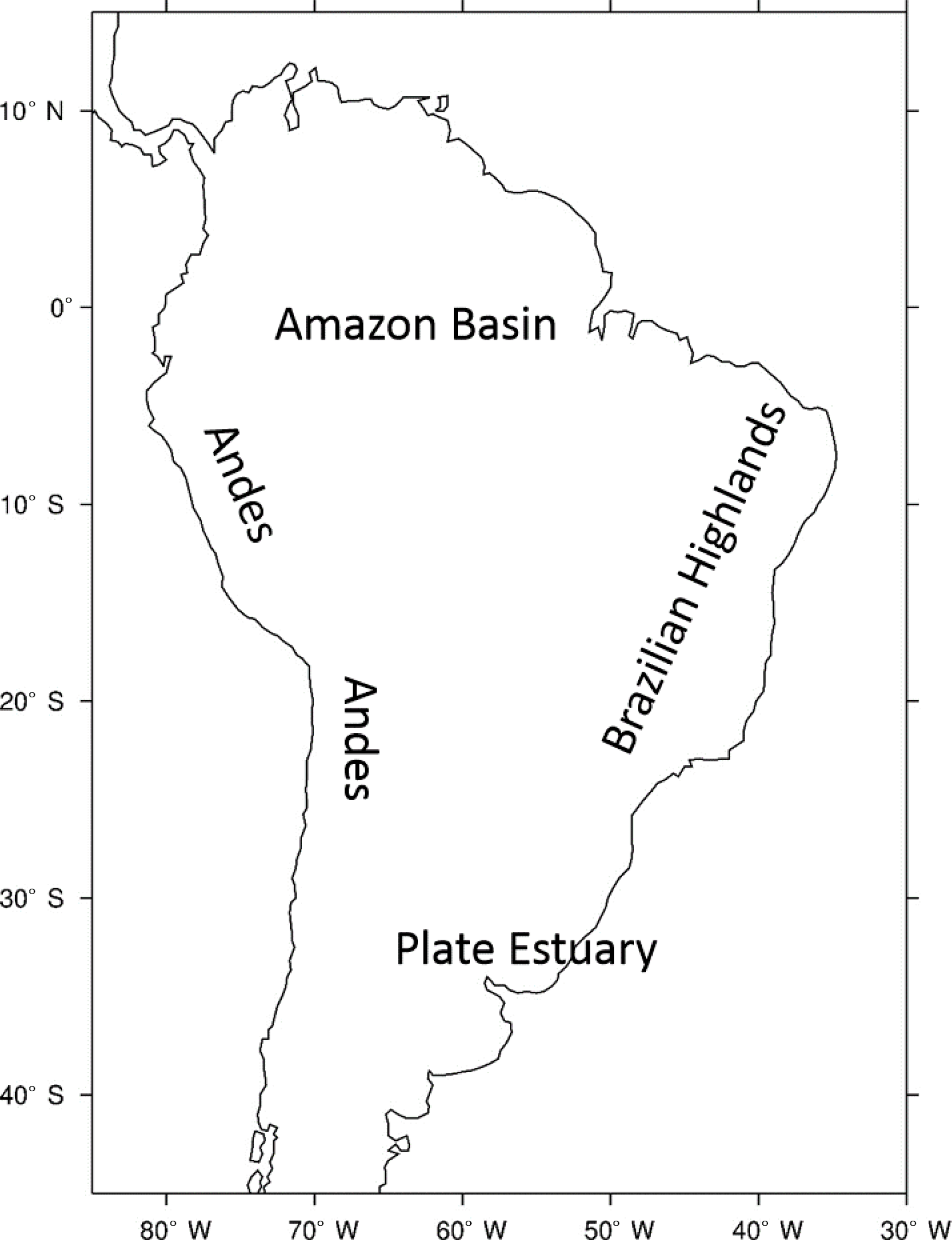
The climate of South America shows considerable variability, due to its large latitudinal extent (12∘ N to 53∘ S) covering tropical, subtropical and extratropical climate zones. The Andes also produce large east–west variation, compounded by the change in the east–west width of the continent and the differences between the temperatures of the oceans, with the south-western Atlantic being warm and the south-eastern Pacific being cool (Garreaud et al., 2009). In the tropics the intertropical convergence zone corresponds to an east–west belt of low pressure and low-level convergence of the trade winds, resulting in an area of high annual mean precipitation which is largely produced by deep convective clouds. The annual precipitation shows a seasonal cycle, with austral winter (JJA) maximum rainfall in the north of the continent. Towards the end of October the convection shifts southwards, so that the austral summer is characterized by heavy precipitation from the southern Amazon basin to northern Argentina. During the austral autumn (MAM) the maximum precipitation moves back to the north. This seasonal pattern is considered by some to be monsoonal (Vera et al., 2006; Marengo et al., 2012), although it does not exhibit the reversal in low-level winds seen in other monsoon systems. The South American monsoon generally has an onset in October, but the exact timing is variable, and geographically dependent, with an extension of the rainy area in the north-west of Amazonia down to southern Amazonia (Zhang et al., 2009). Generally there is an increase in precipitation from the north-west to the south-east from central America to the SE Amazon area, with the largest changes in the central Amazon area. Changes in the surface fluxes, with increases in surface radiation and sensible and latent heat flux, are considered to be initiators of the monsoon (Zhang et al., 2009). As the monsoon progresses, surface (sea level) pressure is expected to reduce over the South Atlantic, while the subtropical high in the South Atlantic is displaced eastwards and weakens (Marengo et al., 2012). Increased convection moves down from the north-west to central Amazonia and Brazil, while the circulation pattern at 850 hPa changes from northerlies to north-westerlies (Raia and Cavalcanti, 2008) in the south-west part of Amazonia, and in eastern Brazil from easterlies to north-easterlies following the displacement of the South Atlantic high. Close to the mouth of the Amazon the large-scale northerly anomalies and the reduction of the zonal component of the trade winds are expected as part of the transition to the monsoon (Marengo et al., 2001).
The South American Biomass Burning Analysis (SAMBBA) project was designed to use ground-based and aircraft observations of South American biomass burning aerosols to investigate their impact on climate. It involved a consortium of international institutions, led by the UK Met Office and the National Institute for Space Research (INPE) Brazil, in partnership with the University of São Paulo and seven universities in the UK (Exeter University, Leeds University, Manchester University, University of Reading, University of East Anglia, University of York, King's College London). The observational flights were conducted in September 2012 over the Amazonian region and were coordinated with ground measurements (Allan et al., 2014; Brito et al., 2014; Marenco et al., 2016). The flights were designed to measure aerosol properties, the atmospheric chemistry, and the clouds, meteorology and radiation budget over Amazonia. The modelling presented here is part of the complementary effort to use the flight campaign observation results to refine BBA properties in global models and to ascertain the effects of these aerosols on regional climate.
In this article we test the sensitivity of the (regional) South American climate to realistic high- and low-BBA-emission scenarios using aerosol properties constrained by aircraft campaign measurements. The main biomass burning months are August and September, so the results discussed in this paper focus on the changes in climate in September where the effects of the BBA on the regional climate are likely to be greatest, with a particular emphasis on cloud changes, the semi-direct effect and changes in atmospheric stability which impact cloud changes. Finally, we also briefly examine the influence of changing emissions of BBA on the South American monsoon onset. Section 2 describes the methodology and model set-up, Sect. 3 describes the results for the September biomass burning season, Sect. 4 focuses on the impact on the monsoon, and Sect. 5 discusses the results and their significance.
2.1 Model set-up
Global climate model simulations were performed with the Met Office Unified Model HadGEM3 GA3 (Hewitt et al., 2011) at the resolution of N96 (1.25∘ by 1.875∘) with 85 vertical levels. Simulations were run for 30 years, using annually repeating prescribed sea surface temperatures in order to minimize short-timescale variability and improve the statistical analysis. A spin-up period of 1 year was used. Sea surface temperatures and sea ice were prescribed using data from HadISST (Rayner et al., 2003) using monthly means over 1997–2011. Greenhouse and other trace gases are fixed at levels representative of 2000, identical to Shaffrey et al. (2009). Ozone is a seasonally varying two-dimensional latitude–height field from Randel and Wu (1999). The cloud scheme used was the PC2 scheme (Wilson et al., 2008a, b). Monthly emission periodic climatologies for non-BBA are used, including the 2-D sulfur cycle, black carbon and organic carbon from fossil fuel burning, from the CMIP5 dataset (Lamarque et al., 2010) with monthly means representing 2000–2010. Biogenic secondary organic aerosols are represented by an AOD climatology. The atmosphere was free-running.
Aerosols were simulated by the Coupled Large-scale Aerosol Scheme for Simulations in Climate Models (CLASSIC), a mass-based (“bulk”) aerosol scheme representing sulfate, fossil-fuel soot (black carbon), fossil-fuel organic carbon, biomass burning aerosol, sea salt and mineral dust aerosol species, where the physical and optical properties of each are specified and are externally mixed. A full description is given in the appendix of Bellouin et al. (2011), and Johnson et al. (2016) provide a detailed description of the BBA scheme.
The BBA scheme was originally introduced for HadGEM1 (Davison et al., 2004) and soon revised for HadGEM2 (Jones et al., 2005; Bellouin et al., 2007) to use updated BBA properties based on the SAFARI-2000 aircraft field observations from southern Africa (Haywood et al., 2003; Abel et al., 2003). In order to take advantage of these observations of ambient BBA available at the time, BBA was represented as a separate aerosol species, rather than as separate BC (black carbon) and OC (organic carbon) components. Mass is emitted into a fresh mode, and subsequently converted into an aged mode with an e-folding timescale of 6 h represented by an increase in mass by a factor of 1.62 (Abel et al., 2003). The fresh and aged BBA modes are represented separately in CLASSIC, with different optical, hygroscopic and CCN properties for each (see Sect. 2.3). The fresh and aged modes correspond to different OC : BC ratios, which is justified by the fact that BC and OC are internally mixed in BBA particles. The increase in BBA mass with ageing represents an increase in the mass of OC in BBA as the aerosol ages chemically and physically from condensation of VOCs within a plume. Although many GCMs now represent BBA as separate components comprising BC and OC, it is still advantageous to represent BBA as a single species with fresh and aged modes, since both aircraft and remote sensing observations characterize the ambient BBA rather than the BC and OC components. Therefore although climate models which separate BC and OC may appear more sophisticated, we lack the observational constraint to support and validate their complexity, particularly in BBA source regions. In this capacity, the BBA aerosol model properties and results can still be adjusted and/or validated using the more recent SAMBBA field campaign results, which for the most part also represent the ambient BBA rather than their BC and OC components.
Since the 6 h e-folding timescale is relatively short on a climate simulation timescale, most BBA in our simulations resides in the aged mode. Fresh BBA is not considered hydrophilic in CLASSIC. However, aged BBA exerts an indirect effect on clouds, acting as a cloud condensation nuclei (CCN), and is converted to smoke in cloud water by nucleation scavenging (analogous to sulfate aerosol in the model). Cloud droplet number concentration (CDNC) is calculated from the number concentration of CCN in the accumulation mode of BBA according to Jones et al. (1994, 2001) using a relationship based on multiple aircraft observations and assuming externally mixed aerosols. CDNC is used to calculate cloud droplet effective radius for the radiation scheme and for the autoconversion rate of cloud water to rainwater in the large-scale precipitation scheme (Bellouin et al., 2011). BBA is removed by wet and dry deposition. In the simulations here, we adjust the optical and hygroscopic growth properties based on observations (see Sect. 2.3) as we find BBA in the CLASSIC scheme demonstrates too much hygroscopic growth and not enough absorption (see Johnson et al., 2016, for more details).
2.2 BBA emission experiments
This paper compares the results of two 30-year climate simulations with high- and low-BBA emissions. Fresh BBA emissions are injected into the atmosphere as surface emissions (in the lowest model level), as well as at high levels (equally in mass across model level 3 to 20 – roughly equivalent to altitudes up to 3 km) in order to represent burning plumes reaching higher altitudes. No plume rise routines are incorporated and burning plumes are not explicitly represented in the model. Recent work found that simple plume height parametrizations are sufficient in representing BBA emission heights for global climate modelling (Veira et al., 2015), and the vertical parameterization of emissions is also justified by the fact that CLASSIC is able to adequately represent the vertical profile of BBA in terms of shape and total column AOD compared to observations (Johnson et al., 2016).
Monthly emission datasets are taken from Global Fire Emission Dataset (GFED) version 3.1 (van der Werf et al., 2010) for BC and OC. The emissions are summed to provide total BBA emissions in terms of carbon mass, allowing CLASSIC to incorporate oxygen mass and therefore calculate BBA mass. Emissions from GFED3.1 are provided in terms of vegetation sector: forest and deforestation fires provide high-level emissions, while savannah, woodland and peat provide surface emissions. This method does not allow for any spatial variation in BBA properties (such as optical properties) due to spatial variations in vegetation and/or burning type. However, additional simulations were run with varied BBA absorption properties, and results indicate that these changes were small, so we consider this impact to be minimal.
In all experiments the BBA emissions are scaled up by a factor of 2, in order to produce agreement between modelled and observed AODs, a measure that has been necessary in previous modelling studies using GFED3.1 (Reddington et al., 2015; Johnson et al., 2016, and references therein). Applying a global biomass burning emission scaling factor is an important assumption, but is not new to this study. Reddington et al. (2016) (their Table 2) show that multiple modelling studies have used scaling factors of up to a value of 6 in the past; attempting good agreement between modelled and observed BBA AODs and particulate matter concentrations is an ongoing problem. Johnson et al. (2016) also discuss the issue, noting that many studies have had to apply emission scaling factors greater than 1 in order to gain agreement between modelled and observed AODs and/or particulate matter measurements for BBA regions, such as Kaiser et al. (2012), Marlier et al. (2012), Petrenko et al. (2012), Tosca et al. (2013), Archer-Nicholls et al. (2016), Kolusu et al. (2015) and Reddington et al. (2016). Johnson et al. (2016) use a scaling factor of 1.6 for CLASSIC specifically, and here we increase this to 2, which is required to be higher as a consequence of decreasing the f(RH) curve to be consistent with the SAMBBA aircraft observations (see Sect. 2.3). Reddington et al. (2016) find that of many model aerosol properties, hygroscopic growth factors were the most important in determining the required emission scaling factor. Thus we might expect to need to increase modelled hygroscopic growth in order to match models and observations of BBA; yet we find the reverse: the SAMBBA observations suggest that CLASSIC is already too hygroscopic (Johnson et al., 2016 and this work, Sect. 2.3). It should also be noted that there are significant differences between different emission inventories, as well as between subsequent versions of the same emission dataset (van der Werf et al., 2010; Reddington et al., 2016), which may contribute to additional adjustments required in GCM emission schemes. We encourage further work in this area – both by future field work and modelling studies as well as for emission inventories – in order to reduce these important uncertainties.
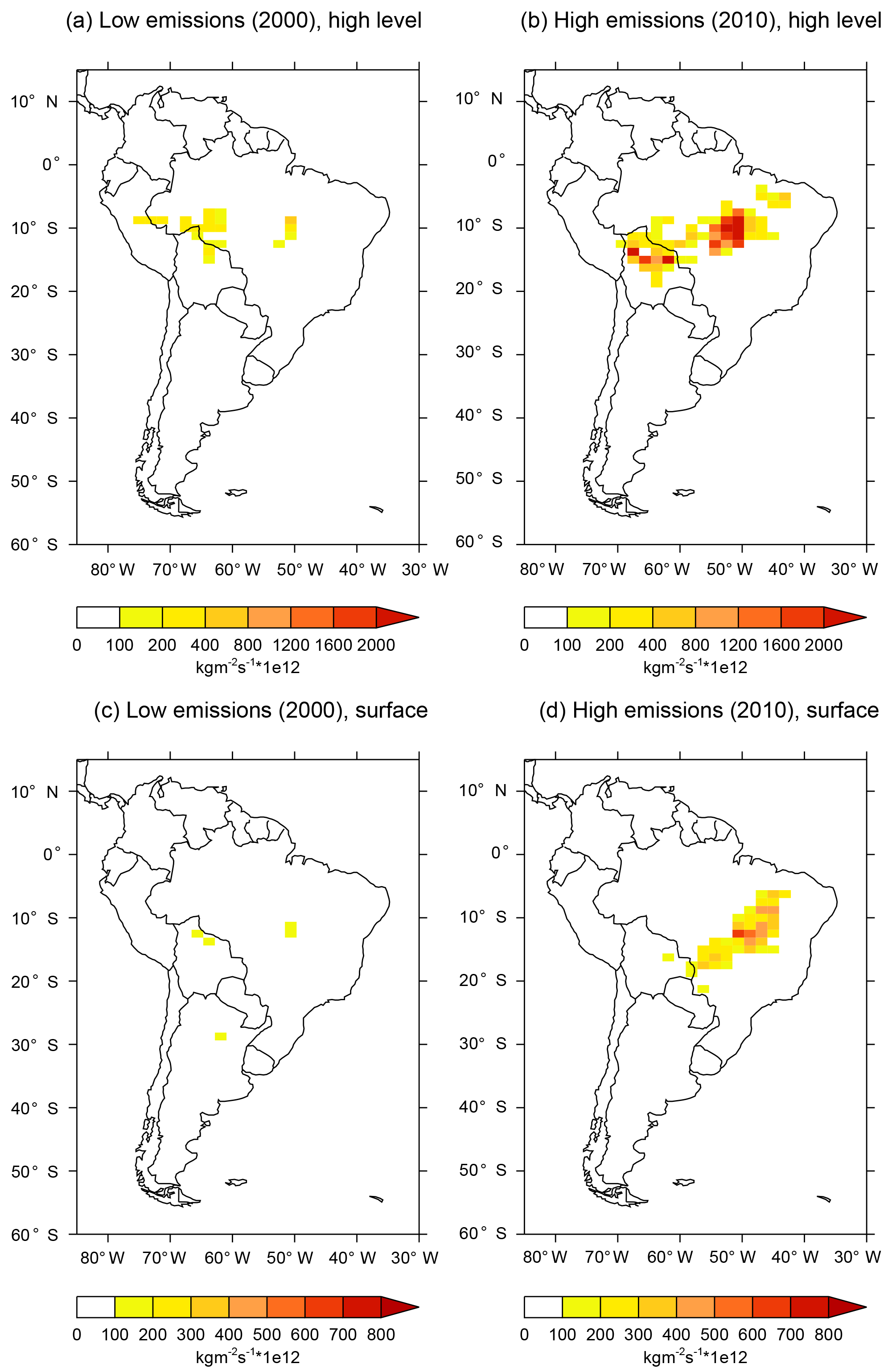
Figure 2BBA September fire emissions for the low (a, c, 2000) and high (b, d, 2010) emission experiments as applied in CLASSIC, from the GFED3.1 dataset. Panels (a) and (b) show high-level BBA emissions, (c) and (d) show surface emissions. Note the different scales between upper and lower panels.
In order to test the sensitivity of climate to the BBA loading within the South American region (60∘ S to 15∘ N and −85 to −30∘ W) we define two experiments to correspond to high and low emission cases, based on realistic variations of emissions observed for the South American region. During 1997 to 2011, the time period covered by GFED3.1 data, the highest emission year for the South American region was 2010, while the lowest emission year was 2000. Therefore high- and low-BBA-emission experiments are defined using South American BBA emissions from 2010 and 2000 respectively. Total annual emissions for the high and low emissions experiments for the South American regions are 0.51 and 2.32 Tg respectively (including both high-level and surface emissions). The geographical distribution of emissions for September 2000 and September 2010, the month of largest emissions, are shown in Fig. 2. Outside of South America, BBA emissions are set to the 1997–2011 GFED3.1 mean, with monthly variations, and do not vary between experiments, in order to place the focus of the experiment solely on the impact of changing South American emissions.
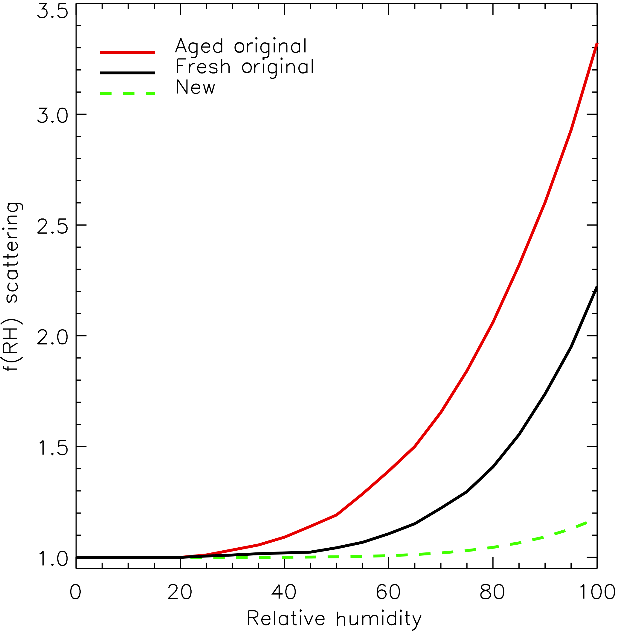
Figure 3The f(RH) scattering curves used in the CLASSIC aerosol scheme for BBA. Red and black lines show the standard hygroscopic scattering behaviour for fresh and aged BBA, and the green dashed line shows values applied in this work, taken from Kotchenruther and Hobbs (1998) for Porto Velho, Brazil.
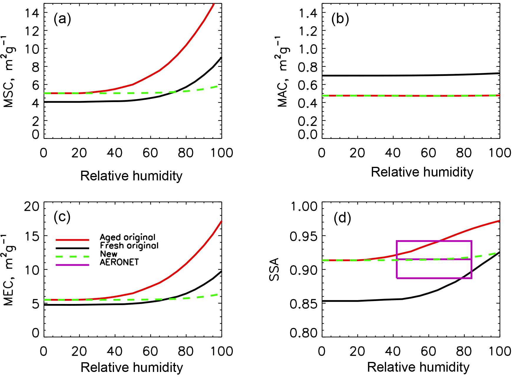
Figure 4Optical properties used in the standard CLASSIC configuration for BBA at visible wavelengths (black: fresh BBA; red: aged BBA) and the new representations applied in this work for fresh and aged BBA (green dashed line). (a) Mass scattering coefficient; (b) mass absorption coefficient; (c) mass extinction coefficient; (d) single scattering albedo. AERONET SSA at 550 nm is also shown (purple) with horizontal lines indicating long-term maximum, mean and minimum (see text for details).
2.3 Hygroscopic growth and optical properties in the modified CLASSIC scheme
This section describes how the hygroscopic growth and optical properties for BBA are altered from the standard CLASSIC values in order to be more in line with observations, including those from the recent SAMBBA intensive aircraft observations made during September 2012 (Johnson et al., 2016; Darbyshire et al., 2017).
Figure 3 shows the hygroscopic scattering growth curve (f(RH)) of BBA in CLASSIC, and Fig. 4 shows the dependence of scattering, absorption, extinction and SSA on relative humidity. Optical properties in CLASSIC are derived from aircraft measurements made during SAFARI-2000 of southern African BBA (Abel et al., 2003) and scattering hygroscopic growth is taken from Magi and Hobbs (2003) (MH2003), also for southern African BBA. CLASSIC allows for the separate representation of optical properties and hygroscopic growth of the fresh and aged BBA modes. The f(RH) values at 80 % RH are 1.5 and 2.2 for fresh and aged BBA respectively (see Fig. 4), demonstrating a very strong scattering increase at high humidities. Absorption in the model is not sensitive to RH (Fig. 4b), which is borne out by more recent measurements (e.g. Brem et al., 2012). Since extinction is the sum of scattering and absorption, extinction in CLASSIC is also strongly sensitive to RH, as is the single scattering albedo (SSA) (Fig. 4c and d).
However, CLASSIC is not consistent with other measurements. For example, Kotchenruther and Hobbs (1998) (KH98) performed aircraft measurements in the Amazon region around Brazilia, Cuiabá, Porto Velho and Marabá, and found much lower f(RH) values for BBA in the range of 1.05 to 1.29 at 80 % RH for regional haze from four different regions of Amazonia. Johnson et al. (2016) find that CLASSIC overestimates BBA hygroscopic growth, and therefore aerosol scattering, AOD and SSA in moist conditions. In this work, we apply the f(RH) curve of KH98 from Porto Velho, which was closest to the location of the SAMBBA observations, and represents the lower bound of the KH98 f(RH) curves (1.05 at 80 % RH), as a weakly hygroscopic case that gives a more reasonable representation (as indicated by the green dashed line in Fig. 3) than the existing CLASSIC properties. Since this f(RH) selection represents the lower bounds of f(RH) from KH98, the AODs from the model should be viewed as a lower limit, and could still be reasonably increased by selecting f(RH) values of up to 1.29 at 80 % RH.
It is not clear why the f(RH) curves of MH2003 for southern Africa and KH98 for Amazonia are so different, since both were observed with an airborne humidified nephelometer, and MH2003 do not comment on the differences. However, Johnson et al. (2016) hypothesize that the “regional air” classified in MH2003 may have contained a substantial amount of hygroscopic industrial sulfate aerosol, which could have behaved differently. Davison (2004) show some evidence that if combustion of peat swamps is involved, gas-to-particle conversion can produce high sulfate contributions in the BBA. We anticipate new state-of-the-art observations from the recent CLARIFY project observations within the southern African BBA plume to expand on this issue.
Figure 4 shows the new optical properties applied in this work. Scattering values are defined as identical to the original CLASSIC aged values at 0 % RH, but increase as a function of RH according to KH98 for the more realistic Porto Velho BBA observations. The RH dependence and absolute values of absorption are kept identical to the original CLASSIC data. Since extinction is the sum of absorption and scattering, extinction at 0 % RH is identical to the original CLASSIC data, but is much lower at high levels of moisture due to the lower f(RH) scattering dependency.
Additionally, although Fig. 4 shows a clear difference in optical properties in original CLASSIC between the fresh and aged BBA modes, the recent aircraft observations from SAMBBA did not reveal any differences between fresh and aged BBA, except possibly for very fresh BBA close to the source, under 1 h from emission (William Morgan, personal communication, 2015). Therefore in these experiments, since fresh BBA represents aerosol within 6 h of emission, we set the optical properties of fresh and aged BBA to be identical based on the new curves in Fig. 4.
As a result, the new SSA (Fig. 4d, green dashed line) is close to the standard CLASSIC SSA values for aged BBA at low RH, and close to the standard CLASSIC SSA values for fresh BBA at high RH. The new values are also in agreement with long-term inversion data from the AERosol Robotic NETwork (AERONET) stations (purple box) in the BB region, for six sites (L1.5 data from Ji_Parana SE, Rio_Branco, Alta_Floresta, Abracos_Hill, Balbina, Manaus_EMBRAPA) which have more than 1 year of data in the BB season (August–October). Horizontal lines shown in Fig. 4 represent maximum, mean and minimum SSA at 550 nm (linearly interpolated between 440 and 675 nm) across the 6 sites. The range of RH covered by the AERONET box represents typical values encountered during the SAMBBA aircraft research flights.
A wide range of SSA values for BBA is indicated from different observations, as discussed by Johnson et al. (2016). For example, SAMBBA aircraft observations show that cerrado burning in the eastern regions produces more BC and less organic aerosol, and therefore a more absorbing BBA at 550 nm (SSA = 0.79), while forest burning in the west produces less absorbing BBA (SSA = 0.88 ± 0.05) (Johnson et al., 2016; Hodgson et al., 2017). The range of AERONET retrievals shown in Fig. 4 is 0.89–0.94 (mean 0.92). Satellite-based retrievals of BBA indicate even higher SSA values (William Morgan, personal communication, 2015). Therefore since the various observations of SSA vary greatly, an intermediate value of SSA of 0.92 at 60 % RH seems reasonable for these experiments, as shown by the dashed line in Fig. 4d. Further experiments were run with varied absorption but are not presented here. Optical properties in all of the six spectral bands covering the visible wavelengths were adjusted using the same procedure.
3.1 Introduction
September has the highest biomass burning emissions which can directly influence surface fluxes whilst in situ, so we look first at September monthly-mean fields. For quantitative results we define a “biomass burning box” (BB box) (5–15∘ S, 40–70∘ W), selected on the basis that this is the main area where AOD is affected by biomass burning aerosol. The statistical significance for all plots is determined by a Student's t-test using the 30-year time series to identify where differences are due to the changes in the emissions, and not just inter-annual variability. We will examine the effects of the aerosol emissions on the AOD, and the consequences of the AOD changes on the clouds, the longwave (LW) and shortwave (SW) radiation and the surface fluxes, as well as the surface temperature, pressure, circulation and precipitation. The results are shown in Table 1, which gives the mean effect within the BB box on several variables for the high emissions case, low emissions case, and the difference (see Fig. 5a for the extent of the BB box).
Table 1Table of September mean values for the high and low experiments and the differences between them. The percentage changes in the table are calculated as (high − low) ∕ high. The means are calculated over the biomass burning box (latitude 5–25∘ S, longitude 40–70∘ W), which is outlined in Fig. 5a.
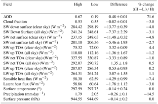
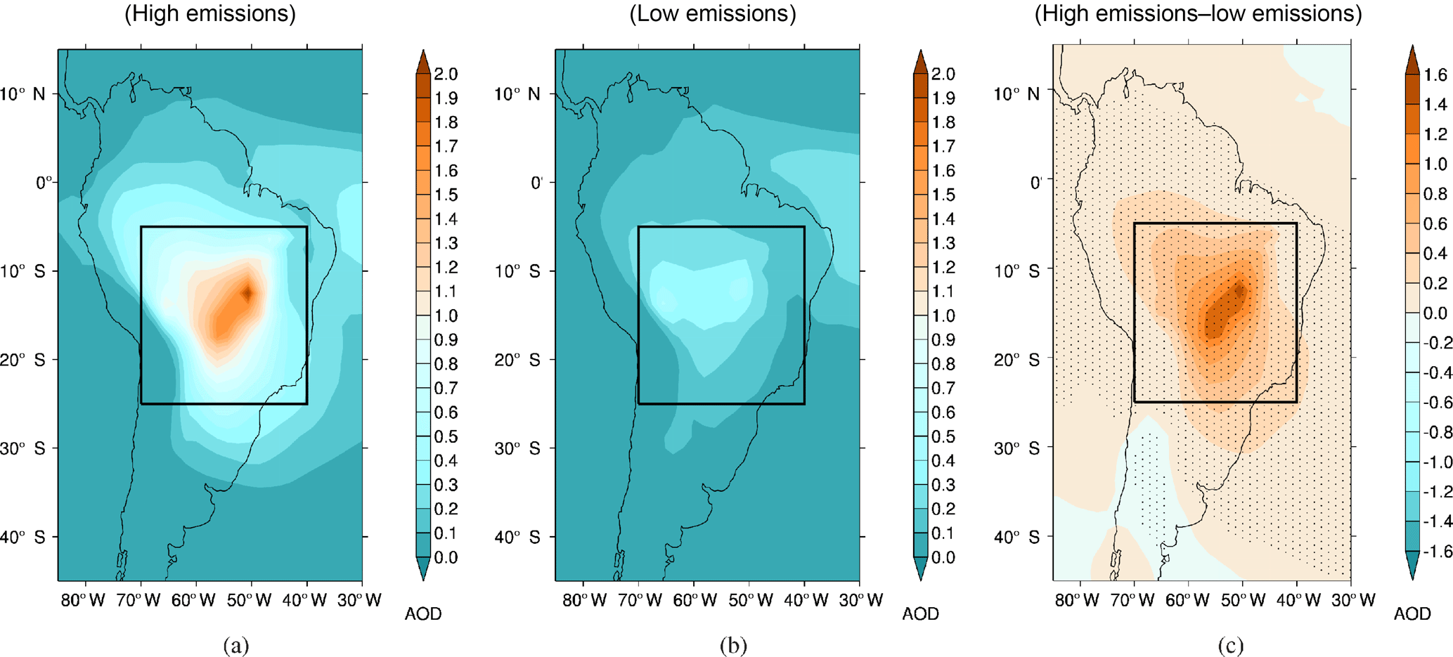
Figure 5(a) The September mean biomass burning AOD at 0.44 µm for the high emissions experiment. The outlined box contains the area used to calculate mean values in Table 1. (b) The September mean biomass burning AOD at 0.44 µm for the low emissions experiment. (c) Plot of the difference in the September AOD between the high and low emissions experiment. Stippling represents 95 % confidence limit.
3.2 AOD and clouds
Figure 5a and b show the biomass burning AOD at 0.44 µm over the 30-year HadGEM3-GA3 run for the high and low emissions case respectively. The high emissions case has a maximum BB AOD of approximately 1.6 across the central biomass burning area, and values of up to 0.3 extend to the north and south. The mean value for the outlined box is 0.68 ± 0.01. In the low emissions case the highest values are 0.6, with lower values of 0.1 over most of the biomass burning area; the mean in the box is 0.19 ± 0.005 (see Table 1). In both cases African biomass burning results in a small transported BB AOD across the South Atlantic, which extends to the coast of South America. In the two model runs, the biomass emissions from Africa (and the rest of the world) are identical and are based on climatological means. The differences (high − low) in BB AOD between the two runs (Fig. 5c) are greatest over the BB region, as expected; the BB AOD transported from Africa shows no difference between the two runs, confirming that this is not the result of South American BBA. The mean BB AOD difference in the BB box area is 0.48, a reduction of 71.6 % from the high case to the low case. As discussed in the previous section, the difference in emissions is 78 %, suggesting that the majority of the emissions change is translated to a BB AOD change. The direct relationship between particulate emission from fire and observed AOD in South America is noted by Reddington et al. (2015).

Figure 6(a) The September mean cloud fraction for the high emissions experiment. (b) The September mean cloud fraction for the low emissions experiment. (c) Plot of the September difference in the cloud fraction between the high and low emissions experiment. Stippling represents 95 % confidence limit.
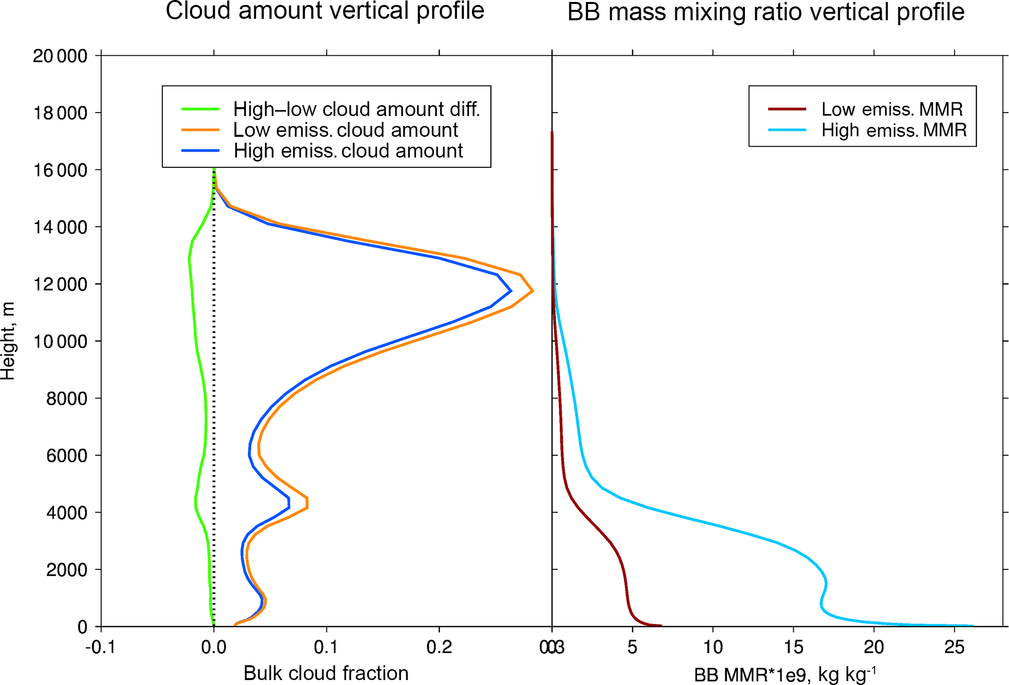
Figure 7September mean vertical profile of cloud fraction for high emissions, low emissions, H − L compared with the vertical profile of the aerosol burden mass mixing ratio (MMR) in kilograms per kilogram (kg kg−1) (both quantities averaged over BB box area outlined in area plots).
In Fig. 6a and b the total September average cloud fraction for the high and low emissions experiments are plotted, showing the distribution of cloud cover. In both cases the highest cloud fractions are over the far north-west part of the continent, down into the Amazon basin. Along the east coast and into the Brazilian Highlands (centred on 15∘ S, 45∘ W) there is less cloud cover, although it increases again towards the Plate estuary (35∘ S, 58∘ W). There is also little cloud over the Andes, but a substantial fraction over the eastern edge of the Andes mountain range, and high cloud over the Caribbean area (12∘ N, 47∘ W). In Fig. 6c the change in cloud fraction between the high and low emissions case is plotted – the stippled areas denote a confidence level of 95 %. The cloud fraction is reduced by 0.05 in much of the biomass burning area (3.8 % averaged over the BB box), although there is a substantial effect to the north-east of the main AOD difference (Fig. 5). The reduction in cloud would be consistent with semi-direct effects found in other modelling studies, whereby increased atmospheric heating can reduce convective activity and burn off the clouds within the aerosol layer (Koch and Del Genio, 2010). Outside of the area with high AOD differences higher emissions appear to result in a slight increase in cloud fraction in the area to the east of the Andes and just north of the River Plate valley (34∘ S, 55∘ W); however, the changes in these areas are not statistically significant at the 95 % confidence level.
The profile of cloud fraction with height (averaged over the area outlined in Fig. 6a) is shown in Fig. 7 for the high and low emissions cases. The biomass burning burden profiles are shown for comparison. Cloud layers are evident at about 1 and 4.2 km, and the presumed outflow from deep convective clouds at 9–14 km. Despite September being the dry season these clouds were frequently observed from the aircraft during the SAMBBA aircraft campaign (Marenco et al., 2016).
In general the low emissions case has more cloud at all levels, with the most marked differences in the high cloud amount at 9–14 km, and the mid-level cloud at 3–6 km. Cloud changes below 2 km are small, in part because cloud cover at these heights is minimal. Koren et al. (2004) suggest a reduction in boundary-level clouds can occur where aerosols stabilize the boundary layer and cool the surface, since the supply of water from the forest canopy is reduced. Where the aerosol and cloud are at the same height, i.e. below around 4 km, we would expect the reduction via the semi-direct effect to be strongest as the heating of the atmosphere due to the presence of absorbing aerosol promotes cloud evaporation (Koch and Del Genio, 2010). However, we see a similar magnitude of cloud reduction for the medium-level (3–5 km) and the high clouds at 9–14 km, where the aerosol burden is much lower. A likely mechanism for this reduction in medium and high cloud cover would be the stabilizing of the atmosphere, due to the aerosols in the lower levels heating the atmosphere but cooling the ground, stabilizing the boundary layer, reducing its height and thus reducing the amount of deep convection occurring in the high emissions case (Koren et al., 2008). In Fig. 8a the stable boundary layer diagnostic (which is defined to be set to 1 where the surface buoyancy flux is < 0.0, at each time step and each grid point; the average indicates the fraction of time in this state) shows that the high emissions case has a more stable boundary layer, especially in the areas where we see the most cloud reduction. This tends to support the explanation that cloud reduction is related to the boundary layer changes. The boundary layer height varies between 1 and 1.8 km in the BB box, and in Fig. 8b the boundary layer height differences show a reduction for the higher BBA case, due to the reduction in SW radiation reaching the surface, and the reduction in sensible heat flux (Zou et al., 2017; Ackerman et al., 2000). The deep convection model diagnostic (defined to be set to 1.0 if deep convection occurs during a model timestep, 0 if not, similar to the boundary layer stability diagnostic mentioned above), shown in Fig. 8c, also shows the statistically significant reduction in deep convection for the higher emissions case, across most of the main area of BBA, and also the area to the west side of the Amazon Basin. There is a dipole change in the Caribbean, where the area along the north-east coast of South America shows a statistically significant reduction, and just to the north there is a (statistically significant) increase for the high emissions case. Although this is not entirely congruent with the area of highest AOD difference, it is clear that there is a significant influence of BBA on the deep convection as represented by this diagnostic, suggesting that the reduction in cloud fraction may be due predominantly to this mechanism. This change in deep convection between simulations is likely to be contributing to the high- and mid-level cloud changes, as in the model some of the mid-level cloud is likely due to detrainment of deep convective cloud around the freezing level.
Where evaporation is reduced and moisture availability for cloud formation is curtailed, this would also act to inhibit cloud formation (Koren et al., 2008); the relative humidity (not shown) in the high emissions case is higher at the surface (< 1 km) by around 10 %, but lower throughout the rest of the profile, with the largest difference (−7.5 %) occurring at around 5 km. With a more stable boundary layer in the high emissions case there is less turbulent transport of moisture from the surface layer. This would suggest a drier atmosphere at height is also contributing to reduced cloud formation in the high emissions case.
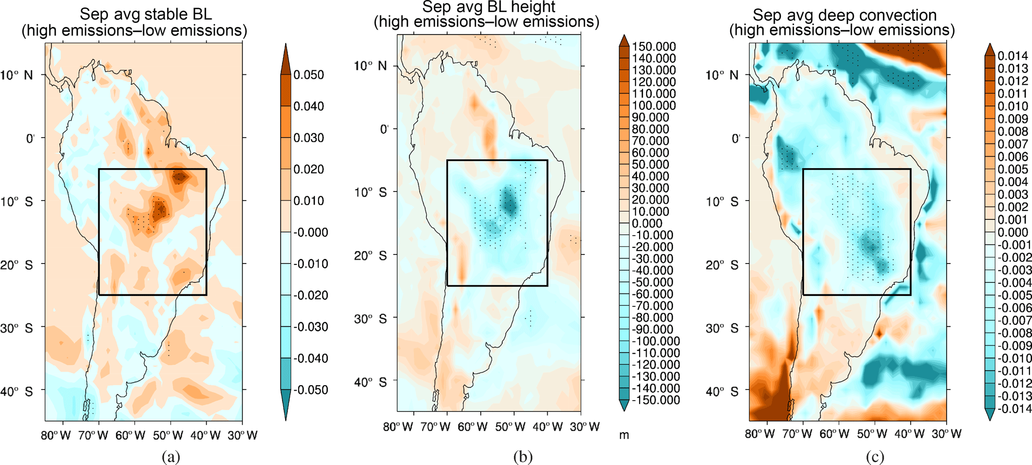
Figure 8(a) Plot of the September difference in the boundary layer stability diagnostic between the high and low emissions experiment. (b) Plot of the September difference in the boundary layer height between the high and low emissions experiment (m). (c) Plot of the September difference in the deep convection diagnostic between the high and low emissions experiment. Stippling represents 95 % confidence limit.
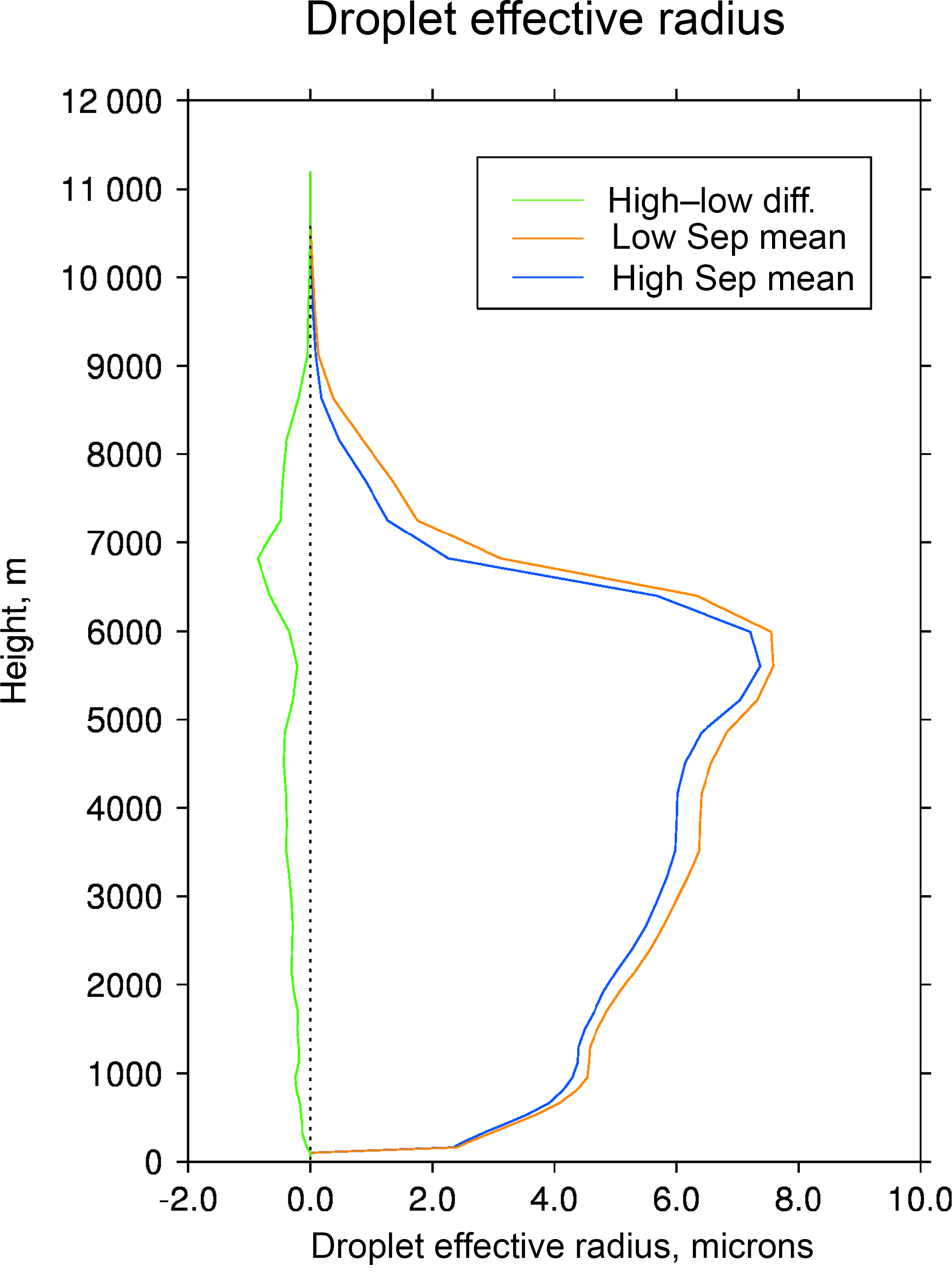
Figure 9Vertical profile of September mean differences of droplet effective radius (microns) (averaged over the BB box 5–25∘ S, 40–70∘ W)
Considering the indirect effect, in Fig. 9 we see a reduction in the effective radius of the liquid water drops where increasing the aerosol amount reduces the effective radius, as suggested by, for example, Warner (1968); Twomey (1977); Jiang and Feingold (2006); Rosenfeld (2000). The vertically integrated droplet concentration also increases for the higher emissions case, which is consistent with predictions that the increase in nucleation centres (aerosol particles) will increase the number of droplets. Ten Hoeve et al. (2012) and Wu et al. (2011) suggest that there is a competition between the microphysical effects and radiative effects, where high AOD results in reduced cloud where the radiative effects are dominant, which is consistent with our results.
3.3 Effects on radiation
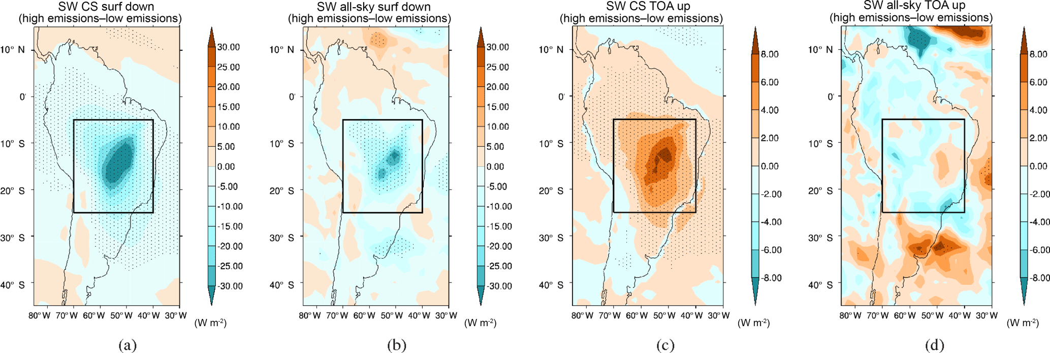
Figure 10The September mean difference between high and low emissions cases for (a) the clear-sky downwelling SW radiation at the surface, (b) the all-sky downwelling SW radiation at the surface, (c) the clear-sky upwelling SW radiation at TOA and (d) the all-sky upwelling SW radiation at TOA. Stippling represents 95 % confidence limit.
In Fig. 10a and b we see the difference between the high and low emissions case in the downward SW radiation at the surface, which largely follows the areal extent of the difference in the AOD. The results for the clear-sky (i.e. excluding all clouds) SW reaching the surface (in the BB box) from our models show the mean reduction in the September mean downwelling flux is −13.77 ± 0.39 W m−2 (a reduction of 4.8 %) for the high emissions case compared to the low emissions case. The all-sky differences include the effect of clouds and indeed changes in the cloud fraction reduce the area mean change to −7.44 ± 2.29 W m−2, indicating that scattering by the clouds above the aerosol reduces the difference we see due to the aerosol changes alone. The competing effects of the reduction in SW radiation at the surface due to the BBA and the increase due to reducing cloud cover control the resulting impact on the SW radiation at the surface, and in most of the BB box area the BBA has the stronger effect. There is also a statistically significant (at the 95 % confidence level) surface reduction in SW to the north of the Plate Estuary (34∘ S, 55∘ W), which we interpret as the effect of the increase in cloud in this area, as the BB AOD difference is very small here, while the cloud fraction increases (see Fig. 6a), resulting in the reduction of SW radiation at the surface here.
The top-of-the-atmosphere (TOA) upwelling SW radiation differences are shown in Fig. 10c and d, where the clear-sky differences show an increase for the high emissions case in the same area as the BB AOD differences between the two experiments. This illustrates the direct radiative effect, which is stronger with higher emissions. The all-sky case is much less clear-cut, as the influence of the clouds results in a predominantly negative difference. This suggests that the effect of the reduced cloud cover, and thus reduced scattering by clouds in the high emissions case, dominates over the increased scattering from the increased BBA (as seen in the clear-sky case). This changes the sign of the SW radiative effect at the TOA, causing a net reduction in outgoing SW in the region. These changes are not statistically significant, however.

Figure 11September mean differences: (a) The difference between high and low emissions case for the clear-sky outgoing LW radiation at TOA. (b) The difference between high and low emissions case for the all-sky outgoing LW radiation at TOA (note the colour scales for clear sky and all sky are different). (c) The difference between high and low emissions case for the column integrated water vapour.
The difference in outgoing longwave radiation at the TOA is shown in Fig. 11, where the clear-sky difference shows a generally positive change, such that the increase in aerosol results in an overall increase in the outgoing LW radiation over much of the biomass burning area. However, since the aerosol properties prescribed in the model relate to relatively small aerosol size the BBA has little effect on LW radiation directly. As the only significant changes are seen in areas outside the main biomass burning areas, it is much more likely that these LW changes are related to secondary effects, for example water vapour changes. Shown in Fig. 11c, the LW radiation changes are consistent with decreased column water vapour in the high emissions experiment, which leads to increased outgoing LW radiation at the TOA. The aerosol properties prescribed in the model relate to relatively small aerosol size, and therefore the effect of BBA on LW radiation is negligible. In the all-sky case (Fig. 11b), the differences are significant in the main biomass burning area, but can be directly related to the changes in cloud fraction between the high and low emissions case; where the clouds are reduced, we see a greater LW upwelling at the TOA, as the effective emitting temperature is now lower in the atmosphere and warmer.
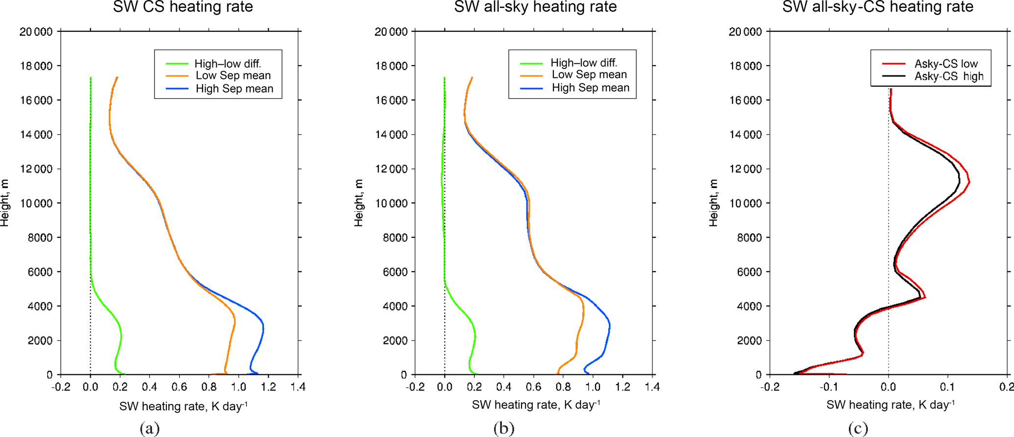
Figure 12September mean SW heating rates (averaged over the BB box 5–25∘ S, 40–70∘ W) for high and low emissions: (a) clear sky, (b) all-sky and (c) all-sky–clear-sky differences, showing heating rate changes due to cloud only.
The clear-sky SW heating rate is shown in Fig. 12a for the high and low emissions results. The largest difference between the high and low emissions case is below 5 km, coincident with the majority of the absorbing aerosol, resulting in an increased heating rate of the atmosphere for the high emissions compared to the low emissions case. As the BBA is absorbing (with an SSA < 1.0) it absorbs some fraction of the SW, and an increase in BBA results in an increase in the heating rate. The maximum heating rate also appears to be at a slightly lower altitude for the high emissions case. Above 5 km there is a much smaller difference, with a very slight negative difference at 9 to 15 km (i.e. the high emissions have a slightly lower heating rate at this altitude).
The all-sky heating (Fig. 12b) rate shows broadly similar characteristics, but we see a dip in the heating rate in both cases at 500 m height, which is more marked in the high emissions case, and subsequently there is a less linear profile in both high and low emissions cases. The presence of clouds provides absorption and scattering of SW radiation above the main BBA layer resulting in an increase in the heating rate at levels containing clouds, relative to the clear-sky case. The SW heating rate is reduced below the cloud, as less SW radiation reaches these altitudes and thus the heating rates here are reduced. The effect of the clouds is stronger in the low emissions case, as there is more cloud here, but the differences due to cloud cover compared to the clear sky are not large. The differences between the all-sky and clear-sky heating rates (Fig. 12c) illustrate the heating rate changes due to cloud only; beneath 4 km, clouds cause a cooling but differences between the two experiments are minimal. Above 4 km the clouds warm the atmosphere, with the extra cloud cover in the low emissions case producing a larger cloud heating rate than for the high emissions (reduced cloud) case.
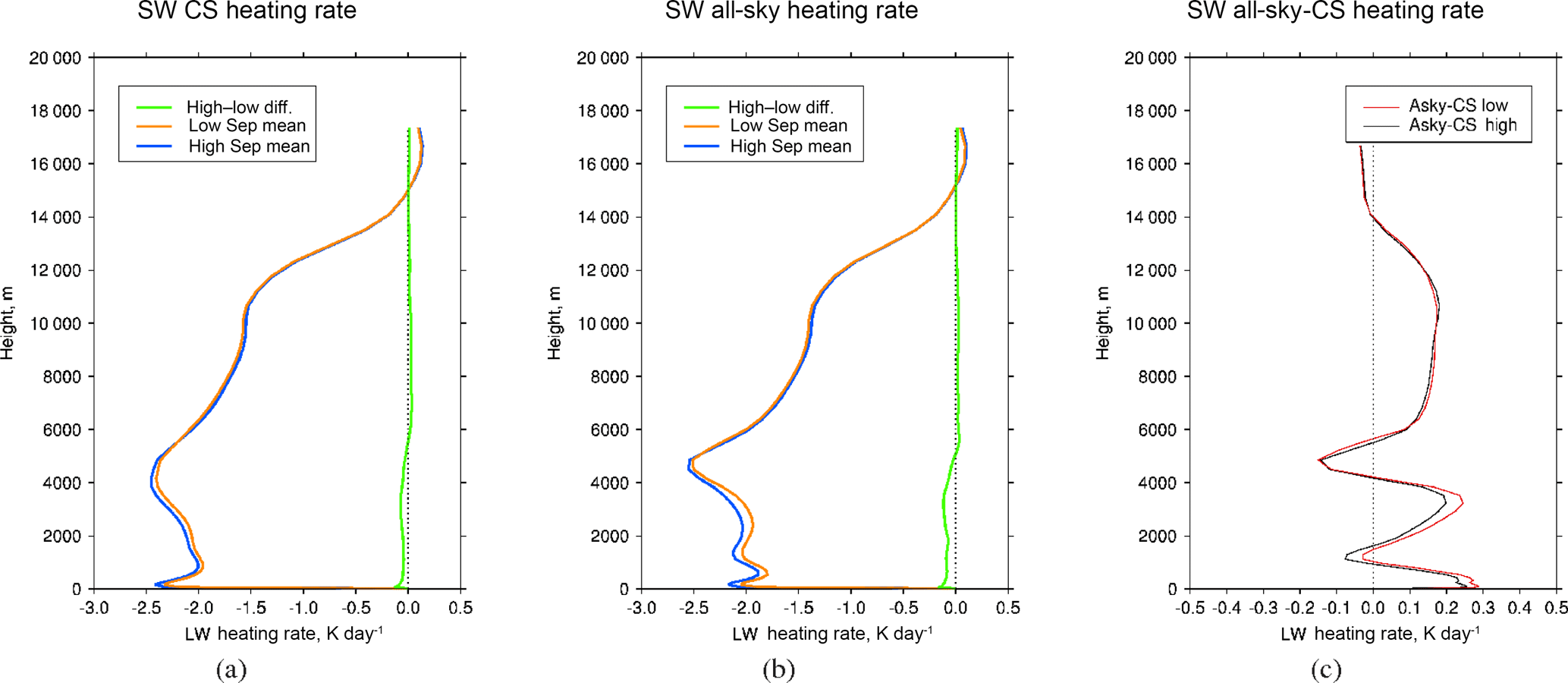
Figure 13September mean LW heating rates (averaged over the BB box 5–25∘ S, 40–70∘ W) for high and low emissions for (a) clear sky, (b) all sky and (c) all-sky–clear-sky differences.
In Fig. 13a the clear-sky LW heating rates show cooling up to 15 km (tropopause), with the largest cooling of −2.5 K day−1 at 4–5 km (note the difference in scales from the SW plots). The low emission experiments show less cooling than the high emission experiment below 6 km, which then reverses from 6 to 14 km. In the all-sky plot (Fig. 13b) we see below 4 km that a reduction in cloud leads to more LW cooling of the lower atmosphere. Above 4 km, the reduced cloud leads to a slight warming of the atmosphere due to the upward longwave emissions from below. Higher BBA emissions reduce the cloud cover resulting in a reduction in the absorption of radiation, and thus less LW re-emission from the clouds. There may also be an increase in LW emission due to the increased temperatures in the BBA layer (0–4 km). The all-sky–clear-sky difference plot (Fig. 13c) shows the impact of the cloud changes alone on the heating rates, demonstrating the effect of higher emissions reducing the cloud cover, reduced heating between the cloud layers (e.g. near the surface and at 3 km) and increased cooling within the cloud layers (1 and 4 km), but there is very little change at higher altitudes. Within the BBA layer we can see the semi-direct effect of the cloud burn-off, but the higher cloud (12 km and above) appears to be responding to stability changes.

Figure 14(a) September mean differences (high − low) for (a) sensible heat flux (b) latent heat flux. Stippling represents the 95 % confidence interval.
The effects of the BBA on the sensible heat flux are shown in Fig. 14a, where the higher emissions result in a reduced sensible heat flux, due to the reduction in SW radiation cooling the surface (cf. Fig. 10b). There are also significant differences around the Plate Estuary, which may be due to an increase in cloud cover in this area for the high emissions case which reduces the SW radiation reaching the surface, and thus also reduces the sensible heat flux. The spatial agreement with the main differences in BB AOD (see Fig. 5) is generally good, suggesting this is largely an effect of the increased BB AOD in this case. The latent heat flux differences show statistically significant reductions for the high emissions case in the area to the north of, and in the centre of, the main BB area. However, these changes are not strongly co-located with the BB AOD changes and are possibly related to reductions in available moisture due to reduced precipitation and circulation changes affecting the latent heat flux, which are investigated in the next section. These results are consistent with those of Zhang et al. (2008).
3.4 Meteorology

Figure 15September mean differences (high − low) for (a) surface temperature, (b) total precipitation (stippling represents the 95 % confidence interval) and (c) moisture flux differences at 850 mb; coloured contours are the magnitude of the moisture flux.
There is a mean change (in the BB box) in the surface temperature between the high and low emissions runs of 0.14 ± 0.23 ∘C, with a statistically significant maximum decrease of approximately 0.8 ∘C in the north part of the BB box. There is a maximum increase of approximately 0.5 ∘C around the southern part of the Brazilian highlands; however, this increase is not statistically significant (25∘ S, 50∘ W), as shown in Fig. 15a. The spatial pattern here reflects the BB AOD differences in part, where the absorption and scattering of SW by the aerosol reduces the surface temperature. There are increases in surface temperature where the clouds are reduced near the southern Brazilian Highlands; here the cloud reduction allows more of the SW radiation through, and the extinction due to the BBA is somewhat lower than in the north of the box. The competing effects of the direct effect reducing the SW radiation reaching the surface and the reduction in cloud cover increasing the SW radiation at the surface are clear, controlling the mixed geographical response of the surface temperature overall.
The differences in total precipitation are shown in Fig. 15b, where the overall effect in much of the northern part of the continent is a reduction in the total precipitation, particularly marked in the western Amazon basin and the Caribbean. Further south we see an increase in the area just north of the River Plate (30∘ S, 55∘ W), which corresponds to the area of increase in cloud fraction seen in Fig. 6; however, this increase is not statistically significant at the 95 % confidence level. The decreased aerosol in the low emissions case leads to a 14.5 % increase in precipitation in the BB box with mean precipitation increasing from 1.78 mm day−1 (high emissions) to 2.05 mm day−1 (low emissions).
The decrease in precipitation seen in the high emissions experiment is consistent with the reduced cloud and latent heat flux, and the more stable boundary layer seen in this experiment. The resulting reduction in precipitation could result in a reduction in soil moisture content, partly explaining the reduction in latent heat flux shown in Fig. 14b. Gonçalves et al. (2015) analysed rainfall data in the Amazon and suggest that the influence of biomass burning on precipitation is dependent in part on the degree of atmospheric instability. In a more stable atmosphere, BBA tends to decrease the precipitation; they also note that increasing cloud droplet number, and decreasing droplet size, would act to reduce precipitation in the absence of strong convection. In Fig. 15c the moisture flux at 850 mb shows the increase in moisture transported by the low-level jet east of the Andes, which together with the increased flux from the South Atlantic combines to produce the increase in precipitation seen at 30∘ S, 50∘ W.
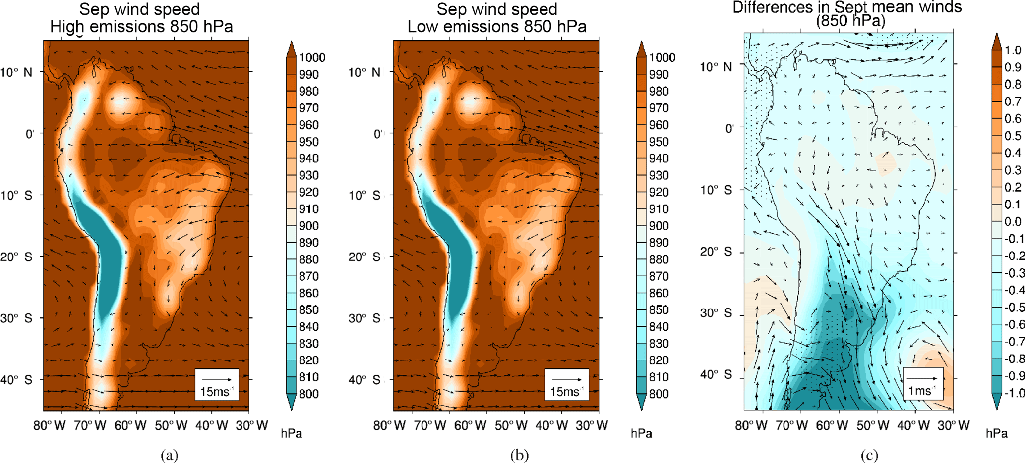
Figure 16September mean wind circulation at 850 hPa for (a) high emissions case (coloured contours are mean September pressure in hPa), (b) low emissions case, and (c) differences in pressure and wind circulation for high − low runs. Coloured contours in (a) and (b) are surface pressure and in (c) surface pressure differences in hPa.
The surface pressure and 850 hPa circulation for high and low emissions are shown in Fig. 16a and b. The ERA-Interim mean September surface pressure and circulation (averaged over a similar timescale) are shown in the Supplement (Fig. S1 and Fig. S2 in the Supplement) for comparison and show that in general both surface pressure and the circulation are well represented by the model, although the wind flow seems to be somewhat more zonal between 0 and 10∘ S in the ERA-Interim plot. The model results for surface pressure are broadly similar for both the high and low emissions experiments, with a high-pressure area in the central Amazon basin, and low pressure to the north and west. We also see high pressure along the eastern side of the Andes, down towards the River Plate estuary, and a high-pressure system in the south-east Atlantic, which shows some difference in position between the high and low emissions case. The surface pressure differences (Fig. 16c) show a slight increase in the Amazon basin area, but a larger decrease down in the southern part of Brazil and around the Plate Estuary. We also see a difference in the South Atlantic, which is related to the position of the South Atlantic high shifting between the high and low emissions case. The pressure differences are of the order of 1 hPa, with significant changes at the 95 % confidence level in the Caribbean area and in southern Argentina.
The change in pressure patterns corresponds to the change in winds at 850 hPa. (Fig. 16a and b). The general circulation is easterly across the Amazon basin, south-easterly in the Caribbean, and tending to north-easterly to the south of the Amazon mouth. In the southern part of Brazil we see a northerly direction, turning westerly at the southern tip of the continent. Although the overall circulation patterns are similar for the two experiments, we do see differences between the high and low emissions case in Fig. 16c, the largest effect being a strengthening of the low-level jet that runs along the eastern side of the Andes, from around 10 to 30∘ S, down to the Plate Estuary. Analysing the zonal and meridional components suggests that the most significant change is in the zonal component, possibly suggesting a change in direction as well as in strength. There is also a change in the circulation due to the shift in the South Atlantic high-pressure system, where the easterlies are weaker in the low emissions case, and have a more southward component in the high emissions case. In the Caribbean area the prevailing easterlies and south-easterlies are weaker in the high emissions case.
Fu et al. (1999) suggest that local thermodynamical processes may be important for onset of the monsoon, whilst the strength of the low-level jet to the east of the Andes is an important source of moisture for the subtropical convection that brings rainfall to the south of the region in the wet season (e.g. Liebmann and Mechoso, 2011). As these features appear sensitive to the aerosol emissions during September (see Sect. 3.4) we now consider whether there is any discernible difference in the transition to monsoon regime between high and low aerosol simulations. We do this in only a broad sense, since the temporal resolution of our output is not sufficient to identify a specific monsoon onset date, and in any case, the definition of onset is a matter of some debate in the literature (Liebmann and Mechoso, 2011). The transition to the wet season between September and November is broadly similar in the model as shown in previous studies (Raia and Cavalcanti, 2008; Liebmann and Mechoso, 2011; Marengo et al., 2001, 2012) and is comprised of the following
-
a shift to northerly and north-easterly wind across the Amazon basin,
-
strengthening of the northerly low-level jet to the east of the Andes,
-
eastward movement and weakening of the high-pressure system,
-
a shift to cross-equatorial rather than zonal flow to the north of the region,
-
increased rainfall over the Amazonian basin that extends southwards and eastwards moving through October and November.
These changes are shown in Fig. S5, where the high emissions case is used to show the mean November meteorology, exemplifying the changes described above.
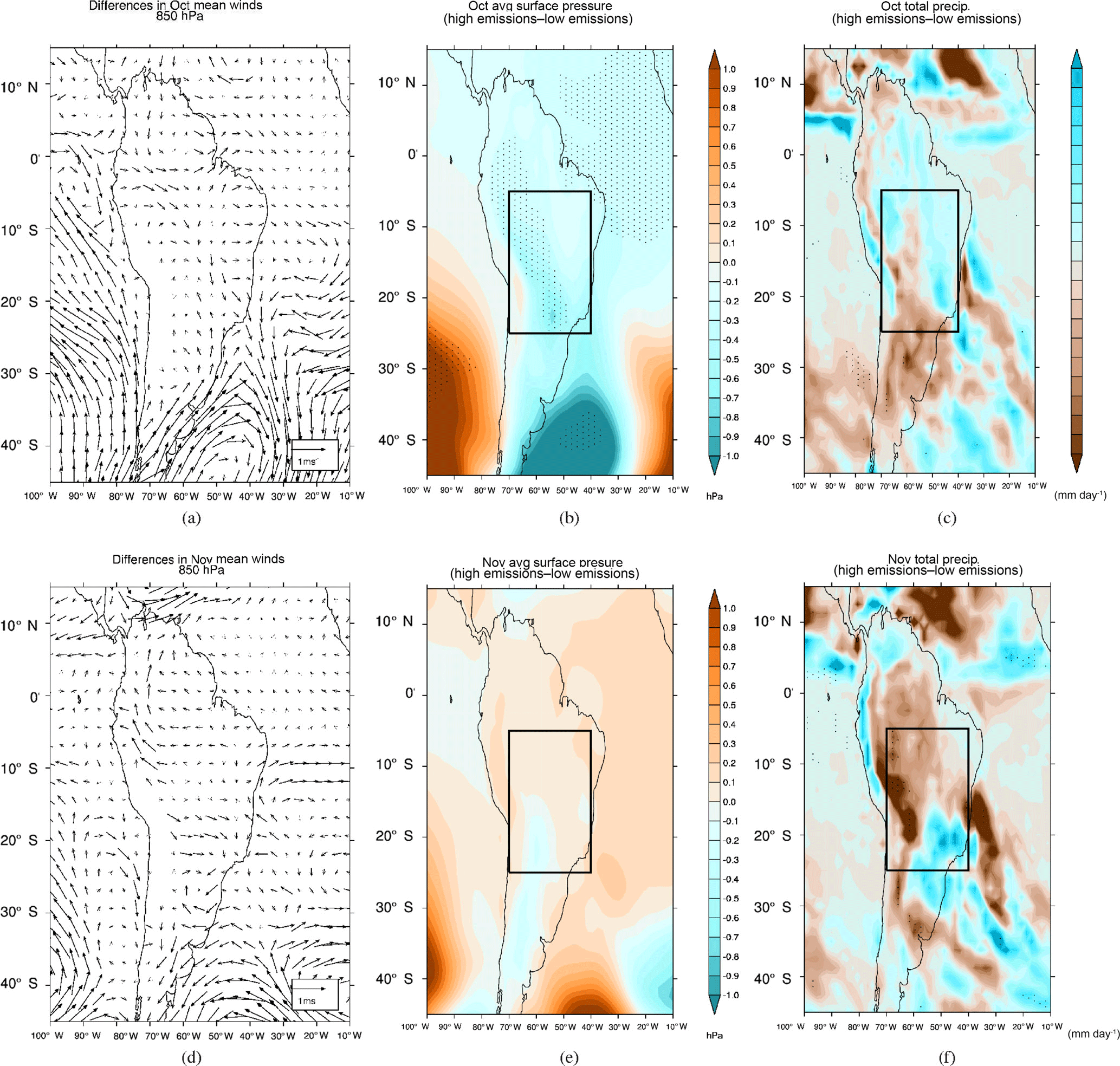
Figure 17Plot showing the differences in meteorological variables for October and November: (a) differences in mean circulation for October; (b) differences in mean surface pressure for October; (c) differences in mean precipitation for October; (d) differences in mean circulation for November; (e) differences in mean surface pressure for November; (f) differences in mean precipitation for November. (Note the difference in projection and area from previous plots.)
Significant differences are seen in October surface pressure between high and low emissions simulations across the South Atlantic and South Pacific, reflecting slightly different positions of the high pressure in each case, and on the east of the Andes where pressure is lower in the higher emissions case, but this does not extend into November (Fig. 17b and e). We do, however, find a significant decrease in November precipitation (Fig. 17f) across the Amazon basin area in the higher emissions simulations, which is consistent with enhanced transport of moisture from the Amazonian basin by the strengthened jet (Fig. 16c) on the east of the Andes in the high emissions case. The Freitas et al. (2005) examination of biomass burning in regional climate models suggested that aerosols might oppose the transition to monsoon state, with strong absorption stabilizing the troposphere in the southern Amazonian region. Whilst the results in our model suggest that the strengthening of the jet east of the Andes may also have an effect, further simulations with higher temporal resolution of output would be needed to establish the mechanism by which aerosol emissions appear to affect the monsoon rainfall.
The aim of the work described here was to investigate the impact of biomass burning emissions on the regional climate in South America using the Met Office Unified Model HadGEM3 GA3 model. We examine this through two 30-year climate runs with BBA emissions taken from the GFED v3.1 dataset, representing low and high emission years. We adjust ambient BBA optical and hygroscopic properties based on the literature and on recent airborne in situ measurements from the SAMBBA project. We employ a global BBA emission scaling factor of 2 in order to generate AODs comparable to observations. Reconciling surface particulate matter concentrations and AODs for BBA between models and observations is a continuing problem for climate models and the scientific community, largely impacted by the hygroscopic activity of BBA and choice of emission dataset and version, and we urge further research in this area in order to reduce modelling and observational uncertainties.
We have found clear semi-direct effects of the biomass burning aerosol in September, with the results indicating a significant burning off and an additional effect on cloud cover from reduced deep convection, as the aerosols stabilize the boundary layer and suppress surface fluxes. Changes in the cloud microphysical properties (i.e. effective radius of the droplets) are evidence for the first indirect effect occurring as a result of increased BBA. The changes in the SW radiation for higher BB emissions are as expected from the direct effect, with a reduction in downwelling SW radiation at the surface and an increase in outgoing SW radiation at the TOA in the clear-sky case. The all-sky (cloud effects included) case shows less of a reduction at the surface, due to the decrease in cloud cover, which indicates that the BBA dominates the surface radiation SW flux while simultaneously decreasing cloud cover. The effect on the outgoing SW radiation at the TOA is more mixed. The LW radiation changes are controlled mainly by cloud changes, although WV changes induced by the BBA also contribute. Atmospheric heating is increased in the presence of more aerosol, and surface fluxes respond to the reduction in the surface SW radiation with both the sensible and latent heat fluxes being reduced. The reduced SW radiation also lowers the surface temperature, where a combination of the aerosol and the aerosol–cloud interactions causes reductions in surface temperature in areas of higher BB AOD, and an increase in areas where the cloud cover is sufficiently reduced to counterbalance the cooling effects of the BB AOD. There is a potential feedback from the reduction in SW radiation at the surface and heating by the aerosol at higher altitudes causing cloud burn-off and increased boundary layer stability; the increased stability reduces cloud generation and leads to a further reduction in the cloud cover. This process will break down if the increase in SW radiation reaching the surface due to loss of cloud cover dominates over the BBA effects, allowing the boundary layer to once again destabilize (Koren et al., 2008). The mean September precipitation in parts of the BB area is significantly reduced (up to 15 %) in the BB box, with some reduction also occurring in parts of the Amazon basin, most markedly towards the western edge. There is also an effect on the surface pressure and changes to the low-level (850 mb) circulation, in particular the low-level jet east of the Andes and the South Atlantic high-pressure system.
The impact on the monsoon is less clear-cut; however, we see distinct differences in November between the high and low emissions experiments. The changes in the surface pressure and circulation, in particular the low-level jet which brings moisture down from the Amazon, and the shift in position of the South Atlantic high-pressure system affect monsoon development (Raia and Cavalcanti, 2008). There is significant reduction in precipitation along the eastern side of the Andes and around the Plate Estuary area. These changes in the precipitation due to the BBA suggest that there is a continuation of the effect of the BBA on precipitation through to November, and thus on the monsoon. We note that in order to see any possible effects on the timing of monsoon onset a finer temporal resolution in the model output would be required. A further caveat is that the model is not a fully coupled atmosphere–ocean model, so the atmospheric changes do not influence the sea surface temperature so that effects of sea surface temperature changes, in particular on the monsoon development (Marengo et al., 2001; Liebmann and Marengo, 2001), are not being modelled in these experiments.
The experiments described use emission inputs for two different years in order to gauge how the climate effects differ between years with high and low emissions instead of comparing a BBA-free atmosphere with a high-BB-aerosol case. Our approach does tend to lessen the signal to noise in the results compared to a biomass burning vs. no biomass burning comparison, but allows us to demonstrate that significant climate differences can result from the realistic annual variations seen in the BBA emissions in South America, which can be reasonably related to changes in deforestation, due to the strong positive relationship demonstrated between deforestation rates and BBA emissions (Reddington et al., 2015).
The FAAM aircraft data from the SAMBBA campaigns are publicly available from the Centre for Environmental Data Analysis: http://catalogue.ceda.ac.uk/?q=SAMBBA. The AERONET data are publicly available from NASA Goddard Space Flight Center and can be downloaded from http://aeronet.gsfc.nasa.gov/. Output from the HadGEM3 model runs can be obtained on request from the authors.
The supplement related to this article is available online at: https://doi.org/10.5194/acp-18-5321-2018-supplement.
CLR set up and performed the model runs for which BTJ provided emissions files. GDT analysed the model run results. GDT prepared the paper, CLR wrote the model set-up sections and all authors contributed to scientific discussions and helped in writing the paper.
The authors declare that they have no conflict of interest.
This article is part of the special issue “South AMerican Biomass Burning Analysis (SAMBBA)”. It is not associated with a conference.
This work was funded by the Natural Environment Research Council (NERC)
through the South American Biomass Burning Analysis (SAMBBA) project under
NERC grant number NE/J008435/1. This work used the ARCHER UK National
Supercomputing Service to perform the model experiments. The Facility for
Airborne Atmospheric Measurement (FAAM) BAe-146 Atmospheric Research Aircraft
is jointly funded by the Met Office and Natural Environment Research Council
and operated by DirectFlight Ltd. We would like to thank the dedicated
efforts of FAAM, DirectFlight, INPE, the University of São Paulo, and the
Brazilian Ministry of Science and Technology in making the SAMBBA measurement
campaign possible.
Edited by: Hugh
Coe
Reviewed by: two anonymous referees
Abel, S. J., Haywood, J. M., Highwood, E. J., Li, J., and Buseck, P. R.: Evolution of biomass burning aerosol properties from an agricultural fire in southern Africa, Geophys. Res. Lett., 30, 1783, https://doi.org/10.1029/2003gl017342, 2003. a, b, c
Ackerman, A. S., Toon, O. B., Taylor, J. P., Johnson, D. W., Hobbs, P. V., and Ferek, R. J.: Effects of Aerosols on Cloud Albedo: Evaluation of Twomey's Parameterization of Cloud Susceptibility Using Measurements of Ship Tracks, J. Atmos. Sci., 57, 2684–2695, https://doi.org/10.1175/1520-0469(2000)057<2684:EOAOCA>2.0.CO;2, 2000. a
Albrecht, B.: Aerosols, cloud microphysics, and fractional cloudiness, Science, 245, 1227–1230, 1989. a
Allan, J. D., Morgan, W. T., Darbyshire, E., Flynn, M. J., Williams, P. I., Oram, D. E., Artaxo, P., Brito, J., Lee, J. D., and Coe, H.: Airborne observations of IEPOX-derived isoprene SOA in the Amazon during SAMBBA, Atmos. Chem. Phys., 14, 11393–11407, https://doi.org/10.5194/acp-14-11393-2014, 2014. a
Archer-Nicholls, S., Lowe, D., Schultz, D. M., and McFiggans, G.: Aerosol-radiation-cloud interactions in a regional coupled model: the effects of convective parameterisation and resolution, Atmos. Chem. Phys., 16, 5573–5594, https://doi.org/10.5194/acp-16-5573-2016, 2016. a
Artaxo, A., Rizzo, L. V., Brito, J. F., Barbosa, H. M. J., Arana, A., Sena, E. T., Cirino, G. G., Bastos, W., Martin, S. T., and Andreae, M. O.: Atmospheric Aerosols in Amazonia and Land Use Change: From Natural Biogenic to Biomass Burning Conditions, Faraday Discuss., 165, 317–342, 2013. a
Bellouin, N., Boucher, O. J. H., Johnson, C., Jones, A., Rae, J., and Woodward, S.: Improved representation of aerosols for HadGEM2, Met Office Hadley Centre Technical Note, 73, 2007. a
Bellouin, N., Rae, J., Jones, A., Johnson, C., Haywood, J., and Boucher, O.: Aerosol forcing in the Climate Model Intercomparison Project (CMIP5) simulations by HadGEM2-ES and the role of ammonium nitrate, J. Geophys. Res., 116, D20206, https://doi.org/10.1029/2011jd016074, 2011. a, b
Brem, B. T., Gonzalez, F. C. M., Meyers, S. R., Bond, T. C., and Rood, M. J.: Laboratory-Measured Optical Properties of Inorganic and Organic Aerosols at Relative Humidities up to 95 %, Aerosol. Sci. Tech., 46, 178–190, https://doi.org/10.1080/02786826.2011.617794, 2012. a
Brito, J., Rizzo, L. V., Morgan, W. T., Coe, H., Johnson, B., Haywood, J., Longo, K., Freitas, S., Andreae, M. O., and Artaxo, P.: Ground-based aerosol characterization during the South American Biomass Burning Analysis (SAMBBA) field experiment, Atmos. Chem. Phys., 14, 12069–12083, https://doi.org/10.5194/acp-14-12069-2014, 2014. a
Charlson, R. J., Schwartz, S. E., Hales, J. M., Cess, R. D., Coakley, J. A., Hansen, J. E., and Hofmann, D. J.: Climate Forcing by Anthropogenic Aerosols, Science, 255, 423–430, https://doi.org/10.1126/science.255.5043.423, 1992. a
Darbyshire, E. T. M. W., Allan, J., Liu, D., Flynn, M., Dorsey, J., O'Shea, S., Trembath, J., Johnson, B., Szpek, K., Marenco, F., Haywood, J., Brito, J., Artaxo, P., Longo, K., and Coe, H.: Contrasting aerosol heating from biomass burning haze between deforestation and Cerrado regions of tropical South America, as derived from airborne composition measurements, in preparation, 2018. a
Davison, P. S.: Estimating the direct radiative forcing due to haze from the 1997 forest fires in Indonesia, J. Geophys. Res., 109, D10207, https://doi.org/10.1029/2003jd004264, 2004. a
Davison, P. S., Roberts, D. L., Arnold, R. T., and Colvile, R. N.: Estimating the direct radiative forcing due to haze from the 1997 forest fires in Indonesia, J. Geophys. Res.-Atmos., 109, d10207, https://doi.org/10.1029/2003JD004264, 2004. a
DeFries, R. S., Morton, D. C., van der Werf, G. R., Giglio, L., Collatz, G. J., Randerson, J. T., Houghton, R. A., Kasibhatla, P. K., and Shimabukuro, Y.: Fire-related carbon emissions from land use transitions in southern Amazonia, Geophys. Res. Lett., 35, L22705, https://doi.org/10.1029/2008GL035689, 2008. a
Feingold, G., Jiang, H., and Harrington, J. Y.: On smoke suppression of clouds in Amazonia, Geophys. Res. Lett., 32, L02804, https://doi.org/10.1029/2004GL021369, 2005. a
Freitas, S. R., Longo, K. M., Silva Dias, M. A. F., Silva Dias, P. L., Chatfield, R., Prins, E., Artaxo, P., Grell, G. A., and Recuero, F. S.: Monitoring the transport of biomass burning emissions in South America, Environ. Fluid. Mech., 5, 135–167, https://doi.org/10.1007/s10652-005-0243-7, 2005. a
Fu, R., Zhu, B., and Dickinson, R. E.: How Do Atmosphere and Land Surface Influence Seasonal Changes of Convection in the Tropical Amazon?, J. Climate, 12, 1306–1321, https://doi.org/10.1175/1520-0442(1999)012<1306:HDAALS>2.0.CO;2, 1999. a
Garreaud, R. D., Vuille, M., Compagnucci, R., and Marengo, J.: Present-day South American climate, Palaeogeogr. Palaeocl., 281, 180–195, https://doi.org/10.1016/j.palaeo.2007.10.032, 2009. a
Goddard Space Flight Center: Aerosol Robotic Network (AERONET) Homepage, avaialable at: http://aeronet.gsfc.nasa.gov/, last access: 18 April 2018.
Gonçalves, W. A., Machado, L. A. T., and Kirstetter, P.-E.: Influence of biomass aerosol on precipitation over the Central Amazon: an observational study, Atmos. Chem. Phys., 15, 6789–6800, https://doi.org/10.5194/acp-15-6789-2015, 2015. a, b
Hansen, J., Sato, M., and Ruedy, R.: Radiative forcing and climate response, J. Geophys. Res.-Atmos., 102, 6831–6864, https://doi.org/10.1029/96JD03436, 1997. a
Haywood, J. M., Allan, R. P., Culverwell, I., and Slingo, T.: Can desert dust explain the anomalous greenhouse effect observed over the Sahara during July 2003 revealed by GERB/UM intercomparisons?, Report, 2003. a
Hewitt, H. T., Copsey, D., Culverwell, I. D., Harris, C. M., Hill, R. S. R., Keen, A. B., McLaren, A. J., and Hunke, E. C.: Design and implementation of the infrastructure of HadGEM3: the next-generation Met Office climate modelling system, Geosci. Model Dev., 4, 223–253, https://doi.org/10.5194/gmd-4-223-2011, 2011. a
Hodgson, A. K., Morgan, W. T., O'Shea, S., Bauguitte, S., Allan, J. D., Darbyshire, E., Flynn, M. J., Liu, D., Lee, J., Johnson, B., Haywood, J., Longo, K. M., Artaxo, P. E., and Coe, H.: Near-field emission profiling of Rainforest and Cerrado fires in Brazil during SAMBBA 2012, Atmos. Chem. Phys. Discuss., https://doi.org/10.5194/acp-2016-1019, in review, 2017. a
Jiang, H. and Feingold, G.: Effect of aerosol on warm convective clouds: Aerosol-cloud-surface flux feedbacks in a new coupled large eddy model, J. Geophys. Res.-Atmos., 111, d01202, https://doi.org/10.1029/2005JD006138, 2006. a
Johnson, B. T., Shine, K. P., and Forster, P. M.: The semi-direct aerosol effect: Impact of absorbing aerosols on marine stratocumulus, Q. J. Roy. Meteor. Soc., 130, 1407–1422, https://doi.org/10.1256/qj.03.61, 2004. a
Johnson, B. T., Haywood, J. M., Langridge, J. M., Darbyshire, E., Morgan, W. T., Szpek, K., Brooke, J. K., Marenco, F., Coe, H., Artaxo, P., Longo, K. M., Mulcahy, J. P., Mann, G. W., Dalvi, M., and Bellouin, N.: Evaluation of biomass burning aerosols in the HadGEM3 climate model with observations from the SAMBBA field campaign, Atmos. Chem. Phys., 16, 14657–14685, https://doi.org/10.5194/acp-16-14657-2016, 2016. a, b, c, d, e, f, g, h, i, j, k, l
Jones, A., Roberts, D. L., and Slingo, A.: A climate model study of indirect radiative forcing by anthropogenic sulphate aerosols, Nature, 370, 450–453, https://doi.org/10.1038/370450a0, 1994. a
Jones, A., Roberts, D. L., Woodage, M. J., and Johnson, C. E.: Indirect sulphate aerosol forcing in a climate model with an interactive sulphur cycle, J. Geophys. Res.-Atmos., 106, 20293–20310, https://doi.org/10.1029/2000JD000089, 2001. a
Jones, A., Bellouin, N., and Haywood, J. M.: Improvements to the Biomass-burning Aerosol Scheme for the HadGEM1a Model, Report, DEFRA, 2005. a
Kaiser, J. W., Heil, A., Andreae, M. O., Benedetti, A., Chubarova, N., Jones, L., Morcrette, J.-J., Razinger, M., Schultz, M. G., Suttie, M., and van der Werf, G. R.: Biomass burning emissions estimated with a global fire assimilation system based on observed fire radiative power, Biogeosciences, 9, 527–554, https://doi.org/10.5194/bg-9-527-2012, 2012. a
Koch, D. and Del Genio, A. D.: Black carbon semi-direct effects on cloud cover: review and synthesis, Atmos. Chem. Phys., 10, 7685–7696, https://doi.org/10.5194/acp-10-7685-2010, 2010. a, b, c, d
Kolusu, S. R., Marsham, J. H., Mulcahy, J., Johnson, B., Dunning, C., Bush, M., and Spracklen, D. V.: Impacts of Amazonia biomass burning aerosols assessed from short-range weather forecasts, Atmos. Chem. Phys., 15, 12251–12266, https://doi.org/10.5194/acp-15-12251-2015, 2015. a
Koren, I., Kaufman, Y. J., Remer, L. A., and Martins, J. V.: Measurement of the Effect of Amazon Smoke on Inhibition of Cloud Formation, Science, 303, 1342–1345, https://doi.org/10.1126/science.1089424, 2004. a, b
Koren, I., Martins, J. V., Remer, L. A., and Afargan, H.: Smoke Invigoration Versus Inhibition of Clouds over the Amazon, Science, 321, 946–949, https://doi.org/10.1126/science.1159185, 2008. a, b, c, d, e, f
Kotchenruther, R. A. and Hobbs, P. V.: Humidification factors of aerosols from biomass burning in Brazil, J. Geophys. Res.-Atmos., 103, 32081–32089, https://doi.org/10.1029/98jd00340, 1998. a, b
Lamarque, J.-F., Bond, T. C., Eyring, V., Granier, C., Heil, A., Klimont, Z., Lee, D., Liousse, C., Mieville, A., Owen, B., Schultz, M. G., Shindell, D., Smith, S. J., Stehfest, E., Van Aardenne, J., Cooper, O. R., Kainuma, M., Mahowald, N., McConnell, J. R., Naik, V., Riahi, K., and van Vuuren, D. P.: Historical (1850–2000) gridded anthropogenic and biomass burning emissions of reactive gases and aerosols: methodology and application, Atmos. Chem. Phys., 10, 7017–7039, https://doi.org/10.5194/acp-10-7017-2010, 2010. a
Liebmann, B. and Marengo, J.: Interannual Variability of the Rainy Season and Rainfall in the Brazilian Amazon Basin, J. Climate, 14, 4308–4318, https://doi.org/10.1175/1520-0442(2001)014<4308:IVOTRS>2.0.CO;2, 2001. a
Liebmann, B. and Mechoso, C. R.: The South American Monsoon System, World Scientific, 2011. a, b, c
Magi, B. I. and Hobbs, P. V.: Effects of humidity on aerosols in southern Africa during the biomass burning season, J. Geophys. Res.-Atmos., 108, 8495, https://doi.org/10.1029/2002jd002144, 2003. a
Marenco, F., Johnson, B., Langridge, J. M., Mulcahy, J., Benedetti, A., Remy, S., Jones, L., Szpek, K., Haywood, J., Longo, K., and Artaxo, P.: On the vertical distribution of smoke in the Amazonian atmosphere during the dry season, Atmos. Chem. Phys., 16, 2155–2174, https://doi.org/10.5194/acp-16-2155-2016, 2016. a, b
Marengo, J. A., Liebmann, B., Kousky, V. E., Filizola, N. P., and Wainer, I. C.: Onset and End of the Rainy Season in the Brazilian Amazon Basin, J. Climate, 14, 833–852, https://doi.org/10.1175/1520-0442(2001)014<0833:OAEOTR>2.0.CO;2, 2001. a, b, c
Marengo, J. A., Liebmann, B., Grimm, A. M., Misra, V., Dias, P. L. S., F., I., Cavalcanti, A., Carvalho, L. M. V., Berbery, E. H., Ambrizzi, T., Vera, C. S., Saulo, A. C., Nogués-Paegle, J., Zipser, E., Seth, A., and Alves., L. M.: Recent developments on the South American monsoon system, Int. J. Climatol., 32, 1–21, https://doi.org/10.1002/joc.2254, 2012. a, b, c
Marlier, M. E., DeFries, R. S., Voulgarakis, A., Kinney, P. L., Randerson, J. T., Shindell, D. T., Chen, Y., and Faluvegi, G.: El Niño and health risks from landscape fire emissions in southeast Asia, Nat. Clim. Chang., 3, 131, https://doi.org/10.1038/nclimate1658, 2012. a
Petrenko, M., Ichoku, C., and Leptoukh, G.: Multi-sensor Aerosol Products Sampling System (MAPSS), Atmos. Meas. Tech., 5, 913–926, https://doi.org/10.5194/amt-5-913-2012, 2012. a
Raia, A. and Cavalcanti, I. F. A.: The Life Cycle of the South American Monsoon System, J. Climate, 21, 6227–6246, https://doi.org/10.1175/2008JCLI2249.1, 2008. a, b, c
Randel, W. J. and Wu, F.: A stratospheric ozone trends data set for global modeling studies, Geophys. Res. Lett., 26, 3089–3092, https://doi.org/10.1029/1999GL900615, 1999. a
Rap, A., Spracklen, D. V., Mercado, L., Reddington, C. L., Haywood, J. M., Ellis, R. J., Phillips, O. L., Artaxo, P., Bonal, D., Restrepo Coupe, N., and Butt, N.: Fires increase Amazon forest productivity through increases in diffuse radiation, Geophys. Res. Lett., 42, 4654–4662, https://doi.org/10.1002/2015GL063719, 2015. a
Rayner, N. A., Parker, D. E., Horton, E. B., Folland, C. K., Alexander, L. V., Rowell, D. P., Kent, E. C., and Kaplan, A.: Global analyses of sea surface temperature, sea ice, and night marine air temperature since the late nineteenth century, J. Geophys. Res.-Atmos., 108, 4407, https://doi.org/10.1029/2002JD002670, 2003. a
Reddington, C. L., Butt, E. W., Ridley, D. A., Artaxo, P., Morgan, W. T., Coe, H., and Spracklen, D. V.: Air quality and human health improvements from reductions in deforestation-related fire in Brazil, Nat. Geosci., 8, 768–771, https://doi.org/10.1038/ngeo2535, 2015. a, b, c, d, e, f
Reddington, C. L., Spracklen, D. V., Artaxo, P., Ridley, D. A., Rizzo, L. V., and Arana, A.: Analysis of particulate emissions from tropical biomass burning using a global aerosol model and long-term surface observations, Atmos. Chem. Phys., 16, 11083–11106, https://doi.org/10.5194/acp-16-11083-2016, 2016. a, b, c, d
Rosenfeld, D.: Suppression of Rain and Snow by Urban and Industrial Air Pollution, Science, 287, 1793–1796, https://doi.org/10.1126/science.287.5459.1793, 2000. a
Science and Technology Facilities Council and Natural Environmental Research Council: Centre for Environmental Data Analysis Catalogue page, available at: http://catalogue.ceda.ac.uk/?q=SAMBBA, last access: 18 April 2018.
Sena, E. T., Artaxo, P., and Correia, A. L.: Spatial variability of the direct radiative forcing of biomass burning aerosols and the effects of land use change in Amazonia, Atmos. Chem. Phys., 13, 1261–1275, https://doi.org/10.5194/acp-13-1261-2013, 2013. a
Shaffrey, L. C., Stevens, I., Norton, W. A., Roberts, M. J., Vidale, P. L., Harle, J. D., Jrrar, A., Stevens, D. P., Woodage, M. J., Demory, M. E., Donners, J., Clark, D. B., Clayton, A., Cole, J. W., Wilson, S. S., Connolley, W. M., Davies, T. M., Iwi, A. M., Johns, T. C., King, J. C., New, A. L., Slingo, J. M., Slingo, A., Steenman-Clark, L., and Martin, G. M.: U.K. HiGEM: The New U.K. High-Resolution Global Environment Model – Model Description and Basic Evaluation, J. Climate, 22, 1861–1896, https://doi.org/10.1175/2008JCLI2508.1, 2009. a
Spracklen, D. V., Carslaw, K. S., Pöschl, U., Rap, A., and Forster, P. M.: Global cloud condensation nuclei influenced by carbonaceous combustion aerosol, Atmos. Chem. Phys., 11, 9067–9087, https://doi.org/10.5194/acp-11-9067-2011, 2011. a
Ten Hoeve, J. E., Jacobson, M. Z., and Remer, L. A.: Comparing results from a physical model with satellite and in situ observations to determine whether biomass burning aerosols over the Amazon brighten or burn off clouds, J. Geophys. Res.-Atmos., 117, D08203, https://doi.org/10.1029/2011JD016856, 2012. a, b
Tosca, M. G., Randerson, J. T., and Zender, C. S.: Global impact of smoke aerosols from landscape fires on climate and the Hadley circulation, Atmos. Chem. Phys., 13, 5227–5241, https://doi.org/10.5194/acp-13-5227-2013, 2013. a
Twomey, S.: Pollution and the planetary albedo, Atmos. Environ., 8, 1251–1256, https://doi.org/10.1016/0004-6981(74)90004-3, 1974. a
Twomey, S.: The Influence of Pollution on the Shortwave Albedo of Clouds, J. Atmos. Sci., 34, 1149–1152, https://doi.org/10.1175/1520-0469(1977)034<1149:TIOPOT>2.0.CO;2, 1977. a
van der Werf, G. R., Randerson, J. T., Giglio, L., Collatz, G. J., Mu, M., Kasibhatla, P. S., Morton, D. C., DeFries, R. S., Jin, Y., and van Leeuwen, T. T.: Global fire emissions and the contribution of deforestation, savanna, forest, agricultural, and peat fires (1997–2009), Atmos. Chem. Phys., 10, 11707–11735, https://doi.org/10.5194/acp-10-11707-2010, 2010. a, b
Veira, A., Kloster, S., Schutgens, N. A. J., and Kaiser, J. W.: Fire emission heights in the climate system – Part 2: Impact on transport, black carbon concentrations and radiation, Atmos. Chem. Phys., 15, 7173–7193, https://doi.org/10.5194/acp-15-7173-2015, 2015. a
Vera, C., Higgins, W., Amador, J., Ambrizzi, T., Garreaud, R., Gochis, D., Gutzler, D., Lettenmaier, D., Marengo, J., Mechoso, C. R., Nogues-Paegle, J., Dias, P. L. S., and Zhang, C.: Toward a Unified View of the American Monsoon Systems, J. Climate, 19, 4977–5000, https://doi.org/10.1175/JCLI3896.1, 2006. a
Warner, J.: A Reduction in Rainfall Associated with Smoke from Sugar-Cane Fires – An Inadvertent Weather Modification?, J. Appl. Meteor., 7, 247–251, https://doi.org/10.1175/1520-0450(1968)007<0247:ARIRAW>2.0.CO;2, 1968. a
Wilson, D. R., Bushell, A. C., Kerr-Munslow, A. M., Price, J. D., and Morcrette, C. J.: PC2: A prognostic cloud fraction and condensation scheme. I: Scheme description, Q. J. Roy. Meteor. Soc., 134, 2093–2107, https://doi.org/10.1002/qj.333, 2008a. a
Wilson, D. R., Bushell, A. C., Kerr-Munslow, A. M., Price, J. D., Morcrette, C. J., and Bodas-Salcedo, A.: PC2: A prognostic cloud fraction and condensation scheme. II: Climate model simulations, Q. J. Roy. Meteor. Soc., 134, 2109–2125, https://doi.org/10.1002/qj.332, 2008b. a
Wu, L., Su, H., and Jiang, J. H.: Regional simulations of deep convection and biomass burning over South America: 2. Biomass burning aerosol effects on clouds and precipitation, J. Geophys. Res.-Atmos., 116, D17209, https://doi.org/10.1029/2011JD016106, 2011. a
Zhang, Y., Fu, R., Yu, H., Dickinson, R. E., Juarez, R. N., Chin, M., and Wang, H.: A regional climate model study of how biomass burning aerosol impacts land-atmosphere interactions over the Amazon, J. Geophys. Res.-Atmos., 113, d14S15, https://doi.org/10.1029/2007JD009449, 2008. a
Zhang, Y., Fu, R., Yu, H., Qian, Y., Dickinson, R., Silva Dias, M. A. F., da Silva Dias, P. L., and Fernandes, K.: Impact of biomass burning aerosol on the monsoon circulation transition over Amazonia, Geophys. Res. Lett., 36, L10814, https://doi.org/10.1029/2009GL037180, 2009. a, b
Zou, J., Sun, J., Ding, A., Wang, M., Guo, W., and Fu, C.: Observation-based estimation of aerosol-induced reduction of planetary boundary layer height, Adv. Atmos. Sci., 34, 1057–1068, https://doi.org/10.1007/s00376-016-6259-8, 2017. a