the Creative Commons Attribution 4.0 License.
the Creative Commons Attribution 4.0 License.
 | 03 Apr 2018
Spatio-temporal variations of nitric acid total columns from 9 years of IASI measurements – a driver study
Gaétane Ronsmans
Catherine Wespes
Daniel Hurtmans
Cathy Clerbaux
Pierre-François Coheur
This study aims to understand the spatial and temporal variability of HNO3 total columns in terms of explanatory variables. To achieve this, multiple linear regressions are used to fit satellite-derived time series of HNO3 daily averaged total columns. First, an analysis of the IASI 9-year time series (2008–2016) is conducted based on various equivalent latitude bands. The strong and systematic denitrification of the southern polar stratosphere is observed very clearly. It is also possible to distinguish, within the polar vortex, three regions which are differently affected by the denitrification. Three exceptional denitrification episodes in 2011, 2014 and 2016 are also observed in the Northern Hemisphere, due to unusually low arctic temperatures. The time series are then fitted by multivariate regressions to identify what variables are responsible for HNO3 variability in global distributions and time series, and to quantify their respective influence. Out of an ensemble of proxies (annual cycle, solar flux, quasi-biennial oscillation, multivariate ENSO index, Arctic and Antarctic oscillations and volume of polar stratospheric clouds), only the those defined as significant (p value < 0.05) by a selection algorithm are retained for each equivalent latitude band. Overall, the regression gives a good representation of HNO3 variability, with especially good results at high latitudes (60–80 % of the observed variability explained by the model). The regressions show the dominance of annual variability in all latitudinal bands, which is related to specific chemistry and dynamics depending on the latitudes. We find that the polar stratospheric clouds (PSCs) also have a major influence in the polar regions, and that their inclusion in the model improves the correlation coefficients and the residuals. However, there is still a relatively large portion of HNO3 variability that remains unexplained by the model, especially in the intertropical regions, where factors not included in the regression model (such as vegetation fires or lightning) may be at play.
- Article
(9262 KB) - Full-text XML
- BibTeX
- EndNote


Nitric acid (HNO3) is known to influence ozone (O3) concentrations in the polar regions, due to its role as a NOx (≡ NO + NO2) reservoir and its ability to form polar stratospheric clouds (PSCs) inside the vortex (e.g. Solomon, 1999; Urban et al., 2009; Popp et al., 2009). In the stratosphere, HNO3 forms from the reaction between OH and NO2 (produced by the reaction N2O + O1D) and is destroyed by reaction with OH or photodissociation, both of these reactions being slow during daytime and virtually non-existent at night-time (McDonald et al., 2000; Santee et al., 2004). This leads to photochemical lifetimes between 1 and 3 months up to 30 km altitude and around 10 days at higher altitudes (Austin et al., 1986), inducing similar general transport pathways for O3 and NOy (the sum of all reactive nitrogen species – including HNO3) (Fischer et al., 1997). During the polar winter, with the arrival of low temperatures, PSCs, composed of HNO3, sulphuric acid (H2SO4) and water ice (H2O), form within the vortex (e.g. Voigt et al., 2000; von König et al., 2002). They act as sites for heterogeneous reactions, turning inactive forms of chlorine and bromine into active radicals, and leading to the depletion of O3 in the polar regions (e.g. Solomon, 1999; Wang and Michelangeli, 2006; Harris et al., 2010; Wegner et al., 2012). Furthermore, the formation of these PSCs, particularly the nitric acid trihydrates (NAT), leads to the denitrification of the stratosphere (condensation of HNO3 followed by sedimentation towards the lower stratosphere), which prevents ClONO2 from reforming (e.g. Gobbi et al., 1991; Solomon, 1999; Ronsmans et al., 2016) and further enhances the depletion of ozone.
HNO3 has been measured by a variety of instruments over the last few decades, of which the MLS (on the UARS, then the Aura satellite) provided the most complete data set. MLS measurements began in 1991 and allowed for the extensive analyses of seasonal and interannual variability, as well as the vertical distribution of HNO3 (Santee et al., 1999, 2004), however with a coarse horizontal resolution. Other instruments have also measured HNO3 in the atmosphere, such as MIPAS (ENVISAT, Piccolo and Dudhia, 2007), ACE-FTS (SCISAT, Wang et al., 2007) and SMR1 (Odin, Urban et al., 2009), although few of these data have been used for geophysical analyses in terms of chemical and physical processes influencing HNO3, mostly due to the limited horizontal sampling of these instruments.
O3 in comparison has been extensively analysed, and numerous studies have been conducted to provide a better understanding of the factors influencing stratospheric O3 depletion processes and to assess the efficiency of international treaties put in place to reduce its extent (e.g. Lary, 1997; Solomon, 1999; Morgenstern et al., 2008; Mäder et al., 2010; Knibbe et al., 2014; Wespes et al., 2016). Most recent studies have used multivariate regression analyses in order to identify and quantify the main contributors to O3 spatial and seasonal variations. The variables included in such regression models depend on the atmospheric layer investigated (troposphere or stratosphere) and most often include the solar cycle, the quasi-biennial oscillation (QBO), the aerosol loading and the equivalent effective stratospheric chlorine (EESC) (e.g. Wohltmann et al., 2007; Sioris et al., 2014; de Laat et al., 2015). They also often include climate-related proxies for specific dynamical patterns such as El Niño–Southern Oscillation (ENSO), the North Atlantic Oscillation (NAO) or the Antarctic Oscillation (AAO) (Frossard et al., 2013; Rieder et al., 2013). In various multivariate regression studies, an iterative selection procedure is used to isolate the relevant variables for the concerned species (Steinbrecht, 2004; Mäder et al., 2007; Knibbe et al., 2014; Wespes et al., 2016, 2017).
Despite the fact that it is one of the main species influencing stratospheric O3, HNO3 has been studied much less in terms of explanatory variables, in part because of the lack of global, consistent and sustained measurements. Identifying the factors driving its spatial and temporal variability could consequently help to characterize its behaviour in stratospheric chemistry, and hence its interactions with O3.
The Infrared Atmospheric Sounding Interferometer (IASI) on-board the Metop satellites has been, and still is, providing global measurements of the HNO3 total column, which are used here to investigate HNO3 spatial and temporal variability. The data set used (Sect. 2) consists of a time series of HNO3 columns retrieved from IASI/Metop A measurements over the period 2008–2016; measurements were taken twice daily and with global coverage. This unprecedented spatial and temporal sampling of the high latitudes allows for an in-depth monitoring of the atmospheric state, in particular during the polar winter (Wespes et al., 2009; Ronsmans et al., 2016). We make use of equivalent latitudes in order to isolate polar air masses with specific polar vortex characteristics, and therefore better understand the role of HNO3 in polar chemistry, with regard to geophysical features such as the extent of the polar vortex and polar temperatures (Sect. 3). We next apply multivariate regressions to the IASI-derived HNO3 time series to statistically characterize their global distributions and seasonal variability at different latitudes for the first time. The global coverage and the sampling of observations also allow for the retrieval of global patterns of the main HNO3 drivers (Sect. 4).
The HNO3 columns used here were retrieved from measurements taken by the IASI instrument on-board the Metop A satellite. IASI measures the upwelling infrared radiation from the Earth's surface and the atmosphere in the 645–2760 cm−1 spectral range at nadir and off-nadir along a broad swath (2200 km). The level 1C data set used for the retrieval consists of measurements taken twice daily (at 09:30 and 21:00, equatorial crossing time) at a 0.5 cm−1 apodized spectral resolution and with a low radiometric noise (0.2 K in the HNO3 atmospheric window) (Clerbaux et al., 2009; Hilton et al., 2012). The ground field of view of the instrument consists of four elliptical pixels (2 by 2) yielding a horizontal footprint (single pixel) that varies from 113 km2 (12 km diameter) at nadir to 400 km2 at the end of the swath.
To retrieve HNO3 atmospheric concentrations, we use the level 1C measurements available in near real-time at Université Libre de Bruxelles (ULB) and retrieved by the Fast Optimal Retrievals on Layers for IASI (FORLI) software, which uses the optimal estimation method (Rodgers, 2000). A complete description of the FORLI method can be found in Hurtmans et al. (2012) and a summary of the retrieval parameters specific to HNO3 in Ronsmans et al. (2016). The retrieval initially yields HNO3 vertical profiles on 41 levels (from 0 to 40 km altitude) but with limited vertical sensitivity. The characterization of the retrieved profiles conducted by Ronsmans et al. (2016) showed that the degrees of freedom for signal (DOFS) range from 0.9 to 1.2 at all latitudes. Because of this lack of vertical sensitivity, the HNO3 total column is the most representative quantity for the IASI measurements and is exploited here for the investigation of HNO3 time evolution. It is important to note, however, as thoroughly discussed in Ronsmans et al. (2016), that the information on the HNO3 profile comes mostly from the lower stratosphere (15–20 km) and the profile is therefore mainly indicative of stratospheric abundance. In order to compute the total column, the retrieved vertical profiles are integrated over the whole altitudinal range. Our previous study showed that the resulting total columns yield a mean error of 10 % and a low bias (10.5 %) when compared to ground-based FTIR measurements (Ronsmans et al., 2016). The data set used spans from January 2008 to December 2016 with daily median HNO3 columns averaged on a grid, for which both day and night measurements were used. Based on cloud information from the EUMETSAT operational processing, the cloud-contaminated scenes are filtered out, i.e. all scenes with a fractional cloud cover higher than 25 % are not taken into account. It should be noted that there was an abnormally small amount of IASI L2 data distributed by EUMETSAT between 14 September and 2 December 2010 (Van Damme et al., 2017), and that these data have been removed from the figures and analyses in this particular paper. For the purpose of this study the data are divided into several time series according to equivalent latitudes (sometimes referred to as “eqlat”), which allow one to consider dynamically consistent regions of the atmosphere throughout the globe and better preserve the sharp gradients across the edge of the polar vortex. The potential vorticity data are daily fields obtained from ECMWF ERA Interim reanalyses, taken at the potential temperature of 530 K. Following the analysis of the potential vorticity contours, we consider five equivalent latitude bands in each hemisphere (30–40, 40–55, 55–65, 65–70, 70–90∘), plus the intertropical band (30∘ N–30∘ S), with the corresponding potential vorticity contours, in units of 10−6 K m2 kg−1 s−1, being 2.5 (30∘), 3 (40∘), 5 (55∘), 8 (65∘) and 10 (70∘) (Fig. 1).
The HNO3 time series for the mid to high latitudes are displayed in Fig. 2 for the years 2008–2016. Total columns are represented for both north (green) and south (blue curves) hemispheres, for equivalent latitudes bands 40–55, 55–65, 65–70 and 70–90∘. Also highlighted by shaded areas are the periods during which the northern and southern polar temperatures, taken at 50 hPa (light green and light blue for the 70–90 eqlat band, N and S respectively, and purple for the 65–70∘ S eqlat band), were equal to or below the polar stratospheric clouds formation threshold (195 K, based on ECMWF temperatures). It should be noted that while this temperature is a widely accepted approximation for the formation threshold for NAT (type I), its actual value can differ depending on the local conditions (Lowe and MacKenzie, 2008; Drdla and Müller, 2010; Hoyle et al., 2013). Also, other forms of PSCs, particularly type II PSCs (ice clouds), form at a lower temperature of 188 K, corresponding to the frost point of water, or 2–3 K below the frost point (e.g. Toon et al., 1989; Peter, 1997; Tabazadeh et al., 1997; Finlayson-Pitts and Pitts, 2000).
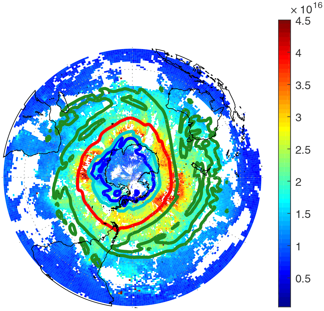
Figure 1Example of equivalent latitude contours for −70 (blue), −65 (light blue), −55 (red) and −40 (green) equivalent latitudes. The background colours are HNO3 total columns (daily mean for 21 July 2011, in molec cm−2).
As a general rule, we find larger concentrations in the Northern Hemisphere, for the entire latitudinal range shown here (40–90 eqlat). The hemispheric difference in HNO3 maximum concentrations can be partly attributed to the hemispheric asymmetry of the Brewer–Dobson circulation associated with the many topographical features in the Northern Hemisphere compared to the Southern Hemisphere. As a result, the Northern Hemisphere has a more intense planetary wave activity, which strengthens the deep branch of the Brewer–Dobson circulation. This also has a direct effect on the latitudinal mixing processes, which usually extend into the Arctic polar region, but less so into the Antarctic due to a stronger polar vortex (Mohanakumar, 2008; Butchart, 2014).
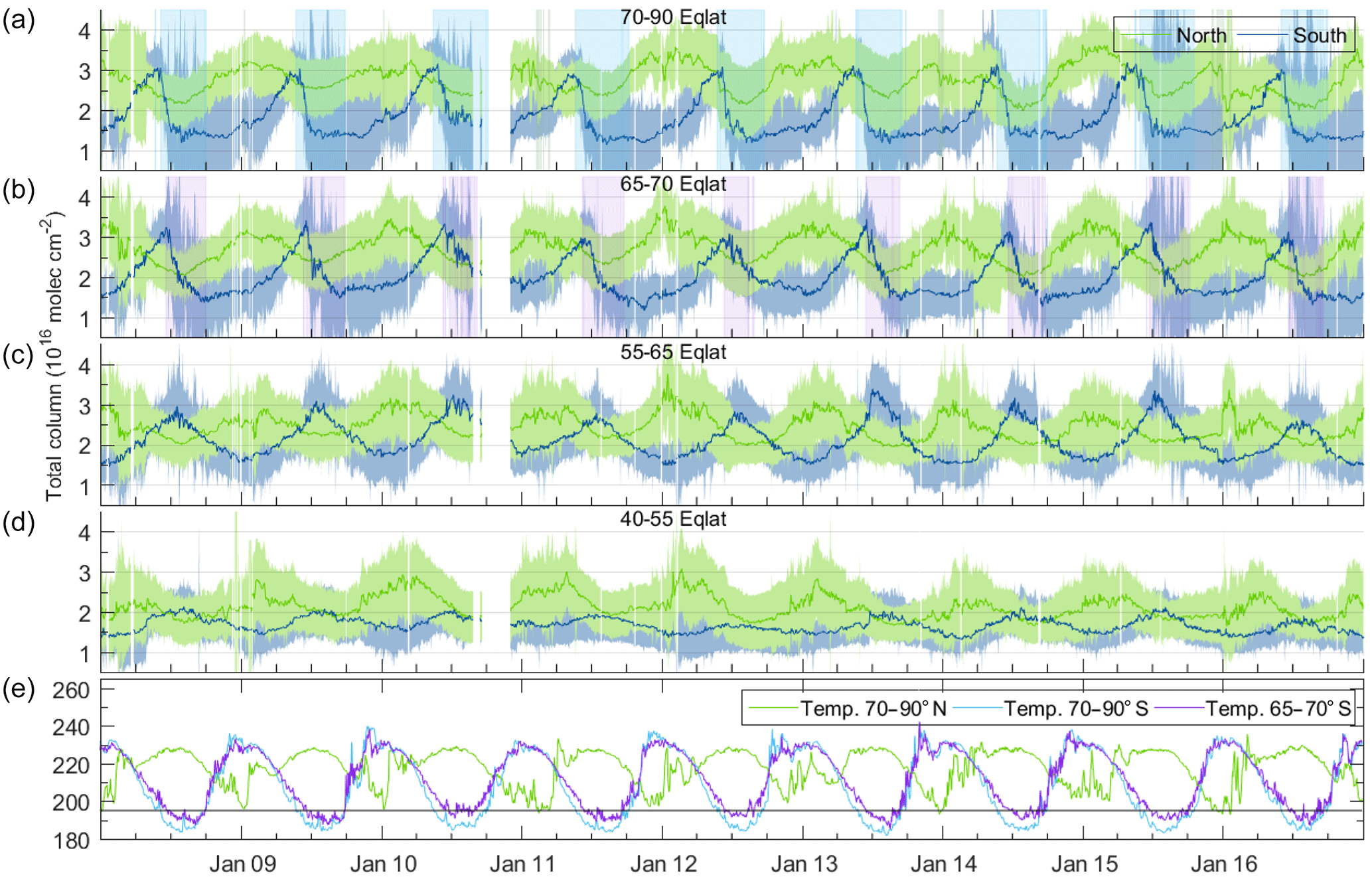
Figure 2(a–d) HNO3 total columns time series for the years 2008–2016, for equivalent latitude bands 70–90, 65–70, 55–65 and 40–55, north (green) and south (blue). Vertical shaded areas are the periods during which the average temperatures are below TNAT in the north (green) and south (blue) 70–90∘ band, and in the south (purple) 65–70∘ band. Note that the large period without data in 2010 is when there was a low amount of data distributed by EUMETSAT (see Sect. 2). (e) Daily average temperatures time series (in K) taken at the altitude of 50 hPa for the equivalent latitude bands 70–90∘ N (green) and South (blue) and 65–70∘ S (purple). The horizontal black line represents TNAT, i.e. the 195 K line.
Beyond hemispheric asymmetry, we also find that HNO3 columns are generally larger at higher latitudes, with total column maxima between 3.0 × 10¹⁶ and 3.7 × 10¹⁶ molec cm−2 in the equivalent latitudes bands 70–90, 65–70 and 55–65∘, and lower at around 2.2 × 10¹⁶ molec cm−2 in the 40–55∘ band, especially for the Southern Hemisphere. This latitudinal gradient of HNO3 has been previously documented (e.g. Santee et al., 2004; Urban et al., 2009; Wespes et al., 2009; Ronsmans et al., 2016) and can mainly be explained by the larger amounts of NOy at high latitudes due to a larger age of air and the NOy partitioning favouring HNO3. An interesting feature observable in Fig. 2 is the different behaviour of the three highest latitude regions with regard to the polar stratospheric cloud formation threshold in the Southern Hemisphere. The denitrification process that occurs with the condensation and sedimentation of PSCs (see e.g. Wespes et al., 2009; Manney et al., 2011 and Ronsmans et al., 2016 for further details) is obvious in the 70–90∘ S region (blue curve in Fig. 2a), with a systematic and strong decrease in HNO3 total columns (from 3.3 × 10¹⁶ to 1.5 × 10¹⁶ molec cm−2) starting within 12 to 25 days after the stratospheric temperature reaches the threshold of 195 K (start of the blue shaded areas). The loss of HNO3 therefore usually starts around the beginning of June in the Antarctic and the concentrations reach their minimum value within one month. They stay low at 1.4 × 10¹⁶ molec cm−2 until mid-November (with a slight gradual increase to 1.7 × 10¹⁶ molec cm−2 quite often seen during the two following months), and start to increase again during January, i.e. between 2.5 and 3 months after the polar stratospheric temperatures are back above the NAT formation threshold. The same pattern can be observed in the 65–70∘ S equivalent latitude region. However, a delay of approximately 1 month exists for the start of the steepest decrease in HNO3 columns, which appears to be more gradual than in the 70–90∘ S regions (3 months to reach minimum values, starting in July). The minimum and plateau column values are thus reached by the end of September; they remain higher than at the highest latitudes, with values staying at around 1.7 × 10¹⁶ molec cm−2. The delayed and less severe loss of HNO3 in the 65–70∘ S band confirms that the denitrification process spreads from the centre of the polar vortex, where the lowest temperatures are reached first (McDonald et al., 2000; Santee et al., 2004; Lambert et al., 2016). This spreading from the centre also leads to slightly higher concentrations for the maxima in the 65–70∘ S eqlat band (mean of maxima of 3.26 × 10¹⁶ versus 3.11 × 10¹⁶ molec cm−2 in the 70–90∘ S eqlat band). The delayed decrease in HNO3 in the outer parts of the vortex (i.e. in the 65–70∘ S eqlat band) can thus be attributed to the later appearance of PSCs in this region (see Fig. 2b purple shaded areas). By the end of December, when the vortex has started breaking down (e.g. Schoeberl and Hartmann, 1991; Manney et al., 1999; Mohanakumar, 2008), the total columns in both eqlat bands become homogenized and reach the same range of values (1.7 × 10¹⁶ molec cm−2).
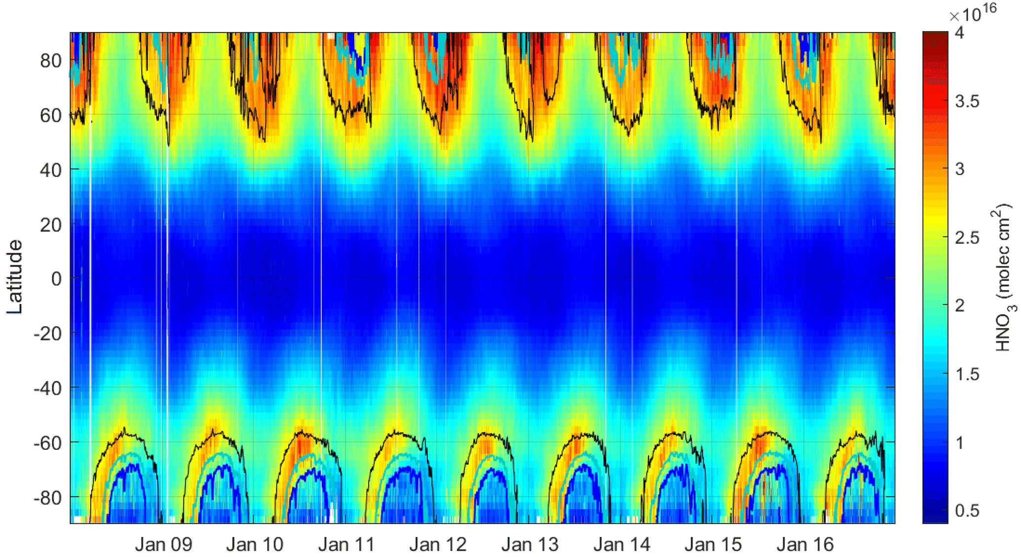
Figure 3Zonally averaged daily HNO3 total columns distribution over 2008–2016, expressed in molec cm−2. The lines represent potential vorticity contours at a potential temperature of 530 K (5 (black), 8 (cyan) and 10 (blue) × 10−6 K m2 kg−1 s−1) which correspond to the equivalent latitudes contours illustrated in Fig. 1.
If the decrease is slower at 65–70 eqlat, this is not the case for the recovery, with the build-up of concentrations starting roughly at the same time as for the 70–90∘ S eqlat band, hence resulting in a shorter period of denitrified atmosphere in the 65–70∘ S band. These results agree well with previous studies by McDonald et al. (2000) and Santee et al. (2004) for earlier years. However, the recovery of the HNO3 total columns is very slow compared to other species, namely O3, for which concentrations return to usual values within 2 months (i.e. in December) after PSCs have disappeared. In fact, the HNO3 columns stay low until well after the September equinox and are only subject to a slow increase starting 2 months later (in early December) with concentrations back to pre-denitrification levels by May. While more persistent local temperature minima staying below 195 K could explain part of this late recovery, we hypothesize that it is mainly due to a combination of two factors: (1) the significant sedimentation of PSCs towards the lower atmosphere during the winter, such that few PSCs remain available to release HNO3 under warmer temperatures (Lowe and MacKenzie, 2008; Kirner et al., 2011; Khosrawi et al., 2016); and (2) the effective photolysis of HNO3 and NO3 in spring and summer under prolonged sunlight conditions, mainly at the highest latitudes, which respectively increase the HNO3 sink and reduce the chemical source (because NO3 cannot react with NO2 to produce N2O5, Solomon, 1999; Jacob, 2000; McDonald et al., 2000). The increase observed in March, at the start of the winter, can in turn be explained by a reduction in the number of hours of sunlight (implying less photodissociation), as well as by diabatic descent, which brings HNO3-rich air to lower altitudes.
It is worth noting that the two regions previously mentioned (inner and outer vortex) have been observed to behave differently; the inner vortex (70–90∘ S) undergoes strong internal mixing whereas the outer vortex (65–70∘ S), isolated from the vortex core, experiences little mixing of air. This, combined with a cooling of the stratosphere, could lead to increased PSC formation and further ozone depletion (Lee et al., 2001; Roscoe et al., 2012).
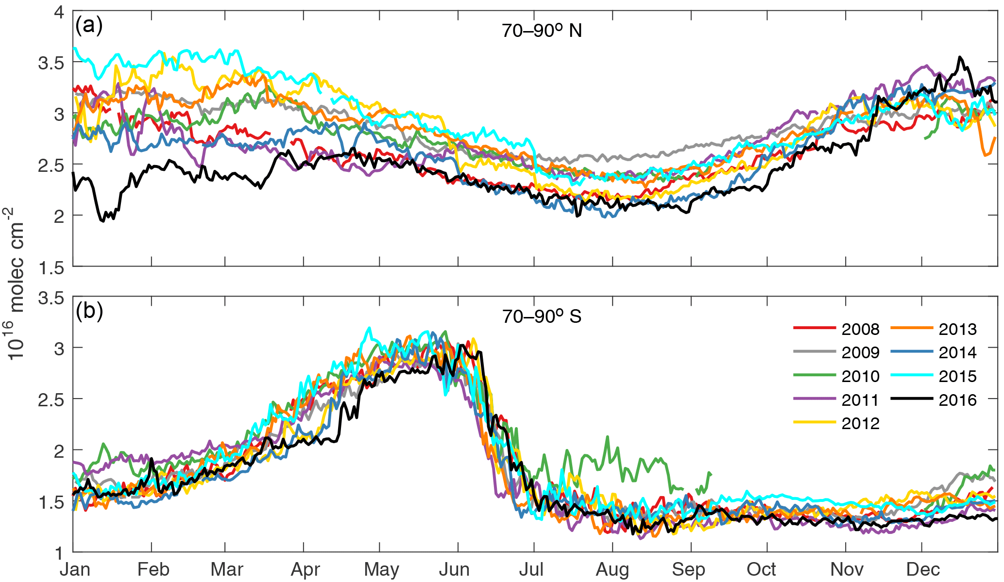
Figure 4For northern (a) and southern (b) 70–90 equivalent latitude bands: HNO3 total columns time series for the years 2008 to 2016 in molec cm−2. Note that the y axis limits differ between the two plots.
Regarding the HNO3 columns in the 55–65∘ S eqlat band, which comprises the vortex rim, or “collar” (Toon et al., 1989), it is evident from Fig. 2c that they are not affected by denitrification, which is in agreement with previous observations (e.g. Santee et al., 1999; Wespes et al., 2009; Ronsmans et al., 2016). In fact, we show that columns in this particular band keep increasing when temperatures at higher latitudes start decreasing, to reach maximum values of about 3.4 × 10¹⁶ molec cm−2 in June–July; this is due to a change in NOy partitioning towards HNO3, which is in turn due to less sunlight in this period compared to summer. Also inducing increased concentrations during the winter at high latitudes is the diabatic descent occurring inside the vortex when temperatures decrease. This downward motion of air enriches the lower stratosphere with HNO3 coming from higher altitude (Manney et al., 1994; Santee et al., 1999), yielding higher column values which are, in this eqlat band, not affected by denitrification. The slow decrease in HNO3 starting in August and leading to minimum values in January is related to the combined effect of increased photodissociation and mixing with the denitrified polar air masses which are no longer confined to the polar regions. Finally, as previously mentioned, the 40–55∘ S eqlat band records lower column values throughout the year (generally below 2 × 10¹⁶ molec cm−2) and a much less pronounced seasonal cycle.
High latitudes in the Northern Hemisphere do not usually experience denitrification, mostly because the temperatures, while frequently showing local minima below 195 K, rarely reach the PSC formation threshold over broad areas and for long time spans (see Fig. 2 for average temperatures, light green vertical areas). A few years stand out, however, with exceptionally low stratospheric temperatures. This is especially the case of the 2011 (Manney et al., 2011), 2016 and, to some extent, 2014 Arctic winters. During these three winters, temperatures dropped below the 195 K threshold over a broader area and stayed low for a longer period than usual. Lower concentrations of HNO3 were recorded as a consequence, especially in the northernmost equivalent latitude band (see Fig. 2). The winter 2016 recorded exceptionally low temperatures in particular, which led to large denitrification and significant ozone depletion (Manney and Lawrence, 2016; Matthias et al., 2016). The denitrification that occurred in the northern polar regions affected a smaller area than is generally observed in the Southern Hemisphere; the columns in the 65–70∘ N eqlat band in particular do not show a significant decrease.
Figure 3, which consists of the time series of the zonally averaged distribution of HNO3 retrieved total columns, illustrates all of these features particularly well: it highlights the low and constant columns between −40 and 40 degrees of latitude, the marked annual cycle at mid to high latitudes and the systematic and occasional (2011, 2014, 2016) loss of HNO3 during denitrification periods in the high latitudes of the Southern and Northern hemispheres respectively, which are highlighted by the iso-contours of potential vorticity at ±10 × 10−6 K m2 kg−1 s−1 (dark blue).
In order to give further insights into the interannual variability of HNO3 in polar regions, Fig. 4 shows the seasonal cycle for each individual year from 2008 to 2016 for eqlat 70–90 in the northern (Fig. 4a) and the southern (Fig. 4b) hemispheres. July and August of 2010 stand out in the Antarctic, with high and variable columns recorded by IASI. This is a consequence of a mid-winter (mid-July) minor sudden stratospheric warming (SSW) event, which induced a downward motion of air masses and modified the chemical composition of the atmosphere between 10 and 50 hPa until at least September (de Laat and van Weele, 2011; Klekociuk et al., 2011). The principal effect of this sudden stratospheric warming was to reduce the formation of PSCs (which stayed well below the 1979–2012 average WMO, 2014) and hence reduce denitrification. This is shown by an initial drop in HNO3 columns in June, as is usually observed in other years but then by an increase in HNO3 columns when the SSW occurs. These results confirm those previously obtained by the Aura MLS during that particular winter and reported in the World Meteorological Organization (WMO) Ozone Assessment of 2014 (see Fig. 6-3 in WMO, 2014). Apart from these peculiarities for the year 2010, all years seem to coincide quite well in terms of seasonality in the Southern Hemisphere (bottom panel, Fig. 4). The timing of the HNO3 steep decrease in particular is consistent from one year to another.
The Northern Hemisphere high latitudes (top panel, Fig. 4) show more interannual variability than in the south, especially during the winter because of the unusual denitrification periods observed in 2011 (purple), 2014 (blue) and 2016 (black) in January (concentrations as low as 2.2 × 10¹⁶ molec cm−2 in 2016). In contrast to the winter, the summer columns are more uniform from one year to another with values around 2.1 × 10¹⁶ to 2.8 × 10¹⁶ molec cm−2.
4.1 Multi-variable linear regression
In order to identify the processes responsible for the HNO3 variability observed in the IASI measurements, we use a multivariate linear regression model featuring various dynamical and chemical processes known to affect HNO3 distributions. We strictly follow the methodology used by Wespes et al. (2016) for investigating O3 variability; in particular, we use daily median HNO3 total columns. These are fitted with the following model:
where t is the day in the time series, cst is a constant term, the y terms are the regression coefficients for each variable, , and YNorm,i(t) refers to the chosen explanatory variables Y, which are normalized over the period of IASI observations (2008–2016) following
with Ymax and Ymin being the maximum and minimum values of the variable time series (before subtraction of the median, Ymedian). The terms a1 and b1 in Eq. (1) are the coefficients accounting for the annual variability in the atmosphere. They represent mainly the seasonality of the solar insolation and of the meridional Brewer–Dobson circulation, which is a slow stratospheric circulation redistributing the tropical air masses to extra-tropical regions (Mohanakumar, 2008; Butchart, 2014; Konopka et al., 2015).
The regression coefficients are estimated by the least squares method. The standard error (σe) of each proxy is calculated based on the regression coefficients and is corrected in order to take the autocorrelation uncertainty into account (Knibbe et al., 2014; Wespes et al., 2016):
where Y is the matrix of explanatory variables of size n×m, n is the number of daily measurements and m the number of fitted parameters. HNO3 is the nitric acid column, y the vector of regression coefficients and φ is lag-1 autocorrelation of the residuals.
4.2 Iterative selection of explanatory variables
The choice of variables included in the model is made using an iterative elimination procedure; all variables are tested based on their importance for the regression (Mäder et al., 2010). At each iteration, the variable with the largest p value (and outside the confidence interval of 95 %) is removed, until only the variables relevant for the regression remain, i.e. variables with a p value smaller than 0.05. This selection algorithm is applied on each band of equivalent latitude (or grid cell, for the global distributions shown below) and thus yields a different combination of variables, depending on the equivalent latitude region considered.
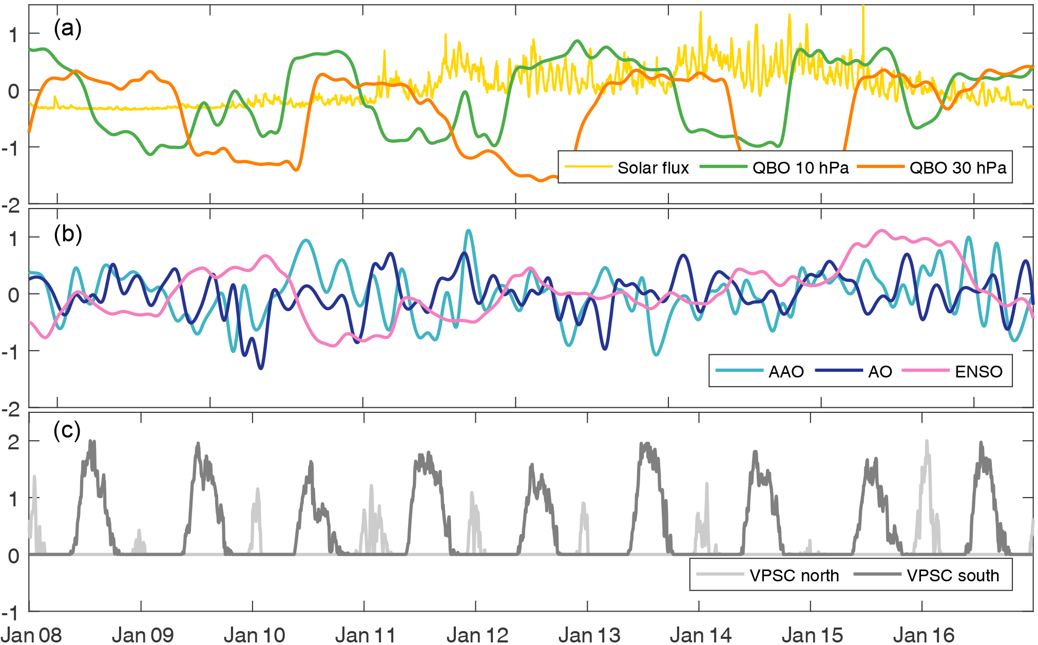
Figure 5Normalized proxies over the IASI observations period (2008–2016). (a) Solar flux (yellow), QBO at 10 hPa (green) and QBO at 30 hPa (orange). (b) Antarctic Oscillation (light blue), Arctic Oscillation (dark blue) and Multivariate ENSO Index (MEI, pink). (c) VPSC proxy in the Northern Hemisphere (light grey) and in the Southern Hemisphere (dark grey).
4.3 Variables used for the regression
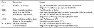
Given the strong relationship between the O3 and HNO3 chemistry and variability (Solomon, 1999; Neuman et al., 2001; Santee et al., 2005; Popp et al., 2009) and the novelty of applying such a regression study in an HNO3 dataset, we consider the major and well known drivers of total O3 variability here, namely a linear trend, harmonic terms for the annual variability and geophysical proxies for the solar cycle, the QBO, the ENSO phenomenon and the Arctic (AO) and Antarctic oscillations (AAO) for the Northern and Southern hemispheres, respectively. Considering the short length of the time series, however, the linear trend did not yield any significant result and, recalling that the aim of the paper is not to derive long term trends, this aspect will not be discussed further. In addition, a proxy for the volume of polar stratospheric clouds is included to account for the effect of the strong denitrification process during the polar night (cf. Sect. 3). All the proxies are shown in Fig. 5 and described in more details hereafter. The source for each proxy is also provided in Table 1.
4.3.1 Solar flux (SF)
As a proxy for the solar activity we use the 10.7 cm solar flux (F10.7), which is a radio flux that varies daily and correlates to the number of sunspots on the solar disk (Covington, 1948; Tapping and DeTracey, 1990; Tapping, 2013). The data set used here is the adjusted flux that takes the changing earth–sun distance into account. The solar cycle directly influences the partitioning between NOy (produced by the N2O + O1D reaction) and HNO3 through the quantity of sunlight available, and has been known to affect the dynamics and to influence the O3 response in the lower stratosphere (e.g. Hood, 1997; Kodera and Kuroda, 2002; Hood and Soukharev, 2003; Austin et al., 2007).
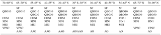
Table 2Set of variables retained by the selection algorithm for each equivalent latitude band.
4.3.2 Quasi-biennial oscillation (QBO)
The QBO is one of the main process regulating the dynamics of the tropical atmosphere (e.g. Baldwin et al., 2001; Sioris et al., 2014). It is driven by vertically propagating gravity waves, which lead to an oscillation between stratospheric winds blowing from the east (easterlies) and west (westerlies), occurring over a mean period of about 28–29 months (e.g. Hauchecorne et al., 2010; Schirber, 2015). The effect of the QBO on the distribution of chemical species is significant, especially in equatorial regions where both a direct effect due to the changing winds and an indirect effect via its influence on the Brewer–Dobson circulation, affect, for example, the distribution of ozone (e.g. Lee and Smith, 2003; Mohanakumar, 2008; Frossard et al., 2013; Knibbe et al., 2014). Two monthly time series of QBO at two different pressure levels (30 and 10 hPa) from ground-based measurements in Singapore were considered in the present study, in order to take the differences in phase and shape of the QBO signal in the upper and lower stratosphere into account.
4.3.3 Multivariate ENSO Index (MEI)
The Multivariate ENSO Index is a metric that quantifies the strength of the El Niño–Southern Oscillation; it is computed based on the measurement of six variables over the tropical Pacific: sea-level pressure, zonal and meridional winds, sea surface temperature, surface air temperature, and cloudiness fraction (Wolter and Timlin, 1993, 1998). The ENSO phenomenon, even though it is a tropospheric process (mainly sea surface temperature contrasts), also affects stratospheric circulation. Previous studies have shown the impact of El Niño/La Niña oscillation on stratospheric transport processes and the generation of Rossby waves, which in turn modulate the strength of the polar vortex (e.g. Trenberth et al., 1998; Newman et al., 2001; Garfinkel et al., 2015) and affect O3 in the stratosphere (e.g. Randel et al., 2009; Lee et al., 2010; Randel and Thompson, 2011).
4.3.4 Arctic Oscillation and Antarctic Oscillation
The AO and AAO are included in the regression in order to represent the atmospheric variability observed in the Northern and Southern hemispheres, respectively (Gong and Wang, 1999; Kodera and Kuroda, 2000; Thompson and Wallace, 2000). They are constructed from the daily geopotential height anomalies in the 20–90∘ region, at 1000 mb (for the Northern Hemisphere) and 700 mb (for the Southern Hemisphere). Each index (AO or AAO) is considered only in the hemisphere it is related to, while both indices are included for equatorial latitudes. The impact of these oscillations on O3 distributions has been demonstrated in several studies (e.g. Rieder et al., 2013; Wespes et al., 2016). We may expect a similar influence on the HNO3 distributions, particularly because, even though they are tropospheric features, their phase and intensity affect the atmospheric circulation, and in particular the Brewer–Dobson Circulation, up to the stratosphere (Miller et al., 2006; Chehade et al., 2014).
4.3.5 Volume of polar stratospheric clouds (VPSC)
The very low temperatures recorded during the winter in the polar stratosphere inside the vortex lead to the formation of PSCs, which are composed of nitric acid di- or trihydrates (NAD or NAT), supercooled ternary HNO3 ∕ H2SO4 ∕ H2O solutions (STS) or water ice (H2O) (e.g. Wang and Michelangeli, 2006; Drdla and Müller, 2010). Here, we consider only the NAT particles (HNO3 ⋅ (H2O)3) for the PSCs, which are ubiquitous (and often mixed with STS) (Voigt et al., 2000; Pitts et al., 2009; Lambert et al., 2016). The other forms of PSCs are expected to influence the variability in gas-phase HNO3 to a much lesser extent (von König et al., 2002).
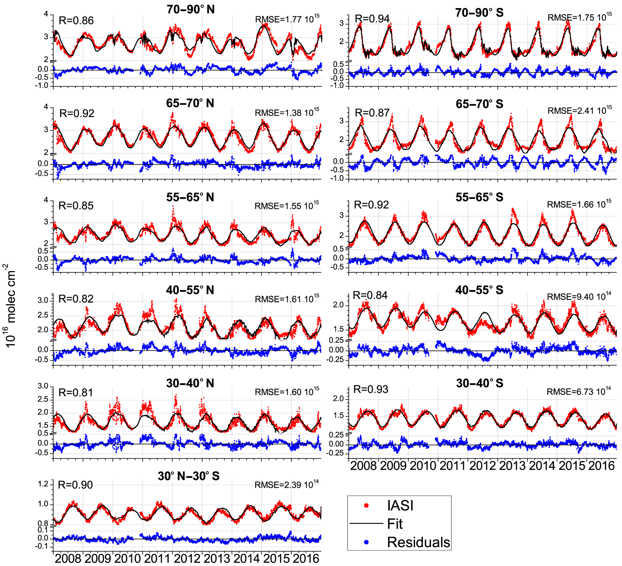
Figure 6IASI HNO3 total columns (red dots) for each of the equivalent latitude bands and the associated fitted model (black curves). The residuals are in blue, and the horizontal black line represents the zero residual line. For each equivalent latitude band, the correlation coefficient (R) between the observations and the model fit is given in the top left corner, and the root mean square error (RMSE) in the top right corner.
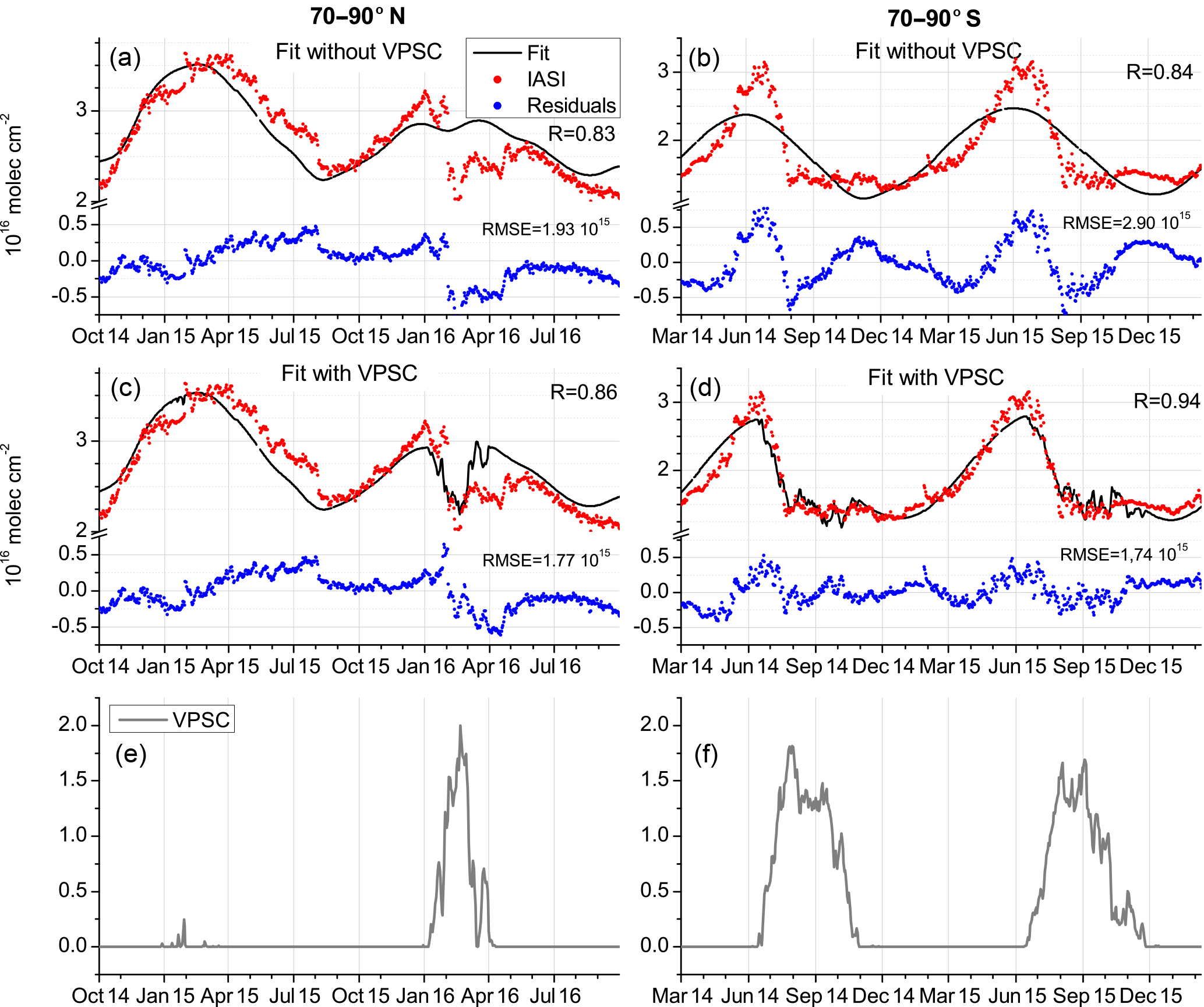
Figure 7For north (a, c, e) and south (b, d, f) equivalent latitude bands 70–90∘: (a, b) total columns (in 1016 molec cm−2) of IASI observations (red) and the regression fit without the VPSC proxy (black), for a subset of the time series, zooming on denitrification periods. The correlation coefficients between the fit and the IASI data (R) are displayed, as well as the root mean square error (RMSE). (c, d) Same as top panels but for the fit with the VPSC proxy. (e, f) Normalized VPSC proxy. Note the different time and value ranges between the two hemispheres.
The proxy we use here for the NAT is the volume of air below TNAT
(195 K), which depends on nitric acid concentrations, water vapour and
pressure (Hanson and Mauersberger, 1988; Wohltmann et al., 2007). The temperatures needed to compute
the quantity are based on ERA-Interim reanalyses, and the HNO3 and
H2O profiles are taken north and south of 70∘ from an MLS
climatology. The proxy is calculated with a supersaturation of HNO3 over
NAT of 10, roughly corresponding to 3 K supercooling
(Hoyle et al., 2013; Lambert et al., 2016; Wohltmann et al., 2017). It should be noted that this
proxy was not included in the regression outside of the polar regions. Inside
the polar regions (eqlat bands 70–90 north and south), it was included and
subject to the selection algorithm.
Finally,
for the sake of completeness, proxies accounting for the potential vorticity
(PV) and for the Eliassen–Palm flux (EPflux) were also tested in order to
take more precise patterns of the stratospheric dynamics and the
Brewer–Dobson circulation into account. Various levels for the QBO were also
tested. However, none of these proxies lead to a significant improvement of
the residuals or the correlation coefficients, and their signal is therefore
embedded here in the harmonic terms. For these reasons, they will not be
discussed further.
4.4 Results
The results are presented in two ways: latitudinally averaged time series (eqlat bands) are used to analyse the performances of the fit in terms of correlation coefficients and residuals, with a focus on polar regions; the performance of the model is then analysed in terms of global distributions (with the regression applied to every grid cell) and the spatial distribution of the fitted proxies is detailed.
4.4.1 HNO3 fits for equivalent latitude bands
For each eqlat band, the variables retained by the selection procedure (see Sect. 4.2) are listed in Table 2. Most variables are retained everywhere, except for the solar flux which is rejected in the polar latitudes (70–90∘ N and S). The QBO30 is also excluded in the southern polar regions (65–90∘ S) and the MEI in the northern polar regions (65–90∘ N). Finally, the AO and AAO are excluded in the 65–70∘ N and in the 70–90∘ S bands, respectively.
The results from the multivariate regression are presented in Fig. 6 for each band of equivalent latitude. The model reproduces the measurements well, with correlation coefficients between 0.81 (in the 30–40∘ N eqlat band) and 0.94 (in the 70–90∘ S eqlat bands). Most major features (seasonal and interannual variabilities) are reproduced by the regression model. The residuals range between 1.74 × 10¹⁰ and 9.44 × 10¹⁵ molec cm−2, with better results for the 30∘ N–30∘ S equivalent latitude band (Root Mean Square Error (RMSE) of 2.39 × 10¹⁴ molec cm−2) and worse fits for the 65–70∘ S band (RMSE of 2.41 × 10¹⁵ molec cm−2). Following the comparison between the fits and the observational data, some features can be highlighted:
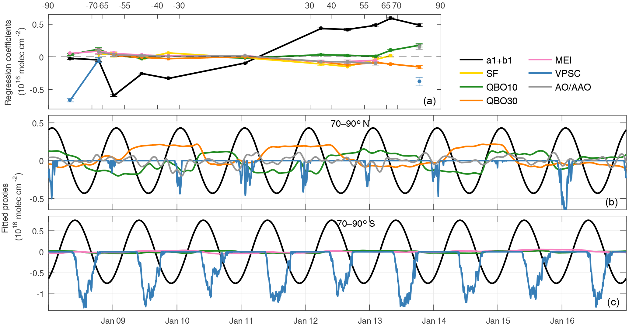
Figure 8(a) Regression coefficients (xi) and their standard error (σe, error bars, calculated by Eq. 3) for the selected variables in each equivalent latitude band (each data point is located in the middle of its corresponding eqlat band). (b, c) Fitted signal of the proxies in the eqlat bands 70–90 north (b) and south (c) for the variables selected. They are calculated as [xi⋅Xi] with Xi the normalized proxy and xi the regression coefficient calculated by the regression model.
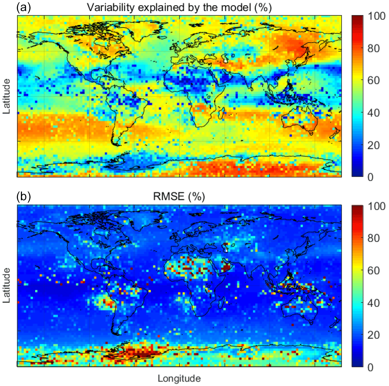
Figure 9(a) Fraction (%) of the HNO3 variability in the IASI observations explained by the regression model, and calculated as . (b) Root Mean Square Error (RMSE) calculated for each grid cell as and expressed in %.
-
The high daily variability recorded in the data during the winter for both polar regions is not captured very well by the regression fit. Indeed, we find that the residuals are largest in this period, especially in the Southern Hemisphere during the denitrification period of each year (from June until September approximately), mostly because of the high variability of the vortex itself. We find an average standard deviation of 1.44 × 10¹⁶ molec cm−2 (average of the standard deviation during the denitrification periods over the 9 years of observation), as opposed to a mean standard deviation of 8.30 × 10¹⁵ molec cm−2 for the periods between the denitrification seasons. In the Northern Hemisphere, the day-to-day variability is largest during winter as well, due to the vortex building up, and this causes larger residuals for the corresponding months (see December through March of each year, top left panel of Fig. 6, with an average standard deviation of 7.97 × 10¹⁵ molec cm−2 compared to 7.26 × 10¹⁵ molec cm−2 for other months). It is important to stress that these larger residuals are obtained in the polar regions despite the fact that a VPSC proxy was used. In Fig. 7 we show, however, that the regression model performs worse in polar regions if the proxy is neglected, as also discussed below.
-
Even though the high variability during the denitrification periods is not exactly reproduced, the amplitude of the decrease in HNO3 occurring in the southern polar region is captured accurately by the regression model. Figure 7 shows a zoomed in area of Fig. 6 to better highlight the model performance during the denitrification periods; the regression was tested without (top panels) and with (middle panels) the VPSC proxy, for the 70–90∘ N (left panels) and the 70–90∘ S (right panels) eqlat bands. The steep slope observed at the start of the low temperatures is captured by the model when the proxy for the VPSC is included (Fig. 7) and the correlation coefficients are improved for both hemispheres (from 0.83 to 0.86 in the 70–90∘ N and from 0.84 to 0.94 in the 70–90∘ S eqlat band). In the 65–70∘ S eqlat band however, as previously described in Sect. 3, the HNO3 columns continue to increase after the formation of PSCs has started in the 70–90∘ S eqlat band. This translates to a lag between the observations in the 65–70∘ S eqlat band and the fit, in which the drop of HNO3 concentrations occurs earlier than in the IASI observations. This is explained by the fact that the VPSC proxy is based on temperatures and composition poleward of 70∘. It induces a lower correlation coefficient (0.87) and higher RMSE (2.41 × 10¹⁵ molec cm−2). A proxy adapted to this eqlat band should be used in further studies in order to represent the conditions in this particular region of the vortex.
-
The high maxima seen in the IASI time series, mostly from mid-April through to the end of May in the Southern Hemisphere, and from mid-December through early February in the Northern Hemisphere, are not that well reproduced by the regression model. In fact, the model fails to capture the highest columns during the winters of each hemisphere. In the same way, a few pronounced lows recorded by IASI, especially those in the Northern polar regions (mid-June to early October 2014 and 2016, for instance) are not captured by the model.

Figure 10Time evolution of IASI HNO3 (red) and GOME-2 NO2 (green) from 2008 to 2015 for Africa south of the Equator (5–20∘ S, 10–40∘ E). Both HNO3 and NO2 columns are expressed in molec cm−2. The NO2 data are tropospheric columns (Valks et al., 2011) and are obtained from ftp://atmos.caf.dlr.de/. Note that the ranges differ between the two y axes.
Figure 8 shows the regression coefficients of each variable in each equivalent latitude band (top panel). The two bottom panels show the signal of the fitted proxies, calculated by multiplying the proxy by its regression coefficient. Only the variables retained by the selection algorithm are shown and discussed. From Fig. 8a, it can be seen that all proxies are significant, with errors smaller than the coefficients for all eqlat bands. It is clear that annual variability is predominant at all latitudes. From the two bottom panels, we also see the large influence of the VPSC in the regression for the polar regions. Their signal is, as expected, larger in the Southern Hemisphere where it reaches −1.3 × 10¹⁶ molec cm−2, which can be compared to maximum values of around −0.4 × 10¹⁶ molec cm−2 in the Northern Hemisphere. A noteworthy difference is found for the year 2016 where the VPSC signal reached −0.7 × 10¹⁶ molec cm−2 during the exceptionally cold Arctic winter. While the PSCs have significantly affected HNO3 distributions in the winters of 2011, 2014 and 2016 in the Arctic, their influence during other years may contribute to the high variability recorded in the observations (see first highlighted feature above). Other proxies show relatively large signals and their global distribution will be discussed further in Sect. 4.4.3.
4.4.2 Global model assessment with regard to the HNO3 variability
To assess the model's ability to reproduce the measurements, Fig. 9a shows the percentage of the HNO3 variability seen by IASI that is explained by the regression model. The fraction is calculated as the difference between the standard deviation of the fit and the observations and is expressed as a percentage. We find that much of the observed variability can be explained by the model in the Southern Hemisphere (generally between 50 and 80 %). The southern mid-latitudes and the polar regions are particularly well modelled (70–80 %), except in Antarctica above the ice shelves. The Northern Hemisphere HNO3 variability is reasonably well explained by the model, particularly above 40∘ of latitude, with percentages ranging between 50 and 80 %, although some continental areas (Northern part of inner Eurasia above Kazakhstan and the West Siberian plains) stand out with percentages below 40 %. The region with the largest unexplained fraction of variability is the intertropical band extending as far as 40∘ north. There, the fraction of HNO3 variability explained by the model reaches values as low as 20 %. These regions of low explained variability coincide quite well with the regions where high lightning activity is found, which produces large amounts of NOx in the troposphere (Labrador et al., 2004; Sauvage et al., 2007; Cooper et al., 2014). While the IASI instrument is usually not sensitive to tropospheric HNO3, it was found that large amounts of tropospheric HNO3 in the tropics could be detected. This is mainly owing to the lower contribution of the stratosphere in this region, and because the NOx produced by lightning is released in the high troposphere, where IASI has still reasonable sensitivity. This could consequently explain why the model is missing some of the variability recorded in the observational data. Another cause for the discrepancies between the observations and the model could be unaccounted sinks of HNO3, such as deposition in the liquid or solid phase and scavenging by rain. It should be noted that a small area of high explained variability is observed in Africa, just south of the Equator. The variability in this region is unexpectedly high in the IASI time series (Fig. 10) and we suggest that it could be influenced by biomass burning emissions of NO2, and subsequent oxidation to HNO3 with a delay of about 2 months (Fig. 10) (Scholes et al., 1996; Barbosa et al., 1999; Schreier et al., 2014). Indeed, the large vegetation fires in Africa every year around July emit the largest amounts of NOx (compared to large fires in South America, Australia and southeast Asia). Their influence translates to an over-representation of the annual term (up to −2 × 10¹⁵ molec cm−2) in the fitted model (although not clearly visible in Fig. 11 because of the colour scale chosen). This larger contribution of the annual variability thus yields a better agreement between the observations and the model in the tropical band. However, some of the interannual variability is missing due to the above-mentioned fires.
Fig. 9b depicts the global distribution of the RMSE of the regression expressed as a percentage. The errors are small everywhere (between 10 and 20 %) except in the Southern Hemisphere above Antarctica, and particularly above the ice shelves (mainly the Ross and Ronne ice shelves). We also find higher values above large desert areas (the Sahara, the Arabian, the Turkistan and the Australian deserts) as well as off the west coasts of South Africa and South America where persistent low clouds occur. Regions of low clouds or those characterized by emissivity features that are sharp (e.g. deserts) or seasonally varying (e.g. ice shelves) are known to cause problems for the retrieval of HNO3 using the IASI spectra (Hurtmans et al., 2012; Ronsmans et al., 2016).

Figure 11Global distributions ( grid) of the regression coefficients expressed in 1015 molec cm−2. The gray crosses are the cells where the proxy is not significant when accounting for autocorrelation (see Eq. 3). The white cells are where the proxy was not retained and the black cells represent a coefficient of 0. Note the different scales. The x axes are latitudes.
4.4.3 Global patterns of fitted parameters
Figure 11 shows the global distributions of the regression coefficients obtained after the multivariate regression, expressed in molec cm−2. All the variables are shown, with the areas where the proxy was not retained left blank. The contribution of each proxy to the HNO3 variability was also calculated for each grid cell as with Xi referring to each of the i explanatory variables X, and expressed as a percentage. Note that, although the distributions of the contribution of each proxy are not shown as a figure, the calculated percentage values are used in the following discussion (next 3 subsections) to quantify the influence of the fitted parameters.
The annual cycle
The annual cycle, represented by the terms a1 and b1, shows large regression coefficients (Fig. 11) and holds the largest part of the variability globally (up to 70 % in the northern and southern mid to high latitudes), as was previously evidenced in Fig. 8a. While the Brewer–Dobson circulation, which is embedded in these harmonic terms, influences the HNO3 variability to some extent (through its influence on the conversion of N2O to NOy in the tropics and through the transport of NOy-rich air masses towards the polar regions and subsequent transformation into HNO3), the impact of the seasonality of the solar insolation is also likely to largely influence the annual seasonality, especially in the mid- to high latitudes. The increasing columns recorded during the winter in both polar regions can be explained by the combination of three processes: first, at low temperatures, HNO3 is formed by heterogeneous reactions between N2O5 and H2Oaerosol and between ClONO2 and H2Oaerosol or HClaerosol, which add to the main source gas-phase reaction OH + NO2 + M → HNO3; second, while the source reactions of HNO3 are still active, the loss reactions (HNO3 photolysis and its reaction with OH) are significantly slowed down during the winter (Austin et al., 1986; McDonald et al., 2000; Santee et al., 2004); and third, as is mentioned in Sect. 3, with the decrease of temperatures in the polar stratosphere, the winds inside the polar vortex gain intensity and induce a strong diabatic downward motion of air with little latitudinal mixing across the vortex boundary. This descending air from the upper stratosphere enriches the lower stratosphere in HNO3 (Schoeberl and Hartmann, 1991; Manney et al., 1994; Santee et al., 1999).
The solar cycle, MEI, AO/AAO and QBO
The solar flux, ENSO index and Arctic and Antarctic Oscillation (Fig. 11) all have a similar influence in terms of magnitude (between −2.5 × 10¹⁵ and 2.5 × 10¹⁵ molec cm−2), although with different spatial patterns. The influence of the solar flux is positive in the northern polar latitudes and in the tropical and southern mid-latitudes. It is close to zero or negative elsewhere. While previous studies showed a positive signal globally in the low stratosphere for the response of O3 to the solar cycle (Hood, 1997; Soukharev and Hood, 2006), our results for the mid to high northern latitudes suggest opposite behaviour (negative signal) for HNO3. However, the positive contribution of the solar cycle on the HNO3 variation in the tropical and southern mid-latitude stratosphere is in line with the O3 response previously reported (Soukharev and Hood, 2006; McCormack et al., 2007; Frossard et al., 2013; Maycock et al., 2016). Note also that the strong negative signal observed above the ice shelves of western Antarctica is most probably due to the drawback of using a constant emissivity for ocean surfaces for all seasons (e.g. even when the ocean becomes frozen). For this reason, the regression coefficients in this area will not be discussed further.
The MEI shows a negative signal above the northern polar regions and in the eastern parts of the Pacific and Atlantic oceans (especially west of South Africa). A positive signal is observed above Australia and above the southern polar regions. Overall, the MEI influence is quite small, which is not surprising considering that it affects mostly the tropospheric circulation, where IASI is less sensitive. Its signature is nonetheless visible and significant in the eastern Pacific, where it contributes to up to 30% of the HNO3 variability, and in the mid-latitudes of the Northern Hemisphere. The east–west gradient is in good agreement with chemical and dynamical effects of El Niño on O3, and with previous studies that showed the same patterns for the influence of the MEI on O3 (Hood et al., 2010; Rieder et al., 2013; Wespes et al., 2017).
The Arctic Oscillation (AO) signal is stronger, especially above the Atlantic Ocean, with a positive signal above eastern Canada and Greenland and between the north of eastern Africa and Florida. Except for those two regions, the AO contributes at mid to high latitudes of the Northern Hemisphere with a negative signal, which contributes 10–20 % to the HNO3 variability. The corresponding proxy for the Southern Hemisphere (AAO) is also significant, with a strong positive signal above the vortex rim and a negative signal above Antarctica. These results are in agreement with previous studies that showed that, for O3, both the Arctic and Antarctic oscillations (also called “annular modes”) are leading modes of variation in the extratropical atmosphere (Weiss et al., 2001; Frossard et al., 2013; de Laat et al., 2015; Wespes et al., 2017). Both the AO and the AAO strongly influence the circulation up to the lower stratosphere and represent, particularly in the Southern Hemisphere, fluctuations in the strength of the polar vortex (Thompson and Wallace, 2000; Jones and Widmann, 2004; van den Broeke and van Lipzig, 2004). This further shows the similarity in the behaviour of O3 and HNO3.
The QBO has a generally small influence on the distributions with, however, some contribution (up to 30 %) in the equatorial band as expected (Baldwin et al., 2001; Solomon et al., 2014). As previously mentioned, several tests were performed (not shown here) with the QBO taken at other atmospheric pressure levels (namely 20 and 50 hPa), and similar results were obtained. Even though the QBO is a tropical phenomenon, its effects extend as far as the polar latitudes, through the modulation of the planetary Rossby waves (e.g. Holton and Tan, 1980; Baldwin et al., 2001). Because there are more topographical features in the Northern Hemisphere than in the Southern Hemisphere, these waves have a larger amplitude and can influence the Arctic stratospheric temperatures and hence the vortex formation. While the exact mechanism for the extratropical influence of the QBO is not exactly understood (Garfinkel et al., 2012; Solomon et al., 2014), it seems the large positive and negative signals observed in the northern high latitudes in Fig. 11 can indeed be attributed to the modulation of the Rossby waves by the oscillation in the meridional circulation. This was also observed for O3 in studies such as Wespes et al. (2017).
VPSC
The annual cycle, which is the dominant factor for HNO3 variability at all latitudes, leading to the build-up of concentrations during the winter, is interrupted in the southern polar regions, particularly in the 70–90∘ S eqlat band (see also Fig. 8), by the condensation and subsequent sedimentation of PSCs. The VPSC proxy, reflecting the volume of air below TNAT, has a strong inverse correlation with HNO3 columns, which decrease (negative values) with increasing VPSC (e.g. Wang and Michelangeli, 2006; Lowe and MacKenzie, 2008; Kirner et al., 2015). The signal of the VPSC proxy is thus, as expected, negative everywhere (in the polar regions considered), with values around −6 × 10¹⁵ molec cm−2. When looking at their contribution, we find that the PSCs account for a larger part of the HNO3 variability (40–60 %) in the Southern Hemisphere, where the influence of denitrification is indeed expected to be more important, compared to the Northern Hemisphere (maxima of 40 %), as discussed in Sect. 3 with the analysis of Fig. 2. The small areas with a positive signal appear to be non significant (see grey crosses).
Time series of HNO3 total columns retrieved from IASI/Metop between 2008 and 2016 have been presented and analysed in terms of seasonal cycle and global variability. The analysis was conducted in terms of equivalent latitudes (here calculated on the basis of potential vorticity) and focused mainly on high latitude regions. We have shown that the IASI instrument captures the broad patterns of the seasonal cycles at all latitudes but also year-to-year specific behaviours. The systematic denitrification process occurring every winter–spring in the Southern Hemisphere shows up unambiguously in the time evolutions and the use of equivalent latitudes enables one to isolate the regions affected based on the dominating stratospheric dynamical regimes. Three distinct zones within the polar regions were separated in particular: (1) the inner polar region (70–90∘ S), where the denitrification starts earliest and where the HNO3 columns reach their lowest values for the longest period; (2) the outer part of the polar vortex (65–70∘ S), where the HNO3 columns drop occurs 1 month later and the minimum concentrations do not reach such low levels; (3) the polar vortex edges (55–65∘ S), where the columns follow a more normal annual cycle, with maxima around July, forming a collar of high columns around the denitrified vortex. The IASI-derived HNO3 distributions also reflect the denitrification periods in the Northern Hemisphere, during the exceptionally cold winters of 2011, 2014 and 2016.
The HNO3 time series were successfully fitted with multivariate regressions in order to identify the various factors responsible for the variability in the observations. To the best of our knowledge, this is the first time that such regression models have been applied to HNO3 time evolution. A specific set of explanatory variables was retained for each equivalent latitude band following an iterative procedure, according to the influence of each of these variables in the regression. The regression model allowed good representation of the IASI observations in most cases (correlation coefficients between 0.81 and 0.94). However, the variability recorded in the tropics could not be reproduced that well, with only about 20 to 40 % correctly accounted for. The regression for other parts of the globe yielded better results, especially in the southern polar regions, where a high percentage (60–80 %) of the observed variability is reproduced by the regression. Generally, it was found that the annual cycle is the factor responsible for the largest part of the variability, showing a hemispheric pattern. The Brewer–Dobson circulation, and also the solar insolation seasonality, which are embedded in the harmonic terms, seem to be the main drivers of variability; the Brewer–Dobson circulation carries NOy towards the poles and both processes bring HNO3 concentrations to their maxima during the local winter when production is enhanced and destruction inhibited. We also interestingly show that polar stratospheric clouds are the second most important driver of the variability of HNO3 in the southern polar latitudes (65–90∘ S). The influence of PSCs is, as expected, less marked in the Northern Hemisphere, but accounting for PSCs still significantly improves the model-to-observation agreement especially during the colder northern winters (R from 0.83 to 0.86). While we feel that the VPSC proxy used here for the PSCs (including only the NAT) is generally good, it is not excluded that adding other forms of PSCs would further improve the model. In any case, the present work shows the potential of using IASI measurements to study the polar denitrification processes in depth.
In the mid- and tropical latitudes, the annual cycle is still prominent, but the relative influence of the QBO increases. Most of the weak seasonality revealed by IASI in the tropical regions is explained by the annual cycle (as well as a potential contribution of African fires and lightning as additional NOx sources), the QBO and the MEI.
More generally, this study shows that the IASI data allow a good analysis and understanding of the HNO3 variability in the atmosphere. The measurements are made with exceptional spatial and temporal sampling, which allows a detailed analysis of the polar regions throughout the entire year. The amount of data allows for a thorough monitoring of the processes regulating the HNO3 variability, such as denitrification processes in the southern polar regions, or seasonal variability in tropical regions. The IASI HNO3 time series will soon be extended with the launch of Metop C in September 2018, which should further improve the regression model. As shown here by the still significant residuals at some periods and locations, other factors could also probably be included to acquire a full and coherent representation of the HNO3 total columns variability.
The IASI L2 data are available upon request to the corresponding author.
The authors declare that they have no conflict of interest.
IASI was developed and built under the responsibility of the “Centre
National d'Etudes Spatiales” (CNES, France). It is flown on board the Metop
satellites as part of the EUMETSAT Polar System. The research was funded by
the F.R.S.-FNRS, the Belgian State Federal Office for Scientific, Technical
and Cultural Affairs (Prodex arrangement 4000111403 IASI.FLOW) and EUMETSAT
through the Satellite Application Facility on Atmospheric Composition
Monitoring (ACSAF). The authors would like to thank Ingo Wohltmann for the
VPSC proxy and for useful discussions. Gaétane Ronsmans is grateful to
the “Fonds pour la Formation à la Recherche dans l'Industrie et dans
l'Agriculture” of Belgium for a PhD grant (Boursier FRIA). Cathy Clerbaux is
grateful to CNES for financial support.
Edited
by: Jianzhong Ma
Reviewed by: Michelle Santee and one
anonymous referee
Austin, J., Garcia, R. R., Russell, J. M., Solomon, S., and Tuck, A. F.: On the Atmospheric Photochemistry of Nitric Acid, J. Geophys. Res., 91, 5477–5485, https://doi.org/10.1029/JD091iD05p05477, 1986. a, b
Austin, J., Hood, L. L., and Soukharev, B. E.: Solar cycle variations of stratospheric ozone and temperature in simulations of a coupled chemistry-climate model, Atmos. Chem. Phys., 7, 1693–1706, https://doi.org/10.5194/acp-7-1693-2007, 2007. a
Baldwin, M. P., Gray, L. J., Dunkerton, T. J., Hamilton, K., Haynes, P. H., Holton, J. R., Alexander, M. J., Hirota, I., Horinouchi, T., Jones, D. B. A., Marquardt, C., Sato, K., and Takahashi, M.: The quasi-biennial oscillation, Rev. Geophys., 39, 179–229, https://doi.org/10.1029/1999RG000073, 2001. a, b, c
Barbosa, P. M., Stroppiana, D., Grégoire, J., and Pereira, J. M. C.: An assessment of vegetation fire in Africa (1981–1991): Burned areas, burned biomass, and atmospheric emissions, Global Biogeochem. Cy., 13, 933–950, https://doi.org/10.1029/1999GB900042, 1999. a
Butchart, N.: The Brewer–Dobson circulation, Rev. Geophys, 52, 157–184, https://doi.org/10.1002/2013RG000448, 2014. a, b
Chehade, W., Weber, M., and Burrows, J. P.: Total ozone trends and variability during 1979–2012 from merged data sets of various satellites, Atmos. Chem. Phys., 14, 7059–7074, https://doi.org/10.5194/acp-14-7059-2014, 2014. a
Clerbaux, C., Boynard, A., Clarisse, L., George, M., Hadji-Lazaro, J., Herbin, H., Hurtmans, D., Pommier, M., Razavi, A., Turquety, S., Wespes, C., and Coheur, P.-F.: Monitoring of atmospheric composition using the thermal infrared IASI/MetOp sounder, Atmos. Chem. Phys., 9, 6041–6054, https://doi.org/10.5194/acp-9-6041-2009, 2009 a
Cooper, M., Martin, R. V., Wespes, C., Coheur, P.-F., Clerbaux, C., and Murray, L. T.: Tropospheric nitric acid columns from the IASI satellite instrument interpreted with a chemical transport model: Implications for parametrizations of nitric oxide production by lightning, J. Geophys. Res., 119, 68–79, https://doi.org/10.1002/2014JD021907, 2014. a
Covington, A. E.: Solar Noise Observations on 10.7 Centimeters, P. IRE, 36, 454–457, https://doi.org/10.1109/JRPROC.1948.234598, 1948. a
de Laat, A. T. J. and van Weele, M.: The 2010 Antarctic ozone hole: Observed reduction in ozone destruction by minor sudden stratospheric warmings, Sci. Rep.-UK, 1, 38, https://doi.org/10.1038/srep00038, 2011. a
de Laat, A. T. J., van der A, R. J., and van Weele, M.: Tracing the second stage of ozone recovery in the Antarctic ozone-hole with a “big data” approach to multivariate regressions, Atmos. Chem. Phys., 15, 79–97, https://doi.org/10.5194/acp-15-79-2015, 2015. a, b
Drdla, K. and Müller, R.: Temperature thresholds for polar stratospheric ozone loss, Atmos. Chem. Phys. Discuss., 10, 28687–28720, https://doi.org/10.5194/acpd-10-28687-2010, 2010. a, b
Finlayson-Pitts, B. J. and Pitts, J. N.: Chemistry of the Upper and Lower Atmosphere, Elsevier, 957–969, https://doi.org/10.1016/B978-012257060-5/50025-3, 2000. a
Fischer, H., Waibel, A. E., Welling, M., Wienhold, F. G., Zenker, T., Crutzen, P. J., Arnold, F., Bürger, V., Schneider, J., Bregman, A., Lelieveld, J., and Siegmund, P. C.: Observations of high concentration of total reactive nitrogen (NOy) and nitric acid (HNO3) in the lower Arctic stratosphere during the Stratosphere-Troposphere Experiment by Aircraft Measurements (STREAM) II campaign in February 1995, J. Geophys. Res., 102, 23559, https://doi.org/10.1029/97JD02012, 1997. a
Frossard, L., Rieder, H. E., Ribatet, M., Staehelin, J., Maeder, J. A., Di Rocco, S., Davison, A. C., and Peter, T.: On the relationship between total ozone and atmospheric dynamics and chemistry at mid-latitudes – Part 1: Statistical models and spatial fingerprints of atmospheric dynamics and chemistry, Atmos. Chem. Phys., 13, 147–164, https://doi.org/10.5194/acp-13-147-2013, 2013. a, b, c, d
Garfinkel, C. I., Shaw, T. A., Hartmann, D. L., and Waugh, D. W.: Does the Holton–Tan Mechanism Explain How the Quasi-Biennial Oscillation Modulates the Arctic Polar Vortex?, J. Atmos. Sci., 69, 1713–1733, https://doi.org/10.1175/JAS-D-11-0209.1, 2012. a
Garfinkel, C. I., Hurwitz, M. M., and Oman, L. D.: Effect of recent sea surface temperature trends on the Arctic stratospheric vortex, J. Geophys. Res.-Atmos., 120, 5404–5416, https://doi.org/10.1002/2015JD023284, 2015. a
Gobbi, G. P., Deshler, T., Adriani, A., and Hofmann, D. J.: Evidence for denitrification in the 1990 Antarctic spring stratosphere: I, Lidar and temperature measurements, Geophys. Res. Lett., 18, 1995–1998, https://doi.org/10.1029/91GL02310, 1991. a
Gong, D. and Wang, S.: Definition of Antarctic Oscillation index, Geophys. Res. Lett., 26, 459–462, https://doi.org/10.1029/1999GL900003, 1999. a
Hanson, D. and Mauersberger, K.: Laboratory studies of the nitric acid trihydrate: Implications for the south polar stratosphere, Geophys. Res. Lett., 15, 855–858, https://doi.org/10.1029/GL015i008p00855, 1988. a
Harris, N. R. P., Lehmann, R., Rex, M., and von der Gathen, P.: A closer look at Arctic ozone loss and polar stratospheric clouds, Atmos. Chem. Phys., 10, 8499–8510, https://doi.org/10.5194/acp-10-8499-2010, 2010. a
Hauchecorne, A., Bertaux, J. L., Dalaudier, F., Keckhut, P., Lemennais, P., Bekki, S., Marchand, M., Lebrun, J. C., Kyrölä, E., Tamminen, J., Sofieva, V., Fussen, D., Vanhellemont, F., Fanton d'Andon, O., Barrot, G., Blanot, L., Fehr, T., and Saavedra de Miguel, L.: Response of tropical stratospheric O3, NO2 and NO3 to the equatorial Quasi-Biennial Oscillation and to temperature as seen from GOMOS/ENVISAT, Atmos. Chem. Phys., 10, 8873–8879, https://doi.org/10.5194/acp-10-8873-2010, 2010. a
Hilton, F., Armante, R., August, T., Barnet, C., Bouchard, A., Camy-Peyret, C., Capelle, V., Clarisse, L., Clerbaux, C., Coheur, P.-F., Collard, A., Crevoisier, C., Dufour, G., Edwards, D., Faijan, F., Fourrié, N., Gambacorta, A., Goldberg, M., Guidard, V., Hurtmans, D., Illingworth, S., Jacquinet-Husson, N., Kerzenmacher, T., Klaes, D., Lavanant, L., Masiello, G., Matricardi, M., McNally, A., Newman, S., Pavelin, E., Payan, S., Péquignot, E., Peyridieu, S., Phulpin, T., Remedios, J., Schlüssel, P., Serio, C., Strow, L., Stubenrauch, C., Taylor, J., Tobin, D., Wolf, W., and Zhou, D.: Hyperspectral Earth Observation from IASI: Five Years of Accomplishments, B. Am. Meteorol. Soc., 93, 347–370, https://doi.org/10.1175/BAMS-D-11-00027.1, 2012. a
Holton, J. R. and Tan, H.-C.: The Influence of the Equatorial Quasi-Biennial Oscillation on the Global Circulation at 50 mb, J. Atmos. Sci., 37, 2200–2208, https://doi.org/10.1175/1520-0469(1980)037<2200:TIOTEQ>2.0.CO;2, 1980. a
Hood, L. L.: The solar cycle variation of total ozone: Dynamical forcing in the lower stratosphere, J. Geophys. Res., 102, 1355–1370, https://doi.org/10.1029/2007JD009391, 1997. a, b
Hood, L. L. and Soukharev, B. E.: Quasi-Decadal Variability of the Tropical Lower Stratosphere: The Role of Extratropical Wave Forcing, J. Atmos. Sci., 60, 2389–2403, https://doi.org/10.1175/1520-0469(2003)060<2389:QVOTTL>2.0.CO;2, 2003. a
Hood, L. L., Soukharev, B. E., and McCormack, J. P.: Decadal variability of the tropical stratosphere: Secondary influence of the El NiñoSouthern Oscillation, J. Geophys. Res.-Atmos., 115, 1–16, https://doi.org/10.1029/2009JD012291, 2010. a
Hoyle, C. R., Engel, I., Luo, B. P., Pitts, M. C., Poole, L. R., Grooß, J.-U., and Peter, T.: Heterogeneous formation of polar stratospheric clouds – Part 1: Nucleation of nitric acid trihydrate (NAT), Atmos. Chem. Phys., 13, 9577–9595, https://doi.org/10.5194/acp-13-9577-2013, 2013. a, b
Hurtmans, D., Coheur, P.-F., Wespes, C., Clarisse, L., Scharf, O., Clerbaux, C., Hadji-Lazaro, J., George, M., and Turquety, S.: FORLI radiative transfer and retrieval code for IASI, J. Quant. Spectrosc. Ra., 113, 1391–1408, https://doi.org/10.1016/j.jqsrt.2012.02.036, 2012. a, b
Jacob, D. J.: Heterogeneous chemistry and tropospheric ozone, Atmos. Environ., 34, 2131–2159, https://doi.org/10.1016/S1352-2310(99)00462-8, 2000. a
Jones, J. M. and Widmann, M.: Early peak in Antarctic oscillation index, Nature, 432, 290–291, https://doi.org/10.1038/432290b, 2004. a
Khosrawi, F., Urban, J., Lossow, S., Stiller, G., Weigel, K., Braesicke, P., Pitts, M. C., Rozanov, A., Burrows, J. P., and Murtagh, D.: Sensitivity of polar stratospheric cloud formation to changes in water vapour and temperature, Atmos. Chem. Phys., 16, 101–121, https://doi.org/10.5194/acp-16-101-2016, 2016. a
Kirner, O., Ruhnke, R., Buchholz-Dietsch, J., Jöckel, P., Brühl, C., and Steil, B.: Simulation of polar stratospheric clouds in the chemistry-climate-model EMAC via the submodel PSC, Geosci. Model Dev., 4, 169–182, https://doi.org/10.5194/gmd-4-169-2011, 2011. a
Kirner, O., Müller, R., Ruhnke, R., and Fischer, H.: Contribution of liquid, NAT and ice particles to chlorine activation and ozone depletion in Antarctic winter and spring, Atmos. Chem. Phys., 15, 2019–2030, https://doi.org/10.5194/acp-15-2019-2015, 2015. a
Klekociuk, A., Tully, M., Alexander, S., Dargaville, R., Deschamps, L., Fraser, P., Gies, H., Henderson, S., Javorniczky, J., Krummel, P., Petelina, S., Shanklin, J., Siddaway, J., and Stone, K.: The Antarctic ozone hole during 2010, Aust. Meteorol. Ocean, 61, 253–267, https://doi.org/10.22499/2.6104.006, 2011. a
Knibbe, J. S., van der A, R. J., and de Laat, A. T. J.: Spatial regression analysis on 32 years of total column ozone data, Atmos. Chem. Phys., 14, 8461–8482, https://doi.org/10.5194/acp-14-8461-2014, 2014. a, b, c, d
Kodera, K. and Kuroda, Y.: Tropospheric and stratospheric aspects of the Arctic Oscillation, Geophys. Res. Lett., 27, 3349–3352, https://doi.org/10.1029/2000GL012017, 2000. a
Kodera, K. and Kuroda, Y.: Dynamical response to the solar cycle, J. Geophys. Res.-Atmos., 107, 1–12, https://doi.org/10.1029/2002JD002224, 2002. a
Konopka, P., Ploeger, F., Tao, M., Birner, T., and Riese, M.: Hemispheric asymmetries and seasonality of mean age of air in the lower stratosphere: Deep versus shallow branch of the Brewer–Dobson circulation, J. Geophys. Res.-Atmos., 120, 2053–2066, https://doi.org/10.1002/2014JD022429, 2015. a
Labrador, L. J., Von Kuhlmann, R., and Lawrence, M. G.: Strong sensitivity of the global mean OH concentration and the tropospheric oxidizing efficiency to the source of NOx from lightning, Geophys. Res. Lett., 31, L06102, https://doi.org/10.1029/2003GL019229, 2004. a
Lambert, A., Santee, M. L., and Livesey, N. J.: Interannual variations of early winter Antarctic polar stratospheric cloud formation and nitric acid observed by CALIOP and MLS, Atmospheric Chemistry and Physics, 16, 15 219–15 246, https://doi.org/10.5194/acp-16-15219-2016, 2016. a, b, c
Lary, D. J.: Catalytic destruction of stratospheric ozone, J. Geophys. Res., 102, 21515–21526, https://doi.org/10.1029/97JD00912, 1997. a
Lee, A. M., Roscoe, H. K., Jones, A. E., Haynes, P. H., Shuckburgh, E. F., Morrey, M. W., and Pumphrey, H. C.: The impact of the mixing properties within the Antarctic stratospheric vortex on ozone loss in spring, J. Geophys. Res., 106, 3203–3211, https://doi.org/10.1029/2000JD900398, 2001. a
Lee, H. and Smith, A. K.: Simulation of the combined effects of solar cycle, quasi-biennial oscillation, and volcanic forcing on stratospheric ozone changes in recent decades, J. Geophys. Res., 108, 1–16, https://doi.org/10.1029/2001JD001503, 2003. a
Lee, S., Shelow, D. M., Thompson, A. M., and Miller, S. K.: QBO and ENSO variability in temperature and ozone from SHADOZ, 1998–2005, J. Geophys. Res.-Atmos., 115, 1998–2005, https://doi.org/10.1029/2009JD013320, 2010. a
Lowe, D. and MacKenzie, A. R.: Polar stratospheric cloud microphysics and chemistry, J. Atmos. Ocean. Tech., 70, 13–40, https://doi.org/10.1016/j.jastp.2007.09.011, 2008. a, b, c
Mäder, J. A., Staehelin, J., Brunner, D., Stahel, W. A., Wohltmann, I., and Peter, T.: Statistical modeling of total ozone: Selection of appropriate explanatory variables, J. Geophys. Res., 112, D11108, https://doi.org/10.1029/2006JD007694, 2007. a
Mäder, J. A., Staehelin, J., Peter, T., Brunner, D., Rieder, H. E., and Stahel, W. A.: Evidence for the effectiveness of the Montreal Protocol to protect the ozone layer, Atmos. Chem. Phys., 10, 12161–12171, https://doi.org/10.5194/acp-10-12161-2010, 2010. a, b
Manney, G. L. and Lawrence, Z. D.: The major stratospheric final warming in 2016: dispersal of vortex air and termination of Arctic chemical ozone loss, Atmos. Chem. Phys., 16, 15371–15396, https://doi.org/10.5194/acp-16-15371-2016, 2016. a
Manney, G. L., Zurek, R., O'Neill, A., and Swinbank, R.: On the motion of air through the stratospheric polar vortex, J. Atmos. Sci., 51, 2973–2994, https://doi.org/10.1175/1520-0469(1994)051<2973:OTMOAT>2.0.CO;2, 1994. a, b
Manney, G. L., Michelsen, H. A., Santee, M. L., Gunson, M. R., Irion, F. W., Roche, A. E., and Livesey, N. J.: Polar vortex dynamics during spring and fall diagnosed using trace gas observations from the Atmospheric Trace Molecule Spectroscopy instrument, J. Geophys. Res.-Atmos., 104, 18841–18866, https://doi.org/10.1029/1999JD900317, 1999. a
Manney, G. L., Santee, M. L., Rex, M., Livesey, N. J., Pitts, M. C., Veefkind, P., Nash, E. R., Wohltmann, I., Lehmann, R., Froidevaux, L., Poole, L. R., Schoeberl, M. R., Haffner, D. P., Davies, J., Dorokhov, V., Gernandt, H., Johnson, B., Kivi, R., Kyrö, E., Larsen, N., Levelt, P. F., Makshtas, A., McElroy, C. T., Nakajima, H., Parrondo, M. C., Tarasick, D. W., von der Gathen, P., Walker, K. A., and Zinoviev, N. S.: Unprecedented Arctic ozone loss in 2011, Nature, 478, 469–475, https://doi.org/10.1038/nature10556, 2011. a, b
Matthias, V., Dörnbrack, A., and Stober, G.: The extraordinarily strong and cold polar vortex in the early northern winter 2015/2016, Geophys. Res. Lett., 43, 12287–12294, https://doi.org/10.1002/2016GL071676, 2016. a
Maycock, A. C., Matthes, K., Tegtmeier, S., Thiéblemont, R., and Hood, L.: The representation of solar cycle signals in stratospheric ozone – Part 1: A comparison of recently updated satellite observations, Atmos. Chem. Phys., 16, 10021–10043, https://doi.org/10.5194/acp-16-10021-2016, 2016. a
McCormack, J. P., Siskind, D. E., and Hood, L. L.: Solar-QBO interaction and its impact on stratospheric ozone in a zonally averaged photochemical transport model of the middle atmosphere, J. Geophys. Res.-Atmos., 112, D16109, https://doi.org/10.1029/2006JD008369, 2007. a
McDonald, M., de Zafra, R., and Muscari, G.: Millimeter wave spectroscopic measurements over the South Pole 5, Morphology and evolution of HNO3 vertical distribution, 1993 versus 1995, J. Geophys. Res., 105, 17739–17750, https://doi.org/10.1029/2000JD900120, 2000. a, b, c, d, e
Miller, A. J., Cai, A., Tiao, G., Wuebbles, D. J., Flynn, L. E., Yang, S. K., Weatherhead, E. C., Fioletov, V., Petropavlovskikh, I., Meng, X. L., Guillas, S., Nagatani, R. M., and Reinsel, G. C.: Examination of ozonesonde data for trends and trend changes incorporating solar and Arctic oscillation signals, J. Geophys. Res.-Atmos., 111, D13305, https://doi.org/10.1029/2005JD006684, 2006. a
Mohanakumar, K.: Stratosphere Troposphere Interactions – An Introduction, Springer Netherlands, https://doi.org/10.1007/978-1-4020-8217-7, 2008. a, b, c, d
Morgenstern, O., Braesicke, P., Hurwitz, M. M., O'Connor, F. M., Bushell, A. C., Johnson, C. E., and Pyle, J. A.: The world avoided by the Montreal Protocol, Geophys. Res. Lett., 35, 1–5, https://doi.org/10.1029/2008GL034590, 2008. a
Neuman, J. A., Gao, R. S., Fahey, D. W., Holecek, J. C., Ridley, B. A., Walega, J. G., Grahek, F. E., Richard, E. C., McElroy, C. T., Thompson, T. L., Elkins, J. W., Moore, F. L., and Ray, E. A.: In situ measurements of HNO3, NOy, NO, and O3 in the lower stratosphere and upper troposphere, Atmos. Environ., 35, 5789–5797, https://doi.org/10.1016/S1352-2310(01)00354-5, 2001. a
Newman, P. A., Nash, E. R., and Rosenfield, J. E.: What controls the temperature of the Arctic stratosphere during the spring?, J. Geophys. Res., 106, 19999–20010, https://doi.org/10.1029/2000jd000061, 2001. a
Peter, T.: Microphysics and heterogeneous chemistry of polar stratospheric clouds, Ann. Rev. Phys. Chem., 48, 785–822, https://doi.org/10.1146/annurev.physchem.48.1.785, 1997. a
Piccolo, C. and Dudhia, A.: Precision validation of MIPAS-Envisat products, Atmos. Chem. Phys., 7, 1915–1923, https://doi.org/10.5194/acp-7-1915-2007, 2007. a
Pitts, M. C., Poole, L. R., and Thomason, L. W.: CALIPSO polar stratospheric cloud observations: second-generation detection algorithm and composition discrimination, Atmos. Chem. Phys., 9, 7577–7589, https://doi.org/10.5194/acp-9-7577-2009, 2009. a
Popp, P. J., Marcy, T. P., Gao, R. S., Watts, L. A., Fahey, D. W., Richard, E. C., Oltmans, S. J., Santee, M. L., Livesey, N. J., Froidevaux, L., Sen, B., Toon, G. C., Walker, K. A., Boone, C. D., and Bernath, P. F.: Stratospheric correlation between nitric acid and ozone, J. Geophys. Res., 114, D03305, https://doi.org/10.1029/2008JD010875, 2009. a, b
Randel, W. J. and Thompson, A. M.: Interannual variability and trends in tropical ozone derived from SAGE II satellite data and SHADOZ ozonesondes, J. Geophys. Res.-Atmos., 116, D07303, https://doi.org/10.1029/2010JD015195, 2011. a
Randel, W. J., Garcia, R. R., Calvo, N., and Marsh, D.: ENSO influence on zonal mean temperature and ozone in the tropical lower stratosphere, Geophys. Res. Lett., 36, L15822, https://doi.org/10.1029/2009GL039343, 2009. a
Rieder, H. E., Frossard, L., Ribatet, M., Staehelin, J., Maeder, J. A., Di Rocco, S., Davison, A. C., Peter, T., Weihs, P., and Holawe, F.: On the relationship between total ozone and atmospheric dynamics and chemistry at mid-latitudes – Part 2: The effects of the El Niño/Southern Oscillation, volcanic eruptions and contributions of atmospheric dynamics and chemistry to long-term total ozone changes, Atmos. Chem. Phys., 13, 165–179, https://doi.org/10.5194/acp-13-165-2013, 2013. a, b, c
Rodgers, C. D.: Inverse Methods for Atmospheric Sounding – Theory and Practice, vol. 2, Series on Atmospheric Oceanic and Planetary Physics, World Scientific Publishing, https://doi.org/10.1142/9789812813718, 2000. a
Ronsmans, G., Langerock, B., Wespes, C., Hannigan, J. W., Hase, F., Kerzenmacher, T., Mahieu, E., Schneider, M., Smale, D., Hurtmans, D., De Mazière, M., Clerbaux, C., and Coheur, P.-F.: First characterization and validation of FORLI-HNO3 vertical profiles retrieved from IASI/Metop, Atmos. Meas. Tech., 9, 4783–4801, https://doi.org/10.5194/amt-9-4783-2016, 2016. a, b, c, d, e, f, g, h, i, j
Roscoe, H. K., Feng, W., Chipperfield, M. P., Trainic, M., and Shuckburgh, E. F.: The existence of the edge region of the Antarctic stratospheric vortex, J. Geophys. Res.-Atmos., 117, D04301, https://doi.org/10.1029/2011JD015940, 2012. a
Santee, M. L., Manney, G. L., Froidevaux, L., Read, W. G., and Waters, J. W.: Six years of UARS Microwave Limb Sounder HNO3 observations : Seasonal, interhemispheric, and interannual variations in the lower stratosphere, J. Geophys. Res., 104, 8225–8246, https://doi.org/10.1029/1998JD100089, 1999. a, b, c, d
Santee, M. L., Manney, G. L., Livesey, N. J., and Read, W. G.: Three-dimensional structure and evolution of stratospheric HNO3 based on UARS microwave limb sounder measurements, J. Geophys. Res.-Atmos., 109, D15306, https://doi.org/10.1029/2004JD004578, 2004. a, b, c, d, e, f
Santee, M. L., Manney, G. L., Livesey, N. J., Froidevaux, L., MacKenzie, I. A., Pumphrey, H. C., Read, W. G., Schwartz, M. J., Waters, J. W., and Harwood, R. S.: Polar processing and development of the 2004 Antarctic ozone hole: First results from MLS on Aura, Geophys. Res. Lett., 32, L12817, https://doi.org/10.1029/2005GL022582, 2005. a
Sauvage, B., Martin, R. V., van Donkelaar, A., and Ziemke, J. R.: Quantification of the factors controlling tropical tropospheric ozone and the South Atlantic maximum, J. Geophys. Res.-Atmos., 112, D11309, https://doi.org/10.1029/2006JD008008, 2007. a
Schirber, S.: Influence of ENSO on the QBO: Results from an ensemble of idealized simulations, J. Geophys. Res.-Atmos., 120, 1109–1122, https://doi.org/10.1002/2014JD022460, 2015. a
Schoeberl, M. R. and Hartmann, D. L.: The Dynamics of the Stratospheric Polar Vortex and Its Relation to Springtime Ozone Depletions, Science, 251, 46–52, https://doi.org/10.1126/science.251.4989.46, 1991. a, b
Scholes, R., Ward, D., and Justice, C.: Emissions of trace gases and aerosol particles due to vegetation burning in southern hemisphere Africa, J. Geophys. Res., 101, 23677–23682, https://doi.org/10.1029/95JD02049, 1996. a
Schreier, S. F., Richter, A., Kaiser, J. W., and Burrows, J. P.: The empirical relationship between satellite-derived tropospheric NO2 and fire radiative power and possible implications for fire emission rates of NOx, Atmos. Chem. Phys., 14, 2447–2466, https://doi.org/10.5194/acp-14-2447-2014, 2014. a
Sioris, C. E., McLinden, C. A., Fioletov, V. E., Adams, C., Zawodny, J. M., Bourassa, A. E., Roth, C. Z., and Degenstein, D. A.: Trend and variability in ozone in the tropical lower stratosphere over 2.5 solar cycles observed by SAGE II and OSIRIS, Atmos. Chem. Phys., 14, 3479–3496, https://doi.org/10.5194/acp-14-3479-2014, 2014. a, b
Solomon, A., Richter, J. H., and Bacmeister, J. T.: An objective analysis of the QBO in ERA-Interim and the Community Atmosphere Model, version 5, Geophys. Res. Lett., 41, 7791–7798, https://doi.org/10.1002/2014GL061801, 2014. a, b
Solomon, S.: Stratospheric ozone depletion: A review of concepts and history, Rev. Geophys., 37, 275–316, https://doi.org/10.1029/1999RG900008, 1999. a, b, c, d, e, f
Soukharev, B. E. and Hood, L. L.: Solar cycle variation of stratospheric ozone: Multiple regression analysis of long-term satellite data sets and comparisons with models, J. Geophys. Res.-Atmos., 111, D20314, https://doi.org/10.1029/2006JD007107, 2006. a, b
Steinbrecht, W.: Enhanced upper stratospheric ozone: Sign of recovery or solar cycle effect?, J. Geophys. Res., 109, D02308, https://doi.org/10.1029/2003JD004284, 2004. a
Tabazadeh, A., Toon, O. B., and Jensen, E. J.: Formation and implications of ice particle nucleation in the stratosphere, Geophys. Res. Lett., 24, 2007–2010, https://doi.org/10.1029/97GL01883, 1997. a
Tapping, K. F.: The 10.7 cm solar radio flux (F10.7), Adv. Space Res., 11, 394–406, https://doi.org/10.1002/swe.20064, 2013. a
Tapping, K. F. and DeTracey, B.: The origin of the 10.7 cm flux, Solar Phys., 127, 321–332, https://doi.org/10.1007/BF00152171, 1990. a
Thompson, D. W. J. and Wallace, J. M.: Annular Modes in the Extratropical Circulation – Part I : Month-to-Month Variability, J. Climate, 13, 1000–1016, https://doi.org/10.1175/1520-0442(2000)01360;1000:amitec62;2.0.co;2, 2000. a, b
Toon, G. C., Farmer, C. B., Lowes, L. L., Schaper, P. W., Blavier, J., and Norton, R. H.: Infrared Aircraft Measurements of Stratospheric Composition Over Antarctica During September 1987, J. Geophys. Res., 94, 16571–16596, https://doi.org/10.1029/JD094iD14p16571, 1989. a, b
Trenberth, K. E., Branstator, G. W., Karoly, D., Kumar, A., Lau, N.-C., and Ropelewski, C.: Progress during TOGA in understanding and modeling global teleconnections associated with tropical sea surface temperatures, J. Geophys. Res.-Oceans, 103, 14291–14324, https://doi.org/10.1029/97JC01444, 1998. a
Urban, J., Pommier, M., Murtagh, D. P., Santee, M. L., and Orsolini, Y. J.: Nitric acid in the stratosphere based on Odin observations from 2001 to 2009 – Part 1: A global climatology, Atmos. Chem. Phys., 9, 7031–7044, https://doi.org/10.5194/acp-9-7031-2009, 2009. a, b, c
Valks, P., Pinardi, G., Richter, A., Lambert, J.-C., Hao, N., Loyola, D., Van Roozendael, M., and Emmadi, S.: Operational total and tropospheric NO2 column retrieval for GOME-2, Atmos. Meas. Tech., 4, 1491–1514, https://doi.org/10.5194/amt-4-1491-2011, 2011. a
Van Damme, M., Whitburn, S., Clarisse, L., Clerbaux, C., Hurtmans, D., and Coheur, P.-F.: Version 2 of the IASI NH3 neural network retrieval algorithm: near-real-time and reanalysed datasets, Atmos. Meas. Tech., 10, 4905–4914, https://doi.org/10.5194/amt-10-4905-2017, 2017. a
van den Broeke, M. R. and van Lipzig, N. P. M.: Changes in Antarctic temperature, wind and precipitation in response to the Antarctic Oscillation, Ann. Glaciol., 39, 119–126, https://doi.org/10.3189/172756404781814654, 2004. a
Voigt, C., Schreiner, J., Kohlmann, A., Zink, P., Mauersberger, K., Larsen, N., Deshler, T., Kro, C., Rosen, J., Adriani, A., Cairo, F., Donfrancesco, G. D., Viterbini, M., Ovarlez, J., Ovarlez, H., and David, C.: Nitric Acid Trihydrate (NAT) in Polar Stratospheric Clouds, Science, 290, 1756–1758, https://doi.org/10.1126/science.290.5497.1756, 2000. a, b
von König, M., Bremer, H., Kleinböhl, A., Küllmann, H., Künzi, K. F., Goede, A. P. H., Browell, E. V., Grant, W. B., Burris, J. F., McGee, T. J., and Twigg, L.: Using gas-phase nitric acid as an indicator of PSC composition, J. Geophys. Res., 107, 8265, https://doi.org/10.1029/2001JD001041, 2002. a, b
Wang, D. Y., Höpfner, M., Blom, C. E., Ward, W. E., Fischer, H., Blumenstock, T., Hase, F., Keim, C., Liu, G. Y., Mikuteit, S., Oelhaf, H., Wetzel, G., Cortesi, U., Mencaraglia, F., Bianchini, G., Redaelli, G., Pirre, M., Catoire, V., Huret, N., Vigouroux, C., De Mazière, M., Mahieu, E., Demoulin, P., Wood, S., Smale, D., Jones, N., Nakajima, H., Sugita, T., Urban, J., Murtagh, D., Boone, C. D., Bernath, P. F., Walker, K. A., Kuttippurath, J., Kleinböhl, A., Toon, G., and Piccolo, C.: Validation of MIPAS HNO3 operational data, Atmos. Chem. Phys., 7, 4905–4934, https://doi.org/10.5194/acp-7-4905-2007, 2007. a
Wang, X. and Michelangeli, D. V.: A review of polar stratospheric cloud formation, China Part., 4, 261–271, https://doi.org/10.1016/S1672-2515(07)60275-9, 2006. a, b, c
Wegner, T., Grooß, J.-U., von Hobe, M., Stroh, F., Suminska-Ebersoldt, O., Volk, C. M., Hösen, E., Mitev, V., Shur, G., and Müller, R.: Heterogeneous chlorine activation on stratospheric aerosols and clouds in the Arctic polar vortex, Atmos. Chem. Phys., 12, 11095–11106, https://doi.org/10.5194/acp-12-11095-2012, 2012. a
Weiss, A. K., Staehelin, J., Appenzeller, C., and Harris, N. R. P.: Chemical and dynamical contributions to ozone profile trends of the Payerne (Switzerland) balloon soundings, J. Geophys. Res.-Atmos., 106, 22685–22694, https://doi.org/10.1029/2000JD000106, 2001. a
Wespes, C., Hurtmans, D., Clerbaux, C., Santee, M. L., Martin, R. V., and Coheur, P. F.: Global distributions of nitric acid from IASI/MetOP measurements, Atmos. Chem. Phys., 9, 7949–7962, https://doi.org/10.5194/acp-9-7949-2009, 2009. a, b, c, d
Wespes, C., Hurtmans, D., Emmons, L. K., Safieddine, S., Clerbaux, C., Edwards, D. P., and Coheur, P.-F.: Ozone variability in the troposphere and the stratosphere from the first 6 years of IASI observations (2008–2013), Atmos. Chem. Phys., 16, 5721–5743, https://doi.org/10.5194/acp-16-5721-2016, 2016. a, b, c, d, e
Wespes, C., Hurtmans, D., Clerbaux, C., and Coheur, P.-F.: O3 variability in the troposphere as observed by IASI over 2008-2016: Contribution of atmospheric chemistry and dynamics, J. Geophys. Res.-Atmos., 122, 2429–2451, https://doi.org/10.1002/2016JD025875, 2017. a, b, c, d
WMO: Scientific Assessment of Ozone Depletion: 2014, Global Ozone Research and Monitoring Project – Report No. 55, World Meteorological Organization, Geneva, Switzerland, 2014. a, b
Wohltmann, I., Lehmann, R., Rex, M., Brunner, D., and Mäder, J. A.: A process-oriented regression model for column ozone, J. Geophys. Res., 112, D12304, https://doi.org/10.1029/2006JD007573, 2007. a, b
Wohltmann, I., Lehmann, R., and Rex, M.: Update of the Polar SWIFT model for polar stratospheric ozone loss (Polar SWIFT version 2), Geosci. Model Dev., 10, 2671–2689, https://doi.org/10.5194/gmd-10-2671-2017, 2017. a
Wolter, K. and Timlin, M. S.: Monitoring ENSO in COADS with a seasonally adjusted principal component index, in: Proceedings of the 17th Climate Diagnostics Workshop, NOAA/NMC/CAC, CNSSL, IMMS and the School of Meteor., University of Oklahoma, Norman, OK, 52–57, 1993. a
Wolter, K. and Timlin, M. S.: Measuring the strength of ENSO events – how does 1997/98 rank?, Weather, 53, 315–324, https://doi.org/10.1002/j.1477-8696.1998.tb06408.x, 1998. a
in the order of the instruments cited above: Microwave Limb Sounder (MLS), Michelson Interferometer for Passive Atmospheric Sounding (MIPAS), Atmospheric Chemistry Experiment-Fourier Transform Spectrometer (ACE-FTS), Sub-Millimetre Radiometer (SMR)