the Creative Commons Attribution 3.0 License.
the Creative Commons Attribution 3.0 License.
Theoretical analysis of mixing in liquid clouds – Part IV: DSD evolution and mixing diagrams
Mark Pinsky
Evolution of droplet size distribution (DSD) due to mixing between cloudy and dry volumes is investigated for different values of the cloud fraction and for different initial DSD shapes. The analysis is performed using a diffusion–evaporation model which describes time-dependent processes of turbulent diffusion and droplet evaporation within a mixing volume. Time evolution of the DSD characteristics such as droplet concentration, LWC and mean volume radii is analyzed. The mixing diagrams are plotted for the final mixing stages. It is shown that the difference between the mixing diagrams for homogeneous and inhomogeneous mixing is insignificant and decreases with an increase in the DSD width. The dependencies of the normalized cube of the mean volume radius on the cloud fraction were compared with those on normalized droplet concentration and found to be quite different. If the normalized droplet concentration is used, mixing diagrams do not show any significant dependence on relative humidity in the dry volume.
The main conclusion of the study is that traditional mixing diagrams cannot serve as a reliable tool for analysis of mixing type.


The effects of mixing of cloudy air with surrounding dry air on cloud microphysics are still the focus of many studies (see overview by Devenish et al., 2012). Processes of mixing are investigated in observations (Yum et al., 2015; Bera at al., 2016a, b), large eddy simulations (Andrejczuk et al., 2009; Khain et al., 2018) and direct numerical simulations (Kumar et al., 2014, 2017). Processes of mixing and their effects on droplet size distributions were recently investigated in a set of theoretical studies (Yang et al., 2016; Korolev et al., 2016 (hereafter, Pt1); Pinsky et al., 2016a, b).
Pt1 presented analysis of conventional (classical) concept of mixing and introduced the main parameters characterizing homogeneous and extremely inhomogeneous mixing. In the classical concept two volumes, one cloudy and one droplet-free, mix within an unmovable adiabatic mixing volume. At a monodisperse initial droplet size distribution (DSD), homogeneous mixing leads to a decrease in droplet size and droplet mass content, while the number of droplets remains unchanged. Extremely inhomogeneous mixing is characterized by decreasing the number of droplets due to full evaporation of some fraction of droplets penetrating the initially dry air volume while the DSD shape in the cloud volume remains unchanged. As a result of extremely inhomogeneous mixing, droplet number decreases while the mean volume radii remain unchanged. At a polydisperse DSD, the extreme homogeneous mixing is characterized by proportional changes in DSD for all droplet radii (Pt1). Since widely used mixing diagrams describe the final equilibrium stage of mixing within the mixing volume, they do not contain information about changes in microphysical quantities in the course of mixing.
Pinsky et al. (2016a, hereafter Pt2) analyzed the time evolution of initially monodisperse and polydisperse DSD during homogeneous mixing. It was shown that the result of mixing strongly depends on the shape of the initial DSD. At a wide DSD, evaporation of droplets (first of all, of the smallest ones) is not accompanied by a decrease in the mean volume or effective radius. Moreover, the values of the radii may even increase over time. This result indicates that the widely used criterion of separation of mixing types based on the behavior of the mean volume radius during mixing is not generally relevant and may be wrong in application to real clouds.
Pinsky et al. (2016b, hereafter Pt3) introduced a diffusion–evaporation model which describes evolution DSDs and all the microphysical variables due to two simultaneously occurring processes: turbulent diffusion and droplet evaporation. Mixing between two equal volumes of subsaturated and cloudy air was analyzed; i.e., it was assumed that the cloud volume fraction . The initial DSD in the cloudy volume was assumed monodisperse. These simplified assumptions allowed to reduce the turbulent mixing equations to two-parameter ones. The first parameter is the Damkölher number, Da, which is the ratio of the characteristic mixing time to the characteristic phase relaxation time. The second parameter is the potential evaporation parameter R characterizing the ratio between the amount of water vapor needed to saturate the initially dry volume and the amount of available liquid water in the cloudy volume.
Within the Da−R space, in addition to the two extreme mixing types defined in the classical concept, two more mixing regimes were distinguished, namely intermediate and inhomogeneous mixing. It was shown that any type of mixing leads to formation of a tail of small droplets, i.e., to DSD broadening. It was also shown that the relative humidity in the initially dry volume rapidly increases due to both water vapor diffusion and evaporation of penetrating droplets. As a result, the mean volume and effective radii in the initially dry volume rapidly approach the values typical of cloudy volume. At the same time, the liquid water content (LWC) remains significantly lower than that in the cloudy volume over a much longer time than required for the effective droplet radius to grow.
In the present study (Pt4) we continue investigating the turbulent mixing between an initially droplet-free volume (referred to as dry volume) and a cloudy volume. The focus of the study is investigation of DSD temporal evolution and analysis of the final equilibrium DSD. In comparison to Pt3, the problem analyzed in this study is more sophisticated in several aspects:
-
The dependences of different mixing characteristics on cloud volume fraction are analyzed. In this case the equations of turbulent mixing cannot be reduced to the two-parameter problem as was done in Pt3.
-
The initial DSDs in cloud volume are polydisperse. We use both narrow and wide initial DSD described by gamma distributions with different sets of parameters. The DSDs are the same as those used in Pt2. Mechanisms of formation of wide DSDs in clouds including DSDs in undiluted cloud cores have been investigated in several studies (e.g., Khain et al., 2000; Pinky and Khain, 2002; Segal et al., 2003; Prabha et al., 2011). These studies show that the DSD broadening is caused by in-cloud nucleation of droplets within clouds as well as by collisions between cloud droplets. It was shown that DSDs in adiabatic volumes can be wide and first raindrops or drizzle drop arise namely in non-diluted adiabatic cloud parcels (Khain et al., 2013; Magaritz-Ronen et al., 2016). We use both narrow and wide DSDs in the form of gamma distribution with typical parameters used in different cloud-resolving models. The DSDs that are used as initial ones in cloudy volumes could also be formed under influence of mixing during their previous history. The mechanisms of the formation of initial DSD are not of interest in the study since they do not affect the analysis.
-
The equation for supersaturation that was used in this study is valid at low humidity in the initially dry volume and is more general and compared with that used in Pt3, which makes the DSD calculations more accurate.
At the same time, some simplifications used in Pt3 are retained in this study. The vertical movement of the entire mixing volume is neglected; collisions between droplets and droplet sedimentation are not allowed. Also, we consider a 1-D diffusion–evaporation problem. We neglect the changes of temperature in the course of mixing, which is possibly a less significant simplification. All these simplifications allow for revealing the effects of turbulent mixing and evaporation on DSD evolution.
In this study, the process of mixing is investigated based on the solution of 1-D diffusion–evaporation equation (see also Pt3). According to this equation, evaporation of droplets due to negative supersaturation in the mixing volume takes place simultaneously with turbulent mixing. Since droplets within the volume are under different negative supersaturation values until the final equilibrium is reached, the modeled mixing is inhomogeneous. The droplets can evaporate either partially or totally. The evaporation leads to a decrease in droplet sizes and droplet concentration.
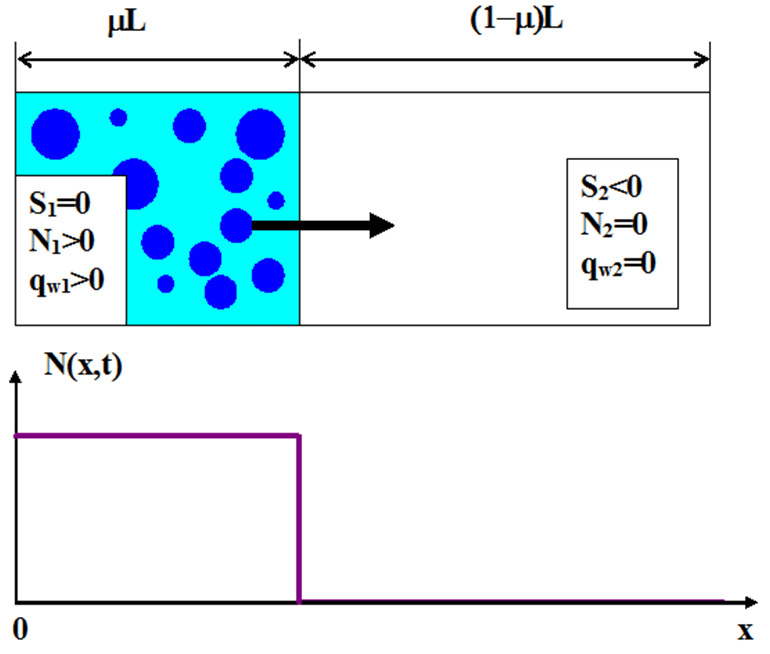
Figure 1The initial state at t=0. The left volume is a saturated cloudy volume; the right volume is an undersaturated dry air volume.
Like in Pt3, the process of turbulent diffusion is described by a 1-D equation of turbulent diffusion. The equation does not describe formation of separate turbulent filaments. Instead, it describes averaged effects of turbulent vortices of different scales by modeling of turbulent diffusion, characterized by a typical value of turbulent diffusion coefficient K. The mixing is assumed to be driven by isotropic turbulence at scales within the inertial sub-range where Richardson's law is valid. In this case, turbulent coefficient is evaluated as in Monin and Yaglom (1975):
In Eq. (1) ε is the turbulent kinetic energy dissipation rate and C=0.2 is a constant (Monin and Yaglom, 1975), Boffetta and Sokolov (2002). Equation (1) means that we consider the effects of turbulent diffusion at scales much larger than the Kolmogorov microscale; i.e., the effects of molecular diffusion are neglected. In the simulations, we use L=40 m and . This means that in the present study mixing is performed by vortices smaller than several tens of meters, which agrees with measurements in warm cumulus (Cu) (Gerber et al., 2008). The value of the turbulent kinetic energy dissipation rate chosen is also typical for small Cu (e.g., Gerber et al., 2008). These parameters correspond to Da values of several hundred. The model allows utilization of other values of L and ε typical of other cloud type (say, deep convective clouds), which can change results quantitatively, but not qualitatively.
Geometry of mixing and the initial conditions
The conceptual scheme presenting mixing geometry and the initial conditions used in the following analysis are shown in Fig. 1.
At t=0 the mixing volume of length L is divided into two volumes: the cloud volume of length μL and the dry volume of length (1−μ)L, where is the cloud volume fraction. The entire volume is assumed closed, i.e., adiabatic. At t=0 the cloud volume is assumed saturated, so the supersaturation S1=0. This volume is also characterized by the initial distribution of the square of the droplet radii g1(σ), where σ=r2. The initial liquid water mixing ratio in the cloudy volume is equal to . The integral of g1(σ) over σ is equal to the initial droplet concentration in the cloud volume . The initial droplet concentration in the dry volume is N2=0, the initial negative supersaturation in this volume is S2<0 and the initial liquid water mixing ratio qw2=0. Therefore, the initial profiles of these quantities along the x axis are step functions:
The initial profile of droplet concentration is shown in Fig. 1 (bottom). This is the simplest inhomogeneous mixing scheme, wherein mixing takes place only in the x direction, and the vertical velocity is neglected.
Since the total volume is adiabatic, the fluxes of different quantities through the left and right boundaries at any time instance are equal to zero, i.e.,
where qv is the water vapor mixing ratio.
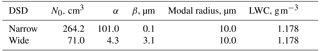
To investigate of mixing process for different initial DSD, we assume that DSD in the cloud volume can be represented by a gamma distribution:
where N0 is an intercept parameter, α is a shape parameter and β is a slope parameter of distribution. The DSD f(r) relates to distribution g1(σ) as f(r)=2rg1(σ). We performed simulations with both initially wide and narrow DSDs. The width of DSD is determined by a set of parameters. The parameters of the initial gamma distributions used in this study are presented in Table 1. Parameters of the distributions are chosen in such a way that the modal radii of DSD and the values of LWC are the same for both distributions. These distributions were used in Pt2 for analysis of homogeneous mixing.
Conservative quantity Γ(x,t)
The supersaturation equation for an adiabatic immovable volume can be written in the form , where S is supersaturation over water, and the coefficient is slightly dependent on temperature (Korolev and Mazin, 2003) (notations of other variables are presented in Appendix A). In our analysis we consider A2 to be a constant. As follows from the supersaturation equation, the quantity
is a conservative quantity, i.e., it is invariant with respect to phase transitions. In Eq. (5), |S(x,t)| can be comparable with unity by the order of magnitude. The conservative quantity Γ(x,t) obeys the following equation for turbulent diffusion,
with the adiabatic (no flux) condition at the left and right boundaries and the initial profile at t=0
From Eq. (7) it follows that Γ(x,0) is positive in the cloud volume and negative in the initially dry volume. The mean value of function Γ(x,0) can be written as follows:
can be either positive or negative. In the latter case a complete evaporation of droplets in the course of mixing takes place.
The solution of Eq. (6) with the initial condition Eq. (7) is (Polyanin et al., 2004):
One can see that function Γ(x,t) depends on three independent parameters A2qw1, S2 and μ. This function does not depend on the shape of the initial DSD in the cloud volume. In the final state when t→∞, Γ(x,t) is
Therefore, Γ(t=∞) depends on the cloud fraction and the initial values of the liquid water mixing ratio in the cloud volume and the relative humidity in the initially dry volume.
The final equilibrium values of supersaturation S(x,∞) and liquid water mixing ratio qw(x,∞) can be calculated using Eq. (5). The case corresponds to the equilibrium state with and , when droplets remain but do not evaporate any longer.
The case corresponds to the equilibrium state with and . In this equilibrium state droplets are totally evaporated, and volume remains subsaturated . At given qw1 and S2, there is a critical value of the cloud fraction μcr which separates these two possible final equilibrium states. This critical value corresponds to and can be calculated from Eq. (10) as
Another expression for μcr was formulated in Pt1.
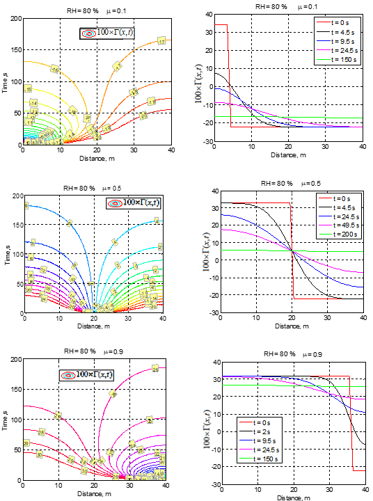
Figure 2Spatial–temporal variations of conservative function 100 × Γ(x,t) for different cloud fractions μ and initial RH2 = 80 %.
The examples of spatial–temporal variations of function Γ(x,t) for different cloud fractions and initial RH = 80 % are shown in Fig. 2.
The upper panels (μ=0.1) correspond to the case of final total droplet evaporation and negative final function Γ, whereas the middle and bottom rows (μ=0.5 and μ=0.9) illustrate partial evaporation cases when the total mixing volume reaches saturation. It is interesting that the time required for the final equilibrium state to be reached practically does not depend on the cloud fraction, which is ∼ 180 s for the illustrated cases. The cases μ=0.1 and μ=0.9 demonstrate a strong non-symmetric spatial variability of Γ(x) function during the first 50 s. At μ=0.5, a nearly full compensation between saturation deficit in the dry volume and available liquid water in the cloud volume takes place if at the equilibrium state. However, the compensation at μ=0.5 is not full because of the nonlinearity of Γ in Eq. (5).
Diffusion–evaporation equation for DSD
To formulate the diffusion–evaporation equation we use a simplified equation for droplet evaporation (Pruppacher and Klett, 1997), in which the curvature term and the chemical composition term are omitted
where (notations of other variables are presented in Appendix A).
The solution of Eq. (12) is
Equation (13) means that, in the course of evaporation, distribution g(σ) shifts to the left without changing its shape. The diffusion–evaporation equation for function can be written in the form
Combining Eqs. (12) and (14) yields
Equation (15) is similar to the diffusion–evaporation equation for size distribution function used in Pt3. The first term on the right-hand side of Eq. (15) describes the effect of turbulent diffusion, while the second term describes the changes of size distribution due to droplet evaporation. To close this equation, one can use Eq. (5) written as
and the equation for liquid water mixing ratio
The equation system (15–17) for distribution should be solved under the following initial condition,
and using the Neumann boundary conditions
These equations were solved numerically on a linear grid of droplet radii rj within the range 0–50 µm, where j=1…50 are the bin numbers. The number of grid points along the x axis was set equal to 81. In numerical calculations, the “evaporation term” in Eq. (15) was approximated as
A shift and subsequent remapping of DSD using the method proposed by Kovetz and Olund (1969) were implemented to solve Eq. (15) with the help of the MATLAB solver PDEPE. After calculation of the function, DSD was calculated using the relationship .
Mixing may take a significant time. Cloud microphysical parameters measured in in situ observations correspond to different stages of this transient mixing process. During mixing, DSDs and its parameters change substantially, which makes it reasonable to analyze these time changes.
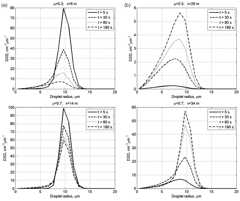
Figure 3Time evolution of DSD in the centers of the initially cloudy volume (a) and of the initially dry air volume (b) at initially narrow DSD. The initial mixing parameters are RH2 = 80 %, T = 10 ∘C, p = 828.8 mb and L = 40 m.
Figure 3 shows time evolution of initially narrow DSD in the centers of the cloudy volume and of the initially dry volume. The values of DSD in the initially cloudy volume decrease, while there are no significant changes in the DSD shape. At μ=0.7, the modal droplet radius remains unchanged during mixing staying equal to 10 µm. At μ=0.3, the effect of droplet diffusion on DSD is stronger, and mixing leads not only to a decrease in the DSD values but also to a decrease in the modal droplet radius in the cloudy volume. At both μ=0.3 and μ=0.7, mixing leads to broadening of the initial DSD due to the appearance of the tail of small droplets. The tail of small droplets is especially pronounced in the initially dry volume due to maximum evaporation of penetrated droplets.
The rate of the DSD growth in the initially dry volume depends on the value of the cloud fraction. At a low cloud fraction, the droplet concentration and droplet mass remain substantially lower for the main period of mixing process than that in the cloudy volume. At the same time, the modal DSD radius increases reaching 80 % of its maximum value already within the first 5 s. This is due to the fast increase in the relative humidity during mixing, so large droplets penetrating the initially dry volume do not decrease in size significantly determining only small changes of the values of modal, mean volume and effective radii. Thus, we see two stages of DSD evolution within the initially dry volumes: at the first stage penetrated droplets evaporate totally or partially. The partially evaporating droplets form the tail of small droplets. The formation of the tail of smallest droplets does not lead to significant changes in the size of the largest droplets. Note that according to the equation of diffusion growth/evaporation in sub-saturation conditions, the rate of droplet radii decreases inversely proportional to the droplet radius. This means that if, say, radius of a 2 µm droplet decreases twice during a certain time instance, the radius of a 20 µm droplet will decrease by less than 0.1 µm, i.e., remains approximately unchanged. At this stage, diffusion of water vapor from a cloudy volume and evaporation of penetrating droplets lead to a rapid growth of relative humidity RH. This growth of RH decreases evaporation rate of droplets penetrating initially dry volume later. At the second stage mixing leads to the increase in the droplet number due to droplet diffusion from cloudy volume. Since RH is high, this diffusion is not accompanied by significant change in droplet sizes, so DSD grows similarly at all radii.
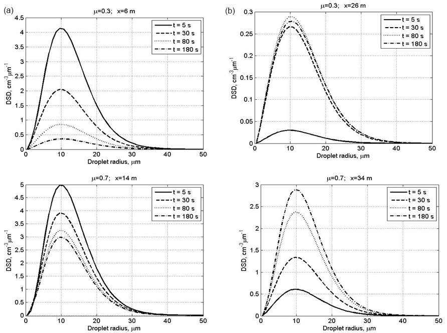
At the initially wide DSD (Fig. 4), the modal radii of the DSD do not change. This means that at the initial RH of 80 %, mixing and evaporation lead to a fast saturation of the initially dry volume, after which the peak radius remains unchanged in this volume. In the initially cloud volume RH remains close to 100 %, so the DSD decrease is related to dilution by initially dry air.
It is interesting that at μ=0.3, the maximum value of the DSD maximum in the initially dry volume is reached during the transition period (Fig. 4, at t = 80 s) and then decreases toward the equilibrium state. This behavior is caused by the competition between the diffusion and droplet evaporation.
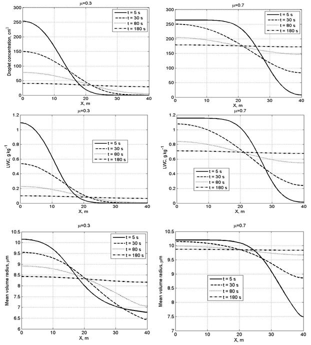
Figure 5Spatial dependences of droplet concentration, LWC and the mean volume radius within the mixing volume at different time instances at a narrow initial DSD. The initial mixing parameters are RH2 = 80 %, T = 10 ∘C, p = 828.8 mb and L = 40 m.
Figure 5 shows spatial dependences of droplet concentration, LWC and the mean volume radius within the mixing volume at different time instances at narrow initial DSD. At small values of the cloud fraction, diffusion of water vapor and droplets, as well as droplet evaporation, leads to a fast decrease in droplet concentration and LWC in the initially cloud volume. The mean volume radius in this volume decreases by about 15 % in the course of mixing. It is natural that, at a large cloud fraction, droplet concentration and LWC in the initially cloudy volume decrease slowly, while these quantities in the initially dry volume increase rapidly. At both small and large cloud fractions, the mean volume radius in the initially dry volume grows rapidly during the mixing toward its values in the initially cloudy volumes, even if droplet concentration and LWC remain much lower than in the adjacent cloud volume.
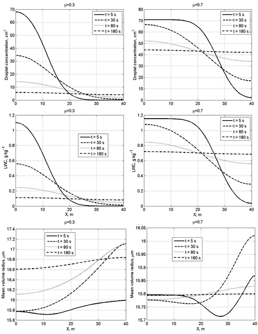
Figure 6 shows the spatial dependences of droplet concentration, LWC and the mean volume radius within the mixing volume at different time instances at wide initial DSD.
A specific feature of mixing at a wide DSD is the increase in the mean volume radius, so the ratio . In the course of mixing, the mean volume radius maximum is reached in the initially dry volumes. This result can be attributed to the fact that in this volume smaller droplets fully evaporate, so the concentration of large droplets increases with respect to concentration of smaller droplets (Fig. 4, right column). Scattering diagrams plotted using in situ observations often contain points or groups of points with (or , where re is effective radius) within a wide range of normalized droplet concentration (e.g., Burnet and Brenguier, 2007; Krueger et al., 2006; Gerber et al., 2008). The result obtained in the present study shows that the behavior of with time in the course of mixing may depend on the DSD shape in the initially cloud volume that determines the ratio between concentrations of small and large droplets in the course of mixing. Of course, the DSD shape is only one possible reason for the appearance of points with on the scattering diagram.
We see that the transition to the final equilibrium state within the volume with the spatial scale of 40 m is about 5 min (Fig. 7), which is a comparatively long period of time compared to the characteristic times of other microphysical processes, including droplet evaporation. During this time the DSD changes substantially, especially at small cloud fraction. The mean volume radius in the initially dry volume increases much faster than LWC. As a result, mean volume radius in such a volume rapidly reaches the values typical of cloudy air, while LWC still remains substantially lower than in the cloudy volume. Despite some DSD broadening, the final DSDs in the mixing volume resemble those in the initially cloud volumes. The main effect of mixing is lowering the DSD values as the cloud fraction decreases.
This study reconsiders the classical theory of mixing diagrams. In the classical theory two volumes (cloudy and droplet-free) mix with each other within a given unmovable mixing volume (see review by Korolev et al., 2016). Mixing diagrams are typically plotted for times when all variables become uniform within the mixing volume, i.e., when the equilibrium state is reached. We plot the mixing diagram using the same simplifications used in the plotting classical mixing diagrams, namely no vertical motions and no collisions are assumed. These assumptions allow for better revealing the microphysical effects of turbulent mixing. It is widely assumed that the mixing type is determined by the Damköhler number, which depends only on drop relaxation time and mixing time. No averaged vertical velocity and no collision rate are included into this criterion.
We extend the theory, however, in several important aspects concerning microphysical effects: (a) we consider the time-dependent process of mixing and (b) initial droplet size distributions are assumed polydisperse.
Mixing considered in the present study always leads to the equilibrium state. As was explained above, two equilibrium states are possible. The first one is characterized by the total evaporation of cloud droplets , whereas the second one occurs if the air in the mixing volume becomes saturated, i.e., when . At the given initial values of qw1 in the cloud volume and of S2 in the initially dry volume, there always exists the cloud fraction μcr (Eq. 11) separating these two states.
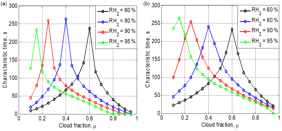
Figure 7Time required to reach the equilibrium state vs. the cloud fraction at different initial RH for the initially narrow DSD (a) and the initially wide DSD (b). Parameters of DSD are given in Table 1. The initial mixing parameters are T = 10 ∘C, p = 828.8 mb and L = 40 m.
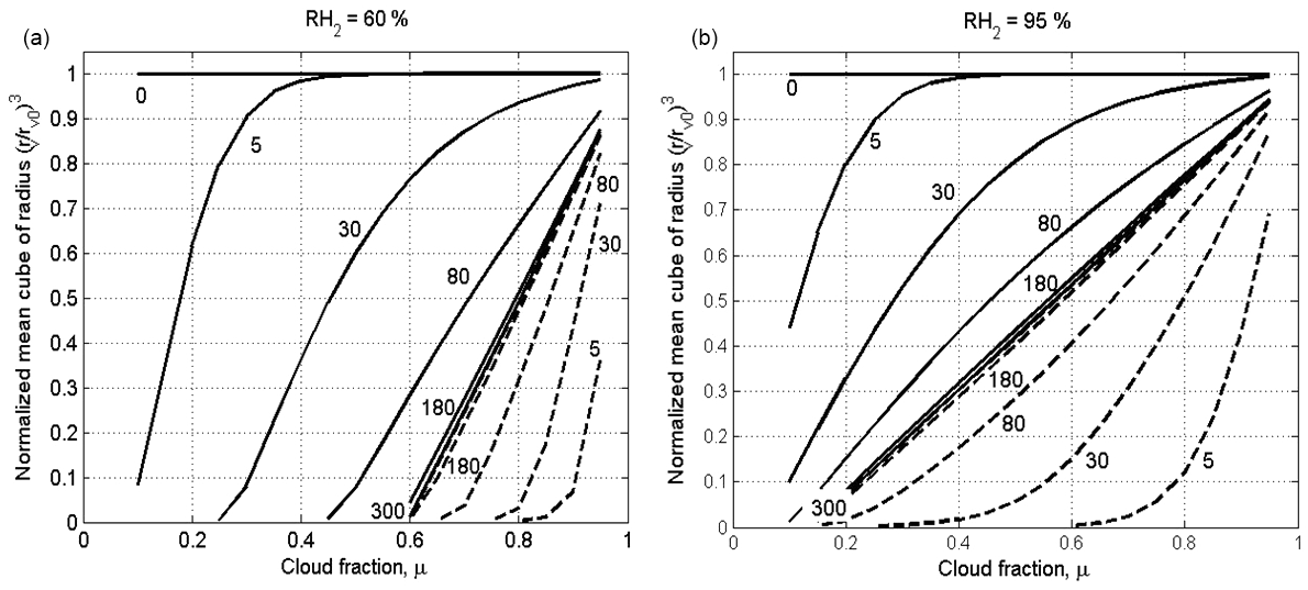
Figure 8Dependences of the normalized cube of the mean volume radius on the cloud fraction at different time instances for x=0 (solid lines) corresponding to the initially cloud volume, and x=L (dash line) corresponding to the initially dry volume. The time instances in seconds are marked by numbers. The figure is plotted for the narrow initial DSD for two values of RH2: 60 % (a) and 95 % (b). Parameters of DSD are given in Table 1. The initial mixing parameters are T = 10 ∘C, p = 828.8 mb and L = 40 m. Calculations performed within the range of .
4.1 The process of achieving the equilibrium state
Figure 7 shows the dependences of the time required to reach the equilibrium on the cloud fraction, at different initial relative humidity values in the dry volume and two initial DSDs (the parameters are presented in Table 1). The characteristic time is defined here as the time from the beginning of mixing to the time instance when inequality becomes valid. The mean droplet concentration is calculated by averaging along x axes (. In the case of a total evaporation, .
Each curve in Fig. 7 consists of two branches. The left branches correspond to the total evaporation regime, while the right branches correspond to the partial evaporation at equilibrium. The maximum time corresponds to the situation when the available amount of liquid water is approximately equal to the saturation deficit. A similar result was obtained in Pt1 and Pt2 for homogeneous mixing. The maximum values of the characteristic time are about 4 min for a mixing volume of 40 m in length. The right branches show that the characteristic time decreases with increasing cloud fraction. Despite some differences in the curve slopes, the characteristic times for wide and narrow DSD are quite similar.
Figure 8 shows dependences of the normalized cube of the mean volume radius on the cloud fraction at different time instances for two values of x: x=0 (solid lines) corresponds to the initially cloudy volume, and x=L (dashed line) corresponds to the initially dry volume. The figure is plotted for the narrow DSD for two values of RH2: 60 and 95 %. Despite the fact that the diffusion–evaporation equation allows simulating using any initial RH, we do not consider in our examples the cases of very low RH of dry volume. This is because at very low RH, say RH = 20 %, the cloud fraction should exceed 0.8 to prevent total droplet evaporation in the equilibrium state (at LWC = 1 g kg−1). At the same time, we are interested in the equilibrium state at which droplets exist. Note that at the lateral edges of warm Cu a shell of humid air arises, so RH of the entrained air should be high enough (e.g., Gerber et al., 2008).
The curve plotted for the time instance of 300 s corresponds to the equilibrium state (hereafter the equilibrium curve). The curves above the equilibrium curve correspond to the initially cloudy volume, and the curves below the equilibrium curve correspond to the initially dry volume. One can see how curves of both types approach the same final state. During the mixing the curves move over the plane toward the equilibrium curve. As a result, the curves plotted in Fig. 8, corresponding to different time instances of the mixing, together cover the entire area of the panels.
During this movement the distance from the curves to the horizontal line changes, and the curves' slopes increase. In our case of L = 40 m, the mixing remains inhomogeneous the during entire mixing process, so the change in the distance from the curves to the horizontal line characterizes the temporal changes over the mixing process, but not a change in mixing type.
It is noteworthy in this relation that scattering diagrams plotted using in situ observations reflect mixing between different multiple volumes at different stages of the mixing process. Accordingly, points in the scattering diagrams can be far from the equilibrium location. Figure 8 indicates, therefore, that scattering diagrams show snapshots of transient mixing process when the distance from points in the diagrams to line characterizes the stage of the mixing process, but not the mixing type.
The dependences of the normalized cube of the mean volume radius on the cloud fraction at different time instances at wide DSD also indicate approaching to the equilibrium curve, while all the curves correspond to (not shown).
Note that in several studies normalized effective radius is used for plotting scattering and mixing diagrams, but not mean volume radius (Gerber et al., 2008; Freud et al., 2011). Comparison of scattering and mixing diagrams in the study plotted using mean volume and effective radii did not reveal any significant differences (not shown).
4.2 Mixing diagrams
Using the diffusion–evaporation equations (Eqs. 15–17) we calculated the equilibrium DSD for different initial relative humidity values and different cloud fractions. Each calculation was performed for both narrow and wide initial DSD (parameters shown in Table 1). These equilibrium DSDs were used to calculate mixing diagrams showing dependences of the normalized cube of the effective radius on the cloud fraction.

Figure 9Mixing diagrams. Normalized cube of the mean volume radius vs. the cloud fraction for initial narrow DSD (a) and initial wide DSD (b). The dependencies correspond to the equilibrium state. Parameters of initial DSD are presented in Table 1. Solid and dashed lines show the mixing diagrams for inhomogeneous and homogeneous mixing, respectively. The initial mixing parameters are T = 10 ∘C, p = 828.8 mb and L = 40 m.
The corresponding mixing diagrams for homogeneous mixing case were also calculated for comparison. To this effect, the supersaturation and DSD in both the cloud and the dry volumes were aligned, taking into account the cloud fraction value μ. The alignment led to the following initial values of supersaturation and DSD within the mixing volume:
Upon the alignment, time evolution values of DSD under homogeneous evaporation in an adiabatic immovable parcel were calculated until the equilibrium state was reached. These equilibrium DSDs were used to calculate mixing diagrams for homogeneous mixing. To do this, we used the parcel model proposed by Korolev (1995) that describes evaporation by means of equations with temperature-dependent parameters. Figure 9 shows the mixing diagrams plotted for initial narrow and wide DSD cases.
While all the curves in the mixing diagram for narrow DSD are below the straight line , the curves for wide DSD are above this line. The explanation of this effect is given in Sect. 3 (Fig. 6). The curves plotted for homogeneous and inhomogeneous mixing demonstrate an important feature, namely that, at given values of RH and qw1 in the initially dry volume, the values μcr of the cloud fraction at which all the droplets evaporate are approximately the same for any type of mixing. This condition is the consequence of the mass conservation law determined by Eq. (11) and does not depend on the initial DSD shape. In standard mixing diagrams (e.g., Lehmann et al., 2009; Gerber et al., 2008; Freud et al., 2011), the horizontal straight line (or is typically plotted for the entire range of the cloud fraction [0…1], while the curves corresponding to homogeneous mixing are plotted for different RH within the range [μcr(RH2)…1]. As a result, the high difference between extremely inhomogeneous and homogeneous mixing types is clearly seen at low RH and at small cloud fractions. The condition that μcr is the same for different mixing types indicates that the mixing diagrams may look nearly similar for μ>μcr. This means that the range of the cloud fractions required for comparison of diagrams aimed at determination of a mixing type shortens as RH2 values in the surrounding air decrease.
The comparison of panels (a) and (b) in Fig. 9 shows that the differences between the diagrams for homogeneous and inhomogeneous mixing types are more pronounced for initially narrow DSD. The maximum difference should take place for monodisperse DSD considered in Pt1, Pt2 and Pt3. Within the range of μ>μcr, the distance between the curves corresponding to different mixing regimes is small even for narrow DSD and low RH2. The lower difference is related to the fact that at high RH2 the curves in the mixing diagrams are close to the horizontal straight line in both regimes, while at low RH2, μcr is small and both curves should drop to zero in the vicinity of μ=μcr.
As regards the wide DSD case, the difference between the curves corresponding to different mixing type is negligible (Fig. 9b)
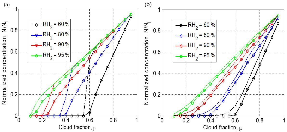
Figure 10Final normalized droplet concentration vs. cloud fraction for initially narrow DSD (a) and initially wide DSD (b). Parameters of initial DSD are shown in Table 1. Dashed line shows the results of equivalent homogeneous mixing. The initial mixing parameters are T = 10 ∘C, p = 828.8 mb and L = 40 m.

Figure 11Dependencies of the normalized cube of the mean volume radius on normalized droplet concentration for different initial relative humidity values. (a) Narrow initial DSD. (b) Wide initial DSD. The initial mixing parameters are T = 10 ∘C, p = 828.8 mb and L = 40 m.
4.3 Effect of the relative humidity
In measurements carried out at cloud boundaries and in cloud simulations, the cloud fraction is not known; therefore, it is widely accepted to use normalized droplet concentration instead of the cloud fraction (Burnet and Brenguier, 2007; Gerber et al., 2008: Lehmann et al., 2009). Droplet concentration is normalized by the maximum value along the airplane traverse. The difference between the cloud fraction and normalized droplet concentration is obvious: the cloud fraction is a parameter given as the initial condition. At the same time, normalized droplet concentration changes with time and space due to complete evaporation of some droplet fraction. Figure 10 shows dependencies of normalized droplet concentration on the cloud fraction at the equilibrium final state of mixing. One can see a substantial deviation from 1:1 linear dependence, especially at low RH. Note that droplet concentration decreases in the course of both homogeneous and inhomogeneous mixing if the initial DSDs are polydisperse. The fraction of totally evaporating droplets increases with decreasing RH2. As expected, droplet concentration in homogeneous mixing is higher than that in inhomogeneous mixing. The difference between droplet concentrations at wide DSD is lower than at narrow DSD.
Figure 11 shows the dependencies on normalized droplet concentration for narrow and wide DSD in inhomogeneous mixing. The normalization by droplet concentration in the initially cloud volume at t=0 was used. Taking into account the dependences of normalized droplet concentration on the cloud fraction μ (Fig. 10), one can get the curves shown in Fig. 11 which actually coincide at different RH2. The lack of the sensitivity to RH2 can be attributed to the fact that a decrease in RH leads to a decrease in normalized droplet concentration, so the curves corresponding to low RH in Fig. 9 shift to the left when the normalized droplet concentration is used instead of μ. The shape of the dependences in Fig. 11b is explained by an increase in the mean volume radius with decreasing droplet concentration.
Thus, the mixing diagrams plotted in the plane vs. normalized droplet concentration do not depend on the relative humidity of the surrounding dry air. This result indicates an additional difficulty in distinguishing between mixing types based on scattering diagrams plotted using in situ data in these axes. The concentration of observed points in these scattering diagrams close to the line is often interpreted as an indication of homogeneous mixing, but at high RH in the surrounding air (Gerber et al., 2008; Lehmann et al., 2009). High values of RH in the penetrating air volumes are usually explained by formation of a layer of moist air around the cloud boundary (Gerber et al., 2008; Knight and Miller, 1998).
The reference values of droplet concentration and the effective radius used for normalization in the present study are taken as the initial values in the cloud volume before it mixes with the neighboring dry volume. In real in situ measurements the reference values of these quantities are typically chosen in a less diluted cloud volume along the airplane traverse. This reference volume may be quite remote from the particular mixing volume. It can lead to a shift of the mixing diagram with respect to the line, as well as to a large variation in mixing diagram shapes, which are not related, however, to the mixing type (e.g., Lehmann et al., 2009).
This study extends the analysis of mixing performed in Pt3, where the diffusion–evaporation equation served as the basis, the initial DSD were assumed monodisperse and the cloud fraction was chosen as . In the present study, the analysis focuses on the temporal and spatial evolution of initially polydisperse DSD and investigates mixing diagrams obtained for narrow and wide initial DSD within a wide range of the cloud fraction values (0.1–0.95). It is shown that results of mixing and the structure of mixing diagrams depend on the initial DSD shape. This finding indicates that mixing is a problem that cannot be determined by a single parameter (e.g., the Damkölher number as often assumed) or even by two parameters (the Damkölher number and the potential evaporation parameters as assumed in Pt3). The temporal changes of DSD and their moments during mixing are calculated. Although DSD broaden, they tend to remain similar to the original DSD. The main changes come from the cloud air dilution by the dry air, which leads to a decrease in droplet concentration for all droplet sizes. The changes of DSD and its shape are minimum in the initially cloud volumes, especially at significant cloud fractions. The droplet radii corresponding to the DSD peak do not change significantly in any case. In the initially dry volumes, mixing and evaporation of penetrated droplets leads to a rapid increase in RH. Consequently, large droplets penetrating these volumes do not change their sizes significantly. As a result, the mean volume radius in these volumes rapidly increases and reaches the values typical of cloud volumes, while LWC remains lower than in the cloud volume for most of the mixing time. At narrow DSD, the mean volume (and effective) radius remains smaller than that in the initially cloud volume. At wide DSD, the mean volume (and effective) radius may become larger than that in the initial DSD. This increase in the effective radius is attributed to the fact that evaporation of smaller droplets leads to the increase in the fraction of larger droplets in the DSD. In this study, and in Pt3, it is shown that mixing leads to DSD broadening. This contrasts with the classical theory, in which initially monodisperse DSDs remain monodisperse in the course of mixing. This problem is analyzed in detail in Pt 3. Note that in real clouds there are many mechanisms leading to DSDs broadening (e.g., Pinsky and Khain, 2002).
Dependences of the normalized cube of the mean volume radius on the cloud fraction (rv∕rv0)3 as a function of μ at different time instances form the set of curves filling the entire plane. Therefore, both the slope and the distance of these curves with respect to the horizontal line change with time. This means that this distance characterizes the temporal changes in the course of mixing, but not the mixing type (which remains inhomogeneous during the entire mixing time). The mixing process is comparatively long (several minutes), so the final equilibrium stage is hardly achievable in real clouds.
It is highly important that the critical values of the cloud fraction μcr corresponding to total droplet evaporation are the same for any mixing type. This means that the curves in a mixing diagram corresponding to homogeneous and inhomogeneous mixing types should be compared only within the range of μ>μcr. The range width of μ>μcr decreases with decreasing relative humidity in the initially dry volume. Taking into account significant scattering of observed points, this condition greatly hampers the problem of how to distinguish between mixing types.
Another important result of the study is that mixing diagrams for homogeneous and inhomogeneous mixing plotted for polydisperse DSD do not differ much. The largest difference occurs for initially narrow DSD (the maximum difference takes place for initially monodisperse DSD), but even in this case the difference is not large enough to reliably distinguish mixing type, owing to the significant scatter of observed data. At wide DSD, this difference between mixing diagrams for homogeneous and inhomogeneous becomes negligibly small.
The cloud fraction μ is a predefined parameter and is not determined from observations. Consequently, in the analysis of in situ measurements the normalized droplet concentration is typically used instead of the cloud fraction. However, there is a significant difference between the cloud fraction prescribed a priori and the normalized droplet concentration that changes due to total evaporation of some fraction of droplets. We have shown that the utilization of normalized droplet concentration in mixing diagrams is not equivalent to the utilization of the cloud fraction. The important conclusion is that when mixing diagrams are plotted using the normalized concentration, the sensitivity to RH disappears. This conclusion is valid even when RH in the initially dry volume is as low as 60 %. This conclusion clearly contradicts the widespread assumption that mixing types can be easily distinguished in mixing diagrams in case of low relative humidity of the surrounding air.
In the present study as well as in Pt3 and modeling studies performed by Andrejczuk et al. (2006, 2009) and Khain et al. (2018), it is shown that time needed to establish equilibrium is either quite long or even never reached. This means that the scattering diagrams observed in situ are just snapshots of the transient mixing process. In order to show how different the equilibrium and intermediate states are, we investigate the transition to such equilibrium assuming that the mixing volume remains adiabatic (i.e., isolated) during the entire period of mixing. This is, of course, a serious simplification made to compare the results with those predicted by the classical concept. Another simplification of the model is the neglecting the intermittency in the process of mixing that takes place in real clouds.
To summarize, our general conclusion is that the simplifications underlying the classical concept of mixing are too crude, making it impossible to use scattering diagrams for comprehensive analysis of mixing and especially for determination of mixing types. At the same time, scattering diagrams may contain useful information concerning intensity of mixing, the DSD width and other parameters of DSDs (see Khain et al., 2018).
| Symbol | Description | Units |
|---|---|---|
| A2 | , coefficient | – |
| an | Fourier series coefficients | – |
| C | Richardson's law constant | – |
| cp | specific heat capacity of moist air at constant pressure | |
| D | coefficient of water vapor diffusion in air | m2 s−1 |
| Da | Damkölher number | – |
| e | water vapor pressure | N m−2 |
| ew | saturation vapor pressure above flat surface of water | N m−2 |
| F | , coefficient | m−2 s |
| f(r) | droplet size distribution | m−4 |
| g(r) | droplet size distribution | m−5 |
| g0(σ) | initial distribution of square radius in homogeneous mixing | m−5 |
| g1(σ) | initial distribution of square radius | m−5 |
| ka | coefficient of air heat conductivity | |
| K | turbulent diffusion coefficient | m2 s−1 |
| L | characteristic spatial scale of mixing | m |
| Lw | latent heat for liquid water | J kg−1 |
| N | droplet concentration | m−3 |
| N0 | parameter of gamma distribution | m−3 |
| mean droplet concentration | m−3 | |
| N1 | initial droplet concentration in cloud volume | m−3 |
| p | pressure of moist air | N m−2 |
| qv | water vapor mixing ratio (mass of water vapor per 1 kg of dry air) | – |
| qw | liquid water mixing ratio (mass of liquid water per 1 kg of dry air) | – |
| qw1 | liquid water mixing ratio in cloud volume | – |
| R | , non-dimensional parameter | – |
| Rv | specific gas constant of water vapor | |
| r | droplet radius | m |
| r1 | initial droplet radius | m |
| re | effective radius | m |
| re0 | initial effective radius | m |
| S | supersaturation over water | – |
| S2 | initial supersaturation in the dry volume | – |
| S0 | initial supersaturation in homogeneous mixing | – |
| T | temperature | K |
| t | time | s |
| x | distance | m |
| α | parameter of gamma distribution | – |
| β | parameter of gamma distribution | m−1 |
| Δt | time step | s |
| μ | cloud fraction | – |
| μcr | critical cloud fraction | – |
| ε | turbulent dissipation rate | m2 s−3 |
| Γ(x,t) | conservative function | – |
| ρa | air density | kg m−3 |
| ρw | liquid water density | kg m−3 |
| σ | square of droplet radius | m2 |
Codes of the diffusional–evaporation model are available upon request.
The authors declare that they have no conflict of interest.
This research was supported by the Israel Science Foundation (grants 1393/14,
2027/17) and the Office of Science (BER) of the US Department of Energy
(award DE-SC0006788, DE-FOA-0001638).
Edited by:
Timothy Garrett
Reviewed by: two anonymous referees
Andrejczuk, M., Grabowski, W. W., Malinowski, S. P., and Smolarkiewicz, P. K.: Numerical simulation of cloud–clear air interfacial mixing: effects on cloud microphysics, J. Atmos. Sci., 63, 3204–3225, 2006.
Andrejczuk, M., Grabowski, W. W., Malinowski, S. P., and Smolarkiewicz, P. K.: Numerical simulation of cloud–clear air interfacial mixing: homogeneous versus inhomogeneous mixing, J. Atmos. Sci., 66, 2493–2500, https://doi.org/10.1175/2009JAS2956.1, 2009.
Bera, S., Prabha, T. V., and Grabowski, W. W.: Observations of monsoon convective cloud microphysics over India and role of entrainment-mixing, J. Geophys. Res.-Atmos., 121, 9767–9788, https://doi.org/10.1002/2016JD025133, 2016a.
Bera, S., Pandithurai, G., and Prabha, T. V.: Entrainment and droplet spectral characteristics in convective clouds during transition to monsoon, Atmos. Sci. Lett., 17, 286–293, 2016b.
Boffetta, G. and Sokolov, I. M.: Relative dispersion in fully developed turbulence: the Richardson's Law and intermittency correction, Phys. Rev. Lett., 88, 094501, https://doi.org/10.1103/PhysRevLett.88.094501, 2002.
Burnet, F. and Brenguier, J.-L: Observational study of the entrainment-mixing process in warm convective cloud, J. Atmos. Sci., 64, 1995–2011, 2007.
Devenish, B. J., Bartello, P., Brenguier, J.-L., Collins, L. R., Grabowski, W. W., Ijzermans, R. H. A., Malinovski, S. P., Reeks, M. W., Vassilicos, J. C., Wang, L.-P., and Warhaft, Z.: Droplet growth in warm turbulent clouds, Q. J. Roy. Meteor. Soc., 138, 1401–1429, 2012.
Freud, E., Rosenfeld, D., and Kulkarni, J. R.: Resolving both entrainment-mixing and number of activated CCN in deep convective clouds, Atmos. Chem. Phys., 11, 12887–12900, https://doi.org/10.5194/acp-11-12887-2011, 2011.
Gerber, H., Frick, G., Jensen, J.B., and Hudson, J. G.: Entrainment, mixing, and microphysics in trade-wind cumulus, J. Meteorol. Soc. Jpn., 86A, 87–106, 2008.
Khain, A. P., Ovchinnikov, M., Pinsky, M., Pokrovsky, A., and Krugliak, H.: Notes on the state-of-the-art numerical modeling of cloud microphysics, Atmos. Res., 55, 159–224, 2000.
Khain, A., Prabha, T. V., Benmoshe, N., Pandithurai, G., and Ovchinnikov, M.: The mechanism of first raindrops formation in deep convective clouds, J. Geophys. Res.-Atmos., 118, 9123–9140, 2013.
Khain, A., Pinsky, M., and Magaritz-Ronen, L.: Physical interpretation of mixing diagrams, J. Geophys. Res.-Atmos., 123, 529–542, 2018.
Knight, C. A. and Miller, L. J.: Early radar echoes from small, warm cumulus: Bragg and hydrometeor scattering, J. Atmos. Sci., 55, 2974–2992, 1998.
Korolev, A. V.: The influence of supersaturation fluctuations on droplet size spectra formation, J. Atmos. Sci., 52, 3620–3634, 1995.
Korolev, A. and Mazin, I.: Supersaturation of water vapor in clouds, J. Atmos. Sci., 60, 2957–2974, 2003.
Korolev, A., Khain, A., Pinsky, M., and French, J.: Theoretical study of mixing in liquid clouds – Part 1: Classical concepts, Atmos. Chem. Phys., 16, 9235–9254, https://doi.org/10.5194/acp-16-9235-2016, 2016.
Kovetz, A. and Olund, B.: The effect of coalescence and condensation on rain formation in a cloud of finite vertical extent, J. Atmos. Sci., 26, 1060–1065, 1969.
Krueger, S. K., Lehr, P. J., and Su, C. W.: How entrainment and mixing scenarios affect droplet spectra in cumulus clouds, in: 12th Conference on Cloud Physics, and 12th Conference on Atmospheric Radiation, Madison, WI, 2006.
Kumar, B., Schumacher, J., and Shaw, R. A.: Lagrangian mixing dynamics at the cloudy–clear air interface, J. Atmos. Sci., 71, 2564–2579, 2014.
Kumar, B., Bera, S., Prabha, T. V., and Grabowski, W. W.: Cloud-edge mixing: direct numerical simulation and observations in Indian Monsoon clouds, J. Adv. Model. Earth Sy., 9, 332–353, https://doi.org/10.1002/2016MS000731, 2017.
Lehmann, K., Siebert, H., and Shaw, R. A.: Homogeneous and inhomogeneous mixing in cumulus clouds: dependence on local turbulence structure, J. Atmos. Sci., 66, 3641–3659, 2009.
Magaritz-Ronen, L., Pinsky, M., and Khain, A.: Drizzle formation in stratocumulus clouds: effects of turbulent mixing, Atmos. Chem. Phys., 16, 1849–1862, https://doi.org/10.5194/acp-16-1849-2016, 2016.
Monin, A. S. and Yaglom, A. M.: Statistical Fluid Mechanics: Mechanics of Turbulence, vol. 2, MIT Press, Boston, USA, 1975.
Pinsky, M. and Khain, A. P.: Effects of in-cloud nucleation and turbulence on droplet spectrum formation in cumulus clouds, Q. J. Roy. Meteor. Soc., 128, 1–33, 2002.
Pinsky, M., Khain, A., Korolev, A., and Magaritz-Ronen, L.: Theoretical investigation of mixing in warm clouds – Part 2: Homogeneous mixing, Atmos. Chem. Phys., 16, 9255-9272, https://doi.org/10.5194/acp-16-9255-2016, 2016a.
Pinsky, M., Khain, A., and Korolev, A.: Theoretical analysis of mixing in liquid clouds – Part 3: Inhomogeneous mixing, Atmos. Chem. Phys., 16, 9273-9297, https://doi.org/10.5194/acp-16-9273-2016, 2016b.
Polyanin, A. D. and Zaitsev, V. F.: Handbook of Nonlinear Partial Differential Equations, Chapman & Hall/CRC, 809 pp., 2004.
Prabha, T., Khain, A. P., Goswami, B. N., Pandithurai, G., Maheshkumar, R. S., and Kulkarni, J. R.: Microphysics of pre-monsoon and monsoon clouds as seen from in-situ measurements during CAIPEEX, J. Atmos. Sci., 68, 1882–1901, 2011.
Pruppacher, H. R. and Klett, J. D.: Microphysics of Clouds and Precipitation, 2nd edn., Oxford Press, Boston, London, 914 p., 1997.
Segal, Y., Khain, A. P., and Pinsky, M.: Theromodynamic factors influencing the bimodal spectra formation in cumulus clouds, Atmos. Res., 66, 43–64, 2003.
Yang, F., Shaw, R., and Xue, H.: Conditions for super-adiabatic droplet growth after entrainment mixing, Atmos. Chem. Phys., 16, 9421–9433, https://doi.org/10.5194/acp-16-9421-2016, 2016.
Yum, S. S., Wang, J., Liu, Y., Senum, G., Springston, S., McGraw, R., and Yeom, J. M.: Cloud microphysical relationships and their implication on entrainment and mixing mechanism for the stratocumulus clouds measured during the VOCALS project, J. Geophys. Res., 120, 5047–5069, https://doi.org/10.1002/2014JD022802, 2015.
- Article
(10194 KB) - Full-text XML