Different trends in extreme and median surface aerosol extinction coefficients over China inferred from quality-controlled visibility data

Although the temporal changes in aerosol properties have been widely investigated, the majority of studies has focused on average conditions without much emphasis on the extremes. However, the latter can be more important in terms of human health and climate change. This study uses a previously validated, quality-controlled visibility dataset to investigate the long-term trends (expressed in terms of relative changes) in extreme surface aerosol extinction coefficient (AEC) over China and compares them with the median trends. Two methods are used to independently evaluate the trends, which arrive at consistent results. The signs of extreme and median trends are generally coherent, whereas their magnitudes show distinct spatial and temporal differences. In the 1980s, an overall positive trend is found throughout China with the extreme trend exceeding the mean trend, except for northwest China and the North China Plain. In the 1990s, AEC over northeast and northwest China started to decline while the rest of the country still exhibited an increase. The extreme trends continued to dominate in the south while they yielded to the mean trend in the north. After the year 2000, the extreme trend became weaker than the mean trend overall in terms of both the magnitude and significance level. The annual trend can be primarily attributed to winter and fall trends. The results suggest that the decadal changes in pollution in China may be governed by different mechanisms. Synoptic conditions that often result in extreme air quality changes might have dominated in the 1980s, whereas emission increase might have been the main factor for the 2000s.

1 Introduction

As a by-product of rapid industrial and economic development, China has been faced with a serious issue of air pollution. The variability and trends in China's air quality or aerosol properties have become the focus of numerous past studies (Jinhuan and Liquan, 2000; Che et al., 2007; Deng et al., 2008; Streets et al., 2008; Yoon et al., 2011; Guo et al., 2011; Zhang et al., 2015). While many of these works reached important conclusions about the temporal evolution of China's pollution, the majority only analyzed the arithmetic means (e.g., monthly or annual means of aerosol optical depth), with little attention paid to the extreme values. However, it is often these extremes that are responsible for many health- and climate-related consequences. Additionally, considering that the distribution of aerosol optical properties, such as aerosol optical depth (AOD) and extinction coefficients, is often highly right-skewed (O'Neill et al., 2000; Collaud Coen et al., 2013; Yoon et al., 2016), analyzing the arithmetic mean tends to discard the large portion of information in the long tails, thus biasing the result. Moreover, as indicated by previous studies, extreme pollution events are often associated with abnormal synoptic conditions (Zheng et al., 2015; Ye et al., 2016), whereas the mean should be more prone to changes in the emission, which increases pollution level overall. Therefore, analyzing the changes in both the mean and extreme values would help understand the factors influencing the variability in pollution.

For the few studies that have addressed temporal changes in the percentiles of aerosol loading, usually either satellite- or surface-based remote-sensing measurements are used, such as AOD retrievals from the Moderate Resolution Imaging Spectroradiometer (MODIS; Sullivan et al., 2015) or the Aerosol Robotic Network (AERONET; Xia, 2011; Yoon et al., 2016). Nonetheless, remote-sensing data are not ideal for extreme analysis, mainly because they frequently miss heavy pollution conditions likely associated with strict cloud screening (Lin and Li, 2016). Moreover, remote-sensing techniques cannot recognize mixed-layer height, a major parameter affecting surface air pollution, which hinders their use for air quality studies. As a result, the “real” extremely high aerosol loadings cannot be well detected using remote sensing. On the other hand, surface visibility observations that do not require cloud screening or other retrieval assumptions can serve as a suitable alternative for pollution-related research. After eliminating fog, rain or snow conditions, the degradation of surface visibility can be mainly attributed to aerosol extinction and is thus closely related to air quality (Husar et al., 2000). Moreover, since routine visibility observation started as early as the 1970s for many sites, these data can offer a much longer time series for trend analysis than remote-sensing products. Previously, Li et al. (2016) used a quality-controlled (by comparing against surface PM₁₀ and PM_2.5 measurements) visibility-converted aerosol extinction coefficient (AEC) dataset to study temporal changes in monthly mean surface aerosol extinction in China for the past 30 years and found that there are obvious shifts in the trends for different time periods. However, it still remains to be understood whether the extreme values change faster or slower than the mean.

In this paper, we use the same dataset as in Li et al. (2016) to further investigate the trends in extremely high (defined as the 95th percentile) surface aerosol extinction coefficients and compare them with the median trends representing average conditions. Although a threshold visibility value is often used in previous studies to define extreme events (for example, Fu et al., 2013, define extreme pollution as visibility lower than 5 km), the same threshold does not apply to all sites since their reporting conventions may be different. We thus believe a percentile criterion would be more appropriate. In addition to estimating the linear trend in the 95th percentile value itself, we also use a novel method proposed by Franzke (2013) based on quantile regression with surrogate data testing for significance. Franzke (2013) used this method to test for significant trends in extreme temperatures. To our knowledge, this method has not been applied to aerosol-related research, and the independent application of two methods increases the robustness of the results.

In Sect. 2, we describe the data and method used in this study. The analysis results are presented in Sect. 3, followed by the conclusions and a brief discussion in Sect. 4.

2 Data and methods

2.1 Visibility data

Here we use the same visibility dataset as in Li et al. (2016). This hourly surface visibility dataset is obtained from the National Centers for Environmental Information (NCDC; http://www1.ncdc.noaa.gov/pub/data/noaa/) of the National Oceanic and Atmospheric Administration (NOAA). The data selection criteria and quality control procedure strictly follows those implemented by Li et al. (2016). Briefly, data before 1980 are not used because of a different reporting standard (Che et al., 2007; Wu et al., 2012). Those after 2013 are also excluded because many sites have replaced human observation with automatic visibility sensors. Then the eight quality assurance steps proposed by Li et al. (2016) are applied to the dataset. A total of 272 sites are selected for China, whose data have been manually inspected to ensure they show no observable jumps or spikes.

The visibility is further converted to the AEC using the Koschmieder formula (Koschmieder, 1926) and corrected for relative humidity effects according to Husar and Holloway (1984) and Che et al. (2007). This AEC dataset has also been validated against surface PM_2.5 and PM₁₀ measurements. Please refer to Li et al. (2016) for a detailed description of the correction and validation processes.

2.2 Trend analysis methods

We define extremes as the 95th percentile of the visibility-converted surface AEC. The hourly AEC is first averaged to daily values, and the 95th percentile (50th percentile for the median trend) is then calculated for each year or each season for the seasonal analysis. To estimate the trend in the extremes, we use two independent methods. The first is to obtain an annual or seasonal time series of the 95th percentile of the extinction coefficients and then perform a Sen's slope (Sen, 1968) estimate of its linear trend. The Sen's slope b is calculated as

$$\begin{array}{}\text{(1)}& b=\mathrm{Median}\left({\displaystyle \frac{X_i-X_j}{i-j}}\right)\forall j<i,\end{array}$$

where X_i and X_j are the ith and jth value in the time series, respectively.

Then the Mann–Kendall statistical test (MK; Mann, 1945; Kendall, 1975) is applied to test whether the trend is significant at the 95 % level. The test statistic is calculated as

$$\begin{array}{}\text{(2)}& S=\sum _{i=\mathrm{1}}^{n-\mathrm{1}}\sum _{j=i+\mathrm{1}}^n\mathrm{sgn}(X_j-X_i),\end{array}$$

where n is the number of data points and sgn is the sign function:

$$\begin{array}{}\text{(3)}& \mathrm{sgn}(X_j-X_i)=\left\{\begin{array}{lll}+\mathrm{1}& \text{if}& X_j>X_i\\ \mathrm{0}& \text{if}& X_j=X_i\\ -\mathrm{1}& \text{if}& X_j<X_i\end{array}.\right.\end{array}$$

The variance of S is given by

$$\begin{array}{}\text{(4)}& \mathrm{Var}\left(S\right)={\displaystyle \frac{\mathrm{1}}{\mathrm{18}}}n(n-\mathrm{1})(\mathrm{2}n+\mathrm{5}).\end{array}$$

If the sample size n>30, which is satisfied well in our case, the standard normal test statistic ZS is computed using

$$\begin{array}{}\text{(5)}& ZS=\left\{\begin{array}{lll}{\displaystyle \frac{S-\mathrm{1}}{\sqrt{\mathrm{Var}\left(S\right)}}}& \text{if}& S>\mathrm{0}\\ \mathrm{0}& \text{if}& S=\mathrm{0}\\ {\displaystyle \frac{S+\mathrm{1}}{\sqrt{\mathrm{Var}\left(S\right)}}}& \text{if}& S<\mathrm{0}\end{array}.\right.\end{array}$$

According to the normal distribution table, the 5 % significance level is satisfied if $\left|ZS\right|\mathit{>}\mathrm{1.96}$.

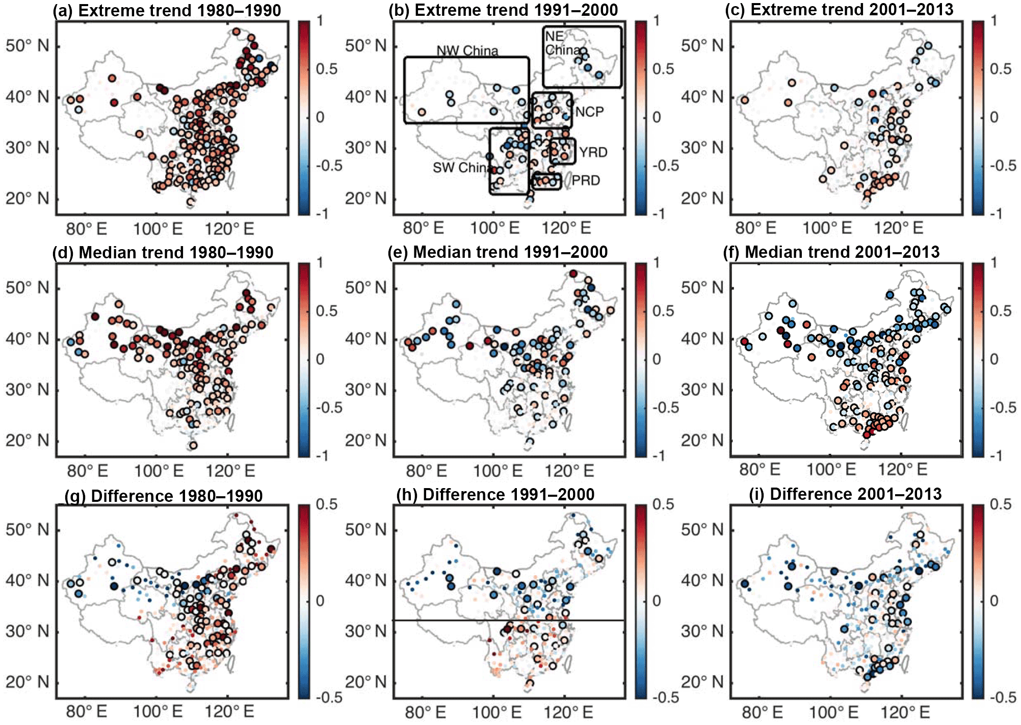
Figure 1 The first row: extreme trends estimated using quantile regression for the 3 decades: 1980–1990 (a), 1991–2000 (b), 2001–2013 (c). Panels (d–f): median trends estimated using quantile regression for the 3 decades. Panels (g–i): the difference between the values of the extreme trends and median trends, calculated as the extreme minus the median. All trends are unitless and expressed as relative changes.

The second approach is quantile regression, which is a well-established method used in many previous studies (Koenker and Hallock, 2001; Hannachi, 2006; Barbosa et al., 2011; Donner et al., 2012; Franzke, 2013) to estimate extreme trends in climate data.

For regular linear least square regression, the model can be expressed as

$$\begin{array}{}\text{(6)}& E\left[y\mathrm{|}\mathit{X}\right]=\mathit{\beta }\mathit{X}+\mathit{\epsilon },\end{array}$$

where y is the response variable conditioned on X, and β satisfies the minimization of the summed error function

$$\begin{array}{}\text{(7)}& \mathrm{err}=min\sum _i\mathit{\xi }(y_i-\mathit{\beta }{X}_i),\end{array}$$

where

$$\begin{array}{}\text{(8)}& \mathit{\xi }\left(u\right)=u^{\mathrm{2}}.\end{array}$$

For linear quantile regression, the response variable becomes the τth ($\mathit{\tau }\in [\mathrm{0},\mathrm{1}])$ quantile of y conditioned on X,

$$\begin{array}{}\text{(9)}& Q_{\mathit{\tau }}\left[y\mathrm{|}\mathit{X}\right]=\mathit{\beta }\mathit{X}+\mathit{\epsilon },\end{array}$$

where β still satisfies Eq. (2), but Eq. (3) now becomes

$$\begin{array}{}\text{(10)}& {\mathit{\xi }}_{\mathit{\tau }}\left(u\right)=\left\{\begin{array}{ll}u\mathit{\tau }& u\ge \mathrm{0}\\ u(\mathit{\tau }-\mathrm{1})& u<\mathrm{0}\end{array}.\right.\end{array}$$

Note that ξ_τ is symmetric when τ=0.5, rotated to the right when τ<0.5 and rotated to the left when τ>0.5. The quantile regression problem can be numerically solved by linear programming (Koenker and Hallock, 2001). Here, we use the R package “quantreg” to solve for the regression coefficients of daily mean AEC. Trends for both the 95th and 50th (median) percentiles are estimated, and the trends are compared. To test for significance of the quantile regression trends, we adopt the bootstrap approach proposed by Franzke (2013), who used surrogate data generated with the same autocorrelation function and the same probability density function as the original dataset. The detailed generation procedure can be found in Schreiber and Schmitz (1996) and Franzke (2013). Here, we generate 1000 surrogate time series to represent the intrinsic variability in the AEC time series.

In addition, we also calculate the trends for the median AEC (50th percentile) using the above two methods and compare them with the extreme trends. All trends are normalized and expressed as relative changes per decade, calculated as trend slope times the length of the time series divided by the corresponding AEC percentiles of the initial year. Therefore, the trends reported are unitless.

Figure S1 in the Supplement shows an example of the trend analysis using these two methods. In the following text, to save space, we only present trends using quantile regression, whereas the Sen's slope results, which agree well with the former, are presented in the Supplement.

3 Results

3.1 Trend maps

We first examine the distribution and temporal changes in trends for all sites in China. As indicated by Li et al. (2016), there are significant temporal shifts in the magnitude and sign of monthly mean AEC trends for different decades. We thus also examine the extreme and median trends for 3 consecutive decades: 1980–1990, 1991–2000 and 2000–2013. The overall trends for the 1980 to 2013 period are weakly positive for the majority of the sites (see Fig. S2).

The three columns in Fig. 1 show the distribution of extreme trend (panels a–c), median trend (panels d–f) and their differences (extreme minus median; panels g–i) for the 272 sites for the three periods. To avoid the confusion caused by positive and negative signs of the trend, the differences here are calculated using the absolute value of the extreme and median trends. Larger dots in black circles mean that the trends are statistically significant at the 95 % level. Figure 1 is the result from quantile regression, whereas the trends using Sen's slope are presented in Fig. S3, which shows a largely consistent pattern. It is seen from Fig. 1 that the sign of median and extreme trends mostly agrees throughout China. An extensive positive trend is observed all over China in the 1980s. During the 1990s, many sites, especially those in north China, began to experience a decreased AEC. After the year 2000, the north China sites continue to show decreasing trends, whereas AEC over many south China sites started to rise again.

However, a detailed comparison between median and extreme trends reveals distinct spatial and temporal differences. Focusing on the bottom three panels of Fig. 1g–i, it is clear that in the 1980s, the extreme trends exceed the median trend throughout China, with some differences as large as 50 % (northwestern sites). The number of sites showing a significant extreme trend (178) is also greater than those with a significant median trend (91). Note that the number of significant sites can be different between quantile regression and Sen's slope results because (1) quantile regression is applied to daily data, while Sen's slope uses annual or seasonal percentiles, and (2) quantile regression uses a bootstrap method to test for significance, while Sen's slope uses an MK test. Nonetheless, the spatial patterns of the two methods are consistent. In the 1990s, the distribution of the trend differences switched to a north–south “dipole” pattern, with negative values in the north and positive ones in the south in general; i.e., extreme trends are weaker than the median trend in the north but stronger in the south, with a rough separation at 33 ^∘N marked by the horizontal black line in Fig. 1h. In the north, the sites showing significant extreme trends also become fewer than those with significant median trends in the north. Even in the south, the difference between the extreme and median trends is much smaller compared to the 1980s, indicating a slowdown of the increase in the extreme values. After the year 2000, almost all of China exhibits a “blue” pattern as opposed to the “red” pattern in the 1980s. Except for a few sites in central south China, the majority exhibits a weaker extreme trend than the mean trend. There are also fewer sites showing significant trends in the extreme (52) than in the median (119). This feature is particularly strong for northeast, northwest and south China. Although east and south China still show positive AEC trends, this result suggests that in this decade, the extreme pollution conditions have not increased as much as the mean or background pollution.

In short, the positive trends in the 1980s over China can be primarily attributed to an increase in the extremes. The 1990s experienced a transition, with the extreme trends becoming weaker than the median trend in the north and only slightly stronger in the south. Finally in the 2000s, the extreme trends largely yield to the median trends.

Figure 2 Probability distribution function (pdf) of AEC (Mm⁻¹) for the 3 decades over the six representative regions marked in Fig. 1b. The AEC has been converted to logarithmic scale.

3.2 Regional trends

To examine the spatial and temporal changes in more detail, we further divide the country into six representative regions, marked by black rectangles in Fig. 1b. Three of these regions – the North China Plain (NCP), the Yangtze River Delta (YRD) and the Pearl River Delta (PRD) – are the major urban conglomerates in China. Since the change in the extreme and median is essentially related to the shift in the distribution, we first evaluate the regional AEC (/Mm⁻¹) distributions for the 3 decades. Figure 2 plots these distributions by region on logarithmic scale, as AEC is usually considered to follow a lognormal distribution (Collaud Coen et al., 2013). The dashed lines in Fig. 2 indicate the location of the 95th percentile. For all regions, there is a rightward extension of the tail of the distribution from the 1990s to the 1980s, implying an increase in the extremes, which is also characterized by the rightward shift in the 95th percentile line. NCP, YRD and NW China also show a rightward shift in the distribution peak. From 1990s to 2000s, although the distribution peak shifts to the right for PRD, YRD, SW China and NE China, there is no obvious shift in the tail for these four regions. For the other two regions – NCP and NW China – there is a leftward shift in both the peak and the tail, but the shift in the peak is stronger. Overall, we can roughly conclude that the 1980s AEC trend is characterized by a change in the extremes, while in the 2000s the median dominates the trend.

Consistent with Li et al. (2016), we also calculate trends successively for all periods starting each year from 1980 to 2004 and ending in 2013 with 10-year increments. Figure 3 shows the temporal evolution of the quantile regression trend differences with the x axis indicating the trend calculation start year and the y axis indicating the length of the time series, with its counterpart using Sen's slope shown by Fig. S4. To save space, only the absolute differences between the extreme and median trends are presented in Fig. 3, while their respective values are shown in Figs. S5 and S6 for quantile regression and Figs. S7 and S8 for Sen's slope. Table 1 displays the regional extreme and median trends using the two methods and their differences for the three periods: 1980–1990, 1991–2000 and 2001–2013. Note although the absolute values of Sen's slope and quantile regression trends can be different, their signs are consistent. The time series and linear trends for each region are presented in Fig. S9. Because in Fig. 3 the trends are calculated successively for each period, it helps to examine the time node of the changes more precisely. For example, although Figs. 1 and 2 both indicate that the extremes increase more rapidly in the 1980s, for YRD and PRD, the duration is short with the extreme trend exceeding the median trend since around 1982, while for the other four regions the change happened around 1986 or later. YRD, PRD and NE China experienced a short period of a stronger extreme trend from ∼ 1994 to 1996, whereas the other three regions show weaker extreme trends. After 2002, SW and NW China display a slightly higher extreme trend, which is different from the other four regions. These features suggest that there can be minor differences when the trends are examined for different time periods.

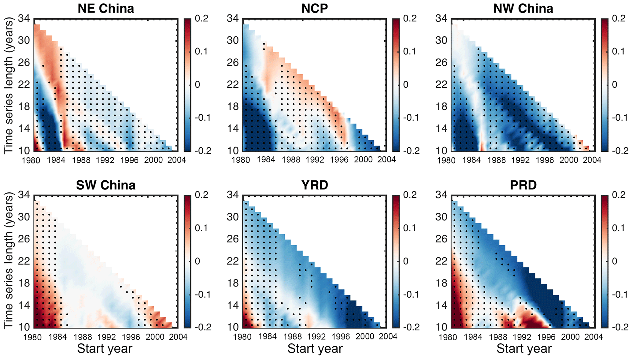
Figure 3 Difference between extreme and median trends calculated using quantile regression for the six representative regions marked in Fig. 1b. Trends are between each year from 1980 to 2004 and the end of the record, with a 10-year minimum required to calculate the trend. The x axis indicates the starting year, and the y axis indicates the length of the time series to calculate the trend.

The seasonal time series of the difference between extreme and median quantile regression trends are plotted in Fig. 4, with a 4-year moving average to smooth out small wrinkles (its counterpart using Sen's slope is shown in Fig. S10). Note that Fig. 4 shows the evolution of the trend difference for every 10-year period from 1980 to 2004 (i.e, 1980–1989, 1981–1990, ..., 2004–2013). An outstanding feature in Fig. 4 is that for all regions, the summer (JJA) trend difference (indicated by red curves) exhibits quite different, or even reversed, variability from the other three seasons and the annual result. For NE, NW China and the PRD, spring (MAM) trends also have relatively larger departure. In general, winter (DJF) and fall (SON) trends agree better with the annual trend. Since these two seasons are dominated by anthropogenic aerosols such as sulfate, nitrate, and black and organic carbon throughout China (Cao et al., 2007; Wang et al., 2007, 2015), the results indicate that changes in anthropogenic aerosol loading are primarily responsible for the observed extreme and median trends. In the spring many regions are influenced by dust, and in the summer, the relative humidity effect may significantly enhance aerosol extinction. Both are natural factors and should have a minor contribution to the annual trend according to Fig. 4.

4 Conclusions and discussion

While the trends in aerosol pollution in China have been studied extensively, it remains to be understood whether the extreme conditions have changed and whether their changes are faster or slower than the mean. In this study, we use a quality-controlled visibility dataset to examine decadal trends in extreme values of surface aerosol extinction coefficients. Quantile regression and Sen's slope estimates are jointly used to estimate the trends to improve its robustness. Our analysis reveals that, in general, the extreme and median trends agree in terms of the sign but they can differ significantly in terms of the amplitude. During the 1980s, the extremes increased faster than the median for most of China except for a few north and northwest sites. The 1990s experienced a transition with the extreme trend becoming weaker than the median trend in the north but still remaining slightly stronger in the south. Then in the 2000s, the majority of the country exhibited a weaker extreme trend than the median trend. Seasonally, winter and fall trends are the most consistent with annual trends, while the summer trend shows the largest departure from the annual trend.

Table 1 Regional extreme and median trends.

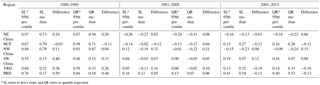
* SL refers to Sen's slope, and QR refers to quantile regression

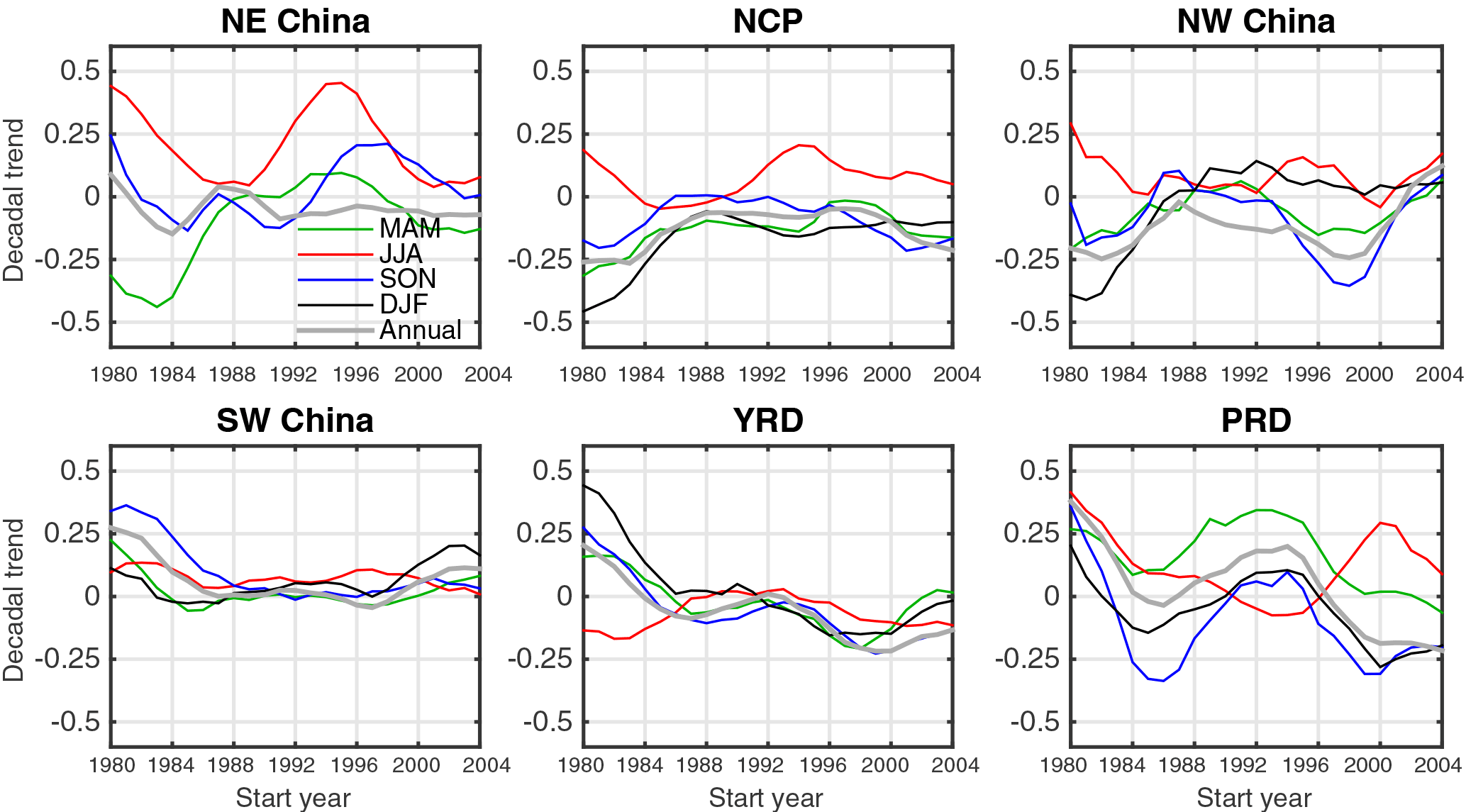
Figure 4 Seasonal time series of the difference between the extreme and median trends. The trends are calculated for each 10-year period starting from 1980 to 2004 (x axis), i.e., the first point is the trend difference for the 1980 to 1989 period, the second from 1982 to 1990, etc.

This study uses daily mean daytime AEC without accounting for its diurnal variability. Nonetheless, visibility can still change considerably in the course of a day (Deng et al., 2011). To examine this effect we repeat the analysis using daily minimum and daily maximum AEC. The counterparts of Fig. 1 are shown in Figs. S11 and S12. A brief comparison indicates a high resemblance of these two figures to Fig. 1, which uses daily mean data, albeit with some reasonable differences in the amplitude.

The reason for the different behaviors in the extreme and median trends still needs further investigation and will be the topic of our future study. One implication is that in the 1980s and part of the 1990s, synoptic conditions might have been playing a major role in modulating aerosol variability. For example, several extremely heavy pollution events are believed to be linked to stagnant weather (Tao et al., 2014; Zheng et al., 2015). After the mid-1990s, emission might have become more dominate, which tends to increase both the extreme and the mean. But since it is a relatively uniform background change, the signal might be more prominent in the mean condition. On the other hand, aerosol properties can also be potentially influenced by decadal or interannual climate variability (Chen and Wang, 2015; Wang and Chen, 2016), whose footprint may be embedded in these extreme and mean trends. However, the mechanism by which they have an impact on the extremes and the mean still needs to be understood and likely requires a comprehensive study using both observations and model simulations. This also requires the models to accurately simulate the extreme events, which is a challenging task.

Admittedly, the visibility data are not ideal for aerosol-related studies, given their various sources of uncertainties as discussed in Li et al. (2016). However, it is currently best compromise since there is lack of reliable long-term aerosol observation datasets. Moreover, remote-sensing products are vulnerable to extreme pollution, making them unsuitable for extreme trend studies. For example, as discussed in Lin and Li (2013), MODIS frequently misses the heavy haze over north China, likely due to the cloud screening algorithm. Sun photometers will also stop working when the sun is blocked by the heavy pollution. This also suggests that current remote-sensing instruments and retrieval algorithms need to be improved to observe these extreme events.