Model simulations of the chemical and aerosol microphysical evolution of the Sarychev Peak 2009 eruption cloud compared to in situ and satellite observations

Volcanic eruptions impact climate through the injection of sulfur dioxide (SO₂), which is oxidized to form sulfuric acid aerosol particles that can enhance the stratospheric aerosol optical depth (SAOD). Besides large-magnitude eruptions, moderate-magnitude eruptions such as Kasatochi in 2008 and Sarychev Peak in 2009 can have a significant impact on stratospheric aerosol and hence climate. However, uncertainties remain in quantifying the atmospheric and climatic impacts of the 2009 Sarychev Peak eruption due to limitations in previous model representations of volcanic aerosol microphysics and particle size, whilst biases have been identified in satellite estimates of post-eruption SAOD. In addition, the 2009 Sarychev Peak eruption co-injected hydrogen chloride (HCl) alongside SO₂, whose potential stratospheric chemistry impacts have not been investigated to date. We present a study of the stratospheric SO₂–particle–HCl processing and impacts following Sarychev Peak eruption, using the Community Earth System Model version 1.0 (CESM1) Whole Atmosphere Community Climate Model (WACCM) – Community Aerosol and Radiation Model for Atmospheres (CARMA) sectional aerosol microphysics model (with no a priori assumption on particle size). The Sarychev Peak 2009 eruption injected 0.9 Tg of SO₂ into the upper troposphere and lower stratosphere (UTLS), enhancing the aerosol load in the Northern Hemisphere. The post-eruption evolution of the volcanic SO₂ in space and time are well reproduced by the model when compared to Infrared Atmospheric Sounding Interferometer (IASI) satellite data. Co-injection of 27 Gg HCl causes a lengthening of the SO₂ lifetime and a slight delay in the formation of aerosols, and acts to enhance the destruction of stratospheric ozone and mono-nitrogen oxides (NO_x) compared to the simulation with volcanic SO₂ only. We therefore highlight the need to account for volcanic halogen chemistry when simulating the impact of eruptions such as Sarychev on stratospheric chemistry. The model-simulated evolution of effective radius (r_eff) reflects new particle formation followed by particle growth that enhances r_eff to reach up to 0.2 µm on zonal average. Comparisons of the model-simulated particle number and size distributions to balloon-borne in situ stratospheric observations over Kiruna, Sweden, in August and September 2009, and over Laramie, USA, in June and November 2009 show good agreement and quantitatively confirm the post-eruption particle enhancement. We show that the model-simulated SAOD is consistent with that derived from the Optical Spectrograph and InfraRed Imager System (OSIRIS) when both the saturation bias of OSIRIS and the fact that extinction profiles may terminate well above the tropopause are taken into account. Previous modelling studies (involving assumptions on particle size) that reported agreement with (biased) post-eruption estimates of SAOD derived from OSIRIS likely underestimated the climate impact of the 2009 Sarychev Peak eruption.

1 Introduction

Explosive volcanic eruptions inject large quantities of sulfur dioxide (SO₂) into the atmosphere and have the potential to affect global climate (McCormick et al., 1995; Robock, 2000). Volcanic eruptions impact the global radiative budget via the formation of sulfuric acid aerosol particles from the volcanic SO₂ emitted. The presence of this particle load at stratospheric altitudes enhances the stratospheric aerosol optical depth (SAOD) and increases the solar backscatter, thereby inducing a cooling at the Earth's surface. The lifetime of sulfuric acid aerosol particles in the stratosphere can reach several years, significantly longer than in the troposphere (days to weeks). Large-magnitude eruptions that inject SO₂ directly into the stratosphere therefore typically have more prolonged and widespread (global or hemispheric) impacts than small-magnitude eruptions that typically inject SO₂ into the troposphere only. The June 1991 eruption of Mount Pinatubo was a large-magnitude eruption, with a volcanic explosivity index (VEI, as defined in Newhall and Self, 1982) of 6, that had a significant impact on the stratospheric aerosol layer and hence climate (Ammann et al., 2003; Bluth et al., 1992; Sato et al., 1993): global aerosol optical depth (AOD) (in the visible) was enhanced, reaching up to 0.15, causing a surface cooling of up to 0.5 ^∘C (Douglass and Knox, 2005; Wunderlich and Mitchell, 2017). In addition, stratospheric halogens (bromine and chlorine, which are present at elevated post-industrial concentrations in the stratosphere as a consequence of past anthropogenic chlorofluorocarbon (CFC) emissions) became activated through reactions on the volcanic aerosol, causing substantial depletion of stratospheric ozone and larger polar ozone holes (Portmann et al., 1996; Solomon et al., 1996; Tilmes et al., 2008).

Moderate-magnitude explosive volcanic eruptions may also reach the stratosphere. However, they typically have a much reduced effect on climate and atmospheric chemistry compared to large-magnitude eruptions (Kravitz et al., 2010; Oman et al., 2005). In general, a smaller mass of SO₂ is injected and oxidized to sulfate aerosol. Also, by injecting to lower altitudes, the emissions from moderate-magnitude eruptions are more susceptible to removal by stratospheric–tropospheric exchange processes (Haywood et al., 2010). Nevertheless, as volcanic eruption frequency follows an inverse power law with magnitude (Sparks, 2003), the cumulative impacts of frequent moderate-magnitude eruptions on stratospheric aerosol can be significant (Vernier et al., 2011) and, for example, were identified as a factor in recent decadal climate trends (Ridley et al., 2014; Solomon et al., 2011).

Here, we study the moderate-magnitude eruption of Sarychev Peak volcano, which erupted in mid-June 2009 in the Kuril Islands, Russia (48^∘ N, 153^∘ E, 1512 $\mathrm{m}\mathrm{a}.\mathrm{s}.\mathrm{l}.$), injecting SO₂, ash, and also HCl to the stratosphere. The eruption was classified with a VEI of 4 (the volcanic eruptive index as defined in Newhall and Self (1982) is a logarithmic scale based on the volume of tephra ejected), and the main volcanic emission was injected into heights around 9–14 km as estimated from Infrared Atmospheric Sounding Interferometer (IASI) retrievals (Carn et al., 2016; Carboni et al., 2016). Remote sensing observations over Eureka, Canadian Arctic, showed volcanic aerosol layers from the tropopause up to 16–17 km 1 month after the eruption, that subsequently settled into a more homogeneous layer in the lower stratosphere (O'Neill et al., 2012).

Previous modelling studies of the Sarychev 2009 eruption focused on the injection of SO₂, formation of volcanic aerosol, and its radiative and atmospheric chemistry impacts (Berthet et al., 2017; Haywood et al., 2010; Kravitz et al., 2011). However, the models did not explicitly simulate the aerosol microphysical evolution of the volcanic cloud; rather, they used bulk aerosol schemes and/or assumed size distributions. Model-simulated atmospheric impacts of the eruption on, for instance, aerosol optical depth, are highly dependent on the prescribed aerosol size (or effective radius, r_eff). An r_eff of 0.13 µm was assumed in the HadGEM2 model study by Haywood et al. (2010), whilst Kravitz et al. (2011) used scaling to adjust their ModelE (Schmidt et al., 2006) simulations to represent a similar r_eff. Measurements that locally quantified the post-eruption volcanic aerosol include ground-based remote sensing (Haywood et al., 2010; Kravitz et al., 2011; Mattis et al., 2010; O'Neill et al., 2012) and balloon-borne observations. For example, Kravitz et al. (2010) and Jégou et al. (2013) present in situ balloon-borne observations of size-resolved stratospheric aerosol over Laramie, Wyoming, USA (June and November 2009), and Kiruna, Sweden (August–September 2009), respectively. The estimates of r_eff from all these measurements range from 0.1 to 0.3 µm, i.e. larger than assumed in the models. Further evidence for a larger particle size comes from an effective radius estimate of 0.1–0.3 µm derived from satellite-based observations 1 month after the eruption (Doeringer et al., 2012) and a particle “sedimentation radius” of 0.5–1 µm from a model sensitivity study (Günther et al., 2017).

O'Neill et al. (2012) highlight that this discrepancy can translate into large uncertainties in the modelled impacts; e.g. doubling of particle size from that assumed by Haywood et al. (2010) would lead to a 5-fold increase in the hemispherical (per particle) backscattering cross section of sulfate particles.

Volcanic aerosol from the Sarychev eruption also affected stratospheric halogen chemistry via heterogeneous reactions on the aerosol surface area. The impacts were more modest than found for large-magnitude eruptions such as the 1991 Mt. Pinatubo eruption, but simulations suggest ozone depletion up to 4 % in the lower stratosphere at high latitudes, with local NO₂ depletion up to 40 % (Berthet et al., 2017), consistent with balloon-based and satellite observations (Adams et al., 2017).

To evaluate and tune the models, studies to date have relied upon satellite data from the Optical Spectrograph and Infrared Imaging System (OSIRIS) instrument to provide a global estimation of aerosol optical depth. However, comparison between OSIRIS and the models found a ≈1-month discrepancy in the timing of the SAOD maximum following the eruption. This was attributed to be likely due to deficiencies in the model aerosol microphysics, specifically the absence of nucleation processes (Haywood et al., 2010; Jégou et al., 2013). In subsequent work, Fromm et al. (2014) identified that stratospheric AOD derived from OSIRIS under high aerosol loadings was likely underestimated following volcanic eruptions, due to a saturation effect and because the extinction profiles may terminate well above the tropopause (and therefore miss volcanic aerosol in the lowermost stratosphere). More generally, underestimation of SAOD due to neglect of lower stratospheric volcanic aerosols has also been highlighted by Andersson et al. (2015); Kravitz et al. (2011); Mills et al. (2016); Ridley et al. (2014). As model studies to date have used OSIRIS-derived AODs to evaluate and justify choice of model aerosol parameters such as r_eff (Haywood et al., 2010; Kravitz et al., 2011), this finding invokes the need to reexamine the assumed volcanic aerosol properties in the models. Finally, there have also been recent advances in satellite observations of volcanic gases in the stratosphere. First, new retrievals now enable an improved estimation of SO₂ mass injected combined with estimates of plume height from IASI on the MetOp-A satellite (Carboni et al., 2016; Clarisse et al., 2012). Second, recent analysis of satellite data from the Microwave Limb Sounder (MLS) aboard the Aura satellite identifies that the Sarychev volcano co-injected HCl alongside SO₂ into the stratosphere (Carn et al., 2016). The co-injection of volcanic halogens alongside SO₂ could modify the resulting atmospheric chemistry/aerosol processing and impacts. In light of these advances, it is instructive to perform a new model–observation study of the Sarychev 2009 eruption and its stratospheric impacts that furthermore benefits from recently developed model capabilities to simulate aerosol microphysics and size evolution.

Here, we present model simulations of stratospheric aerosol evolution and chemistry following the moderate-magnitude 2009 Sarychev eruption using the global Community Earth System Model version 1.0 (CESM1) (Marsh et al., 2013), with its Whole Atmosphere Community Climate Model (WACCM) module for the simulation of the atmosphere, along with the sectional Community Aerosol and Radiation Model for Atmospheres module (CARMA; Toon et al., 1988) to simulate aerosol microphysics. The sectional scheme distributes particles according to their size over 30 size bins, enabling the evolution of the particle size distribution to be traced in detail with no a priori assumptions on particle size. This model with sectional aerosol was previously used by English et al. (2013) to evaluate aerosol evolution and multi-year impacts from the large-magnitude eruptions of the 1991 Pinatubo eruption and the 100 times stronger Toba eruption (74 000 years before present). Aerosol impacts from large-magnitude eruptions are substantial but limited by particle growth and sedimentation (with a 20-fold increase in AOD following Toba compared to Pinatubo despite its 100-fold increase in SO₂ injection). The globally averaged effective radius reached 0.45 and 1.9 µm after the Pinatubo and Toba eruptions, respectively. English et al. (2013) highlight the need to simulate microphysical processes and advantages of a sectional aerosol representation for a more comprehensive understanding of aerosol evolution following volcanic eruptions. This motivates our study, which applies a sectional aerosol microphysics modelling approach to simulate aerosol evolution following a moderate-magnitude eruption.

The aims of our study are (i) to simulate the stratospheric aerosol evolution following the 2009 Sarychev eruption using a model that explicitly accounts for aerosol microphysical processes using a sectional aerosol scheme, in order to deliver the first model simulations of the size-resolved stratospheric aerosol evolution to assess impacts following the Sarychev eruption; (ii) compare the model output to balloon-based in situ measurements of size-resolved aerosol and to satellite observations of aerosol optical depth, accounting for reported measurement limitations, in order to deliver an improved model assessment of the aerosol impact in the 12 months following the Sarychev eruption; and (iii) to investigate to what extent co-injection of HCl alongside SO₂ may have influenced the subsequent stratospheric aerosol processing and atmospheric chemistry impacts.

2 Methods

2.1 The CESM1(WACCM)-CARMA model: initialization, set-up, and data post-processing

Model simulations were performed using the global CESM1 using its WACCM module linked to the CARMA module, involving the sulfur cycle with a sectional aerosol scheme (English et al., 2011). Land, sea ice, and rivers were active modules, whereas oceans were data prescribed. The spatial resolution was a longitude/latitude grid of 144 points by 96, respectively (i.e. approximately 2^∘ resolution), and over 88 levels of altitude ranging from the ground to approximately 150 km altitude with approximately 20 levels in the troposphere. Specified dynamics were used, with a nudging towards the Modern-Era Retrospective analysis for Research and Applications (MERRA) meteorological data (Rienecker et al., 2011) at every time step (30 min) with a weight factor of 0.1 towards the analysis, for temperature and wind fields. The following surface emissions were prescribed in the model. For SO₂, NH₃, black carbon, organic carbon, NO_x, CH₄, and CO emissions, the MACCity data set was used (van der Werf et al., 2006; Lamarque et al., 2010; Granier et al. 2011; Diehl et al., 2012). Anthropogenic CH₄ emissions were added from the EDGAR v4.2 database (available at http://edgar.jrc.ec.europa.eu); biogenic CO emissions were added from the Model of Emissions of Gases and Aerosols from Nature – Monitoring Atmospheric Composition and Climate (MEGAN-MACC) database (Sindelarova et al., 2014). Carbonyl sulfide (OCS) was prescribed using data from Kettle et al. (2002). CH₂O was prescribed according to the IPCC RCP8.5 scenario (Riahi et al., 2011), and for H₂ the ECCAD-GFED3 database was used (van der Werf et al., 2010). For CO₂, N₂O, CCl₄, CF₂ClBr, CF₃Br, CH₃Br, CH₃CCl₃, CH₃Cl, CFC11, CFC113, CFC12, and HCFC22 emissions, lower boundary conditions were prescribed following CCMI/RCP8.5 data.

Simulations were started on 1 January 2009, using the CESM1(WACCM) initial atmosphere state file at that date. This enabled a 6-month model spin-up period before the eruption injection on 15 June 2009, after which the simulations were continued for 1 year, ending on 31 May 2010. The Sarychev Peak eruption was simulated by injecting volcanic SO₂ (and HCl) gases into model grid boxes corresponding to the location of the volcano (48^∘ N, 153^∘ E), over the duration of 15 June 2009, spread evenly between 11 and 15 km altitude a.s.l.. The model's 2.5^∘ longitude $\times \mathrm{1.875}{}^{\circ }$ latitude grid resolution means that the volcanic plume is initially too dilute in the model compared to reality. This is nevertheless a common methodology; see, e.g. Haywood et al. (2010). The vertical distribution of our SO₂ injection follows previous model studies. It is a somewhat coarse approximation given that O'Neill et al. (2012) report lidar observations of fine-scale aerosol layers shortly after the eruption. Nevertheless, these were subsequently observed to collapse into a single layer in the lower stratosphere. For the magnitude of the SO₂ injection, we use a revised estimate in contrast to previous studies, as discussed below.

A detailed chronology of the Sarychev Peak 2009 eruption can be found in Levin et al. (2010), which identified three explosive periods: on 12–13 June, repeated explosions occurred, reaching heights ranging from 5 to 10 km; an isolated, high-altitude explosion occurred on 14 June, reaching 21 km altitude; finally, on 15 June, a series of consecutive explosions reached altitudes ranging between 10 and 15 km (all times are in UTC). The first eruptive clouds on the 11–14 June period were mainly ash (Rybin et al., 2011). We neglected the minor, low-altitude (inferior to 5 km) explosions reported on 11 and 16 June, and injected SO₂ continuously for a 24 h period on 15 June spread evenly between 11 and 15 km altitude a.s.l.. The timing of the SO₂ emissions is based on SO₂ satellite retrievals from IASI (Carboni et al., 2016; Carn et al., 2016; Clarisse et al., 2012), MODIS (MODerate-resolution Imaging Spectroradiometer; Realmuto and Berk, 2016; Rybin et al., 2011), and OMI (Ozone Monitoring Instrument; Theys et al., 2015), which all show that the majority of high altitude SO₂ was released on 15 June (and possibly in the early morning of 16 June). Haywood et al. (2010) used a total injection mass of 1.2 Tg SO₂, which was the SO₂ total mass value retrieved on 16 June with IASI. An update of the SO₂ algorithm (Clarisse et al., 2012) found a maximum SO₂ mass value of around 0.9 Tg, a value which was confirmed with subsequent updates of that algorithm (Carn et al., 2016). It is also consistent with retrievals from OMI (Theys et al., 2015) and MODIS (Realmuto and Berk, 2016). In contrast, the IASI retrievals reported in Carboni et al. (2016) found that the transient SO₂ burden reached only up to 0.6 Tg SO₂. We consider though that 0.9 Tg of SO₂ is the best estimate for the mass of SO₂ injected by the Sarychev eruption into the UTLS. We did not consider any ash emissions.

In a second simulation, 27 Gg HCl was co-injected alongside the 0.9 Tg of SO₂. This initialization follows the recent identification of a localized stratospheric HCl enhancement following the Sarychev eruption (Carn et al., 2016), based on analysis of Microwave Limb Sounder (MLS) satellite observations, reporting a HCl∕SO₂ mass ratio of around 3 %. Since the low vertical resolution of MLS in the lower stratosphere makes it difficult to infer the precise injection altitude of HCl, we assumed an HCl injection altitude identical to that of SO₂. A control run without the volcanic gas injection was also performed, enabling anomalies to be calculated. In the present paper, we will refer to control runs as “volcano-off” simulations and to runs including the eruption as “volcano-on” simulations.

The CESM1(WACCM) atmospheric chemistry scheme includes a detailed sulfur cycle and key stratospheric nitrogen (NO_y), and halogenated (i.e. chlorine and bromine) and hydrogenated (in particular HO_x radicals) compounds. The formation and microphysics of sulfuric acid aerosol particles simulated by the CARMA module are described in detail in English et al. (2011).

The CARMA module in sectional configuration yields particle concentration across 30 size bins ranging from approximately 0.68 nm to 3.25 µm in dry diameter. Effective radius is also provided as a direct model output. Post-processing of the model output was used to determine wet particle size distributions, extinctions, and optical depth. In each model grid cell, the wet diameter of each size bin was calculated using a (hygroscopic growth) parameterization of H₂SO_4(aq) particle volume as a function of acid weight percentage (wt %H₂SO₄), ambient humidity, and temperature following Tabazadeh et al. (1997). Extinctions at 750 and 550 nm were calculated by combining the particle concentrations across the sectional size bins with the corresponding wet radii and particle refractive indices following Beyer et al. (1996), using a Mie scattering code at the desired wavelength (van de Hulst and Twersky, 1957). The aerosol extinctions were integrated with altitude over the stratosphere to yield SAOD.

2.2 Balloon-borne in situ and satellite-based remote sensing observations of aerosol and SO₂

The model SO₂ output (from simulations with and without HCl co-injection) is compared to vertical columns of SO₂ and total (northern hemispheric) SO₂ burden derived from IASI. The Infrared Atmospheric Sounding Interferometer is an instrument that has been present aboard the MetOp-A satellite since the end of 2006. It is a spectrometer measuring infrared light spectra at nadir. Its primary goal is to assess temperature and water vapour content of the atmosphere, but it can also be used to retrieve the atmospheric concentrations of various gases, including SO₂ (Carboni et al., 2016; Clarisse et al., 2008). IASI provides global coverage twice a day, and its footprint ranges from circular (12 km diameter at nadir) to elliptical (up to 20 km by 39 km at the end of the swath). For this comparison, we use the IASI retrieval of SO₂ by Clarisse et al. (2012). The IASI data set and retrieval algorithm used for this precise eruption can be considered as showing a lower threshold of around 0.3 DU, and SO₂ loads can be expected to have a 10–20 % uncertainty. IASI altitude retrievals have a typical sensitivity of 1–2 km. We also compare our results to HadGEM2 model simulations of SO₂ and earlier IASI SO₂ retrievals reported by Haywood et al. (2010).

Comparisons of the modelled aerosols with in situ measurements are two-fold. First, we compare the model's output with size-resolved aerosol measurements carried out with the balloon-borne Stratospheric and Tropospheric Aerosol Counter (STAC) optical particle counter (OPC) instrument over Kiruna, Sweden, on 2, 7, and 18 August 2009, and 18 May 2010. STAC can be borne under stratospheric balloon gondolas and can measure low concentrations in aerosols down to approximately 10⁻⁴ ${\mathrm{cm}}^{-\mathrm{3}}\mathrm{\mu }{\mathrm{m}}^{-\mathrm{1}}$ (Ovarlez and Ovarlez, 1995; Renard et al., 2005, 2010). Particles are classified by their diameters into tuneable size bins ranging from a few tenths of micrometre to a few micrometres. The counts in each size bin are normalized by the bin width to yield a size distribution. The uncertainty, defined as the relative standard deviation (SD), is 60 % for aerosol concentrations of 10⁻³ cm⁻³, 20 % for 10⁻² cm⁻³, and 6 % for concentrations higher than 10⁻¹ cm⁻³. STAC was operated successfully on eight different balloon flights throughout the August–September 2009 period over Kiruna, Sweden (68^∘ N, 20^∘ E), as part of the StraPolÉté campaign (French acronym for Stratosphère Polaire en Été), and also in May 2010, as part of the AEROWAVE project (acronym for AEROsols, WAter Vapour and Electricity). Measurements of the STAC instruments are available online at https://cds-espri.ipsl.upmc.fr. During these flights, it was demonstrated that STAC passed through the Sarychev plume (Jégou et al., 2013), as explored further in the present paper. Our comparison focuses on the submicron range between ≈0.3 and 1 µm diameters. We have performed an interpolation of the counts from the model's size bins to the STAC size bins (and from the model pressure levels to the observed pressure of the balloon payload) in order to enable a direct comparison.

Second, we also compare the model's aerosol output with in situ measurements carried out by the OPC of the University of Wyoming (Deshler et al., 2003), flown on stratospheric balloons launched from Laramie, USA (41^∘ N, 105^∘ W), on 22 June 2009 and 7 November 2009 (Kravitz et al., 2011). For comparison to the model, total particle number above two diameter threshold sizes is considered here: d> 20 nm (condensation nuclei, CN) and d>0.5 µm (nuclei, N). Uncertainties are 85, 25, and 8 % for concentrations of 10⁻³, 10⁻², and 10⁻¹ cm⁻³, respectively (Deshler et al., 2003). These data are available from ftp://cat.uwyo.edu/pub/permanent/balloon/Aerosol_InSitu_Meas/US_Laramie_41N_105W/. They have been derived by the University of Wyoming as follows: the measurement of N is calculated directly from the OPC instrument. The CN is derived from a condensation nuclei counter co-deployed on the balloon payload. Note that both STAC and University of Wyoming OPCs have been compared by Renard et al. (2002).

Model SAOD was compared to that derived from extinction measurements by the OSIRIS aerosol instrument (aboard the Odin satellite). OSIRIS is a limb sounder that is able to provide information on the vertical distribution of atmospheric aerosols (Bourassa et al., 2007, 2008) from the upper troposphere up to the lower mesosphere through the analysis of scattered sunlight. This Canadian instrument has been active since November 2001 aboard the Swedish satellite Odin (Llewellyn et al., 2004). Its global coverage reaches up to 82^∘ in latitude. Odin evolves on a Sun-synchronous orbit, and therefore the availability of OSIRIS's measurements is latitude and time dependent. Our analysis focuses on extinction measurements from OSIRIS version 5.07, available from http://odin-osiris.usask.ca/. Importantly, a novel aspect of our study is that our analysis specifically accounts for instrument errors or limitations as reported by Fromm et al. (2014). Model output data have been degraded accordingly. First, the modelled extinctions have been made to saturate at an upper threshold of $\mathrm{2.5}\times {\mathrm{10}}^{-\mathrm{3}}$ km⁻¹; then, extinctions have been only integrated above a certain altitude, dependent on the latitude: a linear variation of this lower limit was assumed from 0.5 km above the tropopause at the Equator up to 5.5 km above the tropopause at the poles. Further details are given in Sect. 3.4.

3 Results

3.1 Spatial and temporal evolution of volcanic SO₂ vertical column densities

Figure 1 shows vertical column densities of SO₂ from the CESM1(WACCM) simulation in which both volcanic SO₂ and HCl were injected (Fig. 1b) and a comparison with IASI retrievals (Fig. 1a). Both sets of maps are shown with the same lower threshold in terms of Dobson units, corresponding to an estimated lower threshold of 0.3 DU in IASI's retrievals for this precise eruption and for the IASI retrieval algorithm used (Clarisse et al., 2012). The spatial and temporal evolution of the Sarychev SO₂ plume is reasonably well simulated by the CESM1(WACCM) runs throughout the first fortnight following the eruption. There are some notable discrepancies, for instance, on 16 June 2009 south-west of Alaska: this is likely due to our simulation not accounting for the small amount of SO₂ that was emitted before the main eruption on 15 June 2009. Also, Asian pollution (close to 0.3 DU) is evident in the simulations shown in Fig. 1 but not observed by IASI, likely due to the reduced sensitivity of the IASI retrievals to SO₂ below 5 km altitude. To quantify the spatial-amplitude match between the two sets of data, we chose a colocation index calculated as

$$\begin{array}{}\text{(1)}& \mathit{\rho }={\displaystyle \frac{\mathbb{E}\left[\right(P_{\mathrm{1}}-{\mathit{\mu }}_{\mathrm{1}}\left)\right(P_{\mathrm{2}}-{\mathit{\mu }}_{\mathrm{2}}\left)\right]}{{\mathit{\sigma }}_{\mathrm{1}}{\mathit{\sigma }}_{\mathrm{2}}}},\end{array}$$

where P₁ and P₂ are the two-dimensional matrices representing the spatial SO₂ loads (for model and satellite retrievals), sampled over the same spatial grid, and stacked into one-dimensional vectors; μ_{1;2} and σ_{1;2} are their respective means and SDs. It is expected that the index drops quite quickly after the eruption due to greater dispersion in the model on the 2×2 degree grids than in the finer-scale (tens of kilometres) IASI observations. Colocation indices were calculated over the first fortnight following the eruption (Table 1) for the simulation with SO₂ injection only and with HCl co-injection alongside SO₂. As can be noted from Table 1, colocation indices show comparable values for both model runs. This indicates broadly similar SO₂ dispersion in the model runs.

The spatial and temporal evolution of the plume in our study is consistent with the results of Wu et al. (2017), where AIRS data are presented along with results of simulations by a particle dispersion model.

Table 1 Colocation indices quantifying the spatial-amplitude agreement in the volcanic SO₂ vertical column densities simulated by CESM1(WACCM) compared to IASI observations over the Northern Hemisphere for 1–2 weeks after the eruption (dates corresponding to Fig. 1); see Eq. (1) for details of the computation.

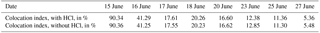
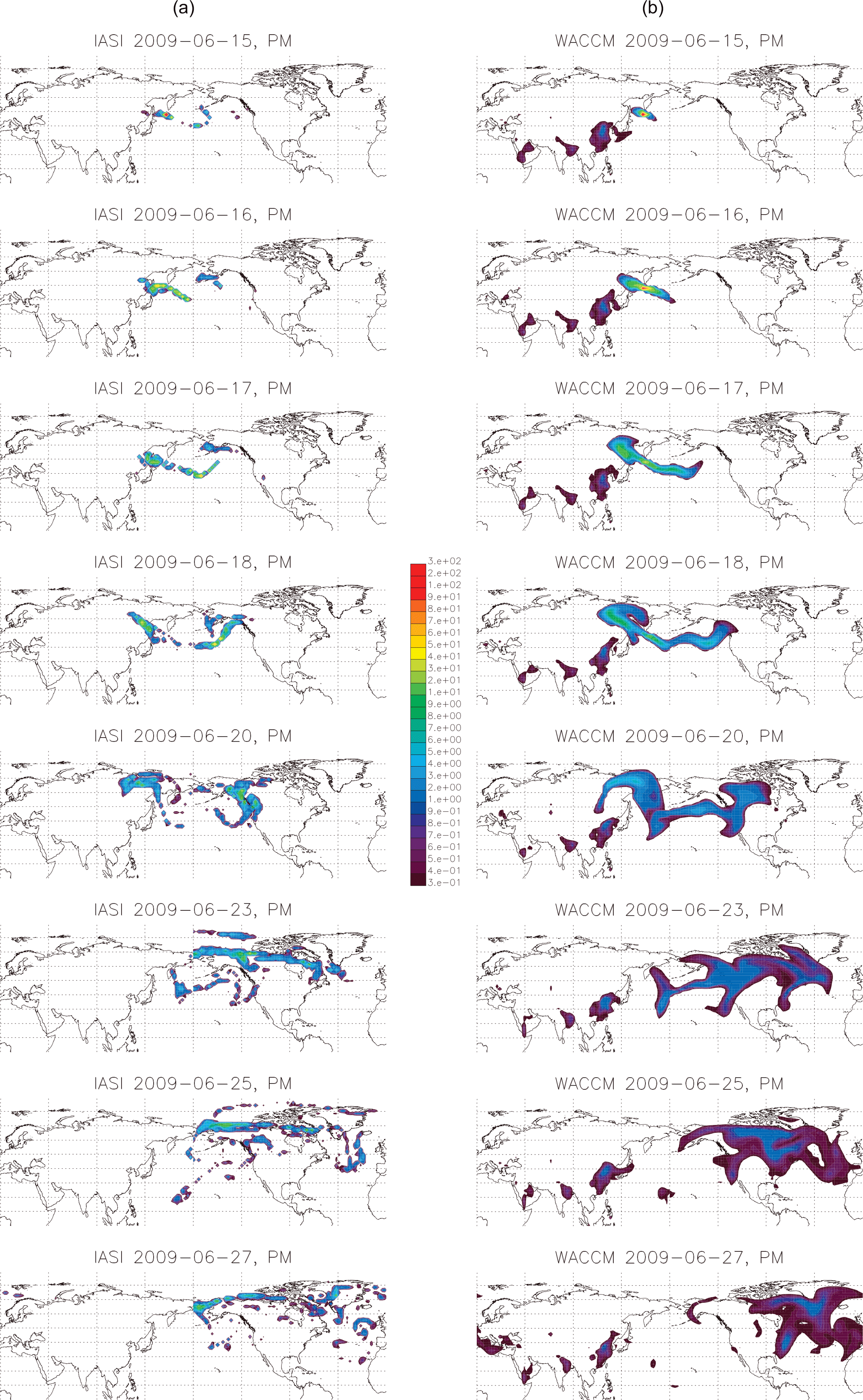
Figure 1 Spatial and temporal evolution of vertical column densities of SO₂ (in Dobson units, DU) over 1–2 weeks following the Sarychev eruption according to IASI satellite observations (a) and simulated by the CESM1(WACCM) model (b). A threshold of 0.3 DU was applied, corresponding to the lower threshold for this precise IASI retrieval (Clarisse et al., 2012). The CESM1(WACCM) model data correspond to instantaneous output at midnight, whereas the IASI data are gathered over the whole of the post meridiem period.

3.2 Lifetime, burden of volcanic SO₂, and role of co-injected HCl

Figure 2 shows the modelled northern hemispheric SO₂ burden in teragrams, calculated by integrating the model anomalies from CESM1(WACCM) simulations with SO₂ injection only and with SO₂ and HCl co-injection (anomaly denotes a volcano-on simulation from which the volcano-off control run has been subtracted). Two adjusted CESM1(WACCM) model results are also presented that only include data over columns with >0.3 DU SO₂ to enable a better comparison to the IASI observations. Alongside is shown the observed evolution in northern hemispheric SO₂ burden derived from the IASI retrieval by Clarisse et al. (2012) (which has a lower threshold of around 0.3 DU; see Sect. 2.2). Finally, we also show the northern hemispheric SO₂ burden as simulated using the HadGEM2 model (Haywood et al., 2010) and the IASI retrieval reported in that same study, both of which estimated 1.2 Tg SO₂ injection in contrast to the revised IASI analysis (Clarisse et al., 2012) that yielded 0.9 Tg SO₂ used in our study.

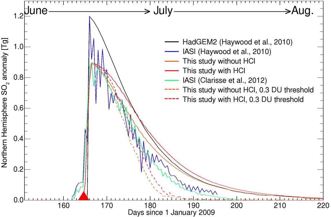
Figure 2 Temporal evolution of the SO₂ burden anomaly (in Tg), integrated over the Northern Hemisphere over June–August 2009. Model anomalies are shown for simulations that injected SO₂ only (orange) and with co-injection of HCl (red), alongside the IASI retrieval (green) with maximum burden of 0.9 Tg SO₂. Also shown are adjusted model outputs that account for the 0.3 DU IASI lower threshold for this particular case (red and orange dashed lines). For comparison, the previously reported model study and IASI retrieval of Haywood et al. (2010) that assumed a higher maximum burden of 1.2 Tg SO₂ are also depicted (black and blue lines, respectively).

A notable result is the slower decline in SO₂ burden for the model run with volcanic SO₂ and HCl co-injection than volcanic SO₂ (only). There is also a corresponding slower increase in the sulfate aerosol burden (Fig. 3).

The presence of HCl slows down the oxidation of SO₂ to sulfuric acid aerosol particles and hence lengthens the e-folding time of SO₂ in the stratosphere by about 2 days (see calculations below). This occurs as a result of the competition between their two main oxidation reactions involving OH. These are

$$\begin{array}{}\text{(R1)}& \mathrm{HCl}+\mathrm{OH}\to \mathrm{Cl}+{\mathrm{H}}_{\mathrm{2}}\mathrm{O}\end{array}$$

and the trimolecular reaction (where M is a third body, e.g. N₂ or O₂)

$$\begin{array}{}\text{(R2)}& {\mathrm{SO}}_{\mathrm{2}}+\mathrm{OH}+M\to {\mathrm{HSO}}_{\mathrm{3}}+M,\end{array}$$

where HSO₃ subsequently leads to the formation of H₂SO₄ through the reaction sequence described by Weisenstein et al. (1997). This conversion of SO₂ to H₂SO₄ is limited by the rate of Reaction (1) below 40 km in altitude. Competition between Reactions (1) and (1) results in a slower rate of oxidation of volcanic SO₂ in the presence of co-injected HCl.

A second notable result is that all the unadjusted model outputs overestimate the SO₂ burden following the eruption compared to IASI measurements. The HadGEM2 model SO₂ exceeds the Haywood et al. (2010) IASI observations for the whole period. The unadjusted CESM1(WACCM) outputs also exceed the Clarisse et al. (2012) IASI observations after a few days. This behaviour contrasts with the two adjusted CESM1(WACCM) model outputs that correct for the 0.3 DU SO₂ lower value of the particular IASI retrievals used. The adjusted CESM1(WACCM) model outputs remain in close agreement with the observed post-eruption SO₂ burden for the first 1–2 weeks, after which the model-simulated SO₂ burdens decline more rapidly than the IASI 2012 observations. This evolution can be expected: a greater dispersion in the ${\mathrm{2}}^{\circ }\times {\mathrm{2}}^{\circ }$ model grid cells than in reality (and than observed by the IASI footprint of tens of kilometres) would cause an underestimation of the model SO₂ burden compared to IASI. This effect will become more pertinent with dilution over time as the SO₂ column approaches the 0.3 DU limit.

In summary, we find that the CESM1(WACCM) model run (adjusted output) with SO₂ and HCl co-injection gives the best agreement with the IASI SO₂ observations. The simulation with SO₂ with HCl injection therefore forms the basis for further analysis in Sect. 3.6.

Our model–observation comparison of SO₂ burden trends can also be quantified in terms of the e-folding time. The definition of the e-folding time τ is the following: let M(t) be the concentration of a species through time; if we assume it follows an exponential decay over a certain period of time t>t₀, then τ is such as $\forall t>t_{\mathrm{0}},M(t+\mathit{\tau })=M\left(t\right)/e$; i.e. τ corresponds to the time by which the concentration falls to 1∕e of its initial value. For these calculations, we choose the SO₂ burden maximum as the initial value (0.9 Tg in our study). The e-folding time constant for SO₂ is approximately 17.0 days for the simulation including HCl, about 2 days longer than the approximately 15.0 days for the simulation that was run without HCl. When these CESM1(WACCM) model outputs are adjusted to correct for the 0.3 DU SO₂ lower value of the particular IASI retrievals used, they yield e-folding time constants of 11.5 and 10.0 days, respectively. For the IASI SO₂ retrieval of Clarisse et al. (2012), we calculate 12.0 days, i.e. very similar to the adjusted model simulation with SO₂ and HCl co-injection (11.5 days). For comparison, Haywood et al. (2010) report that the HadGEM2 model yields a 13- to 14-day SO₂ e-folding time (assuming a higher SO₂ injection of 1.2 Tg and no HCl co-injection). Regarding IASI observations, Haywood et al. (2010) report an IASI SO₂ e-folding time of 10–11 days, whilst using our method we calculate 9.0 days for the IASI retrieval of 2010. This is summarized in Table 2.

Figure 3 Temporal evolution of total SO₂ and SO₄ burdens (Tg sulfur), integrated over the Northern Hemisphere over June–August 2009 (the eruption is depicted by the red triangle). Model anomalies are shown for runs with injection of SO₂ only (red and yellow for SO₂ and SO₄, respectively) and with co-injection of HCl (green and blue for SO₂ and SO₄, respectively).

Haywood et al. (2010)Haywood et al. (2010)

Table 2 Comparison of the calculated SO₂ e-folding times for this study and Haywood et al. (2010). Two sets of IASI data are investigated: 2010 and 2012 retrievals. For the sake of the comparison with the satellite data, a lower threshold of 0.3 DU is applied whenever possible. The most recent IASI data (2012) yield a value close to that calculated with the model simulation of this study with SO₂ and HCl co-injection. N/A indicates data that are not available.

Figure 4 Comparison of particle number concentration over Laramie (USA; 41^∘ N, 105^∘ W), simulated by the CESM1(WACCM) model (red/orange lines: simulations with and without the Sarychev eruption are shown as solid and dashed lines, respectively) and by balloon-borne in situ measurements (blue/cyan lines) for 22 June and 7 November 2009. Two size ranges are shown: d>20 nm (CN) and d>0.5 µm (N). The model tropopause height is depicted by the dashed grey line. Model uncertainties are greater in the troposphere. On 22 June 2009, the presence of a volcanic plume over Laramie is simulated in the model (evident in both CN and N at the tropopause; discussed in the text) but not evident in the observations. On 7 November 2009, the presence of a more dilute volcanic plume is simulated in the model (evident in N only) that is consistent with the observed N in the lower stratosphere.

3.3 Comparison of the model to in situ balloon-based measurements of size-resolved aerosol

Here, we compare size-resolved aerosol concentrations from our simulations with in situ measurements from balloon-borne OPCs over Laramie, USA (June and November 2009), and Kiruna, Sweden (August and September 2009). It should be emphasized that the instruments are likely to detect a wider range of particles and particle compositions present in the stratosphere, i.e. internally and externally mixed particles with some organic and meteoric components (Murphy et al., 2014), whereas our model simulations provide pure sulfuric acid aerosol particles only. Nevertheless, these are expected to be the dominant source of aerosol in the lower stratosphere in the months following the Sarychev Peak 2009 eruption.

First, we compare the model to measurements carried out by the University of Wyoming OPC (Deshler et al., 2003) during balloon-borne flights over Laramie, Wyoming (USA, 41^∘ N, 105^∘ W), on 22 June and 7 November 2009. These observations were made 1 week and nearly 5 months after the Sarychev eruption, respectively. Kravitz et al. (2011) previously suggested that a significant volcanic influence can be seen in the data from 7 November but not on 22 June, based on comparison with balloon flights from other years. Here, we compare the data directly to aerosol simulated by our model runs.

Figure 4 shows both the model and measured aerosol particle number concentrations over Laramie for two particle size ranges: d>20 nm (noted CN, for condensation nuclei) and d>0.5 µm (noted N). Overall, there is good general agreement between simulated and measured values in terms of number concentrations and in the general trend with respect to altitude and size range separation. Note that model–measurement differences are greater in the troposphere since only sulfuric acid particles are simulated.

The upper panel of Fig. 4 (22 June 2009) shows that the volcano-off simulation reproduces the in situ observations of particle number with a very good agreement, supporting the hypothesis of Kravitz et al. (2011) that there was no significant volcanic influence on this day. However, the volcano-on simulation in fact simulates the presence of a volcanic plume, as can be seen by enhancements in CN and N between 13 and 15 km altitude. We note that the precise geographical location of plume structures is difficult to simulate using low-resolution simulations just 1 week after the eruption. Remote sensing observations suggest the initial presence of multiple aerosol layers in the stratosphere that subsequently collapsed into a single layer (O'Neill et al., 2012), whereas our CESM1(WACCM) model study assumes injection over 11–15 km. We also suggest that model horizontal resolution effects are a further possible source of error in the volcano-on simulation that might have led to anomalous sulfate plume structure over the measurement location. A geographic 2-D map of the vicinity of Laramie that shows model-simulated sulfuric acid aerosol particles at 13 km altitude (Fig. A1) show that the location of the measurements lies on the edge of an aerosol plume structure simulated by the model. Diffusion on the model grids ($\mathrm{2}{}^{\circ }\times \mathrm{2}{}^{\circ }$ resolution) or uncertainties in the initialization altitude could therefore lead to modelled plume structure over Laramie that is not evident in the observations.

Conversely, on 7 November, the volcanic plume is simulated to be much more homogeneous (and dilute), covering a larger area that encompasses Laramie. The lower panel of Fig. 4 shows modelled and observed aerosol particle number concentrations for 7 November 2009. For the d>0.5 µm size range (N), the agreement between the volcano-on simulation and the in situ measurements below 17 km indicates that volcanic aerosol particles were still present and detectable over Laramie nearly 5 months after the eruption, and their presence can be quantitatively reproduced by the CESM1(WACCM) model. The profiles from both volcano-on and volcano-off simulations are very close in the d>20 nm size range (CN) indicating the progressive return of the simulated concentrations to background conditions for this size range.

Next, we compare the CESM1(WACCM) simulations to in situ aerosol measurements made by the STAC instrument on a balloon gondola in northern Sweden. Figure 5 compares the particle counts observed by STAC and the sulfate particle concentrations simulated by the WACCM model for the same location (Kiruna, Sweden, 67^∘ N, 20^∘ E), and times: 2, 7, and 18 August 2009. A comparison is also shown for 18 May 2010 when the stratosphere can be considered to be close to background conditions. The model outputs have been interpolated to the pressure observed by the balloon payload and to the specific size bins of the STAC instrument covering 0.325 to 0.885 µm mean diameter.

In Fig. 5, a volcanic sulfate aerosol plume can clearly be identified between 11 and 19 km altitude for all flights in August 2009. This is demonstrated in the third column of the figure by an important difference in modelled particle number over the size bins of the STAC for the volcano-on and volcano-off simulations: total particle number on the STAC diameter range is enhanced by the volcanic eruption by between 1 and 2 orders of magnitude depending on the altitude. Total number simulated in the volcano-on simulation is in good general agreement with the STAC observations.

Figure 5 Comparison between STAC in situ measurements and CESM1(WACCM) simulations, over Kiruna, for 2, 7, and 18 August 2009 (plume detection), and 18 May 2010 (expected background conditions), and for altitudes ranging from 7 to 20 km. (a) Particle counts operated by STAC, separated in size bins between 0.325 and 0.885 µm diameter. (b) Simulated equivalent through the use of the CESM1(WACCM) model. (c) Comparison of the total particle counts for STAC and the model, over the STAC size range. The red dashed line shows results from the simulation without volcanic aerosols. Error on the STAC total counts can be evaluated to be ±6 %. The model tropopause altitude computed is represented by the horizontal black dashed line.

There are some discrepancies between model and observations at higher and lower altitudes: at lower altitudes, the model yields lower counts than the instrument's counts: this is likely due to the presence in the troposphere of non-sulfate aerosols unaccounted for by the model. For the discrepancies above the plume's altitude, the radiometer MicroRADIBAL (French acronym for Micro RADIomètre BALlon) (Brogniez et al., 2003; Renard et al., 2008), flown alongside STAC, identified the presence of some light-absorbing particles around 20 km altitude (Jégou et al., 2013): these might have affected the STAC measurements (STAC is designed for sulfate particle detection) and were also not included in the model. Their origin is still to be determined. Nevertheless, the good agreement in total number between model and observations in the lower stratosphere (corresponding to the main influence of the volcanic plume) confirms the strong impact of the Sarychev eruption on aerosol number.

Comparing these aerosol observations above Kiruna in August to those above Laramie in November on an order of magnitude basis, the Laramie measurements have ≈1 cm⁻³ particles of diameter greater than 0.5 µm at 14 km altitude in November, whereas measurements over Sweden in August of the same year show approximately 10 to 100 times more particles of size greater than 0.4 µm in diameter. This indicates the result of coagulation, condensation, sedimentation, and transport and dilution processes: 2 months after the eruption there is a strong volcanic impact, but few submicrometer-size volcanic particles are left in the stratosphere 5 months after the eruption. The volcanic aerosol evolution is discussed further in Sect. 3.5.

Figure 6 shows the particle size distributions measured by the STAC, separated in 1 km layers of altitude, for the same four flights as Fig. 5, and compares these to size distributions simulated by the CESM1(WACCM) model. The size distributions are displayed in terms of number, surface, and volume, and should be read by pairs, comparing the STAC observations to the control run (volcano-off) on the one hand, and the simulations including the volcano eruption (volcano-on) on the other hand.

The figure highlights that the control run underestimates the particle number (area or volume) size distribution curves by orders of magnitude compared to the STAC observations. A much better agreement is found when the volcanic emission is included in the model simulations, showing a good ability of the model to reproduce volcanic aerosol plumes in terms of aerosol size distribution. For 18 May 2010, nearly 1 year after the eruption, the difference between the volcano-on simulation and control run is much less noticeable. This comparison reflects the ability of the model to simulate stratospheric aerosol size distributions in background (or near-background) conditions.

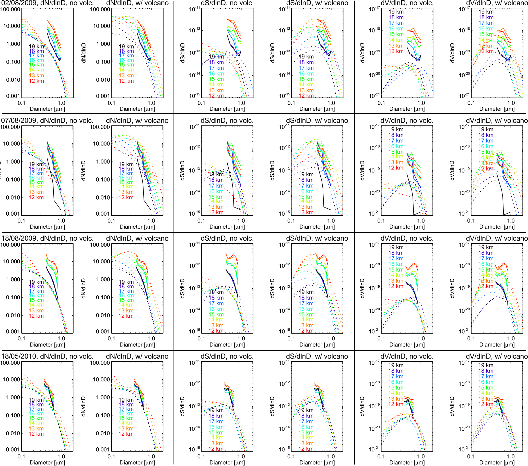
Figure 6 Particle size distributions in terms of number, area, and volume, separated for different altitude layers, shown for the same 4 days of interest already presented in Fig. 5. Size distributions observed by STAC are shown as solid lines and simulated by CESM1(WACCM) as dashed lines. Graphs go by adjacent pair: comparison of STAC data to both the volcano-off and the volcano-on cases highlights the improved agreement between model and measurements for simulations when the volcano is active. The measurement error on STAC measurements can be evaluated to be ±6 %.

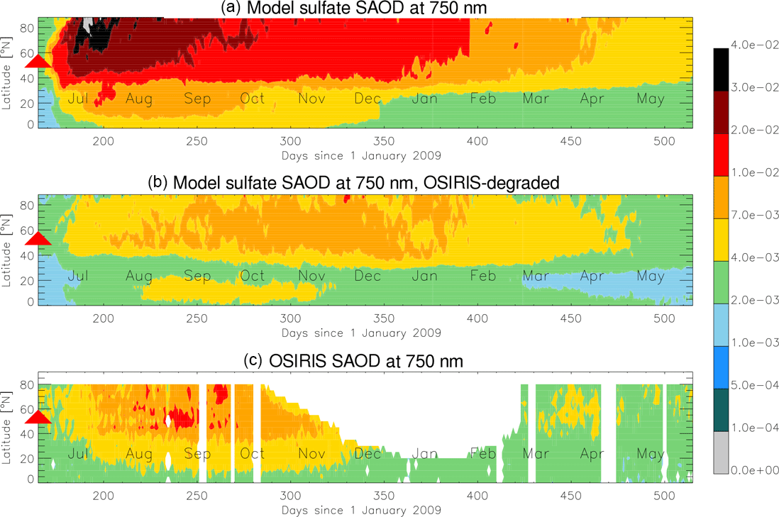
Figure 7 Comparison of modelled and observed stratospheric aerosol optical depth. (a) Stratospheric sulfate aerosol optical depth at 750 nm as simulated by CESM1(WACCM). (b) CESM1(WACCM)'s stratospheric sulfate AOD at 750 nm degraded to account for limitations in OSIRIS data (including saturation effect and minimum altitude). (c) Actual OSIRIS SAOD retrieval obtained from data with measurement limitations (see text for details).

3.4 Comparison of the model SAOD to OSIRIS observations

Extinction data from OSIRIS have been used for model and observational assessment of stratospheric aerosol impacts following the Sarychev 2009 eruption (Haywood et al., 2010; Jégou et al., 2013; Kravitz et al., 2011; O'Neill et al., 2012). However, as mentioned in the introduction, biases in the OSIRIS measurement following volcanic eruptions can affect the reported model–observation comparisons.

In Fromm et al. (2014), a detailed analysis of OSIRIS's limitations was carried out. These authors have shown that two main factors affect the derivation of SAOD by OSIRIS: (i) an upper detection limit on the value of extinctions, above which the measured values saturate, and (ii) a latitude dependence in the minimal altitude above which extinctions are integrated to yield the SAOD.

As pointed out by Fromm et al. (2014), it is impossible to reverse this process of data degradation; the best we can achieve to perform consistent model-to-observation comparisons is to degrade the extinctions derived from the model in order to derive SAOD “as OSIRIS would detect it”. It must nonetheless be emphasized that such a comparison is not a complete evaluation of the model performance: any agreement found cannot fully validate aspects of the model output that are removed in the degradation process. Nevertheless, such a comparison of the degraded model to (biased) satellite observations is highly valuable: it enables an assessment of model performance on a global scale, which cannot be achieved using local-scale in situ observations.

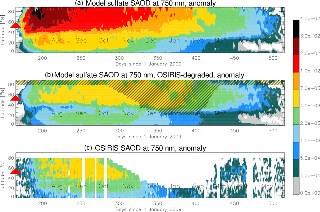
Figure 8 Comparison of modelled and observed anomalies in stratospheric aerosol optical depth. The absolute SAOD data from Fig. 7 have been converted to anomalies by subtracting modelled or observed SAOD 1 week before the eruption. (a) Stratospheric sulfate aerosol optical depth anomaly at 750 nm as simulated by CESM1(WACCM). (b) CESM1(WACCM)'s stratospheric sulfate SAOD anomaly at 750 nm degraded to account for limitations in OSIRIS data (including saturation effect and minimum altitude). (c) Actual anomaly in OSIRIS SAOD retrieval obtained from data with measurement limitations. The shaded area denotes the polar night, where OSIRIS's measurements are missing; see text for details.

We use the following method: first, we allow the extinctions calculated in the model to saturate, with an upper threshold of $\mathrm{2.5}\times {\mathrm{10}}^{-\mathrm{3}}$ km⁻¹ corresponding to the detection limit described in Fromm et al. (2014). Second, extinctions are integrated over truncated vertical columns of the atmosphere, introducing a lower altitude limit dependent on the latitude and the local tropopause height. Following Fromm et al. (2014), we define the minimal altitudes Z_min above which the extinctions are integrated as

$$\begin{array}{}\text{(2)}& Z_{\text{min}}(\mathit{\lambda },\mathit{\varphi },t)=Z_{\text{trop}}(\mathit{\lambda },\mathit{\varphi },t)+\mathrm{\Delta }\left(\mathit{\varphi }\right),\end{array}$$

where Z_trop is the local tropopause height, λ is longitude, ϕ is latitude, t is time, and Δ is a positive offset function, which was taken in our case as linearly varying with latitude from 0.5 km at the Equator to 5.5 km at the poles. These were chosen as a trade-off between the histogram of values in Fromm et al. (2014) and actual minimum altitudes reached by OSIRIS over the 2009–2010 period (see Appendix Fig. A2). For this series of calculations, thermal tropopause heights were diagnosed in the model. We verify the broad consistency of these altitude limits for OSIRIS data during the 2009–2010 Sarychev post-eruption period in Fig. A2. Integrating the model-simulated saturated extinctions at 750 nm over the truncated altitude columns as defined above gives SAOD values that can be considered reasonably consistent with the measurements performed by OSIRIS.

Figure 7a shows the zonally averaged stratospheric sulfate AOD, through time, over the Northern Hemisphere, as computed by CESM1(WACCM) in the volcano-on simulation (with co-injection of HCl). A degradation of the model data was then performed following the method described above. The resulting estimation of the sulfate SAOD “as would be detected by OSIRIS” is shown in Fig. 7b. Figure 7c shows the observed SAOD measured by OSIRIS. Over the winter months, there is a lack of observational data from mid-October 2009 until the beginning of 2010, particularly at high latitudes, that coincides with the polar night. A precise comparison for these months is therefore not possible. CESM1(WACCM) suggests that the sulfate SAOD remains at a fairly constant level over the Northern Hemisphere over the October–December 2009 period, then decreases quite quickly from February to April 2010.

The degraded model SAOD shows reasonable agreement with the SAOD observed by OSIRIS, whilst the non-degraded model simulates much higher SAOD. This demonstrates that OSIRIS's limitations are crucial to the interpretation of its data. In Fig. 7, the observed (OSIRIS) SAOD shows, however, a slightly stronger maximal magnitude than the degraded SAOD from the model. A possible explanation may be that CESM1(WACCM) yields extinctions for sulfuric acid particulates only, whereas OSIRIS's observations account for a more comprehensive SAOD that can include non-sulfate compounds in the lower stratosphere.

To place a greater emphasis on sulfuric acid particulates due to the volcanic eruption, we convert all three data sets to anomalies. These anomalies were calculated by subtracting background conditions from the SAODs, for which averages calculated in the first week of June 2009 were used as an approximate reference. Figure 8 presents the same layout as Fig. 7 but now displays the SAOD anomalies over the same period (1 June 2009 until 31 May 2010). Again, a good accordance is found between the degraded model compared to OSIRIS (with the non-degraded model showing higher SAODs). The agreement in SAOD anomalies in Fig. 8 is better than for the absolute SAODs in Fig. 7. This indicates that differences in the background aerosol content prior to the eruption may explain some of the model–measurement discrepancy in terms of SAOD maximum amplitude as highlighted in Fig. 7.

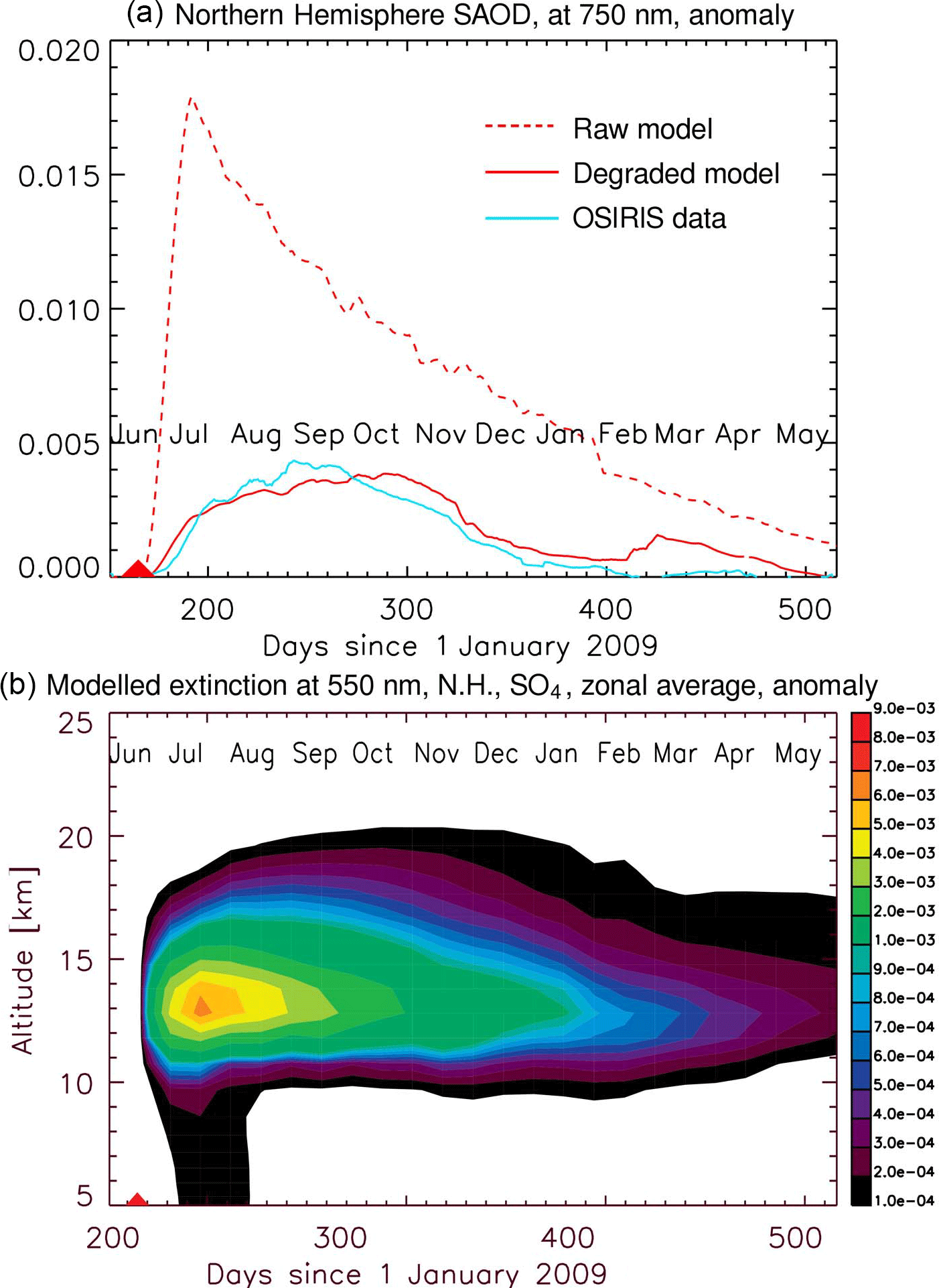
Figure 9 (a) Northern Hemisphere SAOD anomalies at 750 nm calculated by integrating the model-simulated extinction (dashed red line), then degraded (full red line), and comparison with OSIRIS's actual data (blue line). The Sarychev eruption is symbolized by the red triangle. (b) Modelled temporal evolution of the sulfuric acid aerosol extinction coefficient at 550 nm, zonally averaged for the Northern Hemisphere, is displayed in anomaly (volcano-on minus volcano-off).

Integrating anomaly data presented in Fig. 8 yields the Northern Hemisphere SAOD anomaly calculated at 750 nm over the year following the eruption, shown in Fig. 9. The dashed red line is SAOD simulated by the model. The plain red line indicates the same data after the OSIRIS bias degradation, and the blue line indicates SAOD from OSIRIS observations. Note that missing data in OSIRIS's measurements during winter were taken into account in the integration of the degraded model data, as shown by the shaded area in Fig. 8. Figure 8 along with Fig. 9 point out very clearly that taking into account OSIRIS's limitations gives a very good match between simulated and measured AOD values. Figure 9b shows the modelled temporal evolution in 550 nm extinction coefficients, zonally averaged for the Northern Hemisphere, again highlighting maximum aerosol content around mid-July 2009.

Comparing the direct output of the model to OSIRIS in both Figs. 8 and 9 highlights a much stronger and faster formation of sulfuric acid aerosols in the model than can be detected by the OSIRIS instrument, which experiences strongest measurement biases shortly after the eruption due to the saturation effect. Further quantification is given below, including e-folding times.

Analysing the temporal evolution of the (non-degraded) model SAOD identifies a peak in the Northern Hemisphere 750 nm SAOD of ≈0.018 on 12 July 2009 (Fig. 9), followed by a long decay with an e-folding time of ≈169 days. Conversely, OSIRIS shows a much fainter and later peak (≈0.004 on 1 September 2009), with a quicker decay (e-folding time of 52 days). The degraded model SAOD yields an e-folding decay time (51 days) that is very comparable to that from OSIRIS; the peak value is also similar in amplitude to OSIRIS's and is reached on 17 October. This is slightly later than in the OSIRIS data, although the plateau in SAOD during that period can account for this delay.

Haywood et al. (2010)Kravitz et al. (2011)

Table 3 SAOD e-folding times calculated for the model simulations and for OSIRIS's data reported in previous publications (Haywood et al., 2010; Kravitz et al., 2011) and in the present study. Different latitude bands are considered, and the decay times are all calculated considering SAOD values.

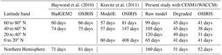
Table 3 summarizes the SAOD e-folding times calculated in this study, along with values from previous studies (Haywood et al., 2010; Kravitz et al., 2011), and calculated using OSIRIS data. Different bands of latitude are explored. One can note that the e-folding times vary quite significantly between authors, including those computed from OSIRIS's data (it is likely that different versions of the OSIRIS data – v.5.05 up to v.5.07 for the present study – were used). The main point to be highlighted here is the fair consistency obtained between e-folding times computed on the CESM1(WACCM)'s degraded data and on OSIRIS retrievals in our study, as evident from the last two columns of Table 3. We find that both the saturation limit and the fact that extinction profiles may terminate well above the tropopause are significant sources of measurement bias that need to be taken into account in comparison of OSIRIS data to model studies.

Figure 10 Zonally averaged effective radius simulated by CESM1(WACCM) model, in µm, as a function of altitude for three latitude bands (20 to 40, 40 to 60, and 60 to 80^∘ N). The model tropopause is shown as a dashed line.

3.5 Post-eruption effective radius simulated using a sectional aerosol scheme

Discrepancies in the magnitude and e-folding times between model and OSIRIS SAODs have been previously mentioned (e.g. Haywood et al. (2010); Kravitz et al. (2011); O'Neill et al. (2012)) and are summarized here in Table 3. This led to a consequent questioning of the models' reliability to simulate sulfuric acid particle formation accurately in terms of timing, thought to be caused by the absence of nucleation of new particles in the model (Haywood et al., 2010; Jégou et al., 2013). Conversely, our study using the CESM1(WACCM) model, whose aerosol microphysics includes nucleation, finds very good agreement with OSIRIS retrievals of SAOD in terms of magnitude and temporally when the model SAOD is degraded to account for both saturation and minimum altitude limitations on the SAOD derived from OSIRIS measurements. The maximum in our (non-degraded) model SAOD is significantly higher (by a factor of ≈4.5) than estimated by both OSIRIS and earlier modelling studies of the 2009 Sarychev Peak eruption (Haywood et al., 2010). A key unconstrained parameter in these earlier studies was the stratospheric particle size distribution that exerts a strong influence on SAOD. It was set to yield an effective radius of around r_eff=0.13–0.15 µm in Haywood et al. (2010), with the model results from Kravitz et al. (2011) also adjusted to represent this size. Previous studies suggested higher r_eff for large-magnitude eruptions that injected SO₂ higher into the stratosphere (yielding longer-lived sulfate clouds): Russell et al. (1993) derived r_eff of 0.22±0.06 µm around 1 month after the Mt. Pinatubo 1991 eruption, whilst Stothers (1997, 2001) suggest post-eruption r_eff grew from around 0.2–0.3 to 0.4–0.5 µm over the timescale of 1 year. Conversely, a lower r_eff was thought to be reasonable for the moderate-magnitude 2009 Sarychev Peak eruption that injected into the lower stratosphere (yielding relatively fresh and shorter lived sulfate cloud), and appeared consistent with ground-based remote sensing at Mauna Loa (Hawaii, USA) (Barnes and Hofmann, 2001; Haywood et al., 2010).

Here, the sectional aerosol representation with full aerosol microphysics in CESM1(WACCM) enables to freely simulate the post-eruption evolution in particle size, without any a priori assumptions. Sulfuric acid is first produced by the oxidation of volcanic SO₂, which leads to formation of new sulfuric acid particles by nucleation. Processes such as particle coagulation and condensation of sulfuric acid onto the existing particles causes particle growth. Particles are removed from the stratosphere by sedimentation and tropopause folding (Hamill et al., 1997). The balance between these processes determines the overall size distribution and its effective radius. Figure 10 shows the zonally averaged effective radius simulated by the model for three latitude bands (20 to 40, 40 to 60, and 60 to 80^∘ N). Particle growth occurs in regions with elevated sulfate concentrations following the volcanic eruption (Fig. A3, Appendix). Particle size grows to reach a maximum in zonal mean r_eff of up to 0.2 µm in the lower stratosphere. The greatest enhancement in r_eff occurs at high latitudes as expected given the poleward atmospheric transport in the stratosphere. At midlatitudes, a temporary decrease in r_eff can also be seen immediately following the eruption: this is due to new particle formation (nucleation) of particles of a few nanometres' size. The latitudinal trend in r_eff simulated by our model is broadly consistent with the trend reported from ground-based remote sensing at Eureka (Nunavut, Canada) that found r_eff=0.29 µm (O'Neill et al., 2012), and with ACE measurements, which report r_eff=0.1–0.3 µm (Doeringer et al., 2012). Modelled absolute values of r_eff are also globally consistent with balloon-borne observations in August 2009 (Jégou et al., 2013). Aerosol size or r_eff exerts a strong influence on SAOD (Haywood et al., 2010). A priori assumptions in stratospheric particle size are thus a major source of uncertainty in model studies that do not freely simulate the aerosol size evolution, and that will tend to cause an underestimation of SAOD in cases where the assumed r_eff is lower than reality.

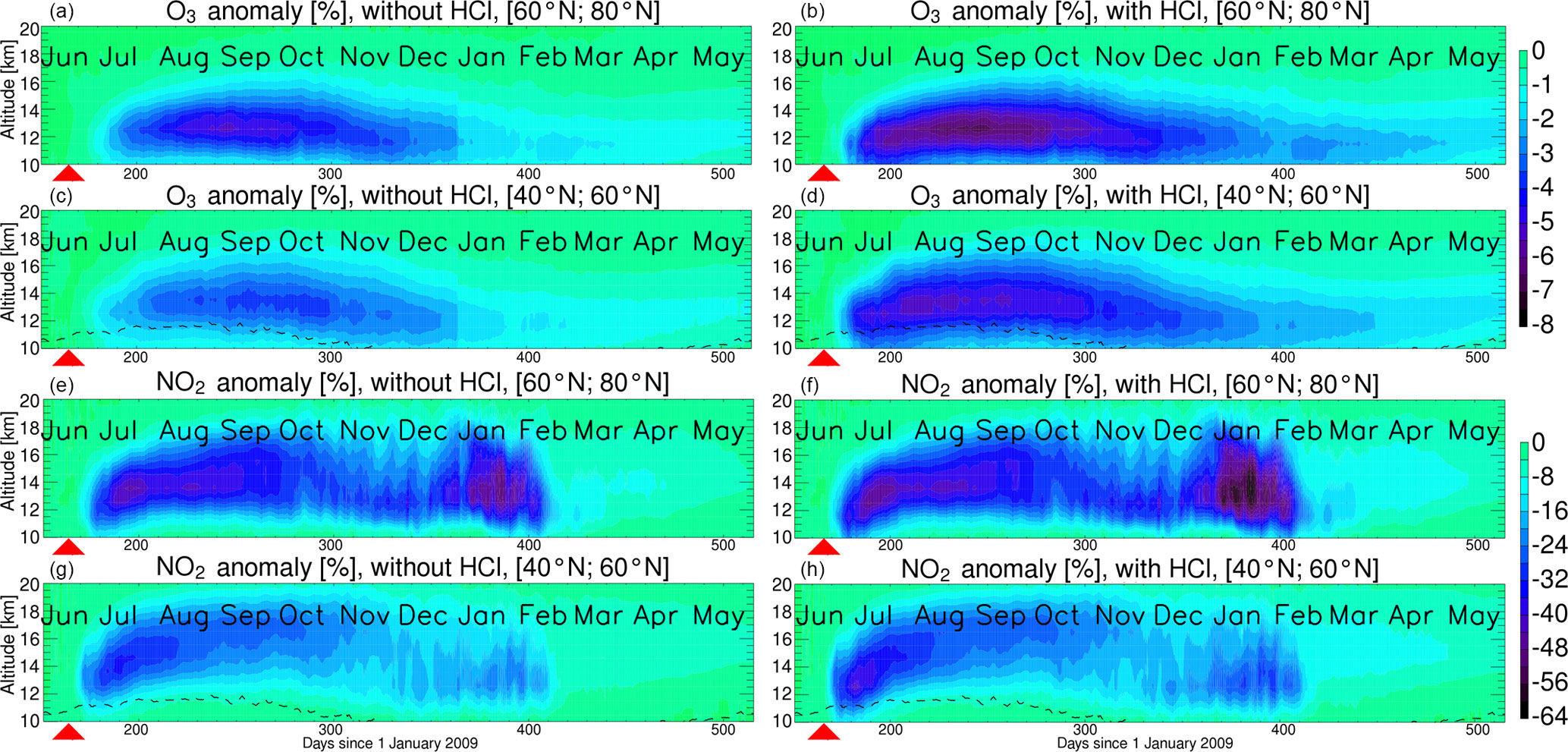
Figure 11 Zonally averaged depletions in stratospheric ozone and NO₂ at midlatitudes (40 to 60^∘ N) and high latitudes (60 to 80^∘ N) following the Sarychev eruption. Ozone is shown in the upper set of plots, NO₂ in the lower sets; within each pair, the latitudes are shown as 60 to 80^∘ N (upper plot of the pair) and 40 to 60^∘ N (lower plot of the pair). Simulations by the CESM1(WACCM) model are expressed as percentage anomalies (with respect to the volcano-off control run) and are calculated for the simulation with SO₂ injection only (a, c, e, g), and simulation with co-injection of HCl (b, d, f, h). Impacts on stratospheric chemistry are greater at higher latitudes and are enhanced by co-injection of volcanic HCl.

3.6 Effects of SO₂ and HCl co-injection on stratospheric chemistry

Most studies investigating the impacts of modern-day eruptions on stratospheric chemistry have focused on the role of sulfuric acid particles in reducing NO_x levels and activating pre-existing chlorine and bromine (ClO_x, BrO_x) in the stratosphere (Fahey et al., 1993; Solomon, 1999). One must note that halogens from the 1991 Mt. Pinatubo eruption were efficiently washed out and therefore did not reach the stratosphere (Mankin et al., 1992; Tabazadeh and Turco, 1993), though the washout for the Sarychev case was not necessarily as efficient (von Glasow et al., 2009). Observational evidence of stratospheric NO₂ depletion following moderate-magnitude volcanic eruptions is provided by Adams et al. (2017) based on satellite remote sensing, and Berthet et al. (2017) by balloon-borne observations following the Sarychev Peak eruption. Our study builds on these recent works in two aspects. First, we use the CESM1(WACCM) model with sectional aerosol representation. We freely simulate the aerosol surface area (SAD) (a function of particle number and size) that is a key control on stratospheric chemistry impacts. Second, we investigate the stratospheric chemistry influence of volcanic HCl that observations show was co-injected alongside SO₂ (Carn et al., 2016). The simulated anomalies in ozone and NO₂ for the latitudinal bands 40 to 60 and 60 to 80^∘ N are shown for simulations with SO₂ injection only, and for HCl co-injection with SO₂ in Fig. 11. In summer, greater depletions of up to −60 % for NO₂ are found at higher latitudes. This is primarily due to the higher aerosol loadings in these regions, and to favourable solar illumination conditions for which the catalytic ozone loss cycles (through OH radical production) are enhanced (Berthet et al., 2017). A more detailed description of the involved chemical processes is provided in Berthet et al. (2017).

Our results are broadly consistent with the observations of Adams et al. (2017), who reported that stratospheric NO₂ abundances were reduced by up to ≈45–55 % over 40–80^∘ N as consequence of the Sarychev eruption. Berthet et al. (2017) showed maximum NO₂ depletion of ≈50 % in the summertime lower stratosphere above Kiruna (Sweden) following the Sarychev eruption, based on REPROBUS model simulations with SAD prescribed from observations and without HCl injection. They predicted that ozone depletion reached up to 4 % in the lowermost stratosphere in summertime/early fall. Our CESM1(WACCM) simulation with a sectional aerosol scheme and injection of volcanic SO₂ (only) finds similar high-latitude maximum NO₂ reduction (≈50 %) and maximum ozone depletion (5 %). Interestingly, our simulations suggest somewhat greater maximum depletions in the simulation with co-injected volcanic HCl (7 and 60 %, for ozone and NO₂, respectively) compared to the simulation with SO₂ injection only (5 and 50 %, for ozone and NO₂, respectively). As a result of the enhanced stratospheric HCl budget throughout the season, more ozone-depleting chlorine radicals are expected to be formed due to Reaction (1) even at midlatitude conditions, though the impact on ozone appears limited. The impact on summer and fall NO₂ is negligible. In the polar winter, cold temperatures lead to further chlorine activation through heterogeneous processes enhancing some NO_x and ozone reduction. This study highlights the potential for volcanic HCl to complement and enhance SO₂–sulfate impacts on stratospheric chemistry, for eruptions where there is a significant HCl injection to high altitudes. The influence of Sarychev Peak eruption on stratospheric chemistry is nevertheless relatively modest, due to the moderate eruption size, in terms of both the SO₂ and HCl injected amounts.

4 Conclusions

We have presented a series of simulations carried out with the CESM1(WACCM) model for the study of stratospheric chemical impacts from the moderate-magnitude 2009 Sarychev eruption. Associated with the CARMA module, the model explicitly simulates the aerosol size evolution using a sectional aerosol scheme (across 30 size bins) and includes detailed aerosol microphysics. To simulate the eruption, we assumed a 0.9 Tg injection of sulfur dioxide between 11 and 15 km altitude over 1 day of eruption (15 June 2009). We also investigated the impacts of co-injected volcanic HCl.

Through comparison of the model results with satellite (IASI) retrievals of SO₂ and in situ measurements of stratospheric aerosols, we were able to assess the model performance, finding good agreement in terms of plume dispersion (Fig. 1) and particle formation rates (Figs. 2, 3), particle number concentrations as well as particle size distributions before and following the eruption (Figs. 4, 5, 6). In particular, very good agreement was found in terms of particle number concentrations and particle size distributions obtained from balloon-borne observations over Kiruna (northern Sweden) in July–August 2009 (Figs. 5, 6) and Laramie (Wyoming, USA) in November 2009 (Fig. 4), confirming the strong impact of the volcanic eruption on the stratospheric aerosol particle load. This suggests that particle formation is represented well in the sectional aerosol scheme (CARMA) in CESM1(WACCM). The simulations suggest that the effective radius (r_eff) becomes enhanced following the eruption reaching up to 0.2 µm in the zonal average. This is larger than the fixed aerosol size assumed in previous model studies with limited aerosol microphysics, e.g. r_eff=0.13–0.15 µm (Haywood et al., 2010).

The lack of more resolved data might be a source of uncertainty on the injection altitudes. However, this overall quantitative agreement reflects the model performance in SO₂ oxidation, atmospheric dispersion, and aerosol processing. It indicates a suitable choice of eruption source parameters as used in previous studies, e.g. Haywood et al. (2010) (an injection altitude ranging from 11 to 15 km for SO₂, a vertical even spread of the total mass of gases injected, and a sole injection of the total gas mass on 15 June 2009, neglecting other minor injections on other days). These eruption source parameters did provide good results. They might need to be refined for model studies at higher temporal or spatial resolution; see Günther et al. (2017); Wu et al. (2017). We point out that an injected mass of 0.9 Tg SO₂ (Clarisse et al., 2012; Realmuto and Berk, 2016) instead of 1.2 Tg of previous studies, e.g. Haywood et al. (2010), is a fair hypothesis, and enables the model to closely reproduce the observed SO₂ burden according to the IASI retrievals of Clarisse et al. (2012).

In addition, we investigated the co-injection of volcanic HCl to the stratosphere. Our simulations are based on the reported stratospheric HCl∕SO₂ mass ratio of 0.03 for Sarychev Peak eruption, according to analysis of satellite data by Carn et al. (2016). The altitude and timing of the HCl injection in the model were assumed to be identical to the SO₂ injection. Our study suggests that the presence of HCl leads to a delay in the oxidation of SO₂ to form sulfuric acid particles of about 2 days, with a 5–10 % increase in the modelled e-folding times for SO₂. We also find a better temporal accordance in SO₂ burden derived from satellite (IASI) data and our simulations when taking HCl into account. The additional surface area provided by volcanic particles catalyses reactions that can perturb stratospheric chemistry, including activation of stratospheric halogens, and can lead to strong reduction of NO₂ and modest depletion of ozone as highlighted by Berthet et al. (2017) for Sarychev Peak. Our simulations show that the co-injected volcanic HCl also affects the post-eruption stratospheric chemistry of ozone and NO_x, depleting these species more severely than in simulations that account for SO₂ injections only. Our results highlight that volcanic HCl emissions should be taken into account when simulating sulfur chemistry and stratospheric chemistry impacts from volcanic eruptions during which HCl is co-injected.

The second major point highlighted by this paper is the treatment of limitations in SAOD derived from OSIRIS measurements: both a saturation effect and a varying minimum altitude in available OSIRIS data (i.e. extinction profiles may terminate well above the tropopause, in particular at high latitudes) were identified by Fromm et al. (2014). We used a two-step model degradation process to reproduce these biases in the modelled data and found as a result very good agreement with the actual OSIRIS measurements following the volcanic eruption, reproducing both the magnitude and temporal evolution of the SAOD following the 2009 Sarychev eruption (Figs. 7, 8, 9, Table 3). Recent studies (Haywood et al., 2010; Kravitz et al., 2011; O'Neill et al., 2012) quantifying volcanic impacts tended to (only) incriminate their models' particle formation schemes because the comparisons with OSIRIS's satellite retrievals were poor specifically regarding the timing of the SAOD maximum. As a matter of fact, caveats on OSIRIS's measurement, as outlined by Fromm et al. (2014), are the key point to any model–observation comparison. We show that there is a considerably improved match between simulated and observed SAODs when these are taken into account. Once again, we stress that this agreement is only obtained by degrading the model output to account for OSIRIS's caveats; the fact that Figs. 8 and 9 show similar anomaly values cannot be sufficient to thoroughly validate the modelled SAODs through time. Rather, they provide supportive evidence to our study of stratospheric aerosol evolution following the Sarychev Peak 2009 eruption, using a model with detailed aerosol microphysics and sectional aerosol representation. The non-degraded output from our model shows substantially higher SAOD (maximum of 0.018 at 750 nm) than observed by OSIRIS (0.004), or as reported by previous model studies (with fixed aerosol size and limited microphysics). Our study therefore highlights that previous modelling studies (involving assumptions on particle size) that reported agreement with (biased) post-eruption estimates of SAOD derived from OSIRIS likely underestimated the climate impact of the 2009 Sarychev Peak eruption.

Appendix A

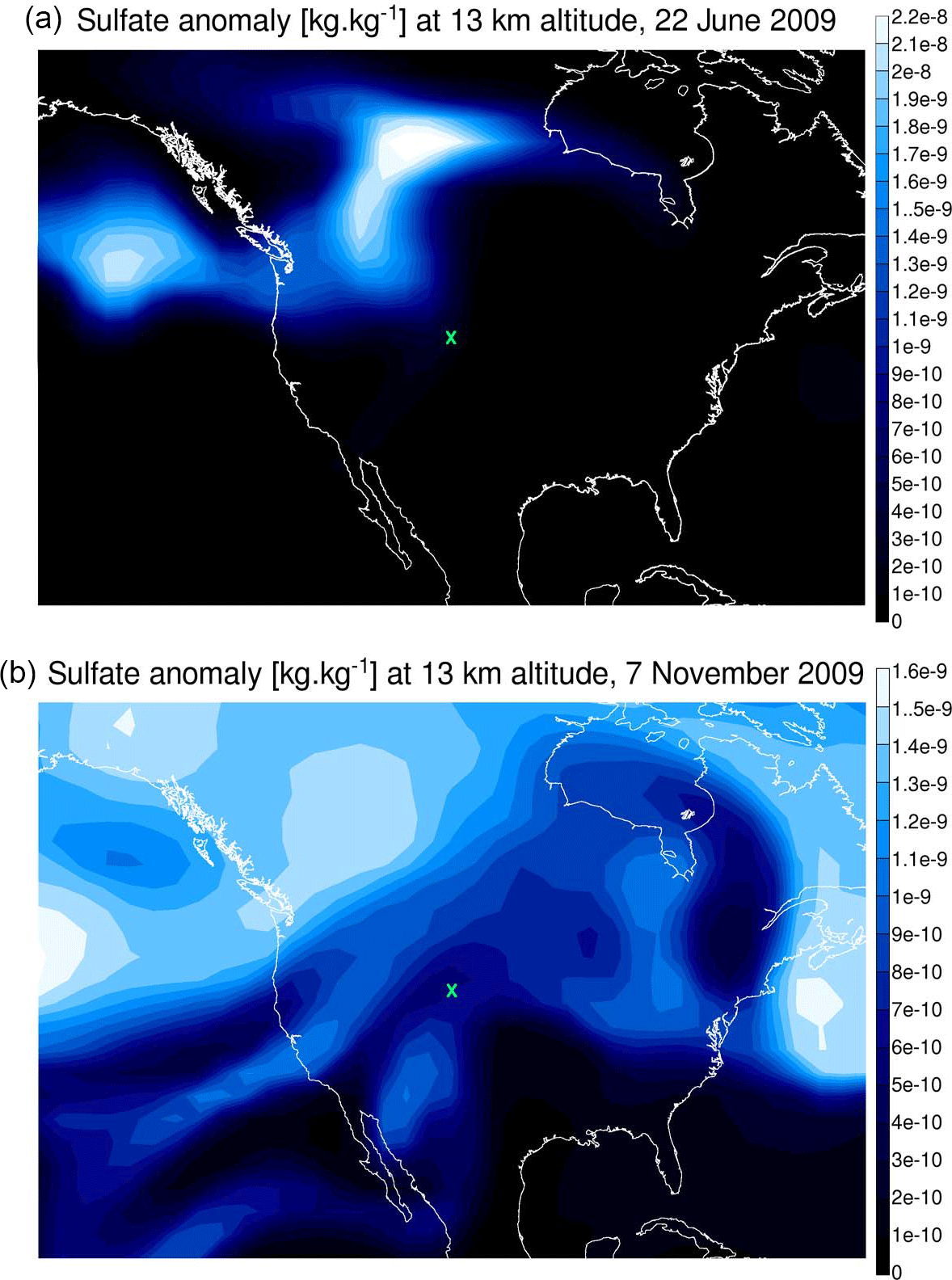
Figure A1 Geographic map over the USA displaying the simulated sulfate aerosol anomaly at 13 km altitude on 22 June 2009 (a) and 7 November 2009 (b), as computed by CESM1(WACCM). Note the order of magnitude difference in colour scale between the two plots. Laramie is indicated by the green cross: it is located on the very edge of a modelled aerosol plume structure on 22 June 2009 but below a more widespread (and dilute) plume on 7 November 2009.

Figure A2 Minimum altitude of OSIRIS extinction data calculated as an offset relative to the model tropopause as a function of latitude. OSIRIS data are shown for the first of every month from June 2009 to May 2010, with different colours depending on the month considered. There are some missing data during the winter in each hemisphere, particularly at high latitudes. The solid line shows the latitude dependence of the minimum altitude threshold assumed in the model degradation in this study.

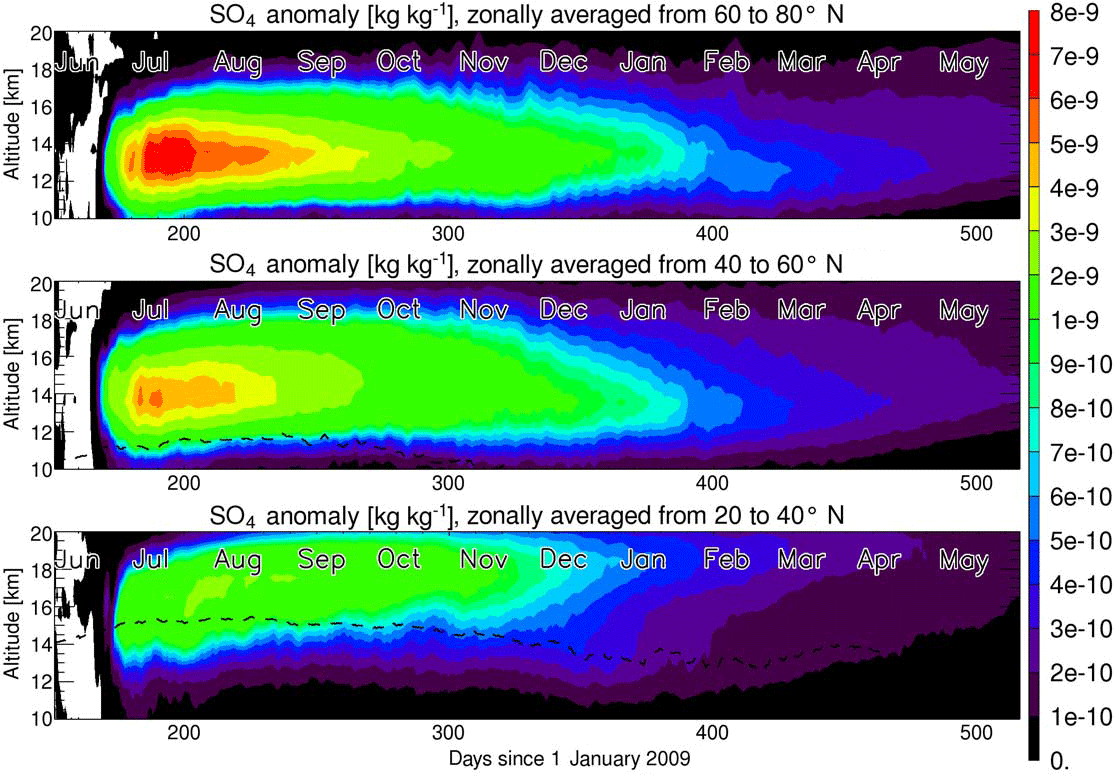
Figure A3 Zonally averaged sulfate anomaly, in kg kg⁻¹, as simulated by the CESM1(WACCM) model as a function of altitude for three latitude bands (20 to 40, 40 to 60, and 60 to 80^∘ N). The model tropopause is shown as a dashed line.