the Creative Commons Attribution 4.0 License.
the Creative Commons Attribution 4.0 License.
 | 06 Feb 2018
Simultaneous assimilation of ozone profiles from multiple UV-VIS satellite instruments
Jacob C. A. van Peet
Ronald J. van der A
Hennie M. Kelder
Pieternel F. Levelt
A three-dimensional global ozone distribution has been derived from assimilation of ozone profiles that were observed by satellites. By simultaneous assimilation of ozone profiles retrieved from the nadir looking satellite instruments Global Ozone Monitoring Experiment 2 (GOME-2) and Ozone Monitoring Instrument (OMI), which measure the atmosphere at different times of the day, the quality of the derived atmospheric ozone field has been improved. The assimilation is using an extended Kalman filter in which chemical transport model TM5 has been used for the forecast. The combined assimilation of both GOME-2 and OMI improves upon the assimilation results of a single sensor. The new assimilation system has been demonstrated by processing 4 years of data from 2008 to 2011. Validation of the assimilation output by comparison with sondes shows that biases vary between −5 and +10 % between the surface and 100 hPa. The biases for the combined assimilation vary between −3 and +3 % in the region between 100 and 10 hPa where GOME-2 and OMI are most sensitive. This is a strong improvement compared to direct retrievals of ozone profiles from satellite observations.
- Article
(3270 KB) - Full-text XML
- BibTeX
- EndNote


Depending on the altitude, ozone in the Earth's atmosphere has different effects. In the stratosphere, ozone filters the harmful ultraviolet part from the incoming solar radiation, preventing it from reaching the surface. Near to the surface, ozone is a pollutant, which has negative effects on human health and can reduce crop yields. At the same time, ozone is a greenhouse gas with an important role in the temperature of the atmosphere.
Because of the important role ozone has in climate change, it has been designated as an essential climate variable (ECV) by the Global Climate Observing System (GCOS) of the World Meteorological Organization (WMO, 2010). In the GCOS report, it is stressed that the full three-dimensional distribution of ozone is required.
The European Space Agency (ESA) has initiated the Climate Change Initiative (CCI) programme, which aims at long-term time series of satellite observations of the ECVs (http://cci.esa.int/). One of the sub-programmes is the Ozone CCI project (http://www.esa-ozone-cci.org/) that focuses on homogenized datasets of total ozone from different sensors (Lerot et al., 2014), stratospheric ozone distribution from limb and occultation observations (e.g. Sofieva et al., 2013), and the vertical ozone distribution from nadir observations (e.g. Miles et al., 2015). Long-term ozone datasets were also produced by the European Centre for Medium-Range Weather Forecasts (ECMWF) reanalyses such as ERA-40 (Uppala et al., 2005) and its successor ERA-Interim (Dee et al., 2011). Although primarily intended for improvement of the weather forecast, the assimilation of ozone is an integral part of theses reanalyses. ERA-40 is described in more detail in Dethof and Hólm (2004) and ERA-Interim in Dragani (2011). Total ozone column measurements from different satellite instruments were assimilated into a chemical transport model for the multi-sensor reanalysis (MSR) of ozone (van der A et al., 2010, 2015), spanning a 42-year period between 1970 and 2012.
Vertical ozone measurements from space-based ultraviolet (UV) instruments started with the Solar Backscatter Ultraviolet (SBUV) instruments from 1970 onwards on different satellites (e.g. Bhartia et al., 2013). Later, satellite instruments with higher resolution and increased spectral coverage were launched, for example Global Ozone Monitoring Experiment (GOME) onboard ERS-2 in 1995 (Burrows et al., 1999), SCanning Imaging Absorption spectroMeter for Atmospheric CHartographY (SCIAMACHY) onboard Envisat in 2002 (Bovensmann et al., 1999), Ozone Monitoring Instrument (OMI) onboard Aura in 2004 (Levelt et al., 2006) and Global Ozone Monitoring Experiment 2 (GOME-2) onboard Metop-A/B in 2006/2012 (Callies et al., 2000; Munro et al., 2016). Each location on Earth is typically observed once or twice a day by these satellites, so it is not possible to get global coverage at a specific time of the day. The retrieved ozone profiles from ultraviolet-visible (UV-VIS) nadir observations have a limited vertical resolution due to the smoothing effect in the retrieval (e.g. Rodgers, 1990). The vertical resolution varies between 7 and 15 km (see Hoogen et al., 1999). To derive gridded 3-D ozone distributions at fixed time intervals we use data assimilation, which combines the information present in the model and the observations, giving the optimal estimate of the ozone concentration. Either the retrieved ozone data or the radiance data from the instrument can be assimilated into the model. Migliorini (2012) showed that both methods are equivalent. However, assimilating retrieved ozone data considerably simplifies the observation operator and reduces the number of measurements to assimilate. Since the measurement, averaging kernel (AK) and error covariance matrices are all used in our assimilation algorithm, all information gained from the retrieval is also present in the resulting assimilated model fields.
Two commonly used types of data assimilation are 4DVAR and (ensemble) Kalman filtering. For example, ozone profiles and total columns from different instruments (such as GOME) were assimilated using a 4DVAR assimilation scheme in the production of the ECMWF ERA-Interim reanalysis (see Dragani, 2011). The Belgian Assimilation System for Chemical ObsErvations (BASCOE, http://bascoe.oma.be/; Errera et al., 2008) is a stratospheric 4DVAR data assimilation system for multiple chemical species including ozone and nitrogen dioxide. BASCOE is used in the Monitoring Atmospheric Composition and Climate (MACC) and Copernicus Atmosphere Monitoring Service (CAMS) projects for atmospheric services, the stratospheric ozone analyses from the MACC project are evaluated in Lefever et al. (2015). Recently, BASCOE has been coupled to the Integrated Forecast System of the ECMWF (Huijnen et al., 2016). 4DVAR is well suited to assimilate large amounts of observations, and the analysis provides a smooth field at the time of the assimilation. However, there are two disadvantages of 4DVAR with respect to Kalman filter techniques. First, 4DVAR requires the development and maintenance of an adjoint model, which is a complicated process. Second, 4DVAR does not produce a direct estimate of the uncertainty in the ozone field, although such an estimate can be derived using computationally expensive techniques.
The model covariance matrix is an integral and essential part of a Kalman filter, but it is difficult to derive and computationally expensive in the analysis calculation. Therefore, most Kalman filter implementations try to approximate the model covariance matrix. In the ensemble Kalman filter, a selection of the ensemble members can be used to approximate the model covariance (see Evensen, 2003; Houtekamer and Zhang, 2016). Miyazaki et al. (2012) used an ensemble Kalman filter to assimilate different trace gas measurements from multiple satellite instruments into a chemical transport model.
In this research, we follow the Kalman filter approach described in Segers et al. (2005), where the model covariance matrix is parameterized into a time-dependent standard deviation field and a time independent correlation field. The algorithm was updated and used by de Laat et al. (2009) to subtract the assimilated stratospheric ozone column from the total column in order to obtain the tropospheric ozone column. We have implemented several major updates and improvements in the algorithm compared to the version of de Laat et al. (2009). We check the observational error characterization, redefine the model error growth and derive a new correlation matrix for the ozone field. The new algorithm is the first that simultaneously assimilates nadir ozone profiles from multiple high-spectral-resolution satellite instruments. We demonstrate the new algorithm by assimilating ozone profile observations from GOME-2 and OMI for the period 2008–2011 into the chemical transport model TM5 (e.g. Krol et al., 2005). To minimize the bias between the two instruments, we developed a bias correction based on ozone sondes to be applied to the observations before assimilation. A bias correction based on total column measurements from ground stations was earlier used for the MSR of total ozone (van der A et al., 2015). Since we assimilate ozone profiles, we require an altitude dependent bias correction for which ozone soundings are selected.
In Sect. 2 we briefly describe the ozone profile observations, and in Sect. 3 the chemical transport model that we use for the data assimilation is described. Section 4 gives a short overview of the assimilation algorithm, Sect. 5 describes the improvements applied to the assimilation algorithm and the results will be shown in Sect. 6. In Sect. 7 we demonstrate the performance of the assimilation algorithm over the Tibetan Plateau. A discussion of the results is given in Sect. 8 and the conclusions are presented in Sect. 9.
Data from the UV-VIS satellite instruments GOME-2 and OMI are available for the last 10 years.
GOME-2 (Callies et al., 2000; Munro et al., 2016) was launched onboard Metop-A in 2006. The instrument measures the solar light reflected by the Earth's atmosphere between 250 and 790 nm. For the retrievals used in this research, the radiance measurements are binned in the cross-track and along-track directions such that the ground pixels measure approximately 160 km ×160 km. The ozone profiles for GOME-2 are retrieved with the OPERA retrieval algorithm, which is described in van Peet et al. (2014). We increased the number of layers in this study from 16 to 32 for more accurate radiative transfer model results.
OMI (Levelt et al., 2006) was launched onboard Aura in 2004. The instrument measures the solar light reflected by the Earth's atmosphere between 270 and 500 nm. One important difference between OMI and GOME-2 is that OMI does not use a scanning mirror like GOME-2, but a fixed 2-D CCD detector. One dimension of the detector is used to cover the spectral range, the other is used to cover the cross-track direction. The ground pixels for the profiles retrieved from the UV-VIS spectrum measure approximately 13 km ×48 km in nadir. Note that only 1 in 5 scan lines are retrieved. The size of the ground pixels is increasing towards the edge of the swath. OMI has two UV channels that are used in ozone profile retrieval: UV1 and UV2. UV1 has 30 cross-track pixels, while UV2 has 60 cross-track pixels. The UV2 pixels are therefore averaged to coincide with the UV1 pixels. A description of the OMI ozone retrieval algorithm and validation results with respect to ground measurements and other satellite instruments can be found in Kroon et al. (2011).
The algorithms used to retrieve the ozone profiles from GOME-2 and OMI are both based on an optimal estimation technique. The state of the atmosphere is given by the state vector x, while the measurement is given by the measurement vector y and error ϵ. These two vectors are related by the forward model F according to . Following the maximum a posteriori approach (Rodgers, 2000), the solution is given by
where is the retrieved state vector, xa is the a priori state of the atmosphere, A is the averaging kernel, xt is the “true” state of the atmosphere, G is the gain matrix (), Gϵ the retrieval noise, is the retrieved covariance matrix, I is the identity matrix, Sa is the a priori covariance matrix, K is the weighting function matrix or Jacobian (it gives the sensitivity of the forward model to the state vector) and Sϵ is the measurement covariance matrix.
The averaging kernel can also be written as and gives the sensitivity of the retrieval to the true state of the atmosphere. The trace of A gives the degrees of freedom for the signal (DFS). For the cloud-free retrievals over the ozone sonde stations used in this study, the mean DFS for GOME-2 is 5.0 and for OMI is 5.1. When the DFS is high, the retrieval has learned more from the measurement than in the case of a low DFS, when most of the information in the retrieval will depend on the a priori state. The total DFS can be regarded as the total number of independent pieces of information in the retrieved profile. The rows of A indicate how the true profile is smoothed out over the layers in the retrieval and are therefore also called smoothing functions. Ideally, the smoothing functions peak at the corresponding level and the half-width is a measure for the vertical resolution of the retrieval.
Because the sensitivity of the retrieval to the vertical ozone distribution is represented by the averaging kernel, it is important to include the averaging kernel in the assimilation algorithm. Together, the retrieved state vector, the averaging kernel and error covariance matrices represent all information gained from the retrieval (Migliorini, 2012).
The model used in the assimilation is a global chemistry transport model called TM5 (Tracer Model, version 5), see Krol et al. (2005) for an extended description. The (tropospheric) chemistry of TM5 has been evaluated in Huijnen et al. (2010) and included into the integrated forecasting system of the ECMWF (Flemming et al., 2015).
In the current model setup used for the assimilation of the ozone profiles, TM5 runs globally with grid cells of 3∘ longitude × 2∘ latitude, on 45 pressure levels. The pressure levels are a subset of the 91-level pressure grid from the ECMWF. The meteorological data used to drive the TM5 tracer transport are taken from the ECMWF operational analysis fields, produced on these 91 pressure levels.
Above 230 hPa, ozone chemistry is parameterized according to the equations described by Cariolle and Teyssèdre (2007), using the parameters of version 2.1. In the troposphere, the ozone concentrations are nudged towards the Fortuin and Kelder climatology (Fortuin and Kelder, 1998), with a relaxation time that increases from 0 days at 230 hPa to 14 days at 500 hPa and lower. No other trace gasses are modelled in this setup, which makes this version of TM5 fast and computationally cheap. Ozone concentrations are prevented from following the model equilibrium state too closely by the frequent confrontation of the model with the observations during the assimilation process.
The assimilation algorithm uses a Kalman filter, and is described in Segers et al. (2005). The state vector xi (i.e. the ozone distribution at time t=i) and the measurement vector yi (i.e. the retrieved profiles at time t=i) are given by
where M is the model that propagates the state vector in time. It has an associated uncertainty w, which is assumed to be normally distributed with zero mean and covariance matrix Q. The observation operator H, which includes the averaging kernel, gives the relation between x and y. The uncertainty in y is given by v, which is also assumed to have zero mean and covariance matrix R (which is identical to in the retrieval equations). In matrix notation, the propagation of the state vector and its covariance matrix (P) are given by
where xf and xa are the forecast and analysis state vectors, respectively, at time t=i, i.e. before and after assimilation of the observations. The observations are assimilated according to
where K is called the Kalman gain matrix, and the matrix H is the sensitivity of the observation operator with respect to the state.
The observation operator interpolates the model field to the observation location, converts the model units to the retrieval units and takes the smoothing of the satellite instruments into account by incorporating the averaging kernel. The model grid cells are (longitude × latitude), much larger than the satellite ground pixels and therefore no horizontal interpolation is needed. The model profile, expressed DU layer−1, is converted to the pressure levels of the retrieval grid by applying a simple linear interpolation in the 10log (hPa) domain. For example, if the L2 profile layer overlaps with three model layers for 20, 100 and 30 %, the interpolated model partial column is (where DUi is the partial column for layer i). Finally, the observation operator H is formed by applying the averaging kernel A to the difference between the state vector x and the a priori profile ya used in the retrieval:
with C being the unit conversion (from the models kg grid-cell−1 to the observations DU layer−1) and B being the vertical interpolation. The sensitivity matrix H used in Eqs. (9) and (10) is constructed as H=ABC.
In general, the number of elements in an ozone profile is much larger than the degrees of freedom (about 5 to 6). We can therefore reduce the number of data points per profile by taking the singular value decomposition of the A, and only retain the vectors with a singular value larger than 0.1 (this is an absolute threshold and not relative to the maximum singular value). The profiles and matrices are transformed accordingly.
The computational cost of the assimilation algorithm can be further reduced by minimizing the size of the model covariance matrix P. The TM5 model runs in the current setup on a horizontal grid of (latitude × longitude) on 44 layers, which makes the size of the covariance matrix (475 200)2 elements. A number of different approaches exist to minimize the size of the model covariance matrix. For example, in Eskes et al. (2003), the number of dimensions is reduced by only assimilating total columns, while the horizontal correlation depended only on the distance between the model grid cells. Here, we follow the approach described by Segers et al. (2005), by parameterizing the model covariance into a time-dependent standard deviation field and a constant correlation field. At each time step, the model's advection operator is applied to the standard deviation field. The error growth (i.e. the addition of Q in Eq. 7) is modelled by a simple mathematical function, more details can be found in Sect. 5.2. The model covariance matrix can now be calculated according to
with 𝔇(σ) being a matrix with the values of the standard deviation σ on the diagonal and C the correlation matrix. The correlation matrix is calculated differently than in Segers et al. (2005), more details can be found in Sect. 5.3.
Unfortunately, the matrix in the Kalman filter (Eq. 10) is badly conditioned, which makes the inversion sensitive to noise. Therefore, the eigenvalue decomposition of this matrix is calculated and the measurements are projected on the largest eigenvalues, which in total represent 98 % of the original trace of the matrix.
For the numerical stability of the assimilation algorithm, the difference between the observation and the model should not be too large. A filter is implemented that rejects the observation when the absolute difference between the observation and the model forecast is larger than 3 times the square root of the sum of the variance in the observation and the variance in the forecast:
with σy and the standard deviation of the observation y and the forecast H(xf) for layer i, respectively. Note that this is done on a layer-by-layer basis, i.e. if in one layer the difference is too large, the whole observed profile is discarded.
Not all available ozone profiles can be assimilated into TM5 because the computational cost would be too high. Averaging retrievals on the model grid (sometimes called superobservations) was not possible because the assimilation algorithm described in this paper requires AKs and averaging AKs is not straightforward. Therefore 1 out of 3 GOME-2 profiles and 1 out of 31 OMI profiles are used. These numbers are chosen such that more or less the same number of observations are assimilated for each instrument, taking into account the decrease in available pixels due to the row anomaly in OMI. For OMI, the outermost pixels on each side of the swath are neglected, because of the large area of these pixels. Of the resulting retrievals, only cloud-free scenes (cloud fraction ≤0.2) are assimilated in order to get the maximum amount of information from the troposphere.
The first version of our assimilation algorithm was described in Segers et al. (2005). They assimilated GOME ozone profiles for the year 2000. This dataset was extended to the period 1996–2001 by de Laat et al. (2009) who derived tropospheric ozone for this period. The assimilated GOME observations in the previous algorithm version had a pixel size of 960 km ×100 km, much larger than the pixels in the current research. Since 2009, the assimilation algorithm has been further developed and improved for use with GOME-2. The improved resolution of GOME-2 and OMI ozone profiles and improved retrievals offer new possibilities, but also require adaptations in the data assimilation. It is the first time that ozone profiles from two nadir looking instruments, GOME-2 and OMI, are assimilated simultaneously. This has resulted in a significant number of updates and improvements to the assimilation algorithm compared to the version described in Segers et al. (2005) and de Laat et al. (2009), which are outlined in the following sections.
5.1 Observational error characterization
The covariance matrix of the observations that is used in the assimilation is composed of two components, the error on the spectral observations and the error of the a priori information. Since the spectral errors affect the assimilation results, they are first verified using the following method.
For a given wavelength, two adjacent detector pixels may have a radiance or reflectance difference that depends on the slope of the spectrum. Given enough samples, the standard deviation of the mean difference is a good indication of the noise at that particular wavelength. The relative difference D is calculated as
where F is the radiance and λ1 the wavelength in detector pixel 1 and λ2 the wavelength in the adjacent pixel. Because the standard deviation is sensitive to outliers, a Gaussian distribution is fitted to the data. The fitted standard deviation is multiplied with the spectrum and compared to the reported noise in the level-1 data.
For GOME-2, we checked 4 days in 2008: 15 March, 25 June, 26 September and 25 December. On 10 December 2008 the band 1A/1B boundary was shifted from approximately 307 to 283 nm and the integration time in this wavelength range decreased from 1.5 to 0.1875 s as was already the case for the rest of band 1B. Therefore, the data for the first 3 days are combined, while the data for 25 December is treated separately. The analysis was performed for different subsets, such as latitude, solar zenith angle and viewing angle, but results are shown for latitude only.

Figure 1GOME-2 Metop-A radiance spectra calculated by OPERA: before (a) and after (b) the wavelength shift from 307 to 283 nm. The blue and red lines are the radiance and uncertainty that are used in OPERA. The green line shows the fitted standard deviations of the relative difference (see Eq. 14) multiplied by the radiance.
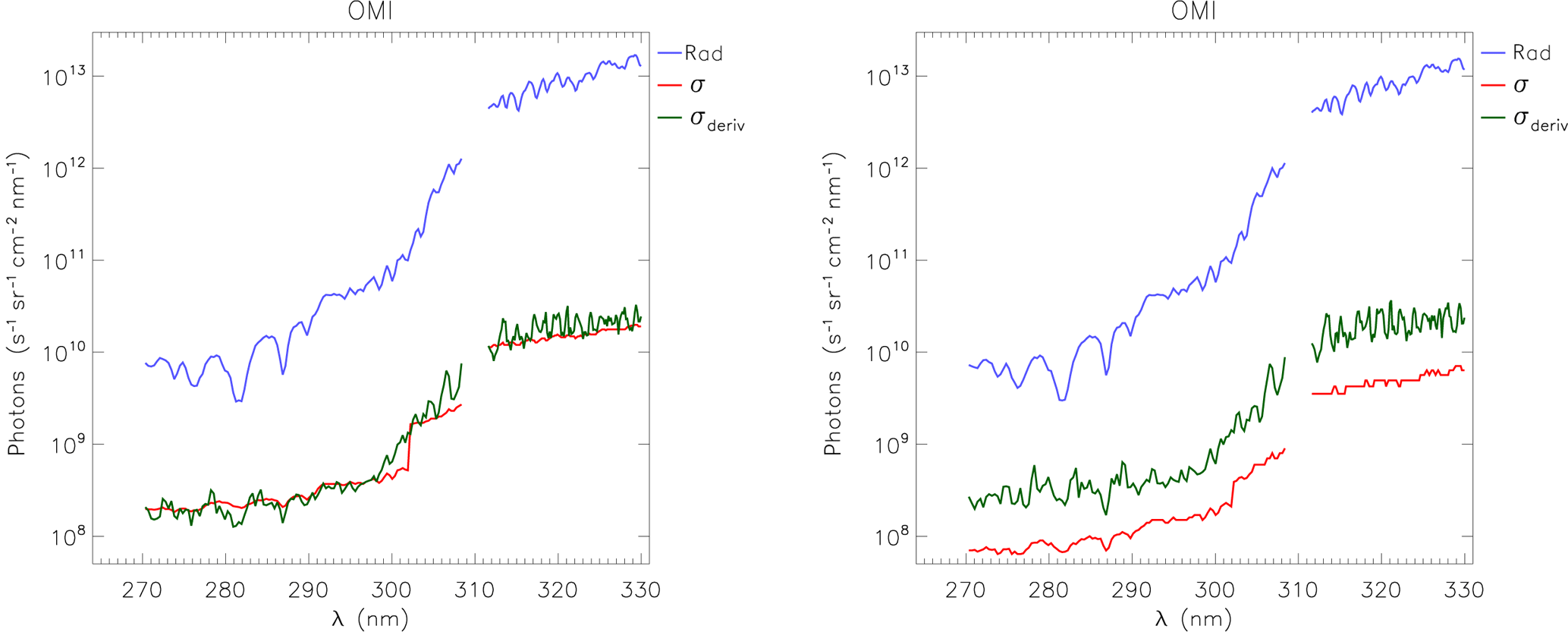
Figure 2OMI radiance spectrum used in the retrieval, the area around 310 nm is not used. The blue and red lines are the radiance and uncertainty, respectively. The green line shows the fitted standard deviations of the relative difference (see Eq. 14) multiplied by the radiance. Left plot before the L0 to L1b processor update: date = 25 February 2006, lon = 145.2∘, lat = ; right plot after the update: date = 5 February 2010, lon = 138.0∘, lat = .
Figure 1 shows the resulting GOME-2 radiance spectra for all wavelengths. It should be noted that the these results are made using spectral data derived from the GOME Data Processor (GDP) version 5.3. The older version GDP 4 uses a different noise model, which yielded too large errors.
The wavelength grid for OMI varies with the location across the detector, so the error verification has been performed with a dependence on the cross-track position. An example radiance spectrum along with the uncertainties is shown in the left panel of Fig. 2. There is a jump in the spectral uncertainty (the red line) around 300 nm, which might be related to a change in the gain settings for the detector. For the selected pixel, the gain changes with a factor of 10 at 300 nm.
On 1 February 2010, a L0 to L1b processor update was implemented for OMI. The new processor version includes more detailed information on the row anomaly and a new noise calculation for the three channels UV1, UV2 and VIS. More information can be found on the following website: http://projects.knmi.nl/omi/research/calibration/GDPS-History/GDPS_V113.html. The new noise calculation was investigated by taking the radiance differences determined a few days after the update. The resulting radiance spectra are given in the right panel of Fig. 2. The uncertainties in the L1 observations after the L0 to L1b processor update are about a factor of 5 smaller than the uncertainties derived according to the method described above.
In general, the spectral uncertainties for GOME-2 show a good agreement with our fitted uncertainties and therefore we simply use the uncertainties provided with the observations. The spectral uncertainties for OMI show a good agreement with our fitted uncertainties before the processor update, but are too small afterwards. The consequences of these smaller uncertainties will be shown in Sect. 6. Since we use the OMI observations as they are, we are not able to correct for the spectral uncertainties in the retrieval.
5.2 Model error growth
In Sect. 4 we explained that using the full covariance propagation from the Kalman filter equations is too computationally intensive. Instead we parameterize the model covariance matrix into a time-dependent standard deviation field and a time independent correlation field. The advection operator is applied to the standard deviation field, and the model error growth is modelled by applying a simple empirical relation.
In the previous version of the assimilation algorithm, the error growth for the total column was modelled by the function (Eskes et al., 2003), with A being a fit parameter. The error for the total column was distributed over the layers in the profile, proportional to the partial columns in each layer (Segers et al., 2005). Deriving a similar relation on a layer-by-layer basis was not successful, because the error can grow unlimited using this error growth description. Especially during the polar night, this might lead to unrealistic high error values.
Therefore, we use the following function
where a and b are parameters which can be determined by fitting the observation minus forecast root mean square (RMS) as a function of time (see Eskes et al., 2003, Fig. 2). The parameter a is the maximum error of the model at a particular altitude. At t=b, the error is 0.5a, therefore b is a measure of how fast the error grows after a measurement has been assimilated. The best results are obtained using b=2 (days) and let the value of a vary over altitude. The values of a are determined by comparing the free model run (i.e. no assimilation) with all sondes for 2008. Because the model currently runs on a (longitude × latitude) grid and the sonde observations are essentially point sources, these results include a representation error due to the grid-cell size of the model. The derived bias is therefore an overestimation of the real model error, and to prevent the model error from increasing too rapidly all collocations that are more than 3σ from the mean are discarded. The RMS values of the resulting collocations are used as values for a, they are shown as relative values in Fig. 3 for comparison over different altitudes. For the error of the layers above the maximum altitude of the sondes (about 5 hPa), a has been set to the same value as the last layer below the maximum altitude.
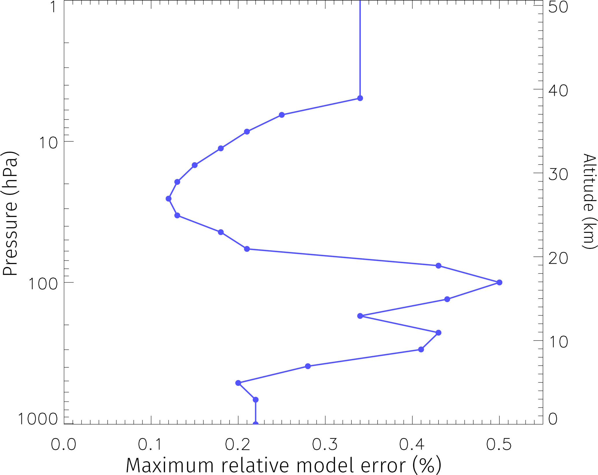
Figure 3Maximum relative model error (a) as a fraction of the partial column at different altitudes.
5.3 Model correlation matrix
In order to calculate the time independent correlation field, we follow the National Meteorological Center's method (NMC-method) to determine the correlation in the model (see Parrish and Derber, 1992; Segers et al., 2005). Segers et al. (2005) used a reference run based on 6-hourly meteorological forecasts as the starting point for forecast runs that last 9 days and start at 12:00 UTC. After a spin-up period, 9 forecast fields per day are available which can be used to determine the correlation in ozone. Differences between the ozone concentration in these runs are due to the different meteorological inputs. Since the overpass frequency of GOME is 3 days, the forecast field from the run started 3 days before the current date was used to derive the correlations in the ozone field. This choice also best matched the correlation length found by Eskes et al. (2003), where total columns were assimilated instead of profiles.
We use a slightly different approach as Segers et al. (2005) because their method neglects uncertainties due to the chemistry parameterization. Also, the forecast lag of 3 days is not compatible with GOME-2 and OMI, which have daily global coverage. Our reference run is the result of the assimilation of profile observations for April 2008, which we consider the true state of the atmosphere. Using the analysis field at 00:00 UTC, a model run without assimilation (a free model run) is started for a duration of 10 days. After the first 10 days, there are 11 model fields for a given date at 12:00 UTC: 1 from the assimilation run and 10 from the free model runs (see Fig. 4).

Figure 4Determination of the TM5 correlation field. The solid line is an assimilation model run, the dashed lines are 10 day free model runs. After 10 days, there are 11 ozone fields for each given day which can be used to determine the correlations.
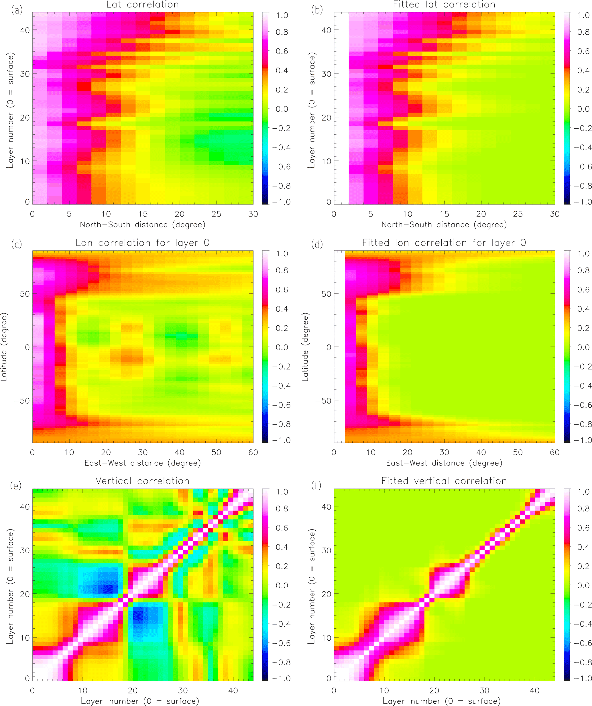
Figure 5Calculated (a, c, e) and fitted (b, d, f) correlations for the latitudinal (a, b), surface layer longitudinal (c, d) and vertical (e, f) directions.

Figure 6Global validation results for 2008–2011 for GOME-2 (a, b) and OMI (c, d). (a, c) show the median absolute differences, (b, d) show the median relative differences. The blue line indicates the original observations, the red line the bias corrected observations that have been used as input for the assimilation. The error bars indicate the range between the 25 and 75 % percentiles. Note that the x axis scale is different for each plot.
The difference between the assimilation and free model runs is used to determine the correlations between all pairs of grid cells in the vertical direction (constant location), in the East–West direction (constant latitude and altitude), and in the North–South direction (constant longitude and altitude). The correlations are determined as a function of the distance. Since the East–West distance between two grid cells is larger at the equator than near the poles, the East–West correlation also depends on the latitude. The calculated correlations as a function of distance are fitted with a Gaussian distribution (with correlations less than 0.01 set to zero). Both the calculated and fitted correlations are shown in Fig. 5. The fitted correlations are used in subsequent model runs as the time independent correlation field.
5.4 Ozone profile error characterization and bias correction
The biases between two instruments should be as small as possible for a stable assimilation. Therefore, a bias correction as a function of solar zenith angle (SZA), viewing angle (VA) and time has been developed based on the results of the comparison with sondes. The bias correction factor is one minus the median of the relative deviation based on all collocated data in a given year. All observations in a given year are multiplied by this correction factor.
Figure 6 shows the global validation results for the 4 years of the assimilation period (2008–2011) of the GOME-2 and OMI profiles with ozone sondes downloaded from the World Ozone and Ultraviolet Radiation Data Centre (WOUDC, WMO/GAW, 2016). The validation methodology has been described in van Peet et al. (2014), and the main characteristics are the following. Only cloud-free (cloud fraction <0.2) retrievals have been used, the sonde launch location should be located in the pixel footprint, and the satellite overpass time should be within 3 h of sonde launch. When multiple retrievals collocate with the same sonde, only the one closest in time has been used. The collocated sonde profiles have been interpolated on the pressure grid of the retrievals and extended to the top of the atmosphere with the a priori profile above the burst level of the sonde. The interpolated and extended profiles are convolved with the averaging kernels in order to take the vertical sensitivity of the satellite instruments into account.
Table 1Stations used for the validation and bias correction of GOME-2 and OMI.
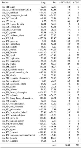
The bias of GOME-2 with respect to sondes varies between −1.1 and +1.7 DU (−7 and +7 %) between 100 and 10 hPa, while for altitudes below 100 hPa the bias is about −0.3 DU (−4 %). The bias of OMI varies between −4.5 and +2 DU (−8 and +15 %) between 100 and 10 hPa, while below 10 hPa the bias is positive with a maximum value of 4 DU (+27 %). The absolute biases cannot be compared directly because the layers of GOME-2 and OMI do not have the same thickness. Note that the remaining biases for the top layers in Fig. 6 are not exactly zero for the corrected observations, because the figure is drawn for latitude bands, while the bias correction is made using SZA and VA bins and the number of sondes used in the comparison at that altitude is much smaller than at lower altitudes. For the validation of GOME-2, 1083 sondes were used, of which 10 reached the top level. For the validation of OMI, 776 sondes were used, of which 33 reached the top level. Table 1 lists all stations and the number of sondes used in the validation and bias correction of the observations. The numbers in the station names refer to the WOUDC station identifiers.
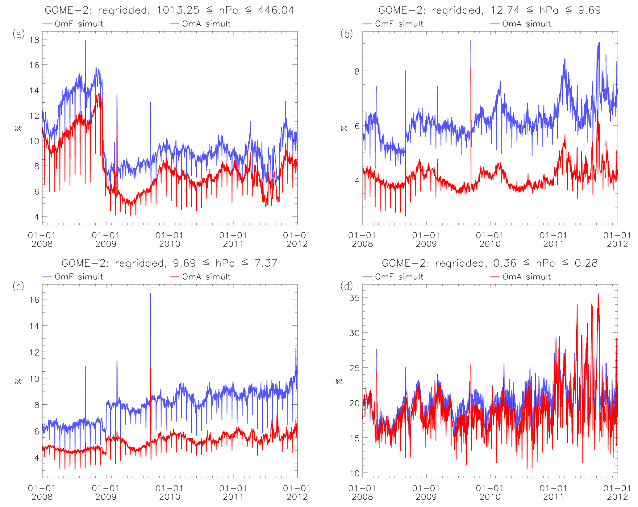
Figure 7GOME-2 OmF (blue) and OmA (red) for the surface layer (a), around 10 hPa (b and c) and around 0.3 hPa (d). The OmF and OmA have been calculated for the regridded layers from the model run with simultaneous assimilation of GOME-2 and OMI.
We have assimilated GOME-2 (on Metop-A) and OMI ozone profiles for a period of 4 years between 2008 and 2011 using the Kalman filter algorithm described in the previous sections. In total, four model runs were performed: a “free” model run without assimilation, a model run with assimilation of GOME-2 ozone profiles only, a model run with assimilation of OMI ozone profiles only and a model run with simultaneous assimilation of GOME-2 and OMI ozone profiles.
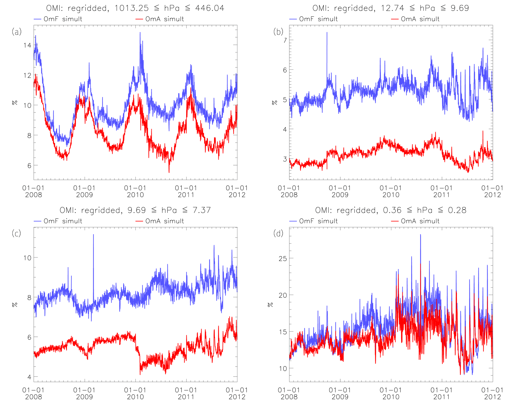
Figure 8OMI OmF (blue) and OmA (red) for the surface layer (a), around 10 hPa (b and c) and around 0.3 hPa (d). The OmF and OmA have been calculated for the regridded layers from the model run with simultaneous assimilation of GOME-2 and OMI.
6.1 Altitude dependent OmF and OmA statistics
An important diagnostic of any assimilation system is the difference between the observations and the model (also known as innovations). In the following, we define the relative observation minus forecast (OmF) for layer i as
with i the layer index, y the observed ozone profile, H the observation operator and xf the forecast profile of the model (see Sect. 4). The layers in the retrievals of GOME-2 and OMI have a different thickness, which makes the comparison of the OmF between the two instruments not straightforward. Therefore, both y and H(xf) have been regridded to the same pressure levels before calculating the OmF. This new vertical grid is defined by levels at 0, 6 and 12 km followed by levels every 2 up to 60 km, which are converted to hPa and correspond to surface pressure up to 0.28 hPa. The observation minus analysis (OmA) is defined in a similar way, but with xf replaced with the analysis profile xa. Since the analysis field is a weighted average of the forecast model field and the observations, the OmA should be smaller than the OmF.
In Fig. 7, the GOME-2 OmF and OmA from the model run with simultaneous assimilation of GOME-2 and OMI for four different layers have been plotted. The ozone sondes that were used in deriving the bias correction and the validation of the results were required to have reached at least 10 hPa. Therefore the selected layers in Fig. 7 are the surface layer, the layer just below and above 10 hPa, and the top layer of the new pressure grid around 60 km (0.3 hPa). In Fig. 8, the OmF and OmA for the same layers have been plotted for OMI. In the first year of the assimilation period, the surface layer OmF and OmA for GOME-2 are higher than those for OMI. At the end of 2008, after the wavelength shift between GOME-2 band 1A/1B, the situation is reversed and the OmF and OmA for GOME-2 are lower than those for OMI. The band 1A/1B wavelength shift is clearly present in the bottom layer of the GOME-2 OmF and OmA, which might be unexpected since the radiation from band 1A/1B does not reach the surface. But since the layers in an optimal estimation retrieval are related as described by the AK and covariance matrices, it is possible that the band 1A/1B change affects the results in an altitude region where the radiation itself does not penetrate. The OMI data show a more pronounced yearly cycle than GOME-2. After the beginning of 2010, the OmF and OmA for both instruments are very similar for the summer months June, July and August, but the winter time values for OMI are higher. For the layer just below 10 hPa, the OmF and OmA for GOME-2 are about 1 percentage point higher than for OMI. For the layer just above 10 hPa, the OmF and OmA for GOME-2 start out lower than for OMI, but at the end of the assimilation period the values are comparable. For the top layer, the OmF and OmA for GOME-2 are about 5 percentage points higher than for OMI. In general, the OmF is about 2–4 percentage points higher than the OmA, except for the top layer. There, the difference is in the order of 1 percent point, but the values vary much more than lower in the atmosphere.

Figure 9OMI OmF (blue) and OmA (red) for the layer around 0.3 hPa, zoomed in to a month before and after the L0 to L1b processor update. The OmF and OmA have been calculated for the regridded layers from the model run with simultaneous assimilation of GOME-2 and OMI.
Both OmF and OmA for the GOME-2 assimilation run show regular decreases with a period of about 1 month. These decreases are caused by GOME-2 being operated in “narrow-swath mode”, when the swath is 320 km wide instead of 1920 km. For these narrow-swath observations, the model is closer to the retrieved profiles, causing a lower OmF/OmA. OMI also has a spatial zoom-in mode, which is activated about once a month, but these pixels are filtered out because they are too much influenced by the row anomaly and because the mapping between the UV-1 and UV-2 pixels change with respect to the normal mode. Peaks in the OmF and OmA for the GOME-2 assimilation, such as after an instrument test period between 7 and 12 September 2009, can be related to periods of missing data.
Sudden changes in the OmF and OmA are visible for some altitudes for both instruments at the start of some years. One example is in the layer just above the 10 hPa for GOME-2 at the start of 2009 or at the start of 2010 for OMI. The change for GOME-2 appears to coincide with the band 1A/1B shift, but it is really at the start of the year and not on 10 December 2008. It is therefore unlikely that these two events are related. Since there are no known instrumental or meteorological changes, the most likely cause is therefore the bias correction scheme for the observations, which changes its correction parameters at the start of each year.
Closer inspection of the OMI OmF and OmA change at the start of 2010 (see the lower left panel of Fig. 8), shows that it actually consists of two steps: the first one at the start of the year and the second one a month later. That second step is also present in Fig. 8d (the layer around 0.3 hPa), where the change is about 5 percentage points, but it is less clear due to the higher variability in the signal. Figure 9 shows the same data, but focused on the first two months of 2010. Both OmF and OmA increase by about 5 percentage points from one day to the next. The increase is even larger (and more clearly visible) in the data from the single instrument assimilation run for OMI.
Comparison of Figs. 7 and 8 shows that the OmF and OmA for one instrument might be larger than for the other, depending on the altitude. Which of the two instruments has a larger OmF or OmA value might also change over time. In other words, GOME-2 and OMI have a different sensitivity for different altitudes as represented by the averaging kernels. Assimilating the observations from these instruments simultaneously increases the overall sensitivity of the assimilation.
Lower uncertainties in the spectra lead to lower uncertainties in the observations, which in its turn changes the balance between model and observations in the Kalman filter and affects the innovations. Because the variance in the observation is lower, more pixels will be rejected by the OmF filter (see Sect. 4 and Fig. 10). Figure 10 shows the number of assimilated observations for both GOME-2 and OMI from the single and simultaneous instrument assimilation. In the single instrument assimilation runs, the model error is adapted to the new situation after the processor update and the total number of assimilated observations does not change. For the simultaneous assimilation, the assimilation results may be fluctuating between OMI and GOME-2 observations if a bias exists. This might result in higher assimilation errors. Therefore, the OmF filter (see Sect. 4 and Eq. 13) rejects observations from both GOME-2 and OMI, even though only the uncertainties from one of the instruments (i.e. OMI) have changed.
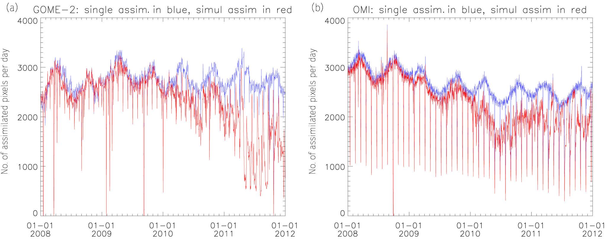
Figure 10Number of assimilated observations from GOME-2 (a) and OMI (b). The blue lines represent the single instrument assimilation, the red lines the simultaneous assimilation.

Figure 11Mean OmF (a) and OmA (b) as a function of latitude (bin size 2∘) and time (bin size 1 day) for the simultaneous assimilation of GOME-2 and OMI.
6.2 Altitude independent OmF and OmA statistics
In order to show the geographical distribution of the OmF and OmA, the absolute values for each layer were quadratically added and the square root was taken from the result. These column-integrated OmF and OmA values were averaged on a daily basis for latitude bins with a size of 2∘. In Fig. 11, these column-integrated OmF and OmA are shown as a function of latitude and time. The highest values of the OmF and OmA are observed at high latitudes around the polar night. The GOME-2 band 1A/1B wavelength change is clearly visible, even though the plot shows OmF and OmA from the combined assimilation. Step changes in the OmA are visible at the start of each year, which coincides with an update of the bias correction parameters.
6.3 Expected and observed OmF
The OmF of the results should be consistent with the uncertainties of the observations and the model forecast. The expected OmF is based on the observation error and the forecast error and is the mean of the square root term in the right-hand side of Eq. (13) for all observations in a given layer. The observed OmF for each layer for the whole assimilation period, on the other hand, is the mean of the left-hand side of Eq. (13). In Fig. 12, the observed OmF is plotted as a function of the expected OmF for the model runs with assimilation of GOME-2 only with assimilation of OMI only, and for both instruments separate with the data taken from the model run with simultaneous assimilation.

Figure 12Observed vs. expected OmF. (a) Assimilation of GOME-2 only, (b) assimilation of OMI only. (c, d) Results from the simultaneous assimilation of both GOME-2 and OMI. (c) GOME-2, (d) OMI. Colours indicate the pressure levels. Note that not all levels are plotted in the legend while all levels are plotted in the figure. The size of the circles gives the number of assimilated pixels (n) in that respective OmF-bin (bin-size =0.2 DU). The slope for the fitted (dashed) line is given in the lower right corner of each panel, as is the correlation (R) between the expected and observed OmF.
Note that the pressure levels are those from the observations, not the regridded levels used in the calculation of the OmF and OmA above. The expected and observed OmF are close to the 1-to-1 line, which shows that the model error is of the correct magnitude for the current observations. The expected and observed OmF are somewhat closer to the 1-to-1 line in the case of the simultaneous assimilation of GOME-2 and OMI than for the assimilation of each instrument independently. The model error that is used is therefore probably slightly better suited for the assimilation of multiple instruments simultaneously than for the assimilation of a single sensor.
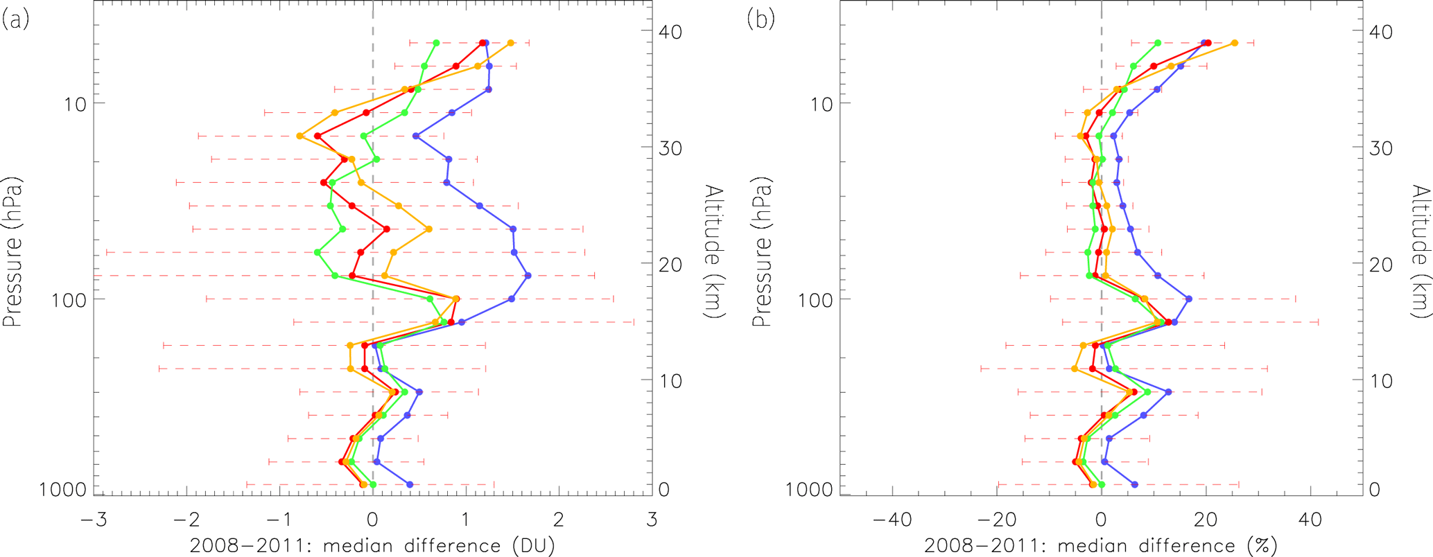
Figure 13Validation of the model runs with ozone sondes for 2008–2011. (a) The median of the absolute difference in DU, (b) the median of the relative differences. Blue: model run without assimilation, green: model run with assimilation of GOME-2 only, yellow: run with assimilation of OMI only, red: assimilation of both GOME-2 and OMI. The error bars are plotted for the simultaneous assimilation only, and range from the 25 to the 75 % percentile.
6.4 Assimilation validation with sondes
The model output was validated against ozone sondes that were obtained from the World Ozone and Ultraviolet Radiation Data Centre (WOUDC, WMO/GAW, 2016, see Fig. 13). This is the same ozone dataset as was used to derive the bias correction. Note, however, that many more observations are assimilated than were used deriving the bias correction, while all observations are corrected with the same factor. The assimilation model runs are significantly better than the free model run. This is especially true for the part of the atmosphere where GOME-2 and OMI are most sensitive to the ozone concentration, between 100 and 10 hPa. In this area, the model run with assimilation of GOME-2 only shows a negative bias with respect to the ozone sondes, while the assimilation of OMI shows a positive bias. The assimilation of both GOME-2 and OMI shows the smallest bias. The deviation in the differences are very similar for the four runs, which is why only the error bars for the simultaneous assimilation have been plotted in Fig. 13. The 25–75 percentile differences are in the 20–55 percentage points range between 0 and 20 km and in the 10–20 percentage points range between 20 and 40 km.
In the troposphere, the assimilation also improves, but not as much as in the stratosphere. Note that in the troposphere the chemistry scheme is different than in the stratosphere (see Sect. 3). The assimilation shows a deviation in the tropopause, between 200 and 100 hPa, although the L2 data do not show such large biases (see Fig. 6). The vertical resolution of model and observation is different, therefore the ozone from the observation has to be redistributed over the model layers, a process which is included in the operator H. A small error in the redistribution of ozone in a region with a strong gradient in the concentration (such as the tropopause) will result in large uncertainties in the ozone concentration at this altitude. Above 10 hPa the assimilation shows increasing biases, and the difference with the free model run decreases. Although the L2 data also show an increasing bias above 10 hPa, it should be noted that the number of sondes reaching this altitude is limited with respect to the tropopause region between 200 and 100 hPa. Also, there is a representation error of the sonde with respect to the 3∘ longitude × 2∘ latitude model grid. Therefore it is not as straightforward to attribute this increase in bias to either model or observation error.
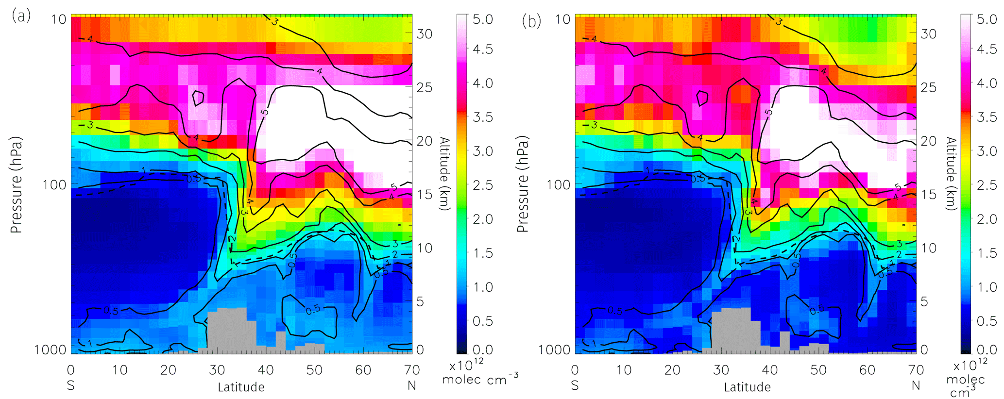
Figure 14Two meridional cross sections over the Tibetan Plateau, located at 84.25∘ E on 25 February 2008, 06:00 UTC. The colours indicate the ozone concentration from the free model run (a) and the assimilation of both GOME-2 and OMI (b). The solid contours show the ozone concentrations from the ERA-Interim reanalysis. The dashed line shows the thermal tropopause.
To demonstrate the performance of the assimilation algorithm we analysed the results for a day above the Tibetan Plateau (located between 30 and 40∘ N), where a highly dynamical atmosphere exists. This makes it an interesting area to study atmospheric dynamics, and difficult for modelling so it can serve as a test case to see if the dynamics in the model are correctly implemented. On 25 February 2008 a stratosphere–troposphere exchange event was observed in GOME-2 data (Chen et al., 2013), which can also be observed in the assimilation output. In Fig. 14, ozone concentrations from the ERA-Interim reanalysis (Dee et al., 2011; Dragani, 2011) are plotted as contours over the ozone concentrations from the model runs with and without simultaneous assimilation of GOME-2 and OMI. There is a significantly better agreement between the two datasets north of 35∘ N at pressure levels between 70 and 10 hPa. Even though the GOME-2 and OMI instruments have limited sensitivity in the troposphere, the tropospheric ozone concentrations of the ERA-Interim reanalysis and assimilated tropospheric ozone are in better agreement north of the Tibetan Plateau. There are also two stratosphere–troposphere exchanges (STE) visible, at 30 and 60∘ N. These STEs are associated with strong jet-streams (perpendicular to the page) reaching wind speeds of up to 50 m s−1 at 250 hPa.
When two instruments are assimilated simultaneously, their differences should be taken into account. For example, the algorithms used for the retrieval of GOME-2 and OMI ozone profiles both produce partial columns. However, the number of layers in the retrievals differ and the sensitivity of the retrieval is expressed by the averaging kernel. Both the different vertical resolution and the averaging kernel are incorporated into the observation operator H. Both instruments have different horizontal resolution, something which has not been taken into account in the current version of the assimilation algorithm. The measurement principle of GOME-2 (i.e. a cross-track scanning mirror) is different than that of OMI (i.e. a fixed 2-D CCD detector). As a result, the ground pixel size of GOME-2 is constant, while that of OMI varies across the track. Therefore, the representation error of OMI will increase towards the edges of the swath. The effect of the changing OMI footprint size has not been investigated. To get an idea of the sub-grid-cell variation in the ozone concentration, we performed a small experiment where we assimilated the same observations (i.e. GOME-2 and OMI) into TM5 running on a grid (as opposed to the standard used in this article). The total column standard deviation of the six grid cells covered by a single grid cell is much smaller than the error on the total column. Therefore, the representation error due to the large grid cells is not significant. A more thorough check on the instruments behaviour throughout time might have revealed the effect of the OMI L0 to L1b processor update sooner. The threshold of the parameter in the OmF filter might be made instrument and time dependent in order to minimize the effect on the number of assimilated pixels.
Two different instruments can be biased with respect to each other. In order to minimize the bias, a bias correction scheme has been implemented with respect to ozone sondes. We used cloud-free observations (max. cloud fraction 0.20) for the bias correction in order to get a maximum amount of information from the troposphere. As a consequence, we could not use all available sondes in deriving the bias correction. Sudden changes in the bias correction parameters are visible at the start of the year, when the parameters are changed. To minimize these changes, it might be worthwhile to implement an interpolation scheme for the bias correction parameters similar as for the MSR data (see van der A et al., 2010, 2015).
The model can run a full chemistry scheme, but instead a parameterized chemistry scheme has been used in favour of speed. Another possibility to increase the accuracy of the model is to increase the horizontal resolution from the current (long. × lat.) to for example. However, in both cases it might be necessary to reduce the vertical resolution of the model to keep the computational cost at an acceptable level.
The model covariance matrix is also an expensive step in the assimilation algorithm. We have reduced the calculation cost by parameterizing it into a time-dependent error field and a time-independent correlation field. The data from April 2008 was used to derive the correlations, which were then used for the whole assimilation period. The assumption that the derived correlations are constant throughout time has not been tested.
An algorithm for the simultaneous assimilation of GOME-2 and OMI ozone profiles has been described. The algorithm uses a Kalman filter to assimilate the ozone profiles into the TM5 chemical transport model. Compared to previous versions, the algorithm is significantly updated. The observational error has been characterized using a newly developed in-flight calibration method. Since the Kalman filter equations are too expensive to calculate directly for the current setup, the model covariance matrix is divided into a time-dependent error field and a time independent correlation field. The time evolution is applied to the error field only, while the correlation is assumed to be constant. The model error growth is modelled by a new function that prevents the error from increasing indefinitely, and the correlation field has been newly derived using the NMC method. Large biases between retrievals of the two instruments might destabilize the assimilation. To avoid this, a bias correction using global ozone sonde observations has been applied to the retrieved ozone profiles before assimilation.
Four model runs were performed spanning the years between 2008 and 2011: without assimilation, with assimilation of GOME-2 only, with assimilation of OMI profiles only and with simultaneous assimilation of both GOME-2 and OMI profiles. Depending on the altitude, the OmF and OmA for one instrument might be larger than the other, which might change in the course of time. Assimilating the observations from these instruments simultaneously increases the overall sensitivity of the assimilation. Two notable instrumental effects are the band 1A/1B wavelength shift for GOME-2, which causes a significant decrease in OmF and OmA. For OMI, after the L0 to L1b processor update on 1 February 2010, the uncertainty in the observations is too small with respect to the method of in-flight validation of the uncertainties presented in this paper. This caused a decrease in the number of assimilated observations for both GOME-2 and OMI. The expected and observed OmF and OmA are more similar for the combined assimilation than for the separate assimilations. Validation with sondes from the WOUDC shows that the combined assimilation performs better than the single sensor assimilation in the region between 100 and 10 hPa where GOME-2 and OMI are most sensitive. The ozone concentrations in the troposphere are also affected by the assimilation, even though the instruments have limited sensitivity in that region. The biases of the assimilated ozone fields are smaller than those of the observations. The assimilated ozone fields are produced at regular time intervals and have no missing data. Despite the limited vertical resolution of GOME-2 and OMI, a case study of an STE over the Tibetan Plateau shows that the assimilation of ozone profiles can improve the ozone distribution in a highly dynamical region.
OMI L2 ozone profiles are operationally retrieved and can be obtained from NASA's Goddard Earth Sciences (GES) Data and Information Services Center (DISC) on-line archive at https://aura.gesdisc.eosdis.nasa.gov/data/Aura_OMI_Level2/OMO3PR.003/. GOME-2 L2 ozone profiles are specifically retrieved for this research and can be obtained by contacting the author. Although not used in this research, operationally retrieved GOME-2 ozone profiles can be retrieved from EUMETSATs ACSAF (https://acsaf.org/index.html), but note that a registration is required.
The authors declare that they have no conflict of interest.
The authors acknowledge all scientists and institutes who contributed their
ozone sonde data to the World Ozone and Ultraviolet Radiation Data Centre
(WOUDC, WMO/GAW, 2016), and the Meteorological Service of Canada for hosting this
important public database. The authors would also like to thank Pepijn
Veefkind for his comments in preparation of this paper. EUMETSAT is
acknowledged for providing the GOME-2 L1 data and Olaf Tuinder and Robert van
Versendaal for their help in the retrieval of the GOME-2 ozone profiles. The
Dutch–Finnish OMI instrument is part of the NASA EOS Aura satellite payload.
The OMI ozone profiles (OMO3PR, v003) were retrieved at NASA Goddard Earth
Sciences Data and Information Services Center (GES DISC) and accessed from
the local storage at the Royal Netherlands Meteorological Institute (KNMI).
Part of this research has been funded by the Ozone_cci project
(http://www.esa-ozone-cci.org), which is part of the Climate Change
Initiative (CCI) programme of the European Space Agency
(ESA).
Edited by: Michel Van
Roozendael
Reviewed by: two anonymous referees
Bhartia, P. K., McPeters, R. D., Flynn, L. E., Taylor, S., Kramarova, N. A., Frith, S., Fisher, B., and DeLand, M.: Solar Backscatter UV (SBUV) total ozone and profile algorithm, Atmos. Meas. Tech., 6, 2533–2548, https://doi.org/10.5194/amt-6-2533-2013, 2013. a
Bovensmann, H., Burrows, J. P., Buchwitz, M., Frerick, J., Noël, S., Rozanov, V. V., Chance, K. V., and Goede, A. P. H.: SCIAMACHY: mission objectives and measurement modes, J. Atmos. Sci., 56, 127–150, https://doi.org/10.1175/1520-0469(1999)056<0127:SMOAMM>2.0.CO;2, 1999. a
Burrows, J. P., Weber, M., Buchwitz, M., Rozanov, V., Ladstätter-Weißenmayer, A., Richter, A., Debeek, R., Hoogen, R., Bramstedt, K., Eichmann, K.-U., Eisinger, M., and Perner, D.: The Global Ozone Monitoring Experiment (GOME): mission concept and first scientific results, J. Atmos. Sci., 56, 151–175, https://doi.org/10.1175/1520-0469(1999)056<0151:TGOMEG>2.0.CO;2, 1999. a
Callies, J., Corpaccioli, E., Eisinger, M., Hahne, A., and Lefebvre, A.: GOME-2 – Metop's second-generation sensor for operational ozone monitoring, ESA Bull.-Eur. Space, 102, 28–36, 2000. a, b
Cariolle, D. and Teyssèdre, H.: A revised linear ozone photochemistry parameterization for use in transport and general circulation models: multi-annual simulations, Atmos. Chem. Phys., 7, 2183–2196, https://doi.org/10.5194/acp-7-2183-2007, 2007. a
Chen, X., Añel, J. A., Su, Z., de la Torre, L., Kelder, H., van Peet, J., and Ma, Y.: The deep atmospheric boundary layer and its significance to the stratosphere and troposphere exchange over the Tibetan Plateau, PLoS One, 8, e56909, https://doi.org/10.1371/journal.pone.0056909, 2013. a
de Laat, A. T. J., van der A, R. J., and van Weele, M.: Evaluation of tropospheric ozone columns derived from assimilated GOME ozone profile observations, Atmos. Chem. Phys., 9, 8105–8120, https://doi.org/10.5194/acp-9-8105-2009, 2009. a, b, c, d
Dee, D. P., Uppala, S. M., Simmons, A. J., Berrisford, P., Poli, P., Kobayashi, S., Andrae, U., Balmaseda, M. A., Balsamo, G., Bauer, P., Bechtold, P., Beljaars, A. C. M., van de Berg, L., Bidlot, J., Bormann, N., Delsol, C., Dragani, R., Fuentes, M., Geer, A. J., Haimberger, L., Healy, S. B., Hersbach, H., Hólm, E. V., Isaksen, L., Kållberg, P., Köhler, M., Matricardi, M., McNally, A. P., Monge-Sanz, B. M., Morcrette, J.-J., Park, B.-K., Peubey, C., de Rosnay, P., Tavolato, C., Thépaut, J.-N., and Vitart, F.: The ERA-Interim reanalysis: configuration and performance of the data assimilation system, Q. J. Roy. Meteor. Soc., 137, 553–597, https://doi.org/10.1002/qj.828, 2011. a, b
Dethof, A. and Hólm, E. V.: Ozone assimilation in the ERA-40 reanalysis project, Q. J. Roy. Meteor. Soc., 130, 2851–2872, https://doi.org/10.1256/qj.03.196, 2004. a
Dragani, R.: On the quality of the ERA-Interim ozone reanalyses: comparisons with satellite data, Q. J. Roy. Meteor. Soc., 137, 1312–1326, https://doi.org/10.1002/qj.821, 2011. a, b, c
Errera, Q., Daerden, F., Chabrillat, S., Lambert, J. C., Lahoz, W. A., Viscardy, S., Bonjean, S., and Fonteyn, D.: 4D-Var assimilation of MIPAS chemical observations: ozone and nitrogen dioxide analyses, Atmos. Chem. Phys., 8, 6169–6187, https://doi.org/10.5194/acp-8-6169-2008, 2008. a
Eskes, H. J., Velthoven, P. F. J. V., Valks, P. J. M., and Kelder, H. M.: Assimilation of GOME total-ozone satellite observations in a three-dimensional tracer-transport model, Q. J. Roy. Meteor. Soc., 129, 1663–1681, https://doi.org/10.1256/qj.02.14, 2003. a, b, c, d
Evensen, G.: The Ensemble Kalman Filter: theoretical formulation and practical implementation, Ocean Dynam., 53, 343–367, https://doi.org/10.1007/s10236-003-0036-9, 2003. a
Flemming, J., Huijnen, V., Arteta, J., Bechtold, P., Beljaars, A., Blechschmidt, A.-M., Diamantakis, M., Engelen, R. J., Gaudel, A., Inness, A., Jones, L., Josse, B., Katragkou, E., Marecal, V., Peuch, V.-H., Richter, A., Schultz, M. G., Stein, O., and Tsikerdekis, A.: Tropospheric chemistry in the Integrated Forecasting System of ECMWF, Geosci. Model Dev., 8, 975–1003, https://doi.org/10.5194/gmd-8-975-2015, 2015. a
Fortuin, J. P. F. and Kelder, H.: An ozone climatology based on ozonesonde and satellite measurements, J. Geophys. Res., 103, 31709–31734, https://doi.org/10.1029/1998JD200008, 1998. a
Hoogen, R., Rozanov, V. V., and Burrows, J. P.: Ozone profiles from GOME satellite data: algorithm description and first validation, J. Geophys. Res., 104, 8263–8280, https://doi.org/10.1029/1998JD100093, 1999. a
Houtekamer, P. L. and Zhang, F.: Review of the Ensemble Kalman Filter for Atmospheric Data Assimilation, Mon. Weather Rev., 144, 4489–4532, https://doi.org/10.1175/MWR-D-15-0440.1, 2016. a
Huijnen, V., Williams, J., van Weele, M., van Noije, T., Krol, M., Dentener, F., Segers, A., Houweling, S., Peters, W., de Laat, J., Boersma, F., Bergamaschi, P., van Velthoven, P., Le Sager, P., Eskes, H., Alkemade, F., Scheele, R., Nédélec, P., and Pätz, H.-W.: The global chemistry transport model TM5: description and evaluation of the tropospheric chemistry version 3.0, Geosci. Model Dev., 3, 445–473, https://doi.org/10.5194/gmd-3-445-2010, 2010. a
Huijnen, V., Flemming, J., Chabrillat, S., Errera, Q., Christophe, Y., Blechschmidt, A.-M., Richter, A., and Eskes, H.: C-IFS-CB05-BASCOE: stratospheric chemistry in the Integrated Forecasting System of ECMWF, Geosci. Model Dev., 9, 3071–3091, https://doi.org/10.5194/gmd-9-3071-2016, 2016. a
Krol, M., Houweling, S., Bregman, B., van den Broek, M., Segers, A., van Velthoven, P., Peters, W., Dentener, F., and Bergamaschi, P.: The two-way nested global chemistry-transport zoom model TM5: algorithm and applications, Atmos. Chem. Phys., 5, 417–432, https://doi.org/10.5194/acp-5-417-2005, 2005. a, b
Kroon, M., de Haan, J. F., Veefkind, J. P., Froidevaux, L., Wang, R., Kivi, R., and Hakkarainen, J. J.: Validation of operational ozone profiles from the ozone monitoring instrument, J. Geophys. Res.-Atmos., 116, D18305, https://doi.org/10.1029/2010JD015100, 2011. a
Lefever, K., van der A, R., Baier, F., Christophe, Y., Errera, Q., Eskes, H., Flemming, J., Inness, A., Jones, L., Lambert, J.-C., Langerock, B., Schultz, M. G., Stein, O., Wagner, A., and Chabrillat, S.: Copernicus stratospheric ozone service, 2009–2012: validation, system intercomparison and roles of input data sets, Atmos. Chem. Phys., 15, 2269–2293, https://doi.org/10.5194/acp-15-2269-2015, 2015. a
Lerot, C., Van Roozendael, M., Spurr, R., Loyola, D., Coldewey-Egbers, M., Kochenova, S., van Gent, J., Koukouli, M., Balis, D., Lambert, J.-C., Granville, J., and Zehner, C.: Homogenized total ozone data records from the European sensors GOME/ERS-2, SCIAMACHY/Envisat, and GOME-2/MetOp-A, J. Geophys. Res.-Atmos., 119, 1639–1662, https://doi.org/10.1002/2013JD020831, 2014. a
Levelt, P. F., van den Oord, G. H. J., Dobber, M. R., Malkki, A., Visser, H., de Vries, J., Stammes, P., Lundell, J. O. V., and Saari, H.: The ozone monitoring instrument, IEEE T. Geosci. Remote, 44, 1093–1101, https://doi.org/10.1109/TGRS.2006.872333, 2006. a, b
Migliorini, S.: On the equivalence between radiance and retrieval assimilation, Mon. Weather Rev., 140, 258–265, https://doi.org/10.1175/MWR-D-10-05047.1, 2012. a, b
Miles, G. M., Siddans, R., Kerridge, B. J., Latter, B. G., and Richards, N. A. D.: Tropospheric ozone and ozone profiles retrieved from GOME-2 and their validation, Atmos. Meas. Tech., 8, 385–398, https://doi.org/10.5194/amt-8-385-2015, 2015. a
Miyazaki, K., Eskes, H. J., Sudo, K., Takigawa, M., van Weele, M., and Boersma, K. F.: Simultaneous assimilation of satellite NO2, O3, CO, and HNO3 data for the analysis of tropospheric chemical composition and emissions, Atmos. Chem. Phys., 12, 9545–9579, https://doi.org/10.5194/acp-12-9545-2012, 2012. a
Munro, R., Lang, R., Klaes, D., Poli, G., Retscher, C., Lindstrot, R., Huckle, R., Lacan, A., Grzegorski, M., Holdak, A., Kokhanovsky, A., Livschitz, J., and Eisinger, M.: The GOME-2 instrument on the Metop series of satellites: instrument design, calibration, and level 1 data processing – an overview, Atmos. Meas. Tech., 9, 1279–1301, https://doi.org/10.5194/amt-9-1279-2016, 2016. a, b
Parrish, D. F. and Derber, J. C.: The National Meteorological Center's Spectral Statistical-Interpolation Analysis System, Mon. Weather Rev., 120, 1747–1763, https://doi.org/10.1175/1520-0493(1992)120<1747:TNMCSS>2.0.CO;2, 1992. a
Rodgers, C. D.: Characterization and error analysis of profiles retrieved from remote sounding measurements, J. Geophys. Res.-Atmos., 95, 5587–5595, https://doi.org/10.1029/JD095iD05p05587, 1990. a
Rodgers, C. D.: Inverse Methods for Atmospheric Sounding, World Scientific Publishing, Singapore, 2000. a
Segers, A. J., Eskes, H. J., van der A, R. J., van Oss, R. F., and van Velthoven, P. F. J.: Assimilation of GOME ozone profiles and a global chemistry-transport model using a Kalman filter with anisotropic covariance, Q. J. Roy. Meteor. Soc., 131, 477–502, https://doi.org/10.1256/qj.04.92, 2005. a, b, c, d, e, f, g, h, i, j
Sofieva, V. F., Rahpoe, N., Tamminen, J., Kyrölä, E., Kalakoski, N., Weber, M., Rozanov, A., von Savigny, C., Laeng, A., von Clarmann, T., Stiller, G., Lossow, S., Degenstein, D., Bourassa, A., Adams, C., Roth, C., Lloyd, N., Bernath, P., Hargreaves, R. J., Urban, J., Murtagh, D., Hauchecorne, A., Dalaudier, F., van Roozendael, M., Kalb, N., and Zehner, C.: Harmonized dataset of ozone profiles from satellite limb and occultation measurements, Earth Syst. Sci. Data, 5, 349–363, https://doi.org/10.5194/essd-5-349-2013, 2013. a
Uppala, S. M., Kållberg, P. W., Simmons, A. J., Andrae, U., Bechtold, V. D., Fiorino, M., Gibson, J. K., Haseler, J., Hernandez, A., Kelly, G. A., Li, X., Onogi, K., Saarinen, S., Sokka, N., Allan, R. P., Andersson, E., Arpe, K., Balmaseda, M. A., Beljaars, A. C. M., Van De Berg, L., Bidlot, J., Bormann, N., Caires, S., Chevallier, F., Dethof, A., Dragosavac, M., Fisher, M., Fuentes, M., Hagemann, S., Hólm, E., Hoskins, B. J., Isaksen, L., Janssen, P. A. E. M., Jenne, R., Mcnally, A. P., Mahfouf, J.-F., Morcrette, J.-J., Rayner, N. A., Saunders, R. W., Simon, P., Sterl, A., Trenberth, K. E., Untch, A., Vasiljevic, D., Viterbo, P., and Woollen, J.: The ERA-40 re-analysis, Q. J. Roy. Meteor. Soc., 131, 2961–3012, https://doi.org/10.1256/qj.04.176, 2005. a
van der A, R. J., Allaart, M. A. F., and Eskes, H. J.: Multi sensor reanalysis of total ozone, Atmos. Chem. Phys., 10, 11277–11294, https://doi.org/10.5194/acp-10-11277-2010, 2010. a, b
van der A, R. J., Allaart, M. A. F., and Eskes, H. J.: Extended and refined multi sensor reanalysis of total ozone for the period 1970–2012, Atmos. Meas. Tech., 8, 3021–3035, https://doi.org/10.5194/amt-8-3021-2015, 2015. a, b, c
van Peet, J. C. A., van der A, R. J., Tuinder, O. N. E., Wolfram, E., Salvador, J., Levelt, P. F., and Kelder, H. M.: Ozone ProfilE Retrieval Algorithm (OPERA) for nadir-looking satellite instruments in the UV–VIS, Atmos. Meas. Tech., 7, 859–876, https://doi.org/10.5194/amt-7-859-2014, 2014. a, b
WMO: Implementation plan for the global observing system for climate in support of the UNFCCC (2010 update), Report nr. GCOS-138, Geneva, Switzerland, 2010. a
WOUDC, WMO/GAW: WMO/GAW Ozone Monitoring Community, World Meteorological Organization-Global Atmosphere Watch Program (WMO-GAW)/World Ozone and Ultraviolet Radiation Data Centre (WOUDC) (Data), a list of all contributors is available on the website, available at: http://woudc.org, https://doi.org/10.14287/10000001, last access: 15 April 2016. a, b, c