Effective radiative forcing in the aerosol–climate model CAM5.3-MARC-ARG

We quantify the effective radiative forcing (ERF) of anthropogenic aerosols modelled by the aerosol–climate model CAM5.3-MARC-ARG. CAM5.3-MARC-ARG is a new configuration of the Community Atmosphere Model version 5.3 (CAM5.3) in which the default aerosol module has been replaced by the two-Moment, Multi-Modal, Mixing-state-resolving Aerosol model for Research of Climate (MARC). CAM5.3-MARC-ARG uses the ARG aerosol-activation scheme, consistent with the default configuration of CAM5.3. We compute differences between simulations using year-1850 aerosol emissions and simulations using year-2000 aerosol emissions in order to assess the radiative effects of anthropogenic aerosols. We compare the aerosol lifetimes, aerosol column burdens, cloud properties, and radiative effects produced by CAM5.3-MARC-ARG with those produced by the default configuration of CAM5.3, which uses the modal aerosol module with three log-normal modes (MAM3), and a configuration using the modal aerosol module with seven log-normal modes (MAM7). Compared with MAM3 and MAM7, we find that MARC produces stronger cooling via the direct radiative effect, the shortwave cloud radiative effect, and the surface albedo radiative effect; similarly, MARC produces stronger warming via the longwave cloud radiative effect. Overall, MARC produces a global mean net ERF of $-\mathrm{1.79}\pm \mathrm{0.03}$ W m⁻², which is stronger than the global mean net ERF of $-\mathrm{1.57}\pm \mathrm{0.04}$ W m⁻² produced by MAM3 and $-\mathrm{1.53}\pm \mathrm{0.04}$ W m⁻² produced by MAM7. The regional distribution of ERF also differs between MARC and MAM3, largely due to differences in the regional distribution of the shortwave cloud radiative effect. We conclude that the specific representation of aerosols in global climate models, including aerosol mixing state, has important implications for climate modelling.

1 Introduction

Aerosol particles influence the earth's climate system by perturbing its radiation budget. There are three primary mechanisms by which aerosols interact with radiation. First, aerosols interact directly with radiation by scattering and absorbing solar and thermal infrared radiation (Haywood and Boucher, 2000). Second, aerosols interact indirectly with radiation by perturbing clouds, acting as the cloud condensation nuclei on which cloud droplets form and the ice nuclei that facilitate freezing of cloud droplets (Fan et al., 2016; Rosenfeld et al., 2014); for example, an aerosol-induced increase in cloud cover would lead to increased scattering of “shortwave” solar radiation and increased absorption of “longwave” thermal infrared radiation. Third, aerosols can influence the albedo of the earth's surface; for example, the deposition of absorbing aerosol on snow reduces the albedo of the snow, causing more solar radiation to be absorbed at the earth's surface (Jiao et al., 2014).

The “effective radiative forcing” (ERF) of anthropogenic aerosols, defined as the top-of-atmosphere radiative effect caused by anthropogenic emissions of aerosols and aerosol precursors, is often used to quantify the radiative effects of aerosols (Boucher et al., 2013). In contrast to instantaneous radiative forcing, ERF allows rapid adjustments – including changes to clouds – to occur (Sherwood et al., 2015). The anthropogenic aerosol ERF is approximately equivalent to “the radiative flux perturbation associated with a change from preindustrial to present-day [aerosol emissions], calculated in a global climate model using fixed sea surface temperature” (Haywood et al., 2009). This approach “allows clouds to respond to the aerosol while [sea] surface temperature is prescribed” (Ghan, 2013).

The primary tools available for investigating the anthropogenic aerosol ERF are state-of-the-art global climate models. However, there is widespread disagreement among these models, especially regarding the magnitude of anthropogenic aerosol ERF (Quaas et al., 2009; Shindell et al., 2013). The magnitude of the ERF of anthropogenic aerosols is highly uncertain; estimates of the global mean anthropogenic aerosol ERF range from −1.9 to −0.1 W m⁻² (Boucher et al., 2013). Much of this uncertainty can be attributed to uncertainty in pre-industrial aerosol emissions (Carslaw et al., 2013). Model parameterisations constitute another large source of uncertainty. Of particular importance are model parameterisations relating to aerosol–cloud interactions, such as the aerosol-activation scheme (Rothenberg et al., 2018), the choice of autoconversion threshold radius (Golaz et al., 2011), and constraints on the minimum cloud droplet number concentration (Hoose et al., 2009). The detailed representation of aerosols also likely plays an important role, because the aerosol particle size and chemical composition determine hygroscopicity and hence influence aerosol activation (Petters and Kreidenweis, 2007).

The present-day anthropogenic aerosol ERF partially masks the warming effects of anthropogenic greenhouse gases. Therefore, the large uncertainty in the anthropogenic aerosol ERF is a major source of uncertainty in estimates of equilibrium climate sensitivity and projections of future climate (Andreae et al., 2005). Furthermore, the anthropogenic aerosol ERF is regionally inhomogeneous, adding another source of uncertainty in climate projections (Shindell, 2014). The regional inhomogeneity of the anthropogenic aerosol ERF has also likely influenced rainfall patterns during the 20th century (Wang, 2015). In order to improve the understanding of current and future climate, including rainfall patterns, it is necessary to improve the understanding of the magnitude and regional distribution of the anthropogenic aerosol ERF.

In this paper, we investigate the uncertainty in anthropogenic aerosol ERF associated with the representation of aerosols in global climate models. In particular, we assess the aerosol radiative effects produced by a new configuration of the Community Atmosphere Model version 5.3 (CAM5.3). In this new configuration – CAM5.3-MARC-ARG – the default modal aerosol module has been replaced with the two-Moment, Multi-Modal, Mixing-state-resolving Aerosol model for Research of Climate (MARC). We compare the aerosol fields and aerosol radiative effects produced by CAM5.3-MARC-ARG with those produced by the default modal aerosol module in CAM5.3.

2 Methodology

2.1 Modal aerosol modules (MAM3 and MAM7)

The Community Earth System Model version 1.2.2 (CESM 1.2.2) contains the Community Atmosphere Model version 5.3 (CAM5.3). Within CAM5.3, the default aerosol module is a modal aerosol module that parameterises the aerosol size distribution using three log-normal modes (MAM3), each assuming a total internal mixture of a set of fixed chemical species (Liu et al., 2012). Optionally, a more detailed modal aerosol module with seven log-normal modes (MAM7; Liu et al., 2012) can be used instead of MAM3. More recently, a version containing four modes (MAM4; Liu et al., 2016) has also been coupled to CAM5.3, but we do not consider MAM4 in this study.

The seven modes included in MAM7 are Aitken, accumulation, primary carbon, fine soil dust, fine sea salt, coarse soil dust, and coarse sea salt. Depending on the mode, MAM7 simulates the mass mixing ratios of internally mixed sulfate, ammonium, primary organic matter, secondary organic matter, black carbon, soil dust, and sea salt (Liu et al., 2012).

In MAM3, four simplifications are made. First, the primary carbon mode is merged into the accumulation mode. Second, the fine soil dust and fine sea salt modes are also merged into the accumulation mode. Third, the coarse soil dust and coarse sea salt modes are merged to form a single coarse mode. Fourth, ammonium is implicitly included via sulfate and is no longer explicitly simulated. As a result, MAM3 simulates just three modes: Aitken, accumulation, and coarse. This reduces the computational expense of the model.

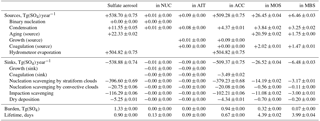
Table 1 Global mass budgets and lifetimes of sulfate aerosol for the year-2000 MARC simulation, showing values for total sulfate aerosol and sulfate aerosol in each mode. Negative values indicate sinks. Standard errors are calculated using the annual global total for each simulation year; for each lifetime (calculated as Burden divided by Sinks), the combined standard error is calculated following Hogan (2006). The processes acting as sources and sinks are summarised in Fig. 1a. Growth and coagulation transfer sulfate between modes but do not directly influence the total sulfate aerosol mass. Due to hydrometeor evaporation, scavenging does not necessarily result in permanent removal from the atmosphere in the form of wet deposition. (It is not possible to calculate the net wet deposition rate, because the aqueous oxidation of sulfur dioxide and scavenging of gas-phase sulfuric acid also contribute to the sulfate dissolved in the hydrometeors, as shown in Fig. 1a.) Corresponding results for the year-1850 MARC simulation are shown in Table S1.

In this paper, we often refer to MAM3 and MAM7 collectively as “MAM”. The MAM-simulated aerosols interact with radiation, allowing aerosol direct and semi-direct effects to be represented. The aerosols can act as cloud condensation nuclei via the ARG aerosol-activation scheme (Abdul-Razzak and Ghan, 2000); sulfate and dust also act as ice nuclei. Via such activation, the aerosols are coupled to the stratiform cloud microphysics (Gettelman et al., 2010; Morrison and Gettelman, 2008), allowing aerosol indirect effects on stratiform clouds to be represented. These indirect effects dominate the anthropogenic aerosol ERF in CAM version 5.1 (CAM5.1; Ghan et al., 2012). In comparison with many other global climate models, the anthropogenic aerosol ERF in CAM5.1 is relatively strong (Shindell et al., 2013).

2.2 The two-Moment, Multi-Modal, Mixing-state-resolving Aerosol model for Research of Climate (MARC)

The two-Moment, Multi-Modal, Mixing-state-resolving Aerosol model for Research of Climate (MARC), which is based on the aerosol microphysical scheme developed by Ekman et al. (2004, 2006) and Kim et al. (2008), simulates the evolution of mixtures of aerosol species. Previous versions of MARC have been used both in cloud-resolving model simulations (Ekman et al., 2004, 2006, 2007; Engström et al., 2008; Wang, 2005a, b) and in global climate model simulations (Kim et al., 2008, 2014; Ekman et al., 2012). Recently, an updated version of MARC has been coupled to CAM5.3 within CESM1.2.2 (Rothenberg et al., 2018).

In contrast to MAM, MARC tracks the number concentrations and mass concentrations of both externally mixed and internally mixed aerosol modes with assumed log-normal size distributions. The externally mixed modes include three pure sulfate modes (nucleation, Aitken, and accumulation), pure organic carbon (OC), and pure black carbon (BC). The internally mixed modes include mixed organic carbon plus sulfate (MOS) and mixed black carbon plus sulfate (MBS). In the MOS mode, it is assumed that the organic carbon and sulfate are mixed homogeneously within each particle; in the MBS mode, it is assumed that each particle contains a black carbon core surrounded by a sulfate shell. Sea salt and mineral dust are represented using sectional single-moment schemes, each with four size bins (Albani et al., 2014; Mahowald et al., 2006; Scanza et al., 2015). Table 1 of Rothenberg et al. (2018) contains details of the size distribution, density, and hygroscopicity of each mode. It is assumed that the pure OC and pure BC modes are hydrophobic (Petters and Kreidenweis, 2007; Rothenberg et al., 2018).

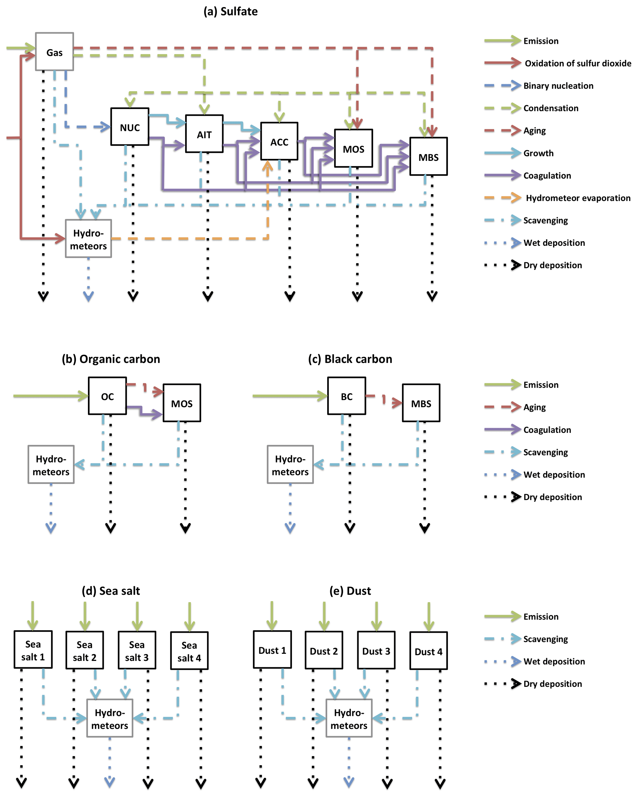
Figure 1 Physical and chemical processes represented by MARC, organised by chemical species: (a) sulfate, (b) organic carbon, (c) black carbon, (d) sea salt, and (e) mineral dust. Black boxes represent aerosol modes: nucleation-mode sulfate (NUC), Aitken-mode sulfate (AIT), accumulation-mode sulfate (ACC), internally mixed organic carbon plus sulfate (MOS), internally mixed black carbon plus sulfate (MBS), pure organic carbon (OC), pure black carbon (BC), four sea salt modes, and four mineral dust modes. Grey boxes represent non-aerosol states; sulfate can exist in the gas phase (as sulfuric acid), and all five chemical species can be scavenged by hydrometeors. The arrows illustrating physical and chemical processes are listed in the legend to the right of each row. Emission of sulfate (as gas-phase sulfuric acid) and oxidation of sulfur dioxide (including both gas-phase and aqueous processes) are handled by the sulfur chemistry scheme in CAM5.3. Emissions of OC include a contribution from volatile organic compounds. For sulfate, organic carbon, and black carbon, “scavenging” includes nucleation scavenging by stratiform clouds (handled by the aerosol-activation scheme) and nucleation scavenging by convective clouds (assuming a constant supersaturation of 0.1 %) in addition to impaction scavenging; for sea salt and dust, “scavenging” refers to impaction scavenging only. “Dry deposition” includes gravitational settling. Further details are provided in Sect. 2.2 of this paper and Sect. 2.1 of Rothenberg et al. (2018).

Sea salt emissions follow the default scheme used by MAM (Liu et al., 2012), based on simulated wind speed and sea surface temperature. Dust emissions follow the tuning of Albani et al. (2014), based on simulated wind speed and soil properties, including soil moisture and vegetation cover. Emissions of sulfur dioxide, dimethyl sulfide, sulfate (as gas-phase sulfuric acid), organic carbon aerosol, black carbon aerosol, and volatile organic compounds (such as isoprene and monoterpene) are prescribed. The volatile organic compounds are converted upon emission into pure OC.

The aerosol removal processes represented by MARC – including nucleation scavenging by both stratiform and convective clouds, impaction scavenging by precipitation, and dry deposition – are based on aerosol size and mixing state. Evaporation of cloud and rain drops results in resuspension of sulfate aerosol in the accumulation mode.

Figure 1 summarises the physical and chemical processes represented by MARC. Further details about the formulation of MARC, as well as validation of its simulated aerosol fields compared with observations, can be found in the body and Supplement of Rothenberg et al. (2018).

Whereas previous versions of MARC represented only direct interactions between aerosols and radiation (Kim et al., 2008), an important feature of the new version of MARC is that the aerosols also interact indirectly with radiation via clouds. The MARC-simulated aerosols interact with stratiform cloud microphysics via the default stratiform cloud microphysics scheme (Gettelman et al., 2010; Morrison and Gettelman, 2008), as would be the case for the default MAM3 configuration of CAM5.3. Various aerosol-activation schemes can be used with MARC (Rothenberg et al., 2018), including versions of a recently developed scheme based on polynomial chaos expansion (Rothenberg and Wang, 2016, 2017). The choice of activation scheme can substantially influence the ERF (Rothenberg et al., 2018). In order to facilitate the comparison between the MAM and MARC aerosol modules, we have chosen to keep the activation scheme constant in this study; as is the case for the MAM simulations, the ARG activation scheme (Abdul-Razzak and Ghan, 2000) is also used for the MARC simulations. We refer to this configuration as “CAM5.3-MARC-ARG”.

2.3 Simulations

In order to compare results from MAM3, MAM7, and MARC, six CAM5.3 simulations are performed:

• 1.

  “MAM3_2000”, which uses MAM3 with year-2000 aerosol (including aerosol precursor) emissions;

• 2.

  “MAM7_2000”, which uses MAM7 with year-2000 aerosol emissions;

• 3.

  “MARC_2000”, which uses MARC with year-2000 aerosol emissions;

• 4.

  “MAM3_1850”, which uses MAM3 with year-1850 aerosol emissions;

• 5.

  “MAM7_1850”, which uses MAM7 with year-1850 aerosol emissions; and

• 6.

  “MARC_1850”, which uses MARC with year-1850 aerosol emissions.

The three simulations using year-2000 emissions, referred to as the “year-2000 simulations”, facilitate the comparison of aerosol fields and cloud fields; the three simulations using year-1850 emissions, referred to as the “year-1850 simulations”, further facilitate the analysis of the aerosol radiative effects produced by MAM and MARC. In the figures and discussion of results, “2000–1850” and “Δ” both refer to differences between the year-2000 simulation and the year-1850 simulation for a given aerosol module (e.g. MARC_2000–MARC_1850). The “2000–1850” differences should be interpreted as aerosol-induced differences, arising due to changes in aerosol emissions alone; the only difference between the year-2000 simulations and the year-1850 simulations is the aerosol (including aerosol precursor) emissions.

In this study, we deliberately use identical emissions for MAM and MARC so that the influence of emission inventories can be minimised when the results are compared. The prescribed emissions for both MAM and MARC follow the default MAM emissions files, described in the Supplement of Liu et al. (2012) and based on Lamarque et al. (2010). (The ammonia emissions for the year-1850 MAM7 simulation are an exception, being based on the year-1850 ammonia emissions for the Coupled Model Intercomparison Project Phase 6.) This differs from Rothenberg et al. (2018), who used different emissions of organic carbon aerosol, black carbon aerosol, and volatile organic compounds.

For the MAM simulations, the emissions from forest fires and grass fires follow a vertical profile, as do sulfur emissions from the energy and industry sectors (Liu et al., 2012). For the MARC simulations, sulfur emissions follow the same vertical profile as for MAM, but all organic carbon, black carbon, and volatile organic compounds are emitted at the surface. 2.5 % of the sulfur dioxide is emitted as primary sulfate. The yield coefficients for the conversion of volatile organic compounds to organic carbon follow Liu et al. (2012). For the MAM simulations, the organic carbon aerosol emissions are converted to primary organic matter emissions using a scale factor of 1.4; for the MARC simulations, no such scale factor is applied. Mineral dust and sea salt emissions are not prescribed, being calculated “online”.

CESM 1.2.2, with CAM5.3, is used for all simulations. Greenhouse gas concentrations and sea surface temperatures (SSTs) are prescribed using year-2000 climatological values, based on the “F_2000_CAM5” component set. CAM5.3 is run at a horizontal resolution of $\mathrm{1.9}{}^{\circ }\times \mathrm{2.5}{}^{\circ }$, with 30 levels in the vertical direction. Clean-sky radiation diagnostics are included, facilitating the diagnosis of the direct radiative effect. The Cloud Feedback Model Intercomparison Project (CFMIP) Observational Simulator Package (COSP; Bodas-Salcedo et al., 2011) is switched on, although the COSP diagnostics are not analysed in this paper.

Each simulation is run for 32 years, and the first 2 years are excluded as spin-up. Hence, a period of 30 years is analysed. The ensemble of 30 annual means can be used to assess significance and calculate standard errors.

2.4 Diagnosis of radiative effects

Pairs of prescribed-SST simulations, with differing aerosol emissions, facilitate the diagnosis of anthropogenic aerosol ERF via the “radiative flux perturbation” approach (Haywood et al., 2009; Lohmann and Feichter, 2005). When “clean-sky” radiation diagnostics are available, the ERF can be decomposed into contributions from different radiative effects (Ghan, 2013). (We use the term “radiative forcing” only when referring to ERF, defined as the radiative flux perturbation between a simulation using year-1850 emissions and a simulation using year-2000 emissions; we use the term “radiative effect” more generally.)

Following Ghan (2013), the shortwave effective radiative forcing (ERF_SW) can be decomposed as follows:

$$\begin{array}{}\text{(1)}& {\displaystyle }{\text{ERF}}_{\mathrm{SW}}=\mathrm{\Delta }{\text{DRE}}_{\mathrm{SW}}+\mathrm{\Delta }{\text{CRE}}_{\mathrm{SW}}+\mathrm{\Delta }{\text{SRE}}_{\mathrm{SW}},\end{array}$$

where Δ refers to the 2000–1850 difference, DRE_SW is the direct radiative effect, CRE_SW is the clean-sky shortwave cloud radiative effect, and ΔSRE_SW is the 2000–1850 surface albedo radiative effect. These components are defined as follows:

$$\begin{array}{}\text{(2)}& {\displaystyle }& {\displaystyle }{\text{ERF}}_{\mathrm{SW}}=\mathrm{\Delta }F,\text{(3)}& {\displaystyle }& {\displaystyle }{\text{DRE}}_{\mathrm{SW}}=(F-F_{\mathrm{clean}}),\text{(4)}& {\displaystyle }& {\displaystyle }{\text{CRE}}_{\mathrm{SW}}=(F_{\mathrm{clean}}-F_{\mathrm{clean},\mathrm{clear}}),\text{(5)}& {\displaystyle }& {\displaystyle }\mathrm{\Delta }{\text{SRE}}_{\mathrm{SW}}=\mathrm{\Delta }{F}_{\mathrm{clean},\mathrm{clear}},\end{array}$$

where F is the net shortwave flux at top of atmosphere (TOA), F_clean is the clean-sky net shortwave flux at TOA, and F_{clean, clear} is the clean-sky clear-sky net shortwave flux at TOA. (“Clear-sky” refers to a hypothetical situation where clouds do not interact with radiation; “clean-sky” refers to a hypothetical situation where aerosols do not directly interact with radiation.)

The longwave effective radiative forcing (ERF_LW) is calculated as follows:

$$\begin{array}{}\text{(6)}& {\displaystyle }{\text{ERF}}_{\mathrm{LW}}=\mathrm{\Delta }L\approx \mathrm{\Delta }(L-L_{\mathrm{clear}})=\mathrm{\Delta }{\text{CRE}}_{\mathrm{LW}},\end{array}$$

where L is the net longwave flux at TOA, L_clear is the clear-sky net longwave flux at TOA, and CRE_LW is the longwave cloud radiative effect. Equation (6) assumes that aerosols and surface albedo changes do not influence the longwave flux at TOA, so that ΔL_clear≈0.

The net effective radiative forcing (ERF_SW+LW) is simply the sum of ERF_SW and ERF_LW:

$$\begin{array}{ll}{\displaystyle }{\text{ERF}}_{\mathrm{SW}+\mathrm{LW}}& {\displaystyle }=\mathrm{\Delta }\left(F+L\right)={\text{ERF}}_{\mathrm{SW}}+{\text{ERF}}_{\mathrm{LW}}\\ \text{(7)}& {\displaystyle }& {\displaystyle }\approx {\text{ERF}}_{\mathrm{SW}}+\mathrm{\Delta }{\text{CRE}}_{\mathrm{LW}}.\end{array}$$

All the quantities mentioned in Eqs. (1)–(7) are calculated at TOA.

We also consider absorption by aerosols in the atmosphere (AAA_SW), defined as follows:

$$\begin{array}{}\text{(8)}& {\displaystyle }{\text{AAA}}_{\mathrm{SW}}=\left(F-F_{\mathrm{clean}}\right)-\left(F^{\mathrm{surface}}-F_{\mathrm{clean}}^{\mathrm{surface}}\right),\end{array}$$

where F^surface is the net shortwave flux at the earth's surface, and $F_{\mathrm{clean}}^{\mathrm{surface}}$ is the clean-sky net shortwave flux at the earth's surface.

3 Results

To provide context for the discussion of the radiative effects, we first examine the aerosol mass budgets, lifetimes, and column burdens. We then focus on model output fields relating to different components of the ERF, taking each component in turn: the direct radiative effect, the cloud radiative effect, and the surface albedo radiative effect. When discussing each of these components, we also discuss related model fields; for example, in the section discussing the direct radiative effect, we also consider other fields related to direct aerosol–radiation interactions.

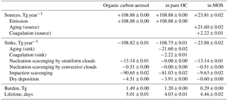
Table 2 Global mass budgets and lifetimes of organic carbon aerosol for the year-2000 MARC simulation, showing values for total organic carbon aerosol and organic carbon aerosol in each mode. The processes acting as sources and sinks are summarised in Fig. 1b. Emissions include volatile organic compounds converted to organic carbon aerosol. Aging and coagulation transfer organic carbon between modes, but do not directly influence the total organic carbon aerosol mass. Corresponding results for the year-1850 MARC simulation are shown in Table S2.

3.1 Aerosol mass budgets and lifetimes

Tables 1–4 summarise the aerosol mass budgets for the year-2000 MARC simulation; Tables S1–S4 in the Supplement summarise the mass budgets for the year-1850 MARC simulation. Tables 3–8 of Liu et al. (2012) contain mass budgets for year-2000 MAM3 and MAM7 simulations. In this section, we focus primarily on the MARC mass budgets; Liu et al. (2012) discuss the MAM mass budgets.

For the MARC simulations, the majority of the sulfate aerosol mass exists in the accumulation mode, with smaller amounts in MOS and MBS; very little exists in the nucleation and Aitken modes (Tables 1 and S1). Hydrometeors – both cloud droplets and precipitation – also contain dissolved sulfate, due to aqueous-phase oxidation of sulfur dioxide and scavenging of sulfate. In fact, the evaporation of hydrometeors, which adds sulfate to the accumulation mode, is by far the largest source of sulfate aerosol. The largest sinks of sulfate aerosol are nucleation scavenging by stratiform clouds and impaction scavenging. Scavenging does not necessarily imply permanent removal from the atmosphere; due to hydrometeor evaporation, the wet deposition rate (not diagnosed) is less than the sum of the scavenging rates. This rapid cloud cycling of sulfate aerosol contributes to a short sulfate aerosol lifetime of 0.9 days, with accumulation-mode sulfate having an even shorter lifetime of 0.7 days. Due to the inclusion of cloud cycling in the sources and sinks, the sulfate aerosol lifetime for MARC is not directly comparable to MAM; Liu et al. (2012), who reported a sulfate aerosol lifetime of approximately 4 days for MAM3 and MAM7, excluded cloud cycling from the calculation. In the year-2000 MARC simulation, the lifetime of sulfate in MOS and MBS is approximately 4 days, a much longer lifetime than that of the rapidly cycled accumulation-mode sulfate. Interestingly, the lifetime of sulfate in MOS and MBS decreases from 6 days in the year-1850 simulation to 4 days in the year-2000 simulation. The increased availability of accumulation-mode sulfate aerosol in year-2000 appears to drive a large increase in the rate of coagulation on MOS and MBS, accelerating the growth of the MOS and MBS particles, likely decreasing the lifetime of the particles, because larger particles are more likely to be removed through nucleation scavenging.

Organic carbon aerosol, including a large contribution from volatile organic compounds, is emitted into the pure OC mode in MARC (Tables 2 and S2). The majority of the pure OC mode aerosol is removed from the atmosphere by impaction scavenging. (Hydrometeor evaporation replenishes only sulfate aerosol in MARC, so scavenging acts as a permanent sink for the carbonaceous, dust, and sea salt aerosols.) However, some of the organic carbon aerosol in the pure OC mode is transferred to the MOS mode by aging and coagulation. In contrast to the pure OC mode, which has a very low hygroscopicity, the largest sink for the MOS mode is nucleation scavenging by stratiform clouds; mixing the organic carbon aerosol with sulfate increases the hygroscopicity, allowing many of the MOS particles to be activated. However, despite the higher hygroscopicity, the organic carbon aerosol in the MOS mode has a slightly longer lifetime than the pure OC mode. As was the case for sulfate, the lifetime of organic carbon in the MOS mode decreases from approximately 6 days in the year-1850 simulation to 4 days in the year-2000 simulation – as discussed above, this is likely due to increased availability of sulfate accelerating the growth of the MOS particles. When total organic carbon is considered, the organic carbon aerosol lifetime is approximately 5 days for both the year-1850 and year-2000 simulations. For MAM3 and MAM7, the primary organic matter aerosol lifetime is less than 5 days, while the secondary organic aerosol lifetime is 4 days (Liu et al., 2012). MARC's inclusion of a pure organic carbon mode with very low hygroscopicity likely contributes to the longer lifetime of MARC's organic carbon aerosol compared with MAM's organic matter aerosol.

Black carbon aerosol is emitted into the pure BC mode in MARC (Tables 3 and S3). The majority of pure BC is removed from the atmosphere by impaction scavenging, although some is transferred to the MBS mode by aging. Based on the assumption of a core-shell model, MBS has the same hygroscopicity as sulfate, enabling nucleation scavenging by convective clouds to become the largest sink of black carbon aerosol in MBS, although impaction scavenging also remains a major sink. BC in MBS has a slightly shorter lifetime than pure BC. The pure BC lifetime decreases from approximately 6 days in the year-1850 simulation to 4 days in the year-2000 simulation, primarily due to a substantially increased rate of aging. When total black carbon is considered, the black carbon aerosol lifetime is approximately 6 days in the year-1850 simulation and 5 days in the year-2000 simulation. The black carbon aerosol lifetime for MAM3 and MAM7 is approximately 4 days (Liu et al., 2012). MARC's inclusion of a pure black carbon mode with very low hygroscopicity likely contributes to the longer lifetime of black carbon aerosol for MARC compared with MAM.

Table 3 Global mass budgets and lifetimes of black carbon aerosol for the year-2000 MARC simulation, showing values for total black carbon aerosol and black carbon aerosol in each mode. The processes acting as sources and sinks are summarised in Fig. 1c. Aging transfers black carbon between modes, but does not directly influence the total black carbon aerosol mass. Corresponding results for the year-1850 MARC simulation are shown in Table S3.

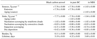
Table 4 Global mass budgets and lifetimes of total sea salt aerosol and total dust aerosol for the year-2000 MARC simulation, summed across the four dust aerosol modes and four sea salt aerosol modes. The processes acting as sources and sinks are summarised in Fig. 1d and e. Corresponding results for the year-1850 MARC simulation are shown in Table S4.

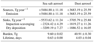
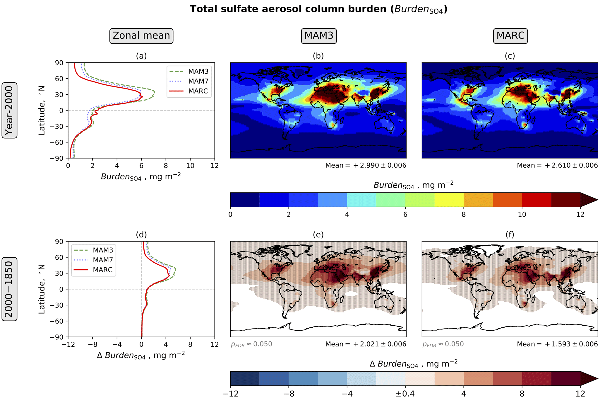
Figure 2 Annual mean total sulfate aerosol burden (Burden${}_{{\mathrm{SO}}_{\mathrm{4}}}$). For the zonal means (a, d), the standard errors, calculated using the annual zonal mean for each simulation year, are indicated by shading; however, this shading is not visible in Fig. 2, because the standard errors are smaller than the width of the plotted lines. For the maps (b, c, e, f), the area-weighted global mean and associated standard error, calculated using the annual global mean for each simulation year, are shown below each map. For the maps showing aerosol-induced 2000–1850 differences (e, f), white indicates differences with a magnitude less than the threshold value in the centre of the colour bar (±0.4 mg m⁻²). For locations where the magnitude is greater than this threshold value, stippling indicates differences that are statistically significant at a significance level of 0.05 after controlling the false discovery rate (Benjamini and Hochberg, 1995; Wilks, 2016); the two-tailed p values are generated by Welch's unequal variances t test, using annual mean data from each simulation year as the input; the approximate p value threshold, p_FDR, which takes the false discovery rate into account, is written below each map. The analysis period is 30 years. For MARC, the aerosol burdens (Figs. 2–6) have been calculated using monthly mass-mixing ratios.

Sea salt aerosol emissions, which are dependent on simulated wind speed and sea surface temperature, are approximately 5.5 Pg year⁻¹ in the MARC simulations (Tables 4 and S4); Liu et al. (2012) report slightly lower emissions of 5.0 Pg year⁻¹ for MAM. For MARC and MAM7, dry deposition is the largest sink of sea salt aerosol; for MAM3, wet deposition and dry deposition are approximately equal sinks. The sea salt aerosol lifetime is approximately 0.6 days for MARC and MAM7 and 0.8 days for MAM3.

Dust aerosol emissions, which are dependent on simulated wind speed and soil properties, are approximately 3.7 Pg year⁻¹ in the year-2000 MARC simulation (Table 4); Liu et al. (2012) report lower emissions of 3.1 Pg year⁻¹ for MAM3 and 2.9 Pg year⁻¹ for MAM7. For MARC, impaction scavenging and dry deposition play approximately equal roles in removing dust aerosol from the atmosphere; for MAM, dry deposition dominates. The dust aerosol lifetime is approximately 4 days for MARC and 3 days for MAM. The lifetime of dust in the year-1850 MARC simulation (Table S4) is very similar to that in the year-2000 simulation. However, dust emissions are slightly lower for the year-2000 simulation compared with the year-1850 simulation.

3.2 Aerosol column burdens

An aerosol column burden, also referred to as a loading, is the total mass of a given aerosol species in an atmospheric column. The advantage of column burdens is that they are relatively simple to understand, facilitating comparison between the different aerosol modules. However, when comparing the column burdens, it is important to remember that information about aerosol size distribution and the aerosol mixing state is hidden. Information about the vertical distribution is also hidden, because the burdens are integrated throughout the atmospheric column.

Figure 3 Annual mean total organic matter aerosol burden (Burden_OM) for MAM and total organic carbon aerosol burden (Burden_OC) for MARC. Due to different handling of organic carbon, MAM's Burden_OM is not directly equivalent to MARC's Burden_OC. Secondary organic aerosol from volatile organic compounds contributes to both Burden_OM and Burden_OC. The figure components are explained in the Fig. 2 caption.

3.2.1 Total sulfate aerosol burden

Figure 2a–c show the total sulfate aerosol burden (Burden${}_{{\mathrm{SO}}_{\mathrm{4}}}$) for the year-2000 simulations. For all three aerosol modules, year-2000 Burden${}_{{\mathrm{SO}}_{\mathrm{4}}}$ is highest in the Northern Hemisphere subtropics and midlatitudes, especially near source regions with high anthropogenic emissions of sulfur dioxide. Year-2000 Burden${}_{{\mathrm{SO}}_{\mathrm{4}}}$ is much lower in the Southern Hemisphere, especially over the remote Southern Ocean and Antarctica. In general, there is close agreement between MAM and MARC over the Northern Hemisphere tropics and the Southern Hemisphere. However, over the Northern Hemisphere subtropics, midlatitudes, and high latitudes, year-2000 Burden${}_{{\mathrm{SO}}_{\mathrm{4}}}$ is generally lower for MARC compared with MAM3. Interestingly, over the Northern Hemisphere subtropics, the zonal means are very similar between MAM7 and MARC. The differences between MARC, MAM3, and MAM7 may be due to differences in sulfate aerosol lifetime. However, it is not possible to test this conclusively; as pointed out in Sect. 3.1, the sulfate aerosol lifetimes diagnosed for MARC should not be directly compared to those diagnosed for MAM, because cloud cycling contributes to the sources and sinks of sulfate aerosol in MARC.

Figure 2d–f show $\mathrm{\Delta }{\text{Burden}}_{{\mathrm{SO}}_{\mathrm{4}}}$, the 2000–1850 difference in Burden${}_{{\mathrm{SO}}_{\mathrm{4}}}$. Both MAM3 and MARC produce widespread positive values of $\mathrm{\Delta }{\text{Burden}}_{{\mathrm{SO}}_{\mathrm{4}}}$ across the Northern Hemisphere and also across South America, Africa, and Oceania. For both MAM and MARC, global mean $\mathrm{\Delta }{\text{Burden}}_{{\mathrm{SO}}_{\mathrm{4}}}$ accounts for more than half of global mean year-2000 Burden${}_{{\mathrm{SO}}_{\mathrm{4}}}$, indicating that anthropogenic sulfur emissions are responsible for more than half of the global burden of sulfate aerosol.

3.2.2 Total organic matter and total organic carbon aerosol burdens

Figure 3a–c show the total organic matter aerosol burden (Burden_OM) for MAM and the total organic carbon aerosol burden (Burden_OC) for MARC for the year-2000 simulations. Due to different handling of organic carbon aerosol, MAM's Burden_OM is not directly equivalent to MARC's Burden_OC.

For both MAM3 and MARC, year-2000 Burden_OM and Burden_OC peak in the tropics, especially over sub-Saharan Africa and South America, due to emissions from wildfires. The impact of anthropogenic emissions of organic carbon aerosol is evident over South Asia and East Asia. Biogenic emissions of isoprene and monoterpene also contribute to Burden_OM and Burden_OC. Although the fields are not directly equivalent, it is interesting to note that MARC's Burden_OC is less than MAM's Burden_OM at latitudes with substantial emissions sources but greater than MAM's Burden_OM at high latitudes far from substantial emissions sources; this is consistent with the longer lifetime of MARC's organic carbon aerosol compared with MAM's organic matter and secondary organic aerosol.

Over the major emission regions of organic carbon aerosol, MAM3 and MARC generally produce positive values of ΔBurden_OM and ΔBurden_OC, the 2000–1850 differences in Burden_OM and Burden_OC (Fig. 3d–f). However, negative values of ΔBurden_OM and ΔBurden_OC are found over North America. These 2000–1850 differences arise due to changes in both wildfire emissions and anthropogenic emissions of organic carbon aerosol between year-1850 and year-2000. Although emissions of some volatile organic compounds do change between year-1850 and year-2000, emissions of isoprene and monoterpene remain unchanged, so these species are unlikely to contribute to ΔBurden_OM and ΔBurden_OC.

3.2.3 Total black carbon aerosol burden

Figure 4a–c show the total black carbon aerosol burden (Burden_BC) for the year-2000 simulations. For both MAM3 and MARC, year-2000 Burden_BC is high over sub-Saharan Africa and South America due to large emissions of black carbon aerosol from wildfires. However, the peak in zonal mean year-2000 Burden_BC occurs in the Northern Hemisphere subtropics and midlatitudes, due to anthropogenic emissions of black carbon aerosol over East Asia, South Asia, and Europe. Year-2000 Burden_BC for MARC is generally higher than that for MAM, especially over remote regions far away from sources. This is consistent with the longer lifetime of black carbon aerosol lifetime for MARC compared with MAM, likely due to the low hygroscopicity of MARC's pure black carbon aerosol mode.

MAM3 and MARC produce similar increases in Burden_BC between year-1850 and year-2000, as indicated by positive values of ΔBurden_BC (Fig. 4d–f). For MARC, positive values of ΔBurden_BC are found over even remote ocean regions, consistent with a longer black carbon lifetime for MARC compared with MAM3. Were it not for the decrease in MARC's black carbon aerosol lifetime between year-1850 (Table S3) and year-2000 (Table 3), ΔBurden_BC would be even larger.

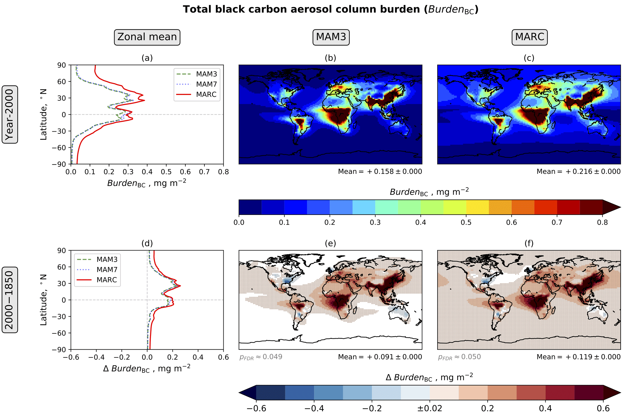
Figure 4 Annual mean total black carbon aerosol burden (Burden_BC). The figure components are explained in the Fig. 2 caption.

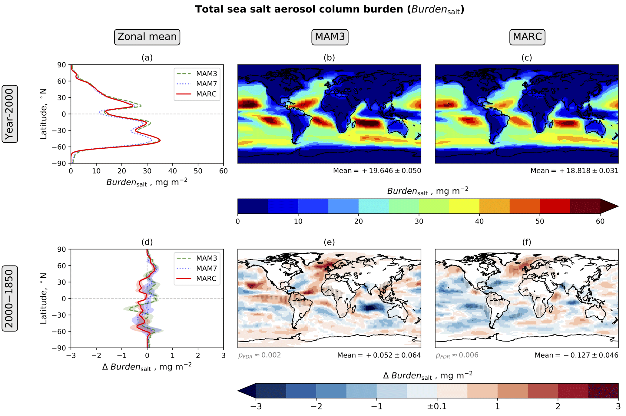
Figure 5 Annual mean total sea salt aerosol burden (Burden_salt). The figure components are explained in the Fig. 2 caption.

3.2.4 Total sea salt aerosol burden

Figure 5a–c show the total sea salt aerosol burden (Burden_salt) for the year-2000 simulations. For both MAM3 and MARC, year-2000 Burden_salt is highest over ocean areas with strong surface wind speeds (Fig. S9b, c). Over land, year-2000 Burden_salt is very low, due to the short lifetime of sea salt aerosol. Year-2000 Burden_salt is very similar between MAM3 and MARC. However, sea salt emissions and lifetime do vary slightly between MARC, MAM3, and MAM7, as noted in Sect. 3.1.

For both MAM3 and MARC, ΔBurden_salt, the 2000–1850 difference in Burden_salt (Fig. 5e, f), appears to be positively correlated with the aerosol-induced 2000–1850 difference in surface wind speeds (Fig. S9e, f). Changes in precipitation rate (Fig. S8e, f) likely also influence Burden_salt, because precipitation efficiently removes sea salt aerosol from the atmosphere. However, it should be noted that the aerosol-induced 2000–1850 differences in Burden_salt, surface wind speed, and precipitation rate are both relatively small and often statistically insignificant across most of the world. Hence these 2000–1850 differences may be due primarily to internal variability. If an interactive dynamical ocean were to be used, allowing SSTs to respond to the anthropogenic aerosol ERF, it is likely that we would find much larger aerosol-induced 2000–1850 differences in surface wind speed, the precipitation rate, and Burden_salt.

3.2.5 Total dust aerosol burden

Figure 6a–c show the total dust aerosol burden (Burden_dust) for the year-2000 simulations. Dust emissions primarily occur over desert areas, especially the Sahara, so year-2000 Burden_dust is highest directly over and downwind of these desert source regions. Year-2000 Burden_dust is much larger for MARC, which follows Albani et al. (2014), compared with MAM. The largest differences between MAM3 and MARC appear to occur directly over the desert source regions, suggesting that differences in dust emission drive the differences in year-2000 Burden_dust – if this is the case, dust emissions are far higher for MARC compared with MAM over the Sahara, Middle East, and East Asian deserts, while the opposite may be true over southern Africa and Australia. As mentioned in Sect. 3.1, global dust emissions are indeed higher for MARC compared with MAM. Differences in the lifetime of dust aerosol also contribute to the differences in year-2000 Burden_dust between MAM and MARC; the dust aerosol lifetime is 3 days for MAM and 4 days for MARC.

ΔBurden_dust, the aerosol-induced 2000–1850 difference in Burden_dust (Fig. 6d–f), reveals that Burden_dust decreases between the year-1850 and year-2000 simulations, especially over the Sahara. Both MAM3 and MARC produce a similar zonal mean decrease in Burden_dust. The reasons for the aerosol-induced 2000–1850 changes in Burden_dust are unclear, although changes in surface wind speed (Fig. S9d–f), which influence emissions, likely contribute; for MARC, global dust emissions are slightly lower in the year-2000 simulation (Table 4) compared to the year-1850 simulation (Table S4). As we noted above when discussing the sea salt burden, if an interactive dynamical ocean were to be used, it is likely that we would find much larger aerosol-induced 2000–1850 differences in surface wind speed, precipitation rate, and Burden_dust.

3.3 Aerosol–radiation interactions and the direct radiative effect

3.3.1 Aerosol optical depth

Aerosols scatter and absorb shortwave radiation, leading to the extinction of incoming solar radiation. Before considering the direct radiative effect, we first look at aerosol optical depth (AOD), a measure of the total extinction due to aerosols in an atmospheric column.

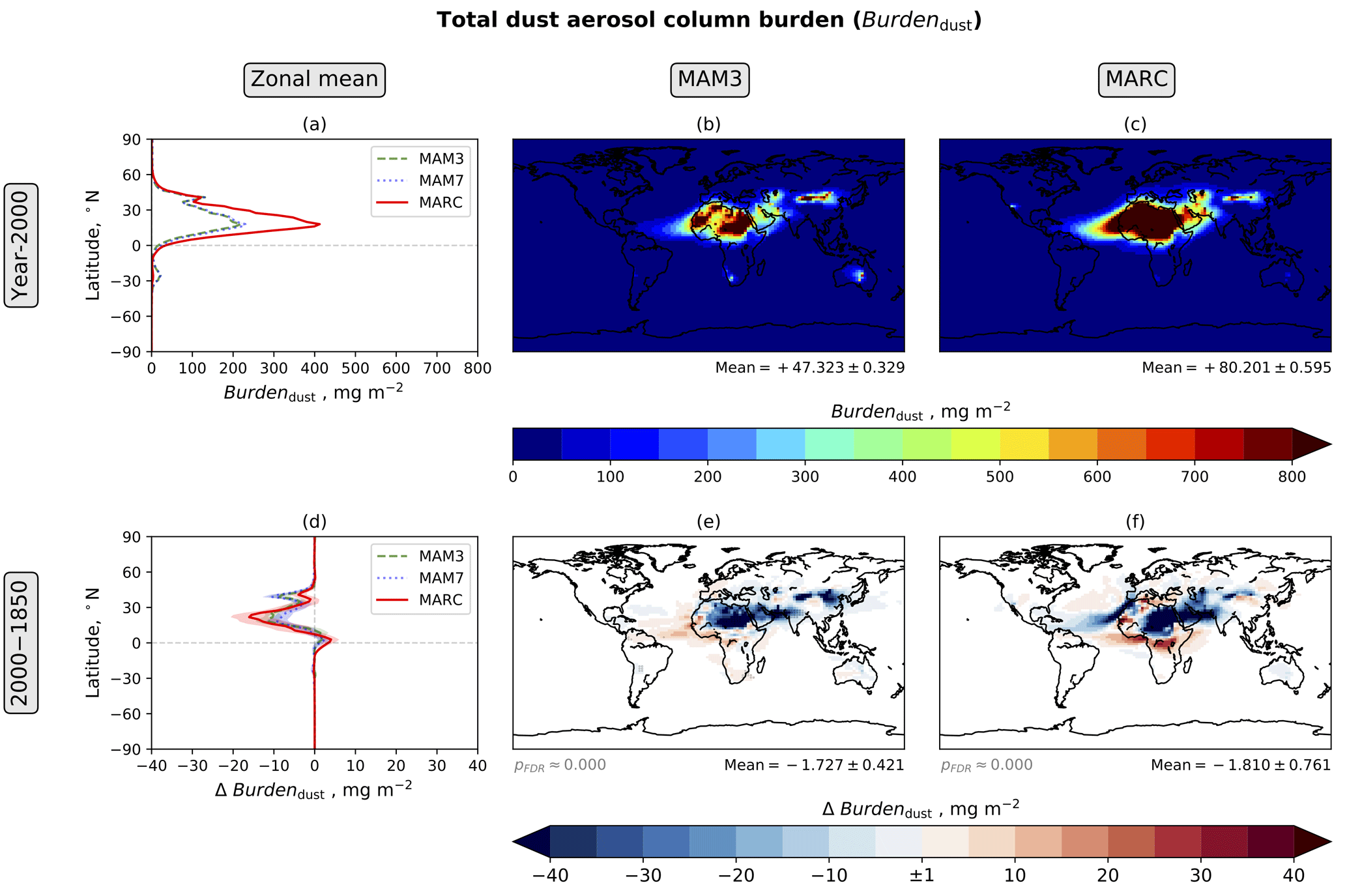
Figure 6 Annual mean dust aerosol burden (Burden_dust). The figure components are explained in the Fig. 2 caption.

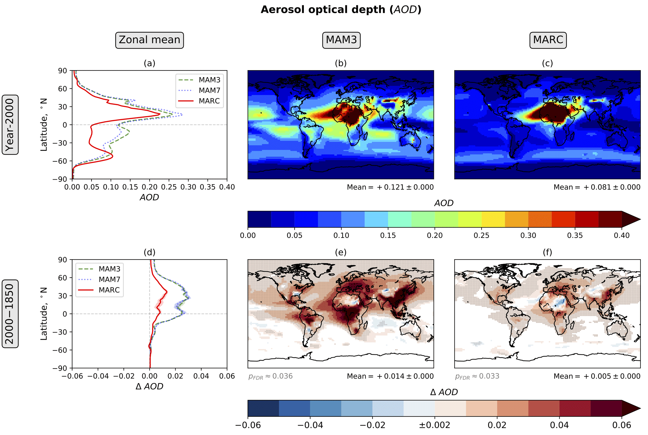
Figure 7 Annual mean aerosol optical depth (AOD). The figure components are explained in the Fig. 2 caption.

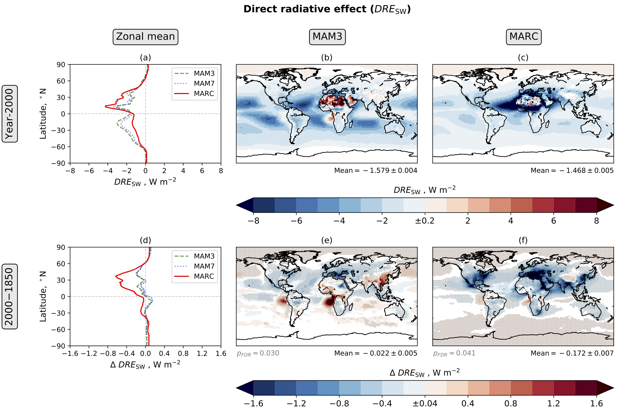
Figure 8 Annual mean direct radiative effect (DRE_SW; Eq. 3). The figure components are explained in the Fig. 2 caption. For all four maps, white indicates differences with a magnitude less than the threshold value in the centre of the corresponding colour bar.

Figure 7a–c show AOD for the year-2000 simulations. For both MAM and MARC, zonal mean year-2000 AOD peaks in the Northern Hemisphere subtropics, driven by the emission of dust from deserts, especially the Sahara. Over other regions, both anthropogenic aerosol emissions and natural aerosol emissions, including emissions of sea salt, contribute to year-2000 AOD. The year-2000 AOD values for MARC are often much lower than those for MAM3, especially over subtropical ocean regions. Rothenberg et al. (2018) have also previously noted that the AOD for MARC is generally lower than that retrieved from the MODerate Resolution Imaging Spectroradiometer (MODIS; Collection 5.1), but it should be noted that differences in spatial–temporal sampling (Schutgens et al., 2017, 2016) have not been accounted for, and satellite-based retrievals of AOD are not error-free.

The differences between the aerosol burdens for MAM and MARC, discussed above, are insufficient for explaining the differences in year-2000 AOD, especially the large difference in the Southern Hemisphere subtropics (where the burdens are similar between MAM and MARC). Hence it is likely that differences in the aerosol optical properties between MARC and MAM are responsible for the fact that MARC generally produces lower values of AOD. In particular, the large difference in year-2000 AOD between MAM3 and MARC over the subtropical ocean, where Burden_salt is large, is likely due to differences in the optical properties of sea salt aerosol.

Positive 2000–1850 differences in Burden${}_{{\mathrm{SO}}_{\mathrm{4}}}$, Burden_OM ∕ Burden_OC, and Burden_BC, discussed above, drive positive values of ΔAOD, the 2000–1850 difference in AOD (Fig. 7d–f). As was the case for year-2000 AOD, ΔAOD produced by MARC is generally much lower than ΔAOD produced by MAM3.

3.3.2 Direct radiative effect

Figure 8a–c show the direct radiative effect (DRE_SW) for the year-2000 simulations. DRE_SW reveals the influence of direct interactions between radiation and aerosols on the net shortwave flux at TOA (Eq. 3). Aerosols that scatter shortwave radiation efficiently, such as sulfate, generally contribute to negative values of DRE_SW, indicating a cooling effect on the climate system; aerosols that absorb shortwave radiation, such as black carbon, generally contribute to positive values of DRE_SW, indicating a warming effect on the climate system. Other factors, such as the presence of clouds, the vertical distribution of aerosols relative to clouds, and the albedo of the earth's surface, also play a role in determining DRE_SW (Stier et al., 2007). Due to these factors – especially the differing impact of scattering and absorbing aerosols and variations in the albedo of the earth's surface – large values of AOD may not necessarily correspond to large values of DRE_SW. Having said that, for both MAM3 and MARC, the regional distribution of year-2000 DRE_SW shares some similarities with that of year-2000 AOD. Over dark ocean surfaces in the subtropics, the scattering by aerosols drives negative values of year-2000 DRE_SW. The impact of dust on year-2000 DRE_SW differs between MAM3 and MARC, likely due to differing optical properties. For MAM3, the absorption by dust drives positive values over the bright surface of the Sahara, while little radiative impact is evident downwind over the dark surface of the tropical Atlantic Ocean; for MARC, the scattering by dust drives negative values over the tropical Atlantic Ocean, while little radiative impact is evident over the Sahara. The impact of black carbon aerosol on year-2000 DRE_SW also differs between MAM3 and MARC. For MAM3, absorption by black carbon aerosol drives positive values of DRE_SW over the South Atlantic stratocumulus deck near southern Africa; for MARC, negative values of DRE_SW are found over the stratocumulus deck, suggesting a weaker absorption by black carbon aerosol compared with MAM3. The differing absorption is likely due to the differing representations of the aerosol mixing state and associated optical properties; the majority of MARC's black carbon aerosol is found in the pure BC mode, whereas MAM's black carbon aerosol is internally mixed with other species, likely leading to stronger absorption for MAM compared with MARC.

For MAM, ΔDRE_SW, the 2000–1850 difference in DRE_SW, is relatively weak at all latitudes (Fig. 8d, e), with a global mean of only $-\mathrm{0.02}\pm \mathrm{0.01}$ W m⁻² for MAM3 and $-\mathrm{0.00}\pm \mathrm{0.01}$ W m⁻² for MAM7 (Table 5), due to the cooling effect of anthropogenic sulfur emissions being offset by the warming effect of increased black carbon aerosol emissions (Ghan et al., 2012). In contrast, for MARC, ΔDRE_SW reveals a relatively strong cooling effect across much of the Northern Hemisphere (Fig. 8d, f), especially near anthropogenic sources of sulfur emissions, leading to a global mean ΔDRE_SW of $-\mathrm{0.17}\pm \mathrm{0.01}$ W m⁻².

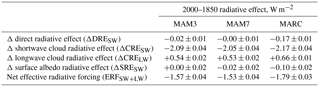
Table 5 Area-weighted global mean radiative effects. Combined standard errors are calculated using the annual global mean for each simulation year. The regional distributions of these radiative effects are shown in Figs. 8, 14, 15, 16, and 17. ERF_SW+LW is the sum of the other radiative effect components.

3.3.3 Absorption by aerosols in the atmosphere

Figure 9a–c show the absorption of shortwave radiation by aerosols in the atmosphere (AAA_SW; Eq. 8) for the year-2000 simulations. The consideration of AAA_SW, which reveals heating of the atmosphere by aerosols, complements the consideration of DRE_SW. For example, over the Sahara, we noted above that the dust aerosol in MARC exerts only a weak direct radiative effect at TOA (Fig. 8c); however, Fig. 9c reveals that the dust aerosol in MARC leads to the strong heating of the atmosphere. For both MAM and MARC, year-2000 AAA_SW is largest near emission sources of dust, especially over the Sahara where year-2000 Burden_dust is particularly high, showing that dust is the primary driver of year-2000 AAA_SW. Further away from the dust emission source regions, year-2000 AAA_SW is spatially correlated with year-2000 Burden_BC, showing that black carbon aerosol also contributes to year-2000 AAA_SW. Despite the fact that year-2000 Burden_dust and Burden_BC are larger for MARC compared with MAM, year-2000 AAA_SW is generally weaker for MARC compared with MAM; the weaker absorption for MARC is likely due to differences in the aerosol optical properties associated with the different handling of dust and black carbon aerosol mixing state between MAM and MARC.

ΔAAA_SW, the 2000–1850 difference in AAA_SW (Fig. 9d–f), generally follows the same regional distribution as ΔBurden_BC, showing that changes in emissions of black carbon aerosol dominate ΔAAA_SW. Although dust dominates year-2000 AAA_SW, changes in dust emissions exert only a relatively small influence on ΔAAA_SW. As with year-2000 AAA_SW, ΔAAA_SW is generally weaker for MARC compared with MAM3.

The absorption of shortwave radiation by aerosols can drive rapid adjustments of the atmosphere, such as changes to atmospheric stability and humidity, influencing clouds (Stjern et al., 2017). Such “semi-direct” effects may contribute to the cloud radiative effects discussed below. However, Ghan et al. (2012) found both the shortwave and longwave semi-direct radiative effects to be statistically insignificant for MAM3 and MAM7; we expect the same to apply for MARC, because the default CAM5.3 cloud microphysics scheme is also used. Cloud microphysical effects dominate the cloud radiative effects.

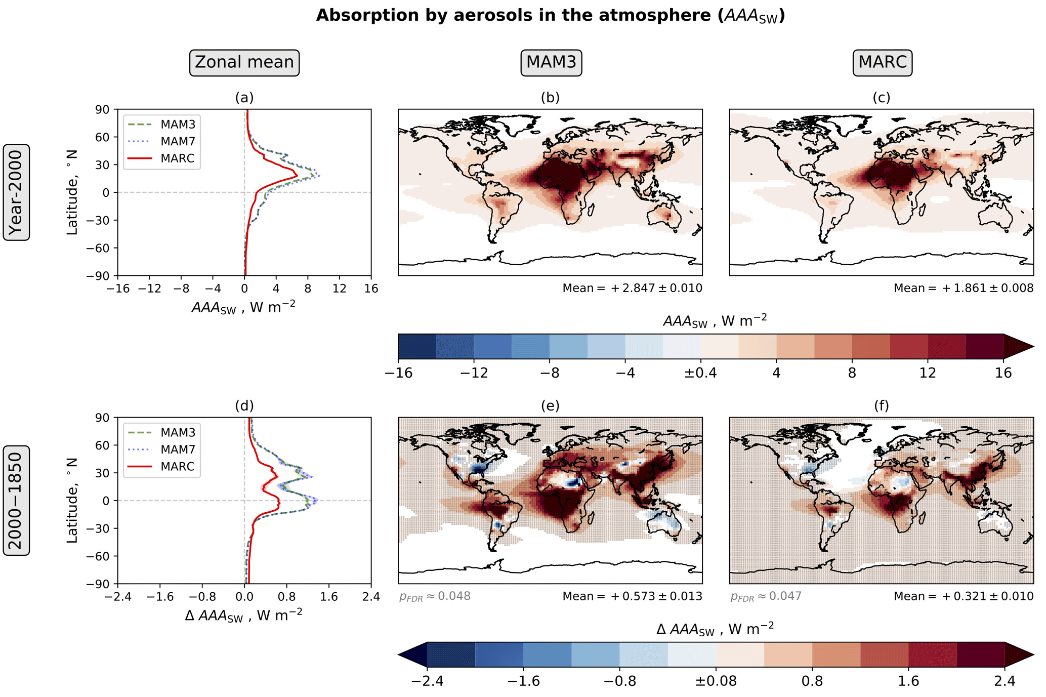
Figure 9 Annual mean absorption by aerosols in the atmosphere (AAA_SW; Eq. 8). The figure components are explained in the Fig. 2 caption. For all four maps, white indicates differences with a magnitude less than the threshold value in the centre of the corresponding colour bar.

Figure 10 Annual mean cloud condensation nuclei concentration at 0.1 % supersaturation (CCN_conc) in model level 24 (in the lower troposphere). The figure components are explained in the Fig. 2 caption. Corresponding results showing CCN_conc near the surface and in the mid-troposphere are shown in Figs. S1 and S2.

3.4 Aerosol–cloud interactions and the cloud radiative effects

3.4.1 Cloud condensation nuclei concentration

Many aerosol particles have the potential to become the cloud condensation nuclei (CCN) on which water vapour condenses to form cloud droplets. Figure 10a–c show the CCN concentration at a fixed supersaturation of 0.1 % (CCN_conc) in the lower troposphere for the year-2000 simulations. Corresponding results showing year-2000 CCN_conc near the surface and in the mid-troposphere are shown in Figs. S1a–c and S2a–c in the Supplement. Looking at year-2000 CCN_conc across these different vertical levels, we make two initial observations. First, for both MAM and MARC, year-2000 CCN_conc is generally higher in the Northern Hemisphere; second, year-2000 CCN_conc is generally much lower for MARC compared with MAM.

When we look in more detail at the regional distribution of year-2000 CCN_conc for MAM3 and compare this to the column burden results, we notice that locations with high CCN_conc have either high Burden${}_{{\mathrm{SO}}_{\mathrm{4}}}$ or high Burden_OM. This suggests that, for MAM3, the organic matter aerosol – internally mixed with other species with high hygroscopicity – contributes to efficient CCN, consistent with two previous MAM3-based studies that found that organic carbon emissions from wildfires can exert a strong influence on clouds (Grandey et al., 2016a; Jiang et al., 2016).

In contrast, for MARC, the regional distribution of year-2000 CCN_conc closely resembles that of Burden${}_{{\mathrm{SO}}_{\mathrm{4}}}$ but does not resemble that of Burden_OC. This suggests that, for MARC, the organic carbon aerosol – much of which remains in a pure organic carbon aerosol mode with very low hygroscopicity – is not an efficient source of CCN.

If we look at the results for ΔCCN_conc, the 2000–1850 difference in CCN_conc (Figs. 10d–f, S1d–f, and S2d–f), similar deductions about sulfate aerosol and organic carbon aerosol can be made as were made above. For MAM3, the regional distribution of ΔCCN_conc reveals that changes in the availability of CCN are associated with both $\mathrm{\Delta }{\text{Burden}}_{{\mathrm{SO}}_{\mathrm{4}}}$ and ΔBurden_OM. For MARC, the regional distribution of ΔCCN_conc is associated with $\mathrm{\Delta }{\text{Burden}}_{{\mathrm{SO}}_{\mathrm{4}}}$, but it is not closely associated with ΔBurden_OC.

For both MAM and MARC, ΔCCN_conc is generally positive, revealing increasing availability of CCN between year-1850 and year-2000. The absolute increase is smaller for MARC than for MAM. However, the percentage increase is larger for MARC than for MAM.

It is important to note that these CCN_conc results are for a fixed supersaturation of 0.1 %, but as pointed out by Rothenberg et al. (2018) “all aerosol [particles] are potentially CCN, given an updraft sufficient enough in strength to drive a high-enough supersaturation such that they grow large enough to activate”. Furthermore, the number of CCN that are actually activated is influenced by competition for water vapour among various types of aerosol particles, which depends on the details of the aerosol population, including size distribution and mixing state. When aerosol particles with a lower hygroscopicity rise alongside aerosol particles with a higher hygroscopicity in a rising air parcel, the latter would normally be activated first at a supersaturation that is much lower than the one required for the former to become activated; the consequent condensation of water vapour to support the diffusive growth of the newly formed cloud particles would effectively lower the saturation level of the air parcel and further reduce the chance for the lower hygroscopicity aerosol particles to be activated (Rothenberg and Wang, 2016, 2017). In other words, CCN_conc at a fixed supersaturation is not necessarily a good indicator of the number of CCN that are actually activated, because activation depends on specific environmental conditions and the details of the aerosol population present.

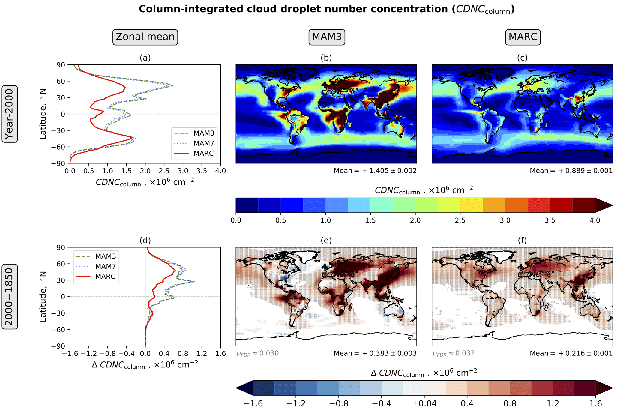
Figure 11 Annual mean column-integrated cloud droplet number concentration (CDNC_column). The figure components are explained in the Fig. 2 caption.

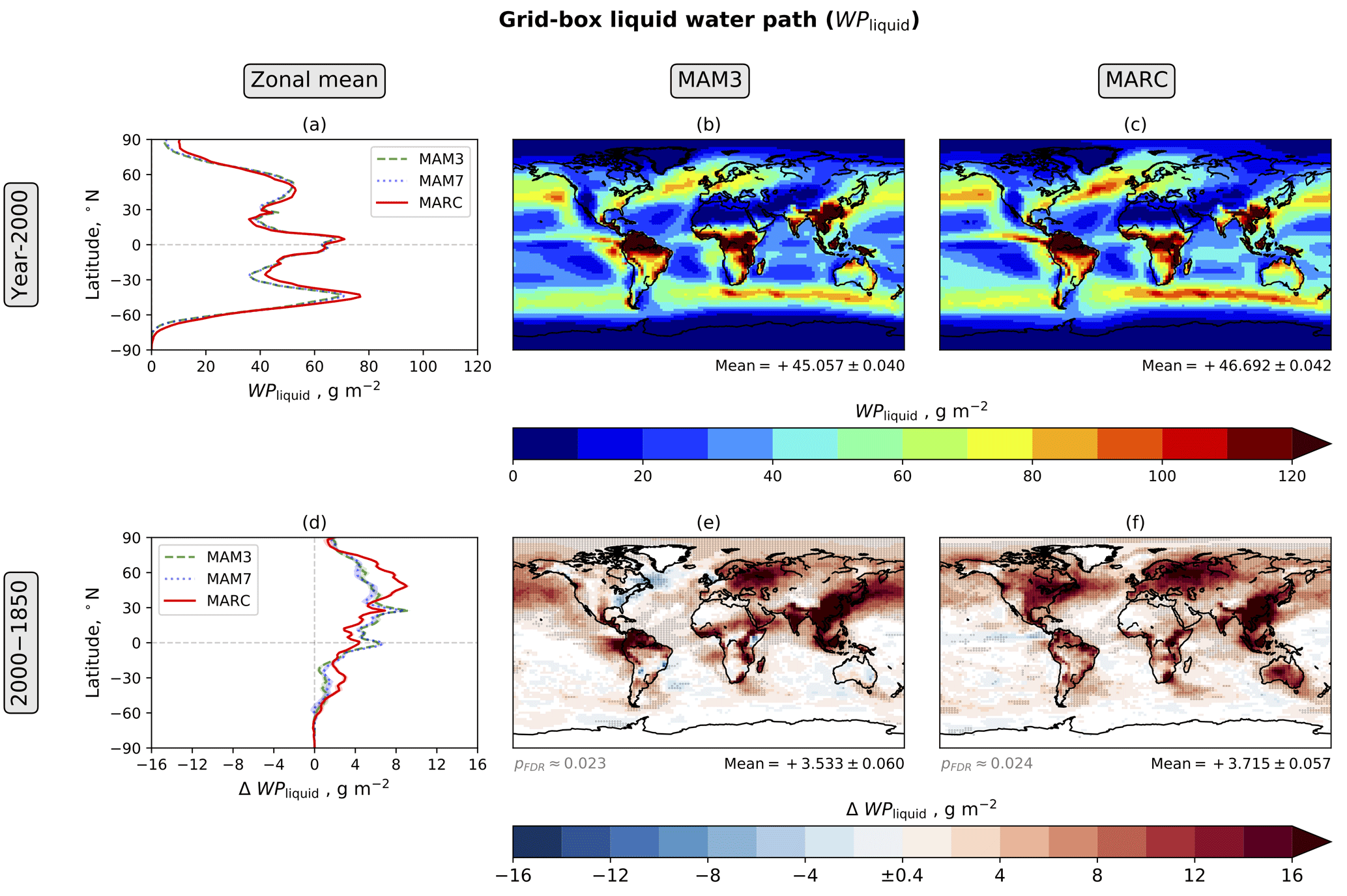
Figure 12 Annual mean grid-box cloud liquid water path (WP_liquid). The figure components are explained in the Fig. 2 caption.

Differences in the representation of the aerosol mixing state and hygroscopicity may lead to large differences in aerosol-activation spectra. In an aerosol model such as MAM that includes only internally mixed modes, the hygroscopicity of a given mode is derived by volume weighting through all the included aerosol species and is therefore not very sensitive to changes in the chemical composition of the mode. In contrast, MARC explicitly handles the mixing state and thus the hygroscopicity of each individual type of aerosol; for example, the hygroscopicity of the pure OC and pure BC modes is very low, the hygroscopicity of the MOS mode depends on the internal mixing state of organic carbon and sulfate (assuming homogeneous mixing), and the hygroscopicity of the MBS mode is as high as that of pure sulfate (assuming a core-shell model; Rothenberg et al., 2018).

3.4.2 Column-integrated cloud droplet number concentration

The availability of CCN influences cloud microphysics via the formation of cloud droplets. Figure 11a–c show the column-integrated cloud droplet number concentration (CDNC_column) for the year-2000 simulations. For MAM, year-2000 CDNC_column is generally higher in the Northern Hemisphere, with very high values occurring over regions with abundant sulfate aerosol or organic carbon aerosol that provide abundant CCN. In contrast, for MARC there is no strong inter-hemispheric asymmetry in year-2000 CDNC_column; there appears to be no influence from organic carbon aerosol, consistent with the CCN_conc results discussed above, and the influence of sulfate aerosol appears weaker than for MAM.

No global observations of CDNC_column exist. However, satellite-based estimates of the cloud-top cloud droplet number concentration (CDNC_top) can be derived using the adiabatic assumption, although the uncertainties are large. MARC tends to underestimate CDNC_top compared to MODIS-derived estimates (Rothenberg et al., 2018).

When we look at ΔCDNC_column, the 2000–1850 difference in CDNC_column (Fig. 11d–f), we see that anthropogenic emissions generally drive increases in CDNC_column, as expected. The absolute increase is smaller for MARC than for MAM. However, the percentage increase is comparable between MARC and MAM. As was the case for ΔCCN_conc, for MAM3, the regional distribution of ΔCDNC_column appears to be associated with both $\mathrm{\Delta }{\text{Burden}}_{{\mathrm{SO}}_{\mathrm{4}}}$ and ΔBurden_OM, whereas for MARC, the regional distribution of ΔCDNC_column is associated with $\mathrm{\Delta }{\text{Burden}}_{{\mathrm{SO}}_{\mathrm{4}}}$ but is not closely associated with ΔBurden_OC.

3.4.3 Grid-box cloud liquid and cloud ice water paths

In addition to influencing cloud microphysical properties (such as cloud droplet number concentration), the availability of CCN and ice nuclei influence cloud macrophysical properties (such as cloud water path). Figure 12a–c show the grid-box cloud liquid water path (WP_liquid) for the year-2000 simulations. Year-2000 WP_liquid is highest in the tropics and midlatitudes. The regional distribution of year-2000 WP_liquid is similar to that of total cloud fractional coverage (Fig. S4a–c). The regional distribution of year-2000 WP_liquid for MARC is very similar to that for MAM. However, compared with MAM, MARC produces slightly higher year-2000 WP_liquid in the Southern Hemisphere midlatitudes, the Southern Hemisphere subtropics, and the Arctic.

Figure 13a–c show the grid-box cloud ice water path (WP_ice) for the year-2000 simulations. As with WP_liquid, year-2000 WP_ice is highest in the tropics and midlatitudes. The regional distribution of year-2000 WP_ice is similar to that of high-level cloud fractional coverage (Fig. S7a–c), and is similar between MAM and MARC. However, year-2000 WP_ice is consistently lower for MARC than for MAM. Although MARC and MAM3 are coupled to the same ice and mixed-phase cloud microphysics scheme (Gettelman et al., 2010; Liu et al., 2007), differences in the availability of ice nuclei can arise due to differences in dust and sulfate number concentrations and size distributions. The uncertainties associated with ice nucleation are very large (Garimella et al., 2018).

The 2000–1850 differences in WP_liquid and WP_ice are shown in Figs. 12d–f and 13d–f. MAM3 produces large increases in WP_liquid over Europe, East Asia, Southeast Asia, South Asia, parts of Africa, and northern South America – the regional distribution of ΔWP_liquid is similar to the regional distributions of ΔCCN_conc and ΔCDNC_column. MARC produces large increases in WP_liquid over the same regions, and additionally over Australia and North America. ΔWP_liquid is often larger for MARC than for MAM3, especially over the Northern Hemisphere midlatitudes. For MARC, in comparison with MAM3, the relatively strong ΔWP_liquid response is consistent with the relatively strong percentage change in ΔCCN_conc.

Globally, for both MAM3 and MARC, the ΔWP_ice response is relatively weak (Fig. 13d–f). However, relatively large values of ΔWP_ice, both positive and negative, are found regionally. This regional response differs between MAM3 and MARC. For both MAM3 and MARC, it appears that decreases in WP_ice correspond to increases in Burden_OM and Burden_OC (Fig. 3e, f), but this relationship is likely spurious, because organic carbon aerosol does not directly influence ice processes in either aerosol module.

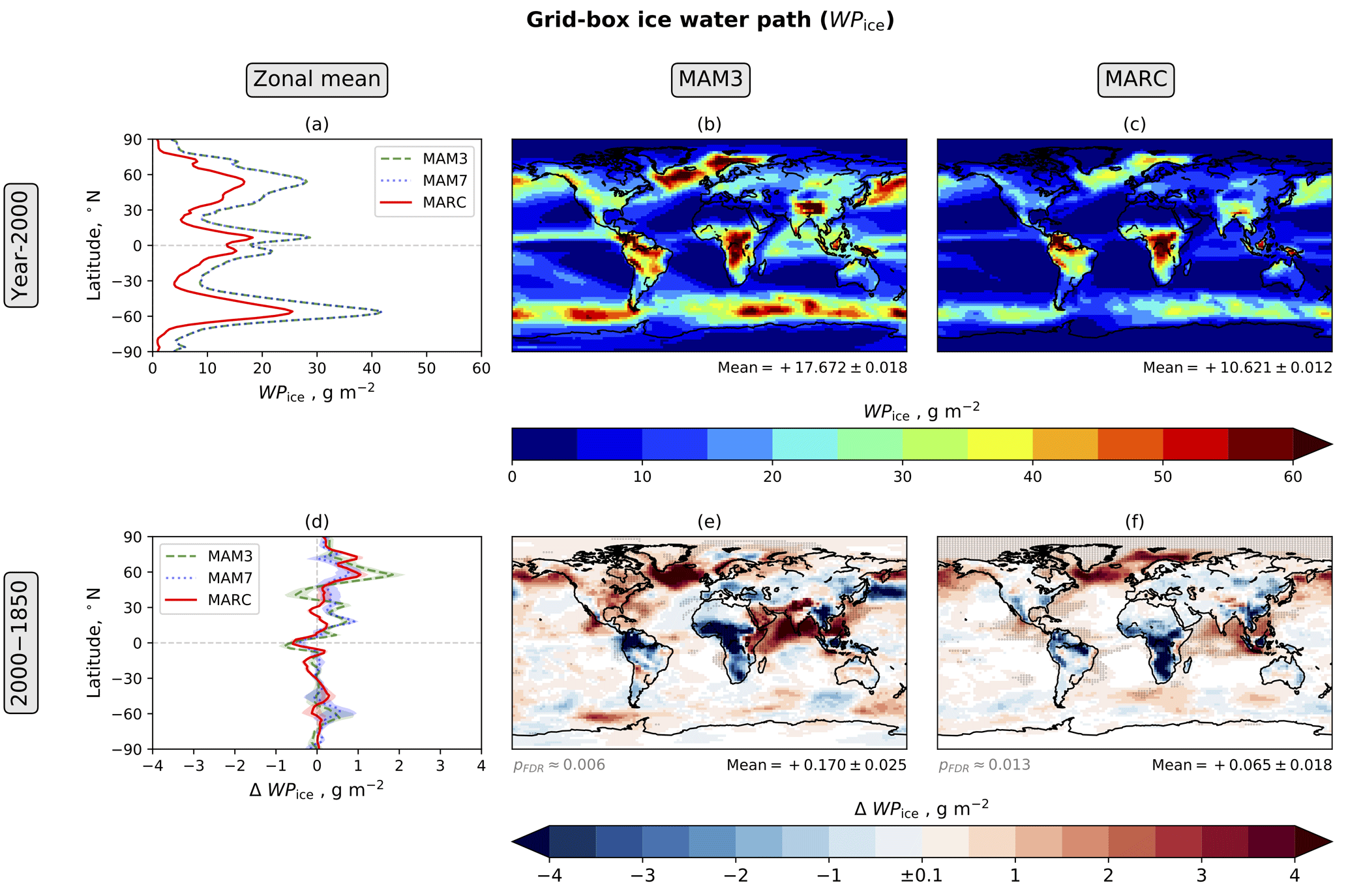
Figure 13 Annual mean grid-box cloud ice water path (WP_ice). The figure components are explained in the Fig. 2 caption.

3.4.4 Shortwave cloud radiative effect

Figure 14a–c show the clean-sky shortwave cloud radiative effect (CRE_SW; Eq. 4) for the year-2000 simulations. Clouds scatter much of the incoming solar radiation, exerting a strong cooling effect on the climate system. Globally, year-2000 CRE_SW is −53.9 W m⁻² for MAM3 and −52.2 W m⁻² for MARC. For both MAM and MARC, CRE_SW is strongest in the tropics and midlatitudes. The regional distribution of year-2000 CRE_SW is negatively correlated with WP_liquid and WP_total (the total cloud water path; Fig. S3); large values of WP_liquid and WP_total correspond to a strong cooling effect.

The same applies to ΔCRE_SW, the 2000–1850 difference in CRE_SW (Fig.  14d–f), which is negatively correlated with ΔWP_liquid and ΔWP_total; increases in WP_liquid and WP_total drive a stronger shortwave cloud cooling effect. For both MAM3 and MARC, the cooling effect of ΔCRE_SW is strongest in the Northern Hemisphere, particularly over regions with high anthropogenic sulfur emissions, especially East Asia, Southeast Asia, and South Asia. Compared with MAM, MARC produces a slightly stronger ΔCRE_SW response in the Northern Hemisphere midlatitudes and a slightly weaker ΔCRE_SW response in the Northern Hemisphere subtropics. Another difference between MAM3 and MARC is the land–ocean contrast: compared with MAM3, MARC often produces a slightly stronger ΔCRE_SW response over land but a weaker ΔCRE_SW response over the ocean. In particular, MARC produces a weaker ΔCRE_SW response over the stratocumulus decks near South America and southern Africa, likely because organic carbon aerosol is not an efficient source of CCN in MARC.

When globally averaged, the global mean ΔCRE_SW for MARC ($-\mathrm{2.17}\pm \mathrm{0.04}$ W m⁻²) is stronger than that for MAM3 ($-\mathrm{2.09}\pm \mathrm{0.04}$ W m⁻²) and MAM7 ($-\mathrm{2.05}\pm \mathrm{0.04}$ W m⁻²). The stronger ΔCRE_SW response for MARC is consistent with the larger percentage change in ΔCCN_conc for MARC compared with MAM.

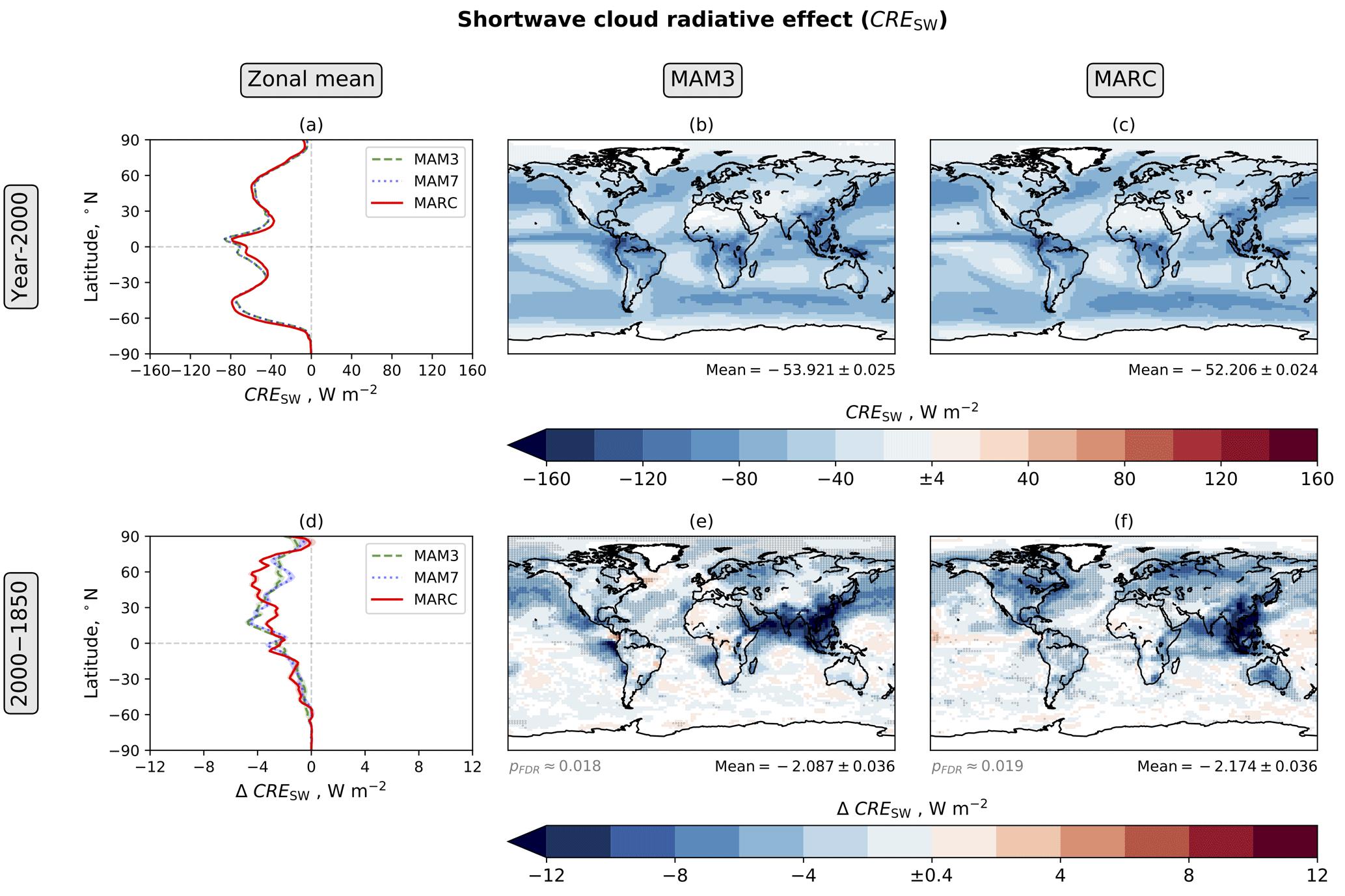
Figure 14 Annual mean clean-sky shortwave cloud radiative effect (CRE_SW; Eq. 4). The figure components are explained in the Fig. 2 caption. For all four maps, white indicates differences with a magnitude less than the threshold value in the centre of the corresponding colour bar.

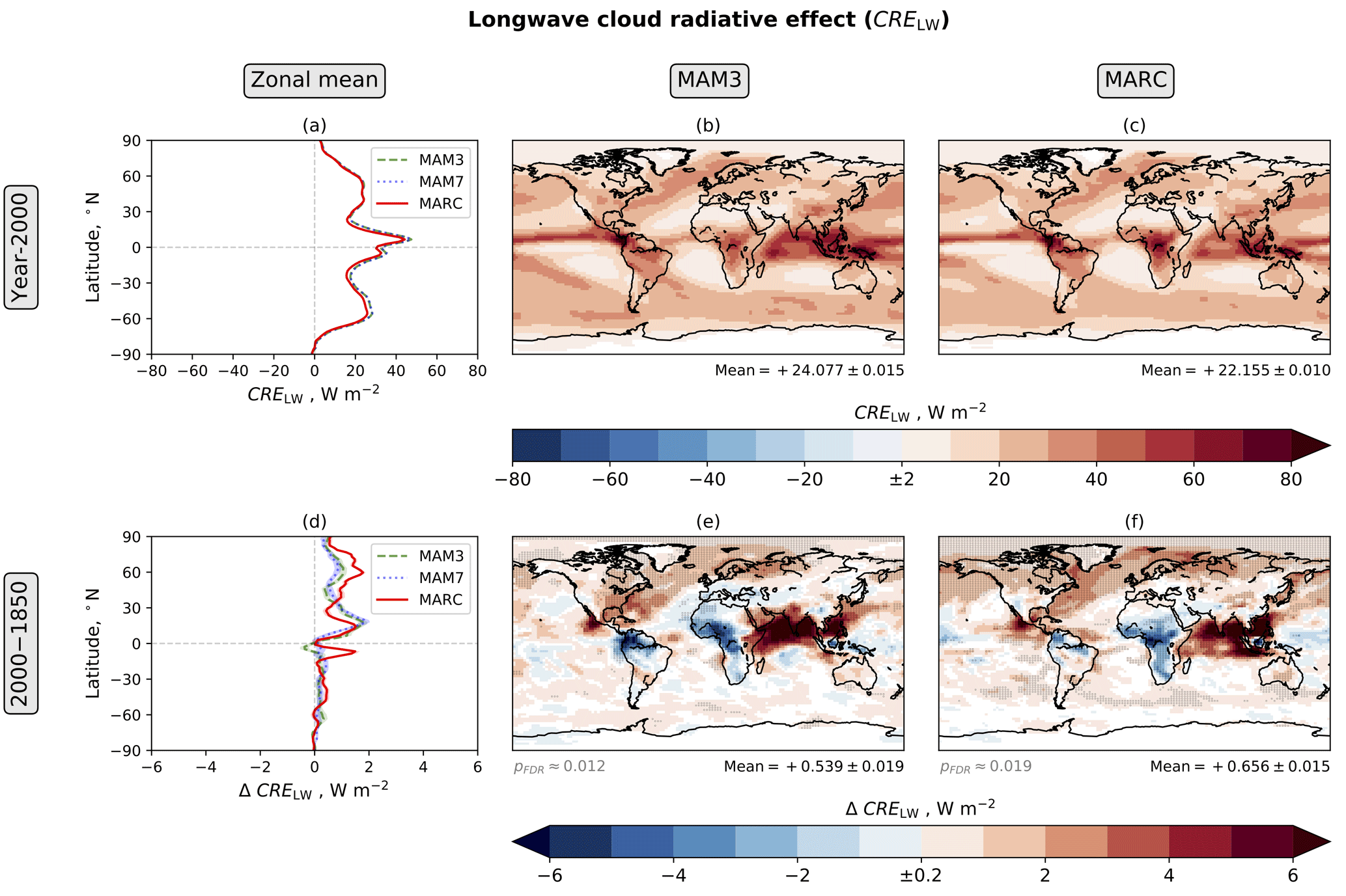
Figure 15 Annual mean longwave cloud radiative effect (CRE_LW; Eq. 6). The figure components are explained in the Fig. 2 caption. For all four maps, white indicates differences with a magnitude less than the threshold value in the centre of the corresponding colour bar.

Figure 16 Annual mean aerosol-induced 2000–1850 surface albedo radiative effect (ΔSRE_SW; Eq. 5). The figure components are explained in the Fig. 2 caption.

Figure 17 Annual mean 2000–1850 net effective radiative forcing (ERF_SW+LW; Eq. 7). The figure components are explained in the Fig. 2 caption. When comparing the relative contributions of the different radiative effect components to ERF_SW+LW, note that different colour bars are used in Figs. 8, 14, 15, and 16.

3.4.5 Longwave cloud radiative effect

The cooling effect of CRE_SW is partially offset by the warming effect of CRE_LW, the longwave cloud radiative effect that arises due to absorption of longwave thermal infrared radiation (Eq. 6). Figure 15a–c show CRE_LW for the year-2000 simulations. Globally, year-2000 CRE_LW is +24.1 W m⁻² for MAM3 and +22.2 W m⁻² for MARC. As with the shortwave cooling effect, the longwave warming effect is strongest in the tropics and midlatitudes, for both MAM and MARC. The regional distribution of year-2000 CRE_LW is positively correlated with WP_ice (Fig. 13a–c) and the high-level cloud fraction (Fig. S7a–c) – high-level ice cloud drives the longwave warming effect.

The same is true for ΔCRE_LW, the 2000–1850 difference in CRE_LW (Fig. 15d–f); changes in high-level ice cloud cover drive changes in the longwave cloud warming effect. For both MAM3 and MARC, ΔCRE_LW is positive over much of Southeast Asia, South Asia, the Indian Ocean, the Atlantic Ocean, and the Pacific Ocean; ΔCRE_LW is negative over much of Africa and parts of South America. MAM3 produces a global mean ΔCRE_LW of $+\mathrm{0.54}\pm \mathrm{0.02}$ W m⁻², and MAM7 produces a global mean ΔCRE_LW of $+\mathrm{0.53}\pm \mathrm{0.02}$ W m⁻², while MARC produces a stronger global mean of $+\mathrm{0.66}\pm \mathrm{0.01}$ W m⁻². Hence ΔCRE_LW offsets approximately one quarter to one third of the ΔCRE_SW cooling effect.

3.5 The surface albedo radiative effect

In addition to interacting with radiation both directly and indirectly via clouds, aerosols can influence the earth's radiative energy balance via changes to the surface albedo. The surface albedo radiative effect (ΔSRE_SW; Eq. 5), “includes effects of both changes in snow albedo due to deposition of absorbing aerosol, and changes in snow cover induced by deposition and by the other aerosol forcing mechanisms” (Ghan, 2013). For both MAM3 and MARC, the deposition of absorbing aerosol is enabled via the coupling between CAM5 and the land scheme in CESM, and “other aerosol forcing mechanisms” include aerosol-induced changes in precipitation rate. Aerosol-induced changes in column water vapour can also influence the calculation of ΔSRE_SW, because F_{clean, clear} is sensitive to near-infrared absorption by water vapour, but the contribution from such changes in column water vapour is small. (ΔSRE_SW does not include changes in land use, because the only difference between the year-1850 and year-2000 simulations is the aerosol emissions.)

Figure 16 shows ΔSRE_SW, the aerosol-induced 2000–1850 surface albedo radiative effect. In the Arctic and high-latitude land regions of the Northern Hemisphere, ΔSRE_SW can be relatively large. MAM3 produces a mixture of positive and negative ΔSRE_SW values, averaging out to zero globally ($+\mathrm{0.00}\pm \mathrm{0.02}$ W m⁻²). However, MARC tends to produce mainly negative ΔSRE_SW values, averaging out to a global mean of $-\mathrm{0.10}\pm \mathrm{0.02}$ W m⁻².

The ΔSRE_SW response is associated with aerosol-induced 2000–1850 changes in snow cover over both land and sea-ice (Fig. S10d–f); increases in snow cover lead to negative ΔSRE_SW values, while decreases in snow cover lead to positive ΔSRE_SW values. Changes in snow rate (Fig. S11d–f) likely play a major role, explaining much of the snow cover response. Changes in black carbon deposition (Fig. S12d–f), contributing to changes in the mass of black carbon in the top layer of snow (Fig. S13d–f), may also play a role. The mass of black carbon in the top layer of snow is much lower for MARC compared with MAM3 (Fig. S13a–c), likely due to differences in dry deposition of black carbon; the rate of dry deposition of black carbon aerosol is 0.42 Tg year⁻¹ in MARC (Table 3), much lower than the rate of 1.27 Tg year⁻¹ in MAM3 (Liu et al., 2012). The aerosol-induced 2000–1850 difference in the mass of black carbon in the top layer of snow is also much lower for MARC compared with MAM3 (Fig. S13d–f).

3.6 Net effective radiative forcing

The net effective radiative forcing (ERF_SW+LW) – the 2000–1850 difference in the net radiative flux at TOA (Eq. 7) – is effectively the sum of the radiative effect components we discussed above. Figure 17 shows ERF_SW+LW; Table 5 summarises the global mean contribution from the different radiative effect components.

In general, the cloud shortwave component, ΔCRE_SW, dominates, resulting in negative values of ERF_SW+LW across much of the world. In particular, strongly negative values of ERF_SW+LW, indicating a large cooling effect, are found near regions with substantial anthropogenic sulfur emissions. The cooling effect is far stronger in the Northern Hemisphere than it is in the Southern Hemisphere. If coupled atmosphere–ocean simulations were to be performed, allowing SSTs to respond, the large inter-hemispheric difference in ERF_SW+LW would likely impact inter-hemispheric temperature gradients and hence rainfall patterns (Chiang and Friedman, 2012; Grandey et al., 2016b; Wang, 2015).

Across much of the globe, the net cooling effect of ERF_SW+LW produced by MARC is similar to that produced by MAM. However, in the midlatitudes, MARC produces a stronger net cooling effect, especially over North America, Europe, and northern Asia. Another difference is that MARC appears to exert more widespread cooling over land than MAM3 does, while the opposite appears to be the case over the ocean. These differences in the regional distribution of ERF_SW+LW are largely due to differences in the regional distribution of ΔCRE_SW. As mentioned in the previous paragraph, rainfall patterns are sensitive to changes in surface temperature gradients. Therefore, if SSTs were allowed to respond to the forcing, the differences in the regional distribution of ERF_SW+LW between MARC and MAM may drive differences in rainfall patterns.

When averaged globally, MAM3 produces a global mean ERF_SW+LW of $-\mathrm{1.57}\pm \mathrm{0.04}$ W m⁻², and MAM7 produces a global mean ERF_SW+LW of $-\mathrm{1.53}\pm \mathrm{0.04}$ W m⁻²; MARC produces a stronger global mean ERF_SW+LW of $-\mathrm{1.79}\pm \mathrm{0.03}$ W m⁻². The ERF_SW+LW produced by CAM5.3-MARC-ARG is particularly strong compared with many other global climate models (Shindell et al., 2013).

4 Summary and conclusions

The specific representation of aerosols in global climate models, especially the representation of the aerosol mixing state, has important implications for aerosol hygroscopicity, aerosol lifetime, aerosol column burdens, aerosol optical properties, and cloud condensation nuclei (CCN) availability. For example, in addition to internally mixed modes, MARC also includes a pure organic carbon aerosol mode and a pure black carbon aerosol mode, both of which have very low hygroscopicity. The low hygroscopicity of these pure organic carbon and pure black carbon modes leads to increased lifetimes of total organic carbon aerosol and total black carbon aerosol, influencing aerosol column burdens. Furthermore, the representation of the aerosol mixing state and the associated implications for hygroscopicity strongly influence the ability of the aerosol particles to act as CCN. For example, MARC's organic carbon aerosol is not an efficient source of CCN, but MAM's organic matter aerosol – internally mixed with other species with high hygroscopicity – is an efficient source of CCN.

We have demonstrated that changing the aerosol module in CAM5.3 influences both the direct and indirect radiative effects of aerosols. Standard CAM5.3, which uses the MAM3 aerosol module, produces a global mean net ERF of $-\mathrm{1.57}\pm \mathrm{0.04}$ W m⁻² associated with the 2000–1850 difference in aerosol (including aerosol precursor) emissions; CAM5.3-MARC-ARG, which uses the MARC aerosol module, produces a stronger global mean net ERF of $-\mathrm{1.79}\pm \mathrm{0.03}$ W m⁻², a particularly strong cooling effect compared with other climate models (Shindell et al., 2013). For MARC compared with MAM, the stronger global mean net ERF can be attributed to stronger cooling via the direct radiative effect, the shortwave cloud radiative effect, and the surface albedo radiative effect, as summarised below. Furthermore, differences in the regional distribution of the shortwave cloud radiative effect drive differences in the regional distribution of net ERF.

By analysing the individual components of the net ERF, we have demonstrated the following:

• 1.

  The global mean 2000–1850 direct radiative effect produced by MAM ($-\mathrm{0.02}\pm \mathrm{0.01}$ W m⁻² for MAM3, $-\mathrm{0.00}\pm \mathrm{0.01}$ W m⁻² for MAM7) is close to zero due to the warming effect of black carbon aerosol opposing the cooling effect of sulfate aerosol and organic carbon aerosol. In contrast, the 2000–1850 direct radiative effect produced by MARC is $-\mathrm{0.17}\pm \mathrm{0.01}$ W m⁻², with the cooling effect of sulfate aerosol being larger than the warming effect of black carbon aerosol.

• 2.

  The global mean 2000–1850 shortwave cloud radiative effect produced by MARC ($-\mathrm{2.17}\pm \mathrm{0.04}$ W m⁻²) is stronger than that produced by MAM ($-\mathrm{2.09}\pm \mathrm{0.04}$ W m⁻² for MAM3, $-\mathrm{2.05}\pm \mathrm{0.04}$ W m⁻² for MAM7). Furthermore, the regional distribution differs; for MAM3, the cooling peaks in the Northern Hemisphere subtropics, while for MARC, the cooling peaks in the Northern Hemisphere midlatitudes. The land–ocean contrast also differs; compared with MAM3, MARC often produces stronger cooling over land but weaker cooling over the ocean. For both MAM3 and MARC, the 2000–1850 shortwave cloud radiative effect is closely associated with changes in liquid water path.

• 3.

  The global mean 2000–1850 longwave cloud radiative effect produced by MARC ($+\mathrm{0.66}\pm \mathrm{0.01}$ W m⁻²) is stronger than that produced by MAM ($+\mathrm{0.54}\pm \mathrm{0.02}$ W m⁻² for MAM3, $+\mathrm{0.53}\pm \mathrm{0.02}$ W m⁻² for MAM7). For both MAM3 and MARC, the 2000–1850 longwave cloud radiative effect is closely associated with changes in ice water path and high cloud cover.

• 4.

  The global mean 2000–1850 surface albedo radiative effect produced by MARC ($-\mathrm{0.10}\pm \mathrm{0.02}$ W m⁻²) is also stronger than that produced by MAM ($+\mathrm{0.00}\pm \mathrm{0.02}$ W m⁻² for MAM3, $-\mathrm{0.02}\pm \mathrm{0.02}$ W m⁻² for MAM7). The 2000–1850 surface albedo radiative effect is associated with changes in snow cover.

If climate simulations were to be performed using a coupled atmosphere–ocean configuration of CESM, these differences in the radiative effects produced by MAM3 and MARC would likely lead to differences in the climate response. In particular, the differences in the regional distribution of the radiative effects would likely impact rainfall patterns (Wang, 2015).

In light of these results, we conclude that the specific representation of aerosols in global climate models has important implications for climate modelling. Important interrelated factors include the representation of aerosol mixing state, size distribution, and optical properties.

Appendix A: Computational performance

In order to assess the computational performance of MARC, in comparison with MAM, we have performed six timing simulations. The configuration of these simulations is described in the caption of Table S5.

Before looking at the results, it is worth noting that the default radiation diagnostics differ between MARC and MAM. As highlighted by Ghan (2013), in order to calculate the direct radiative effect of aerosols, a second radiation call is required in order to diagnose “clean-sky” fluxes – in this diagnostic clean-sky radiation call, interactions between aerosols and radiation are switched off. In MARC, these clean-sky fluxes are diagnosed by default. However, in MAM, these clean-sky fluxes are not diagnosed by default, although simulations can be configured to include the necessary diagnostics. The inclusion of the clean-sky diagnostics increases computational expense. Hence, in order to facilitate a fair comparison between MARC and MAM, we have performed two simulations for each aerosol module: one with clean-sky diagnostics switched on and one with clean-sky diagnostics switched off.

The results from the timing simulations are shown in Table S5. When clean-sky diagnostics are switched off, as would ordinarily be the case for long climate-scale simulations, using MARC increases the computational cost by only 6 % compared with a default configuration using MAM3. MAM7 is considerably more expensive. When clean-sky diagnostics are switched on – as is the case for the simulations analysed in this paper – the computational cost of MARC is very similar to that of MAM3.