Assessment of gaseous criteria pollutants in the Bangkok Metropolitan Region, Thailand

The analysis of gaseous criteria pollutants in the Bangkok Metropolitan Region (BMR), Thailand, from 2010 to 2014 reveals that while the hourly concentrations of CO, SO₂ and NO₂ were mostly within the National Ambient Air Quality Standards (NAAQs) of Thailand, the hourly concentrations of O₃ frequently exceeded the standard. The results reveal that the problem of high O₃ concentration continuously persisted in this area. The O₃ photolytic rate constant (j₁) for BMR calculated based on assuming a photostationary state ranged from 0.008 to 0.013 s⁻¹, which is similar to the calculated j₁ using the NCAR TUV model (0.021±0.0024 s⁻¹). Interconversion between O₃, NO and NO₂ indicates that crossover points between the species occur when the concentration of NO_x (= NO + NO₂) is ∼60 ppb. Under a low-NO_x regime ([NO_x] < 60 ppb), O₃ is the dominant species, while, under a high-NO_x regime ([NO_x] > 60 ppb), NO dominates. Linear regression analysis between the concentrations of O_x (= O₃ + NO₂) and NO_x provides the role of local and regional contributions to O_x. During O₃ episodes ([O₃]_hourly > 100 ppb), the values of the local and regional contributions were nearly double of those during non-episodes. Ratio analysis suggests that the major contributors of primary pollutants over BMR are mobile sources. The air quality index (AQI) for BMR was predominantly good to moderate; however, unhealthy O₃ categories were observed during episode conditions in the region.

1 Introduction

Over the last 3 decades, Thailand has experienced rapid industrialization, urbanization and economic growth (World Bank, 2018a). A majority of the country's development has occurred within and around Bangkok (BKK) (13.7^∘ N, 100.5^∘ E), the capital city of Thailand, and in the Bangkok Metropolitan Region (BMR). BMR is comprised of BKK and the five adjacent provinces of BKK (World Bank, 2018a, b). The increase in emissions is due to accelerated growth in automotive and industrial activities. As a major metropolitan area, BMR is dominated by mobile emissions sources, which contributes to the emissions of CO and NO_x, precursors of ozone (O₃) formation. The emissions from industrial activities also contribute to those emissions and to the emissions of sulfur dioxide (SO₂) and the formation of particulate matter. Since 1995, BMR has begun to experience air quality degradation and experienced exceedances in Thailand National Ambient Air Quality Standards (NAAQs) for particulate matter (PM) and ozone (O₃) (PCD, 2015) owing to strong solar radiation (peak density of direct radiation ∼1350 kWh m⁻² yr⁻¹), high temperature (yearly average ∼29 ^∘C) and high humidity (yearly average ∼64 %) (Kumar et al., 2012).

The relationship between air pollution and public health in BMR has been examined in several published studies. Ruchirawat et al. (2007) reported that children who lived in BKK were exposed to high levels of carcinogenic air pollutants which might cause an elevated cancer risk. Buadong et al. (2009) reported that the exposure to elevated PM and O₃ in elderly patients (≥65 years) was associated with an increasing in the number of hospital visits for cardiovascular diseases on the following day. Jinsart et al. (2002, 2012) reported the police personnel and drivers in BKK tended to be exposed to higher levels of PM concentrations compared with the general environment.

Several studies have demonstrated the role of atmospheric processes in elevating Thailand's O₃. Long-range transport from the Asian continent has enhanced O₃ concentrations in Thailand compared to the lesser O₃ concentrations disbursed via long-range transports from the Indian Ocean (Pochanart et al., 2001). This regional transport, moreover, played an important role in seasonal fluctuations of O₃ in this area (Zhang and Oahn, 2002). Another factor that enhanced O₃ concentrations was the atmospheric chemistry of volatile organic compounds (VOCs). However, this process tended to be more important in enhancing O₃ concentrations in suburban areas than in urban areas (Suthawaree et al., 2012).

Therefore, the availability and analysis of multiyear measurements of such gaseous criteria pollutants in the BMR will improve our understanding of how they contribute to the air quality of this area. In this study, we analyzed diurnal variations, seasonal variations and interannual trends of gaseous pollutants including carbon monoxide (CO), nitric oxide (NO), nitrogen dioxide (NO₂), SO₂ and O₃ in BMR from 2010 to 2014. Chemical and physical processes associated with high O₃ concentrations have been investigated. Since the monitoring station mostly measured concentrations of nitrogen oxide (NO_x), O₃ precursors in this study are referred to as NO_x. The photochemical reaction for O₃ was investigated during the photostationary state. The effects of local emission and regional contributions of O_x are presented. The severity of air pollution concentrations in BMR in relation to human health is assessed by using the air quality index (AQI).

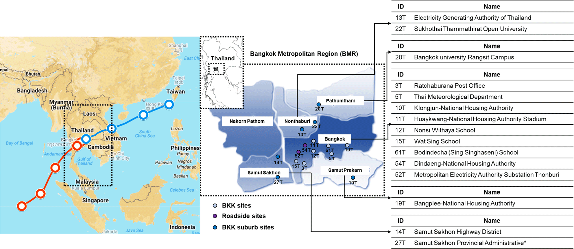
Figure 1 Map of BMR, the location of monitoring stations and two major monsoons winds (from NOAA HYSPLIT back trajectory model). Three monitoring station types (BKK sites, roadside sites and BKK suburb sites) are shown as light blue dots, purple dots and blue dots, respectively. (Note: * the station has been closed since 1 October 2013.)

2 Methodology

2.1 Study area

Figure 1 shows a map of BMR, the location of monitoring stations in this study and major monsoon winds over this region. BMR refers to BKK and the five adjacent provinces, i.e., Nakhon Pathom, Pathum Thani, Nonthaburi, Samut Prakan and Samut Sakhon. These provinces are linked to BKK in terms of traffic and industrial development (Zhang and Oanh, 2002). Thailand has three official seasons – local summer (February to May), rainy seasons (May to October) and local winter (October to February) as per the Thai Meteorological Department (TMD) (TMD, 2015). During the rainy season, this region's weather is influenced by southwest monsoon wind that travels from the Indian Ocean to Thailand. This marine air mass contains a large amount of moisture, resulting in the wet season in Thailand. During this season, Thailand is characterized by cloudy weather with high precipitation and high humidity. From October to April, this region is influenced by northeast monsoon wind that travels from the northeastern and the northern parts of Asia (China and Mongolia). This monsoon wind brings a cold and dry air mass, which leads to the dry season (local summer and local winter) in Thailand. The local winter in Thailand is characterized by cool and dry weather, while the local summer is characterized by hot (35 to 40^∘) to extremely hot weather (> 40^∘) due to strong solar radiation. During the dry season, storms may occur during the seasonal transition (TMD, 2015).

Transportation and industrial sectors are considered to be the major sources of air pollutants in the study area (Watcharavitoon et al., 2013). In 2014, ∼36 million new vehicles were registered in Thailand, and 29 % of these cars were registered in BKK (DLT, 2015). About 56 % and 28 % of the registered vehicles in BKK were gasoline and diesel engines, respectively. The remaining 16 % were run on compressed natural gas (CNG) (DLT, 2017). There are a variety of metal, auto parts, paper, plastic, food and chemical manufacturing facilities and power plants in the outskirts of BKK (DIW, 2016a, b, c, d, e).

2.2 Data collection and data analysis

Over the 5-year period (1 January 2010 to 31 December 2014), hourly observations from 15 Pollution Control Department (PCD) monitoring stations were analyzed. The monitoring stations are assigned to three categories: BKK sites, roadside sites and BKK suburb sites. BKK sites refer to the monitoring stations that are located within BKK's residential, commercial, industrial and mixed areas. They are within ∼50 to 100 m of the road. Roadside sites refer to the monitoring stations that are located in BKK within 2 to 5 m of the road (Zhang and Oanh, 2002). BKK suburb sites refer to the monitoring stations that are located in the provinces adjacent to BKK (Fig. 1). Quality assurance and quality control on the data set were performed by PCD prior to receiving the data. Hourly observations of the gaseous pollutants and meteorological parameters were automatically collected with autocalibration at the monitoring stations. Manual quality control was performed when unusual observations were found. An external audit of the equipment and monitoring stations was done every year. The data availability and details of equipment calibrations are provided in Fig. S1, Sect. S1, Supplement.

Gaseous species were measured at 3 m above ground level (a.g.l.). CO was measured using nondispersive infrared detection (Thermo Scientific 48i). NO and NO₂ were measured using chemiluminescence detection (Thermo Scientific 42i). SO₂ was measured using ultraviolet (UV) fluorescence detection (Thermo Scientific 43i), and O₃ is measured by using UV absorption photometry detection (Thermo Scientific 49i). The meteorological parameters including wind speed (WS) and wind direction (WD) were measured at 10 m a.g.l. by a cup anemometer and potentiometer wind vanes. Temperature (T) and relative humidity (RH) were measured at 2 m a.g.l. by a thermistor and thin film capacitor, respectively (Watchravitoon et al., 2013). All the meteorological measurements were made by Met One or an equivalent method.

Data analysis, statistical analysis and plots were developed using Excel 2016. Predominant wind directions related to O₃ concentrations are obtained using the Openair package (tool for the analysis of air pollution data) on the RStudio program (https://www.rstudio.com/, last access: 6 February 2018).

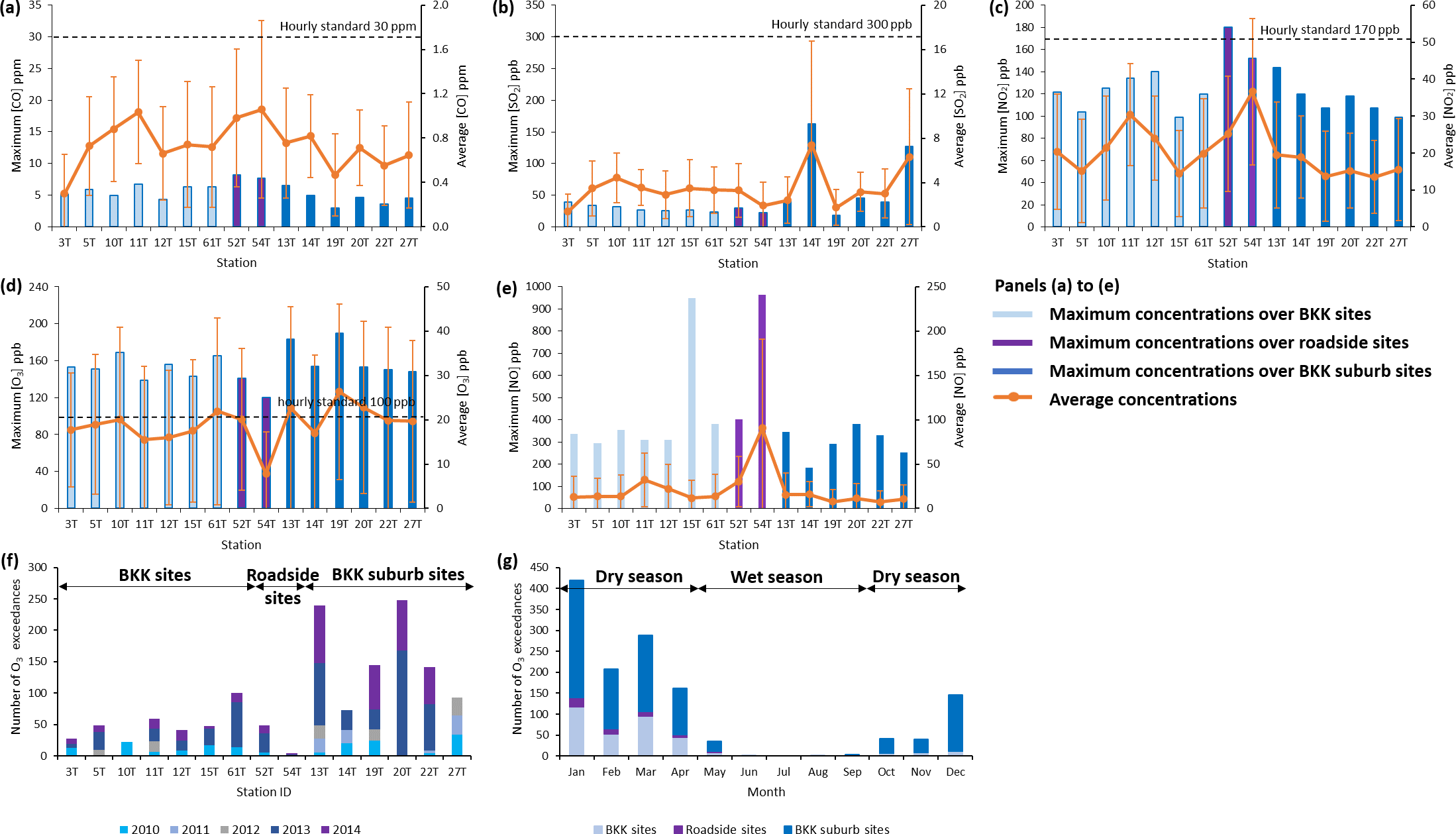
Figure 2 Maximum (vertical bars) and average (solid line) concentrations of (a) CO, (b) SO₂, (c) NO₂ (d) O₃ and (e) NO from the 15 monitoring stations, from 2010 to 2014, are compared with the hourly NAAQs (dotted line) of Thailand (except NO, which is not a criteria pollutant). The number of hourly O₃ exceedances is shown by (f) locations and (g) seasons.

Figure 3 Diurnal variations in gaseous species. The plots provide the average concentrations of O₃, NO and NO₂ in ppb, the average concentrations of CO in ppm, and the average concentrations of SO₂ in ppb at (a) BKK sites, (b) roadside sites and (c) BKK suburb sites. Vertical bars provide ±1 standard deviation of the species concentrations.

3 Result and discussion

3.1 Status of pollution in BMR from 2010 to 2014

Figure 2a to e show the maximum and average concentrations of gaseous pollutants, from 2010 to 2014 from the 15 monitoring stations. These concentrations are compared with the hourly NAAQs of Thailand (NAAQs of Thailand for hourly CO, NO₂, SO₂ and O₃ are 30 ppm, 170 ppb, 300 ppb and 100 ppb, respectively (PCD, 2018)). Since NO is not a criteria pollutant, only the maximum and average concentrations are presented. During the study period, the maximum concentrations of CO, NO₂ and SO₂ were mostly at their hourly standards (an exceedance of NO₂ was found at monitoring station 52T during 2013). However, the maximum concentrations of O₃ exceeded its standard. Elevated CO, NO and NO₂ concentrations were observed more frequently at roadside sites than other sites. The average concentrations of CO, NO and NO₂ at roadside sites were $\sim \mathrm{1.0}\pm \mathrm{0.1}$ ppm, $\sim \mathrm{60.5}\pm \mathrm{42.7}$ ppb, and $\sim \mathrm{30.9}\pm \mathrm{8.1}$ ppb, respectively. Elevated SO₂ was more commonly observed at BKK suburb sites than other sites. The average concentrations of SO₂ at BKK suburb sites were $\sim \mathrm{4.0}\pm \mathrm{2.3}$ ppb. The average concentrations of O₃ during the daytime (06:00 to 18:00 LT) over BKK sites, roadside sites and BKK suburb sites were $\sim \mathrm{24.4}\pm \mathrm{13.5}$, $\sim \mathrm{18.2}\pm \mathrm{12.3}$ and $\sim \mathrm{27.7}\pm \mathrm{14.7}$ ppb, and their values during the nighttime (18:00 to 6:00 LT) were $\sim \mathrm{11.3}\pm \mathrm{3.3}$, $\sim \mathrm{9.1}\pm \mathrm{4.9}$ and $\sim \mathrm{14.2}\pm \mathrm{5.4}$ ppb, respectively. The 24 h average O₃ concentrations were highest at BKK suburb sites ($\sim \mathrm{21.4}\pm \mathrm{3.3}$ ppb), followed by BKK sites (18.6±2.3 ppb) and roadside sites (13.9±8.6 ppb). Statistical analyses of the concentrations of gaseous pollutants from the three monitoring station types are provided in Table S1, Sect. B, Supplement.

The seasonal variations in the gaseous pollutants reveal that, in general, elevated concentrations were observed during dry seasons and they decreased during wet seasons (Fig. S2, Sect. S3). Interannual variations in the gaseous pollutants reveal that while the concentrations of CO, NO₂ and SO₂ decreased or remained constant, the concentration of O₃ tended to increase during the study period (Fig. S3, Sect. S4).

An O₃ exceedance was recorded when an hourly concentration of O₃ was greater than 100 ppb (hourly O₃ standard). Figure 2f and g illustrate the number of hourly O₃ exceedances, which are shown by location and by seasons. The hourly O₃ exceedances at BKK suburb sites were more frequently observed than at the other sites. The average number of hourly O₃ exceedances was ∼16 h yr⁻¹ at BKK sites, ∼9 h yr⁻¹ at roadside sites and ∼43 h yr⁻¹ at BKK suburb sites. The hourly O₃ exceedances were commonly observed during the dry season, less so during the transitional period between the seasons (May) and rarely during the wet season.

3.2 Diurnal variation in the gaseous species

Diurnal variations in gaseous pollutant are shown in Fig. 3a to c. The diurnal variations in O₃ show a single-peak pattern (Aneja et al., 2001) with the concentrations increasing after sunrise and reaching the peak ∼ 15:00 local time (LT). The concentrations begin to decline in the evening and reach the minimum concentrations ∼ 07:00 LT the next morning. The concentrations of O₃ at the peaks were ∼40 ppb at BKK sites, ∼30 ppb at roadside sites and ∼45 ppb at BKK suburb sites. The diurnal variations in NO show a bimodal pattern with the concentrations reaching the first and the second peak ∼ 07:00 to 09:00 and ∼ 21:00 to 22:00 LT, respectively. The concentrations of NO at the first and the second peak were ∼40 and ∼23 ppb at BKK sites, ∼110 and ∼73 ppb at roadside sites, and ∼30 and ∼13 ppb at BKK suburb sites. The concentrations of NO₂ at the first and the second peak were ∼23 and ∼28 ppb at BKK sites, ∼33 and ∼37 ppb at roadside sites, and ∼20 and ∼22 ppb at BKK suburb sites. Even the diurnal variations in NO_x show a bimodal pattern; at roadside sites the pattern was flatter than at other sites. The flatter pattern of NO_x at roadside sites reveals that this monitoring station type was affected by a high concentration of NO_x all day. The diurnal variations in CO show a bimodal pattern with the first and the second peak occurring ∼ 08:00 and 21:00 LT, respectively. The concentrations of CO at the first and the second peak were ∼1 ppm (both peaks) at BKK sites, ∼2 and ∼1.5 ppm at roadside sites, and ∼1 ppm (both peaks) at BKK suburb sites. The first peak of the diurnal variations in NO, NO₂ and CO corresponds with the morning rush hour in BKK (07:00 to 09:00 LT). The second peak occurred ∼3 to 5 h after the evening traffic rush hour (16:00 to 18:00 LT) (Leong et al., 2002), due to a combination of pollutant emissions and the collapse of the planetary boundary layer (weak turbulence and diffusion) during this time. The diurnal variations in SO₂ show a bimodal pattern with the first and the second peak of SO₂ occurring ∼ 08:00 and 21:00 LT, respectively. The concentrations of SO₂ at the first and the second peak were ∼4 and ∼3 ppb at BKK sites and roadside sites and ∼6 and ∼3 ppb at BKK suburb sites. At the roadside sites, the peaks are more obvious than at the other sites. The result indicates that at this monitoring station type, SO₂ is primarily influenced by emissions from vehicle exhaust using a high sulfur content fuel (Henschel et al., 2013). It is noteworthy that BKK has a large diesel engine fleet (an estimated 25 % of registered vehicles) (DLT, 2015). Diesel fuel contains ∼0.035 % wt sulfur (DOEB, 2017). The season-wise distributions of the diurnal variations are provided in Fig. S4, Sect. S5.

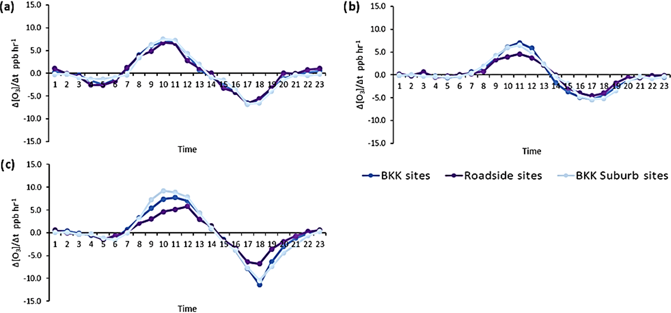
Figure 4 Diurnal variations in the rate of change in O₃ concentration (Δ[O₃]/dt) during (a) local summers, (b) wet seasons and (c) local winters.

Figure 4a to c shows diurnal variations in the rate of change in O₃ concentration (Δ[O₃]/dt) during dry seasons (local summer and local winter) and wet seasons at the three monitoring station types (the data have been averaged for each monitoring station type to capture the rate of change in O₃ concentration characteristics). The diurnal variations in Δ[O₃]/dt are a combination of O₃ chemistry and meteorology. In general, Δ[O₃]/dt during the wet season were lower than those during dry season. However, during local winter, the rates of change in O₃ concentration were the highest. The Δ[O₃]/dt at the three monitoring station types, from 10:00 to 11:00 LT, were 4.5 to 7.0 ppb h⁻¹ during wet seasons, 6.7 to 7.5 ppb h⁻¹ during local summers and 5.7 to 9.2 ppb h⁻¹ during local winters. The Δ[O₃]/dt became negative from 14:00 to 15:00 LT. As expected, the rate of change in O₃ concentration was nearly constant during the nighttime. Rapid changes in the mixing height and solar insolation during the morning increases Δ[O₃]/dt. After sunset, the formation of O₃ is inhibited and the planetary boundary layer becomes more stable resulting in O₃ reduction through chemical reactions (for example, the oxidation of O₃ by NO_x) and physical processes (for example, dry deposition to the earth surface) (Naja and Lal, 2002).

3.3 Photochemical reaction and interconversion between O₃, NO and NO₂

The primary precursors for tropospheric O₃, in the urban environment, are NO_x and non-methane volatile organic compounds (VOCs), methane or CO (The Royal Society, 2008; Monks et al., 2009; Cooper et al., 2014). While NO_x was measured continuously at all the monitoring sites, VOCs were measured periodically only at one monitoring station, limiting its usefulness as part of this study. In this study, the photostationary state (PSS) is applied through the chemical reactions of O₃ formation from 10:00 to 16:00 LT. This time window is chosen due to the fully developed planetary boundary layer with well-mixed condition (Pochanart et al., 2001) to avoid the accumulation of air pollutants by surface inversion. Analysis and calculation are performed only during the dry season to eliminate the effects of the removal process by wet deposition.

The relationship among NO, NO₂ and O₃ under PSS is presented by Eq. (1) (Seinfeld and Pandis, 1998).

$$\begin{array}{}\text{(1)}& {\displaystyle }[{\mathrm{O}}_{\mathrm{3}}{]}_{\mathrm{PSS}}={\displaystyle \frac{j_{\mathrm{1}}\left[{\mathrm{NO}}_{\mathrm{2}}\right]}{k_{\mathrm{3}}\left[\mathrm{NO}\right]}},\end{array}$$

where [O₃]_PSS is the concentration of O₃ at PSS and j₁ and k₃ are the reaction rate coefficient of the photochemical reaction of NO₂ and the reaction rate coefficient of the chemical reaction between NO and O₃, respectively.

The values for k₃ (ppm⁻¹ min⁻¹) are calculated by Eq. (2) (Seinfeld and Pandis, 1998; Tiwari et al., 2015).

$$\begin{array}{}\text{(2)}& {\displaystyle }{k}_{\mathrm{3}}=\mathrm{3.23}\times {\mathrm{10}}^{\mathrm{3}}\exp [-\mathrm{1430}/T]\end{array}$$

During dry seasons, the values of j₁ ranged from 0.12 to 1.22 min⁻¹, and the average of those at BKK sites, roadside sites and BKK suburb sites were 0.74±0.2, 0.64±0.3 and 0.55±0.3 min⁻¹, respectively. The rate coefficients are calculated using the NCAR TUV model for 10:00 to 16:00 LT during the 2010 dry season at the latitude and longitude of 13.76^∘ N and 100.50^∘ E. The average j₁ value calculated from the NCAR TUV model is 0.021±0.0024 s⁻¹, which is similar to the calculated j₁ values from Eq. (1) (j₁ ranges from 0.008 to 0.013 s⁻¹). The values of j₁ from this study are similar to those values at an urban background site in Delhi, India (values of j₁ ranged from 0.4 to 1.8 min⁻¹ and the average was 0.8 min⁻¹) (Tiwari et al., 2015) and those values collected during daytime in November in the UK (value of j₁ was ∼0.14 min⁻¹) (Clapp and Jenkin, 2001).

The values of k₃, during dry seasons, ranged from 28.3 to 30.9 ppm⁻¹ min⁻¹, and the average of those at BKK sites, roadside sites and BKK suburb sites were 29.8±0.7, 29.7 and 29.8±0.7 ppm⁻¹ min⁻¹, respectively. The ratio of [NO₂] and [NO] was ∼1.9. The statistical analysis of j₁ (min⁻¹ and s⁻¹) and k₃ (ppm⁻¹ min⁻¹ and cm³ molecule⁻¹ s⁻¹) at the three monitoring station types using Eq. (1) and the average j₁ calculated from the NCAR TUV model are provided in Table S2, Sect. F.

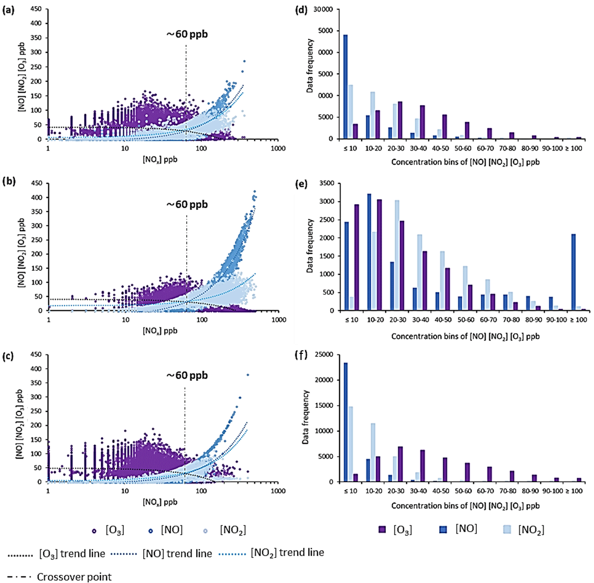
Figure 5 Relationships and crossover points of NO, NO₂ and O₃ at (a) BKK sites, (b) roadside sites and (c) BKK suburb sites and concentration distributions of those species at (d) BKK sites, (e) roadside sites and (f) BKK suburb sites.

Figure 5a to c shows the relationships between NO, NO₂ and O₃, their crossover points, and concentration distributions. The crossover point among species occurs when the concentration of NO_x is ∼60 ppb. At this point, two regimes are identified, including a low-NO_x regime and a high-NO_x regime. Under the low-NO_x regime ([NO_x] < 60 ppb), O₃ is the dominant species and NO₂ concentrations are higher than NO for NO_x species. Conversely, under the high-NO_x regime ([NO_x]> 60 ppb), NO and NO₂ increase and the concentrations of O₃ rapidly decrease. Under the high-NO_x regime, the decline in O₃ trend lines may describe the O₃ removal process through the titration of O₃ by NO.

3.4 Local and regional contribution to O_x

The O_x concentration is the summation of O₃ and NO₂ concentration. Under the PSS condition, the concentration of NO, NO₂ and O₃ approaches an equilibrium and the concentration of O_x may be considered constant (Keuken et al., 2009). Since the conversion between O₃ and NO₂ in the urban and suburban atmosphere is rapid, the use of O_x to represent the production of oxidants is more appropriate than only using O₃ (Lu et al, 2010). The local or NO_x-dependent contribution refers to O_x concentration that are influenced by a concentration of the local pollutants. The regional or NO_x-independent contribution refers to the background concentration of O_x that is not influenced by changes in the local pollutants (Clapp and Jenkin, 2001; Tiwari et al., 2015).

Table 1 The comparison of fitted linear regression lines from this study, including at BKK sites, roadside sites and BKK suburb sites with fitted linear regression lines from other studies.

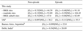
^a Clapp and Jenkin (2001). ^b Mazzeo et al. (2005). ^c Tiwari et al. (2015).

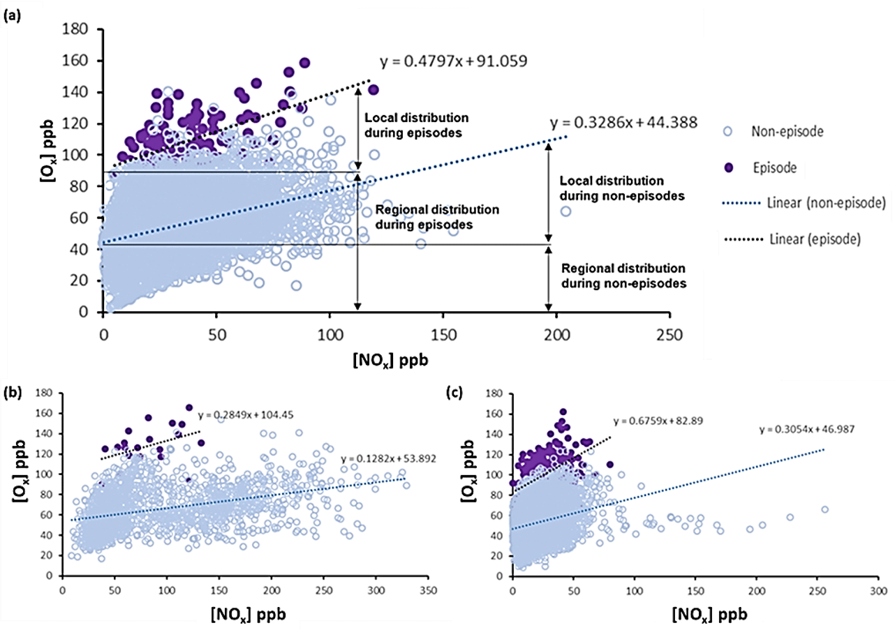
Figure 6 The effects of local and regional contributions on O_x during non-episode and episode days at (a) BKK sites, (b) roadside sites and (c) BKK suburb sites.

Figure 6a to c show the local and regional contributions of O_x at the three monitoring station types. The effects of the local and regional contributions to O_x concentration are analyzed by plotting O_x concentrations against NO_x concentrations and fitting the plot with a linear regression ($y=mx+c$). The concentrations of NO_x and O_x are referred to as x and y, respectively. The slope of the linear regression (m) implies the local contribution, and the intercept with the y axis (c) implies the regional (background) contribution (Aneja et al., 2000; Clapp and Jerkin, 2001; Notario et al., 2012). Table 1 shows the comparison between fitted linear regressions from this study and fitted linear regression lines from other studies. The average background O_x concentrations over BMR during non-episodes ([O₃]_hourly < 100 ppb) and episodes ([O₃]_hourly > 100 ppb) were ∼48 and ∼95 ppb, respectively. The local and regional contributions during the episode days, in general, were about double of those during the non-episode days. The results reveal that elevated O₃ concentrations during the episode days are influenced by both the local and regional contributions of O_x. It is noteworthy that the pattern of the local and regional contributions at roadside sites during non-episode periods is composed of two NO_x concentration regimes. The low-NO_x regime (NO_x < 60 ppb) resembles the local and regional contributions during non-episodes over BKK suburb sites. The high-NO_x regime (NO_x > 60 ppb) may represent the typical characteristics of air quality near roads.

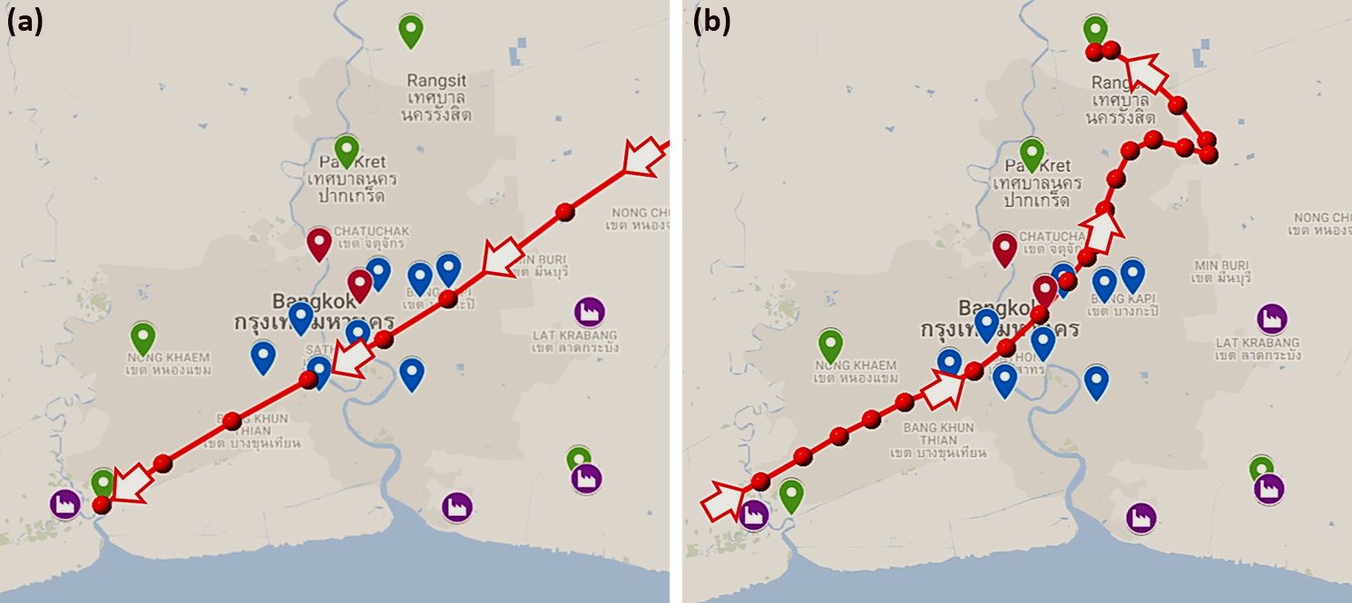
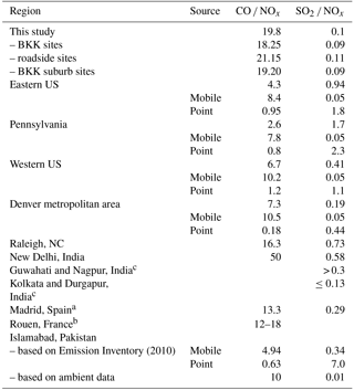
Figure 7 Backward trajectories from the HYSPLIT model reveal a (a) NE wind direction (13 January 2010) and (b) SW wind direction (1 January 2010).

The local contributions from the fitted linear regressions are compared with the local contribution that is calculated from the delta O₃ method. A delta O₃ (ΔO₃) analysis was performed to reflect on the intensity of O₃ production in the BMR area (Lindsay and Chameides, 1988). Lindsay et al. (1989) analyzed high-O₃ events in Atlanta, GA, USA, and showed that rural background O₃ during high O₃ concentrations ([O₃] > 80 ppb) in the Atlanta metropolitan area was higher than its average and the concentration of O₃ increased from ∼15 to 20 ppb when the air mass traveled across the city. This enhanced the total O₃ concentration from 80 to 85 ppb. In our study, the differences in the concentrations of O₃ at the upwind and downwind monitoring stations (monitoring stations 20T and 27T) are averaged. The conditions to calculate ΔO₃ in this study are as follows (1) high O₃ concentrations ([O₃] > 80 ppb) were observed at at least one of the two monitoring stations; (2) the calculation is performed from 10:00 to 16:00 LT during the dry season to avoid the accumulation of air pollutants by surface inversion and the effects of the removal process by wet deposition; (3) National Oceanic and Atmospheric Administration (NOAA) HYSPLIT model backward trajectories revealed N–NE, S–SW wind directions (Fig. 7). Even the O₃ concentrations at the downwind monitoring stations are expected to be greater than the O₃ concentrations at the upwind monitoring stations, a negative ΔO₃ may be found. The negative ΔO₃ suggests the deposition of O₃ and/or that O₃ was consumed as it passes over the city and/or that there may have been a wind reversal so that air already polluted by the metropolitan area was brought back in to the city (Lindsay et al., 1989). The ΔO₃ in BMR ranged from −53 to 86 ppb (average ∼10.4 ppb) and ranged from −66 to 96 ppb (average ∼9.4 ppb) when the predominant wind directions advecting into the city were from NE and SW, respectively. Thus, we find that there was a ∼10 ppb enhancement of the O₃ concentration during the air pollution high O₃ concentration in BMR ([O₃] > 80 ppb), which corroborates local O₃ production analysis based on linear regression.

3.5 Correlation of air pollutants

3.5.1 Local sources analysis

The characteristics of emission sources are often determined by the ratios between CO and NO_x (CO ∕ NO_x) and SO₂ and NO_x (SO₂ ∕ NO_x). In general, the major sources of NO_x are point sources and mobile sources. However, NO_x from point sources is more likely correlated with SO₂. NO_x from mobile sources is more likely correlated with CO (Parrish et al., 1991). Therefore, the characteristics of mobile sources are high CO ∕ NO_x ratios and low SO₂ ∕ NO_x ratios. In contrast to mobile sources, the characteristics of point sources are low CO ∕ NO_x ratios and high SO₂ ∕ NO_x ratios (Parrish et al., 1991; Rasheed et al., 2014).

Table 2 The comparison of CO ∕ NO_x and SO₂ ∕ NO_x ratios from this study with other studies (modified from Rasheed et al., 2014).

^a Fernandez-Jiménez et al. (2003). ^b Coppalle et al. (2001). ^c Mallik and Lal (2014).

Table 2 shows the comparison between the CO ∕ NO_x and SO₂ ∕ NO_x ratios from this study when compared with other studies. The ratio of CO ∕ NO_x is 19.8, and the ratio of SO₂ ∕ NO_x is 0.1 over BMR. This suggests that the major contributors of primary pollutants over the BMR are mobile sources. However, this region may be influenced by manufacturing facilities' point sources (SO₂ contributor) on the outskirts of the BKK. These point sources will impact the concentrations of SO₂, NO_x and CO. Correlations among species are provided in Table S3, Sect. G.

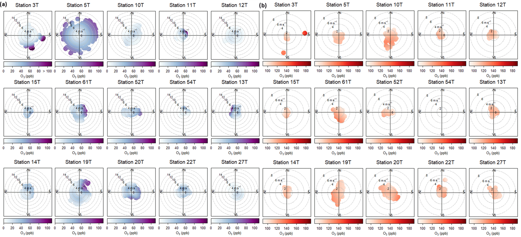
Figure 8 Relationship between the concentrations of O₃, wind speeds and wind directions during (a) O₃ episodes ([O₃]_hourly > 100 ppb) and (b) during non-O₃-episodes ([O₃]_hourly≤100 ppb) over BMR from 2010 to 2014.

3.5.2 Effects of pollutant transport

In general, O₃ has a short lifetime in the polluted urban atmosphere (approximately hours). However, O₃ has a longer lifetime of several weeks in the free troposphere. This occurrence may allow O₃ to be transported over continental scales (Stevenson et al., 2006: CO ∕ NO_x; Young et al., 2013: CO ∕ NO_x; Monks et al., 2015). Figure 8 shows O₃ concentrations, during episodes and non-episodes, with predominant wind directions and wind speeds. The results show that O₃ exceedances are associated with low wind speed and predominant wind directions, i.e., the origins of the air masses. In general, elevated O₃ concentrations were observed with a wind speed lower than 4 ms⁻¹ with northerly winds (station 22T), southerly winds (stations 3T, 10T, 19T, 20T and 61T) and westerly winds (station 52T). It is noteworthy that the southerly winds, generally, bring cleaner marine air mass to the land. However, under a stagnant condition (i.e., low wind speed), elevated O₃ concentrations were observed during southerly winds (Sahu et al., 2013a, b).

Table 3 Number of hours for the different AQI categories of O₃ over the BMR from 2010 to 2014.

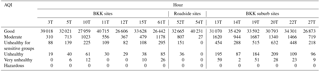
3.6 Air quality index for O₃ management

In the US, the AQI for air pollutants is divided into six categories (good, moderate, unhealthy for sensitive groups, unhealthy, very unhealthy and hazardous). These categories are nonlinear and relate to human health (U.S. EPA, 2017a, b, c). In Thailand, the NAAQs for the air pollutant species are pegged at an AQI value of 100. In this study, the severity of O₃ concentrations in BMR is evaluated by AQI for O₃. Table 3 provides the ambient air quality over BMR from 2010 to 2014 based on the AQI of O₃. Based on the AQI for O₃, during the study period, the majority of air quality over BMR was in the good AQI category (∼97 %) followed by the moderate air quality category (∼2.3 %). However, the unhealthy for sensitive groups (∼0.7 %), unhealthy (∼0.3 %) and very unhealthy (∼0.04 %) O₃ air quality categories were observed. Generally, BKK suburb sites have a higher number of hours that were categorized as unhealthy for sensitive groups, unhealthy and very unhealthy than BKK and roadside sites. The average number of hours that were categorized as unhealthy for sensitive groups, unhealthy and very unhealthy over BKK suburb sites were 425.8, 146.7 and 28.7 h. The calculation of the AQI for O₃ can be found in Figs. S5 and S6, Sect. S8.

This study provides measurements and analysis for the gaseous criteria pollutants. However, in order to provide a well-established air quality management policy, the integration of multidisciplinary analysis is needed. This will include scientific, socioeconomic and policy analysis (Aneja et al, 2001). The results from this study revealed evidence of O₃ air quality standards being breached. This resulted in adverse health effects, human welfare, economics, and environment over BMR. Ratio analysis suggests that the first priority should be controlling pollution emissions from local sources that are primarily mobile. The complex relationship between O₃ and its precursors and the effects of pollution transport show that decreasing only NO_x emissions and/or local emissions may not be an effective policy to reduce O₃ because of regional air pollution transport (i.e., ozone and its precursors contribute to O₃ exceedances). To identify the proportional contribution between local and regional sources of O₃ concentrations during selected O₃ episode days, atmospheric modeling is needed to quantify various processes that contribute to the ambient concentration at specific locations. This scientific analysis provides a framework for the process of establishing an air quality policy while analyzing socioeconomic impacts.

4 Conclusions

Among measured gaseous criteria pollutants, O₃ is the only species whose concentrations frequently exceed the NAAQs of Thailand. The O₃ exceedances occur during the dry season (local summer and local winter) and more frequently occur over BKK sites and BKK suburb sites than roadside sites. On average, the number of hourly O₃ exceedances at BKK sites, roadside sites and BKK suburb sites was ∼16, ∼9 and ∼43 h yr⁻¹, respectively. The lower number of O₃ exceedances at roadside sites demonstrates the effects of the titration of O₃ by NO due to high concentrations of NO that were generally observed at this monitoring station type (average [NO]${}_{\mathrm{hourly}}=\sim \mathrm{166.0}\pm \mathrm{19.8}$ ppb). Under the photostationary state assumption, during the dry season, the values of the reaction rate coefficient of the photochemical reaction of NO₂ (j₁) and the reaction rate coefficient of the chemical reaction between NO and O₃ (k₃) from 0.12 to 1.22 min⁻¹ and range from 28.3 to 30.9 ppm⁻¹ min⁻¹, respectively. NO_x values of ∼60 ppb mark the threshold for the interconversion between O₃, NO and NO₂. Under the low-NO_x regime ([NO_x] < 60 ppb), O₃ is the dominant species. On the other hand, under the high-NO_x regime ([NO_x] > 60 ppb), the concentrations of O₃ rapidly decrease. The decrease in O₃ under the high-NO_x regime describes the important role of NO in destroying O₃ in the atmosphere in polluted environments. The local and regional contributions of O_x concentrations under stagnant conditions (wind speed < 4 m s⁻¹) and the origin of air masses containing O₃ and its precursors are associated with elevated O₃ concentrations in this area. During O₃ episodes, the values of the local and regional contributions were about double those during non-episodes. The air quality index for O₃ reveals evidence of air quality standards being breached in BMR, resulting in potentially adverse health effects. To achieve O₃ reduction, control strategies may be needed. Emissions from mobile sources may be the first priority to manage O₃, since BMR is more likely to be affected by mobile sources than point sources (CO ∕ NO_x =19.8 and SO₂ ∕ NO_x =0.1). Due to the highly nonlinear physical and chemical processes governing the atmosphere, control strategies need to be evaluated in a more comprehensive approach. Air quality modeling of pollution episodes in the BMR would be an appropriate approach to accurately quantify various atmospheric processes contributing to high O₃ concentrations in BMR.