the Creative Commons Attribution 4.0 License.
the Creative Commons Attribution 4.0 License.
 | 30 Aug 2018
Retrieval of desert dust and carbonaceous aerosol emissions over Africa from POLDER/PARASOL products generated by the GRASP algorithm
Daven K. Henze
Tatyana Lapyonak
Mian Chin
Fabrice Ducos
Pavel Litvinov
Xin Huang
Lei Li
Understanding the role atmospheric aerosols play in the Earth–atmosphere system is limited by uncertainties in the knowledge of their distribution, composition and sources. In this paper, we use the GEOS-Chem based inverse modelling framework for retrieving desert dust (DD), black carbon (BC) and organic carbon (OC) aerosol emissions simultaneously. Aerosol optical depth (AOD) and aerosol absorption optical depth (AAOD) retrieved from the multi-angular and polarimetric POLDER/PARASOL measurements generated by the GRASP algorithm (hereafter PARASOL/GRASP) have been assimilated. First, the inversion framework is validated in a series of numerical tests conducted with synthetic PARASOL-like data. These tests show that the framework allows for retrieval of the distribution and strength of aerosol emissions. The uncertainty of retrieved daily emissions in error free conditions is below 25.8 % for DD, 5.9 % for BC and 26.9 % for OC. In addition, the BC emission retrieval is sensitive to BC refractive index, which could produce an additional factor of 1.8 differences for total BC emissions. The approach is then applied to 1 year (December 2007 to November 2008) of data over the African and Arabian Peninsula region using PARASOL/GRASP spectral AOD and AAOD at six wavelengths (443, 490, 565, 670, 865 and 1020 nm). Analysis of the resulting retrieved emissions indicates 1.8 times overestimation of the prior DD online mobilization and entrainment model. For total BC and OC, the retrieved emissions show a significant increase of 209.9 %–271.8 % in comparison to the prior carbonaceous aerosol emissions. The model posterior simulation with retrieved emissions shows good agreement with both the AOD and AAOD PARASOL/GRASP products used in the inversion. The fidelity of the results is evaluated by comparison of posterior simulations with measurements from AERONET that are completely independent measurements and more temporally frequent than PARASOL observations. To further test the robustness of our posterior emissions constrained using PARASOL/GRASP, the posterior emissions are implemented in the GEOS-5/GOCART model and the consistency of simulated AOD and AAOD with other independent measurements (MODIS and OMI) demonstrates promise in applying this database for modelling studies.
- Article
(12660 KB) - Full-text XML
- BibTeX
- EndNote


Atmospheric aerosols have a variety of sources and complex chemical compositions. Desert dust (DD) aerosol is one of the most abundant types of aerosol by mass, while the range of global dust emission estimates spans a factor of about 5 (Huneeus et al., 2011). Primary carbonaceous aerosol, which consists of black carbon (BC) and organic carbon (OC) from combustion of fossil fuels, biofuels and biomass, has strong light absorption that can affect the energy balance of the Earth–atmosphere system (Bond et al., 2013). High uncertainty in carbonaceous aerosol emissions (e.g., Bond et al., 2004) translates into a significantly high uncertainty in evaluating their climate effects (Textor et al., 2006). The Intergovernmental Panel on Climate Change (IPCC) estimates the global mean direct shortwave radiative forcing due to primary carbonaceous aerosol to be −0.1 W m−2 in their 2001 report, in 2007 they raise it to 0.18 W m−2 and in the latest report (IPCC, 2013) the value comes to 0.31 W m−2 (Myhre et al., 2013). Furthermore, desert dust and carbonaceous aerosols can have deleterious impacts on regional air quality and public health (Chin et al., 2007; Monks et al., 2009; Li et al., 2013). Thus, observations are needed to accurately evaluate their emissions in order to better understand the role that atmospheric aerosols play in the Earth–atmosphere system (Bellouin et al., 2005).
Space-borne remote-sensing instruments offer an integrated atmospheric column measurement of the amount of light scattering by aerosols through modification of diffuse and direct solar radiation. Numerous satellite observations of the spatial and temporal distribution of aerosols have been conducted in the last 2 decades (King et al., 1999; Kaufman et al., 2002; Lenoble et al., 2013). The satellite retrievals of aerosol optical depth (AOD) and aerosol absorption optical depth (AAOD) are directly related to light extinction and absorption due to the presence of aerosol particles. AOD is a basic optical property derived from many Earth-observation satellite sensors, such as AVHRR (Advanced Very High Resolution Radiometer), MODIS (Moderate Resolution Imaging Spectroradiometer), MISR (Multi-angle Imaging SpectroRadiometer) and POLDER (Polarization and Directionality of the Earth's Reflectances) (Goloub et al., 1999; Geogdzhayev et al., 2002; Kahn et al., 2009; Tanré et al., 2011; Levy et al., 2013). AAOD is another valuable product to quantify the solar absorption potential of aerosols; however, only a few satellite aerosol products can provide retrievals of AAOD, and only with limited accuracy, for example OMI (Ozone Monitoring Instrument) on the Aura satellite making measurements in the UV range that have sensitivity to aerosol absorption (Torres et al., 2007; Veihelmann et al., 2007).
Despite their ability to provide global coverage in high spatial resolution, satellite measurements alone are not sufficient for addressing the question regarding the distributions, magnitudes and fates of aerosols in the atmosphere. These aspects can be studied using chemical transport models (CTMs), which rely on meteorological data from external databases with atmospheric physics, considering the physical and chemical processes in the atmosphere, and allow modelling of the detailed distribution of aerosol for any chosen time period (e.g. models by Balkanski et al., 1993; Chin et al., 2000; Takemura et al., 2000; Ginoux et al., 2001; Bessagnet et al., 2004; Grell et al., 2005; Spracklen et al., 2005; Mann et al., 2010). However, CTM simulations are limited by uncertainties in knowledge of aerosol emission characteristics, knowledge of atmospheric and aerosol processes, and the meteorological data used. As a result, even the most recent models are expected to capture only the principal global features of aerosol. For example, among different models, quantitative estimates of average regional aerosol properties often disagree by amounts exceeding the uncertainty of remote sensing of aerosol observations (Chin et al., 2002, 2014; Kinne et al., 2003, 2006; Textor et al., 2006). Therefore, there are diverse and continuing efforts to harmonize and improve aerosol modelling by refining the meteorology, atmospheric process representations, emissions and other components (e.g. aerosol aging scheme, particle mixing state) (Watson et al., 2002; Dabberdt et al., 2004; Generoso et al., 2007; Ghan and Schwartz, 2007; He et al., 2016; R. Wang et al., 2014, 2016).
One of the most promising approaches for reducing model uncertainty is to improve the aerosol emission fields (that is input for the models) by inverse modelling, i.e. fitting satellite observations and model estimates and by adjusting aerosol emissions (e.g. Bennett, 2002). For example, Dubovik et al. (2008) developed an algorithm for inverting CTMs and implemented the approach to retrieve distributions of aerosol emissions using MODIS data. The algorithm was used to implement the first formal retrieval of global spatial and temporal emission distributions of fine-mode aerosol from the MODIS fine-mode AOD data. Wang et al. (2012) and Xu et al. (2013) use MODIS radiances to constrain aerosol sources over China. Huneeus et al. (2012, 2013) optimize global aerosol emissions using MODIS AOD with a simplified aerosol model (Huneeus et al., 2009). However, as discussed in Dubovik et al. (2008) and Meland et al. (2013), MODIS AOD (as well as currently available aerosol satellite data) contains only limited information to evaluate aerosol types, properties or speciated emissions. Further, inconsistencies among representations of aerosol microphysics between the CTM and the aerosol retrieval algorithm can have significant influences on inverse modelling of aerosol sources (e.g. Drury et al., 2010; Wang et al., 2010). Therefore, the retrieval of aerosol emissions from satellite observations remains very challenging.
Recently a new dataset of spectral AOD and AAOD was generated using the GRASP (General Retrieval of Atmosphere and Surface Properties) algorithm from POLDER/PARASOL (Polarization & Anisotropy of Reflectances for Atmospheric Sciences coupled with Observations from a Lidar) instrument (Dubovik et al., 2011, 2014; data available from ICARE data distribution portal: http://www.icare.univ-lille1.fr/, last access: 8 August 2018). Since several POLDER instruments were launched on different satellites, in the text an abbreviation of PARASOL satellite is used instead of instrument. The PARASOL/GRASP data present new opportunities for constraining DD, BC and OC sources because their optical properties vary dramatically in the spectrum of shortwave visible to near infrared (VIS–NIR) viewed by PARASOL. Polarimetric remote-sensing measurements such as those from PARASOL have been postulated to provide much greater constraints on speciated aerosol emissions and microphysical properties (Meland et al., 2013). DD aerosols are dominated by coarse-mode particles, and their AOD varies slightly in the VIS–NIR spectral range; in contrast, the AOD of fine-mode-dominated BC and OC aerosols decreases sharply in this spectral range. In addition, DD and OC particles absorb more strongly in the UV and shortwave visible channels such as at 443 nm than in the rest of the visible spectrum, while BC particles absorb more ubiquitously (Sato et al., 2003). The GRASP retrieval overcomes the difficulty of deriving aerosol over bright surfaces in the visible wavelengths and GRASP provides both AOD and AAOD even over desert, which should help improve constraints of DD emissions over source regions, rather than having to rely on downwind observations (e.g., Wang et al., 2012).
Here we develop an inverse modelling approach to retrieve the spatial and temporal distributions of DD, BC and OC aerosol emissions simultaneously from PARASOL/GRASP spectral AOD and AAOD using the GEOS-Chem model (Bey et al., 2001) and its adjoint (Henze et al., 2007). Section 2 describes the model and data used in this study. The dust and carbonaceous aerosol model in the GEOS-Chem adjoint of Henze et al. (2007) is that of the GOCART (Goddard Chemistry Aerosol Radiation and Transport) model implemented in GEOS-Chem (Fairlie et al., 2007; Park et al., 2003), which is fully conceptually consistent with the aerosol model used in the inversion by Dubovik et al. (2008). The details of inverse modelling and performance evaluation of the inversion framework using numerical tests are presented in Sect. 3. In order to interpret the retrieval results and improve our understanding of aerosol emissions, we retrieve 1 year of daily DD, BC and OC emissions (see Sect. 4). Evaluation of these inversion results using independent AERONET, MODIS and OMI observations, as well as implementation of the posterior emissions in the GEOS-5/GOCART model, is presented in Sect. 5. Conclusions and discussion of the study's merits and limitations are considered in the Sect. 6.
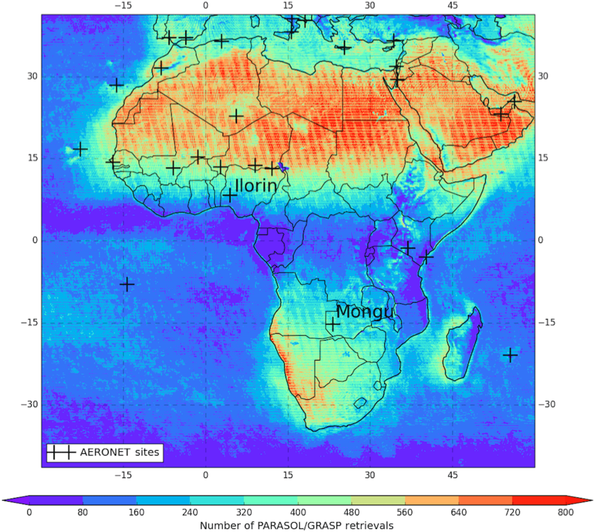
Figure 1Distribution of PARASOL/GRASP AOD retrievals per 0.1∘ × 0.1∘ grid cell over a year (December 2007 to November 2008); the 28 AERONET sites used for validation are also shown with black crosses.
Table 1Aerosol refractive index, size distribution and particle density for DD, BC, OC, SU, SS and host water employed in this study.
2.1 Study area
The study area (30∘ W–60∘ E, 40∘ S–40∘ N) is shown in Fig. 1, which covers all of Africa and the Arabian Peninsula, comprising one of the largest dust source and biomass burning regions of the globe. The spatial and temporal variability in DD, BC and OC aerosols in this area has inspired numerous studies (Duncan et al., 2003; Prospero and Lamb, 2003; Engelstaedter et al., 2006; Liousse et al., 2010; Zhao et al., 2010; Ginoux et al., 2012; Ealo et al., 2016). Figure 1 shows the number of PARASOL/GRASP retrievals per grid box over a year (December 2007 to November 2008) and the 28 AERONET (AErosol RObotic NETwork) (Holben et al., 1998) sites used to evaluate GEOS-Chem model simulations and PARASOL/GRASP retrievals. Note that the GRASP algorithm performs aerosol retrievals at PARASOL's native resolution of 6–7 km; each 0.1∘ grid box could thus have more than one GRASP retrieval, so the number of PARASOL/GRASP retrievals exceeds the number of days in some grid boxes of Fig. 1. The number of GRASP algorithm (see in Sect. 2.3) retrievals over the region of the northern Africa Sahara and the Arabian Peninsula desert is relatively high, whereas other regions have a reduced number of retrievals due to the presence of clouds.
2.2 GEOS-Chem model and its adjoint
GEOS-Chem is a global three-dimensional CTM driven by assimilated meteorological data from the NASA Goddard Earth Observing System Data Assimilation System (GEOS-DAS) (Bey et al., 2001). We use the GEOS-Chem (v9-02) model for aerosol simulation with 47 vertical layers and 2∘ (latitude) × 2.5∘ (longitude) horizontal resolution. DD, BC and OC aerosols are simulated in our study, including seven size bins for resolving dust (Fairle et al., 2007) and the total aerosol mass of BC and OC (Park et al., 2003). Dust simulations in GEOS-Chem (Fairlie et al., 2007) combine the mineral Dust Entrainment and Deposition (DEAD) model (Zender et al., 2003) with the GOCART dust source function (Ginoux et al., 2001). The daily biomass burning sources are calculated from version 3 of the Global Fire Emissions Database (GFED) inventory (van der Werf et al., 2006, 2010; Randerson et al., 2013). The monthly anthropogenic fossil fuel and biofuel BC and OC emissions are adopted from the Bond inventory with the base year 2000 (Bond et al., 2007). The sulfate (SU) and sea salt (SS) aerosol simulation in GEOS-Chem is described in Park et al. (2004) and Jaeglé et al. (2011). The standard aerosol dry deposition in GEOS-Chem is described in Wang et al. (1998) and Wesely (1989) and accounts for gravitational settling and turbulent mixing of particles to the ground layer (Zhang et al., 2001; Pye et al., 2009). Aerosol wet deposition in GEOS-Chem includes wet scavenging in convective updrafts as well as in- and below-cloud scavenging from convective and large-scale precipitation (Liu et al., 2001).
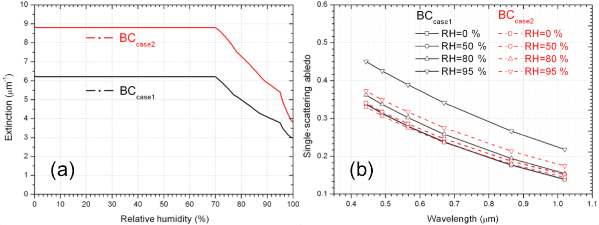
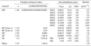
Figure 2(a) The relative humidity dependence of BC particle extinction at 565 nm. (b) Wavelength dependence of BC particle single-scattering albedo at six PARASOL wavelengths.
The GEOS-Chem model assumes external mixing for aerosol components with lognormal size distributions. The modal (rmean) and effective (reff) radius and width (sigm) for each dry aerosol species and their optical properties are specified (see in Table 1). The extinction and scattering coefficients are calculated from size distributions and refractive indices assuming spherical particles. Different aerosol species are considered to have hygroscopic growth rates as a function of ambient relative humidity (RH). The simulated aerosol masses are then converted to AOD (τ) and AAOD (τa) through the general relationship between aerosol optical depth and aerosol mass (Tegen and Lacis, 1996):
where n is the total number of aerosol components, i represents the individual aerosol component, m is aerosol mass, λ is wavelength, ρ is aerosol density, re is particle effective radius, and Qext(λ) and Qabs(λ) are the aerosol extinction and absorption coefficients, respectively. The size distribution and the spectral aerosol refractive index used to calculate Qext(λ) and Qabs(λ) are assumed based on the Global Aerosol Data Set (Koepke et al., 1997), with modifications for dust particles by including a spectral dependence for the imaginary part based on analysis of AERONET measurements (Dubovik et al., 2002b). Further, the particle optical properties Qext(λ) and Qabs(λ) are calculated according to the AERONET kernel based on a mixture of spheroids suggested in studies by Dubovik et al. (2002a, 2006). The particle density and hygroscopic growth rate are described in Chin et al. (2002) and Martin et al. (2003). Table 1 lists the detailed aerosol properties used in this study. Here we consider two cases of BC refractive index. Figure 2a demonstrates the RH dependence of these two cases of BC aerosol extinction (Qext(λ)∕re) at 565 nm, and Fig. 2b presents the wavelength dependence of single-scattering albedo (SSA) for these two cases. The Case 1 BC refractive index is based on Chin et al. (2002) and Martin et al. (2003). More recent studies have recommended a BC refractive index of 1.95–0.79i (Schuster et al., 2005; Bond and Bergstrom, 2006; Koch et al., 2009; Arola et al., 2011), which has a higher absorption and scattering ability than Case 1. Figure 2a shows that the extinctions calculated from the AERONET kernel for Case 2 BC particles are about a factor of 1.5 higher than for Case 1. The difference in SSA is small (Case 2 is about 2 % higher at 565 nm when RH = 0 %); however the difference increases when RH = 95 %, for which Case 2 is about 18 % lower at 565 nm. Since the particle absorption efficiency , the Case 2 BC particle shows a higher absorbing ability than Case 1. Sensitivity tests are conducted to evaluate how these two BC refractive indices influence the total BC emissions retrieval in Sect. 3.2.4. It should be noted that the particle morphologies can affect the computation of scattering and absorption properties (Liu and Mishchenko, 2007; Mishchenko et al., 2013). However, usually CTMs use an external mixture of different aerosol components as described above for the GEOS-Chem model used in present studies. The inclusion of more adequate internal mixing rules for calculating optical properties of resulting aerosol is crucial for further improvements in CTM aerosol simulations and is a subject for future developments. Indeed, since CTMs are aimed to account for all important chemical and physical transformations of aerosol particles. Therefore, in principle CTMs should provide all information about particles sizes and morphologies necessary for making complete and accurate modelling of aerosol optical properties. However, at the current stage the level of detail in CTMs is not sufficient to model fully adequate component mixing and, as a result, the conversion from aerosol mass to aerosol optical properties is based on the simplified external mixing rule using size distributions and refractive indices known from in situ and remote-sensing observations.
An adjoint model can be used as a tool for calculating the gradient of a scalar model response function with respect to a large set of model parameters simultaneously (Fisher and Lary, 1995; Elbern et al., 1997, 2000, 2007; Henze et al., 2004; Sandu et al., 2005). The adjoint of the GEOS-Chem model was developed specifically for inverse modelling of aerosols or their precursors and gas emissions (Henze et al., 2007, 2009). The 4D-variational data assimilation technique is used to optimize aerosol emissions by combining observations and model simulations. The adjoint of GEOS-Chem has been widely used to constrain emissions. For example, Kopacz et al. (2009) utilized MOPITT measurements of carbon monoxide (CO) columns to optimize Asian CO sources. Zhu et al. (2013) constrain ammonia emissions over the US using TES (Tropospheric Emission Spectrometer) measurements. Zhang et al. (2015) use OMI AAOD to constrain anthropogenic BC emissions over East Asia. However, these studies have focused on a single aerosol or gas species and kept others constant during the inversion since the satellites or other available observations of aerosols generally did not provide enough accurate information to estimate contributions from different species. The recent development of the PARASOL/GRASP retrieval, which retrieves more detailed and accurate aerosol information (see in Sect. 2.3), thus presents a new opportunity for constraining emissions from different aerosol species simultaneously, which has only been considered in a few studies (e.g., Xu et al., 2013).
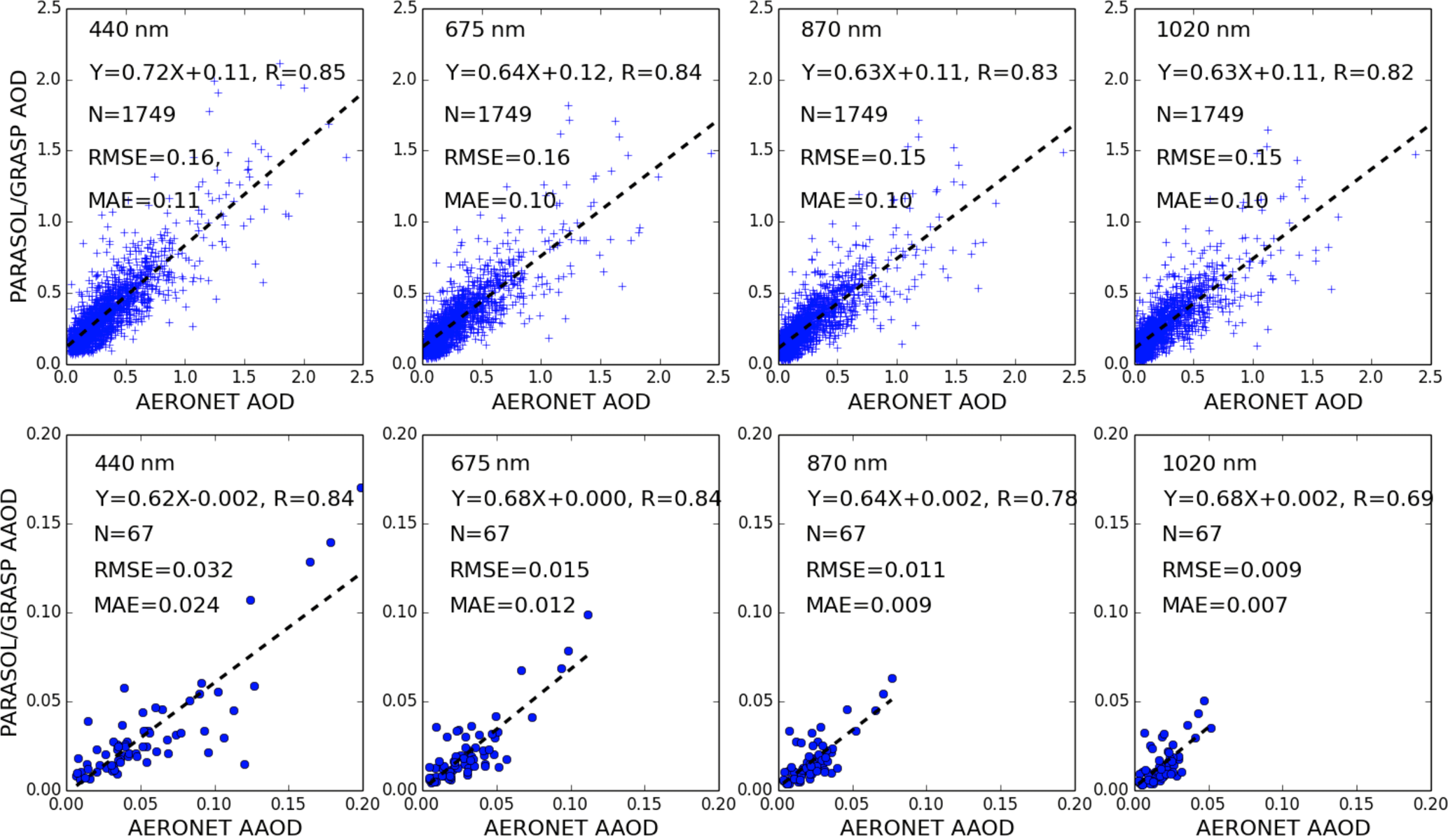
Figure 3Validation of 1 year of PARASOL/GRASP spectral AOD and AAOD re-scaled to 2.0∘ × 2.5∘ horizontal resolution with 28 AERONET site measurements at 440, 675, 870 and 1020 nm wavelengths over the study area; the number of matched pairs (N), correlation coefficient (R), root-mean-square error (RMSE) and mean absolute error (MAE) are provided in the top left corner.
2.3 PARASOL/GRASP aerosol products
GRASP is a recently developed aerosol retrieval algorithm that processes properties of aerosol and land surface reflectance. The algorithm is developed for enhanced characterization of aerosol properties from spectral, multi-angular polarimetric remote-sensing observations (http://www.grasp-open.com/, last access: 16 August 2018) (Dubovik et al., 2011, 2014; Lopatin et al., 2013). The POLDER/PARASOL imager provides spectral information of angular distribution of both total and polarized components of solar radiation reflected to space. With the expectation of three gaseous absorption channels (763, 765 and 710 nm), the observations over each pixel include total radiance at six channels (443, 490, 565, 670, 865 and 1020 nm) and linear polarization among three channels (490, 670 and 865 nm). The value of viewing angle is similar for all spectral channels and varies from 14 to 16 depending on solar zenith angle and geographical location. Meanwhile, PARASOL provides global coverage about every 2 days. Comprehensive measurements (∼144 independent measurements per pixel) from PARASOL allow GRASP to infer aerosol properties including spectral AOD and AAOD, the particle size distribution, single-scattering albedo, spectral refractive index and the degree of sphericity (some description of GRASP aerosol products can be found in papers of Kokhanovsky et al., 2015, and Popp et al., 2016).
In this study, we adopt 1-year (December 2007 to November 2008) PARASOL products of spectral AOD and AAOD from GRASP to retrieve DD, BC and OC emissions over the study area (in Sect. 4). In order to evaluate the reliability of PARASOL aerosol products from GRASP, we compared PARASOL/GRASP retrievals with AERONET measured AOD and AAOD at four sun photometer channels (440, 670, 870 and 1020 nm) in Fig. 3. Here, we use level 2 AERONET version 2 data, which are cloud screened and quality assured (Smirnov et al., 2000). From all 1-year measurements collected from 28 sites, we extract data between 13:00 and 14:00 local time. This provides a 60 min window centred at the PARASOL over-passing time of ∼ 13:30 LT. The averaged AERONET sun-direct AOD and AAOD by inversion of almucantar measurements (Dubovik et al., 2000; Dubovik and King, 2000) over this 60 min window are averaged for comparison with PARASOL/GRASP retrievals. We aggregate the PARASOL/GRASP products into 2∘ latitude × 2.5∘ longitude horizontal resolution to match the spatial resolution used by GEOS-Chem; any 2∘ × 2.5∘ grid box with less than 500 available PARASOL/GRASP retrievals for averaging is omitted. Depending on geographical location, the number of GRASP retrievals in a single 2∘ × 2.5∘ grid box ranges from 500 to 1600. Figure 3 presents the validation of retrieved PARASOL AOD and AAOD by the GRASP algorithm against the AOD and AAOD measured by AERONET. There is a solid correlation between PARASOL/GRASP and AERONET for AOD as well as AAOD. For example, the correlation coefficients (R) are 0.85 and 0.84, the RMSEs are 0.16 and 0.032, and the mean absolute errors (, where sums are over the ensemble of AOD and AAOD observations i, and Mi and Oi are the PARASOL/GRASP and AERONET values) of 0.11 and 0.024 for AOD and AAOD at 440 nm respectively.
3.1 Description of inverse modelling
Our inverse modelling approach optimizes BC, OC and DD emissions at the 2∘ × 2.5∘ horizontal resolution of the forward GEOS-Chem model, driven by GEOS-5 meteorological fields with 6 h temporal resolution. Overall, it follows the assimilation concept described in many textbooks and articles (e.g. Talagrand and Courtier, 1987 and Bennett, 2002). The details of specific realization of the approach used here are discussed in the details by Henze et al. (2007) and Dubovik et al. (2008).
The algorithm iteratively seeks adjustments to emissions in order to minimize the differences between observations and simulations as quantified by the cost function, J given by the sum of following quadratic form:
The first term characterizes the fitting of observations, where the vector fobs is the vector of observed values used for inversion and f(S) is the vector of simulated values based on emission sources S, while the vector S generally describes the four-dimensional distribution of emissions. Cobs is the error covariance matrix of fobs. The second term is introduced to constrain retrieval and it indicates the agreement with a priori estimates Sa of the emissions. Ca is the error covariance estimate of a priori emissions. Indeed, in general the information content of observations is insufficient for unique retrieval of all parameters describing emissions, i.e. the problem is ill-posed and some a priori information is needed. In most applications “prior model” emissions from bottom-up inventories Sa (i.e. standard model emissions) are used as a priori estimates of fundamentally unknown emissions. γr in Eq. (3) is a regularization parameter that is used for empirical adjustments of a priori term weight (see below).
The minimization of the quadratic form given by Eq. (3) can be obtained with steepest descent iterations:
where Kobs denotes the matrix of Jacobians of observation characteristics f. Equations (3) and (4) are written using vectors and matrices, describing four-dimensional geophysical fields that are generally very large. However, in practice neither transport models nor inverse modelling algorithms (if emissions retrieved at high resolution) explicitly utilize matrix and vectors. The transport models are generally organized as routines calculating continuous (i.e. with a relatively small time step) time series of the geo-characteristic resulting from time integration. For example, calculations of corrections ΔSp are obtained by running the adjoint model that directly produces the product of without explicit calculation of the Jacobians Kobs. For example, for inversion of observations of aerosol mass, i.e. f=m, the computations of gradient ∇Jp(t,x) of cost function Jp(t,x) using the adjoint model can be expressed as a time integration operation (see derivations by Dubovik et al., 2008) as follows:
where
and T represents transport operator. T and m are explicit functions of time t and spatial coordinates . T#(t,x) is the adjoint of the transport operator of T(t,x) (the adjoint operation is a transformation of the continuous function equivalent to matrix transposition operations) that is composed of adjoints of the component processes Ti(t,x):
The above equations describe an approach to invert the transport model based on the measurements of aerosol mass mobs, which is the direct simulation parameter in the CTM. In our analysis, the aerosol data fields are available only in the form of AOD and AAOD from the satellite measurements:
where f(…) is a function converting aerosol mass m(t,x) to AOD and AAOD using spectral aerosol extinction Qext(λ) and absorption Qabs(λ) coefficients, etc.; see in Eqs. (1)–(2). The correction minimizing the form of Eq. (3) that relates to fitting of AOD and AAOD under a priori constraints can be written as
Here is the adjoint operator corresponding to matrix operation FT, where matrix F contains first derivatives dτ∕ dm. It should be noted that the GEOS-Chem adjoint model is developed for inversion of mass (or AOD at a single wavelength); therefore the operator for inversion of spectral AOD and AAOD was developed as a part of this work.
In principle, the methodology assumes that the a priori information is available, i.e. before the inversion, which here is the default model emissions. Unfortunately, the covariance matrix Ca of a priori emissions is not accurately known. As a result, this matrix is often assumed to be diagonal, where the elements of diagonal are equal or defined using rather simple strategies. In addition, in order to address this fundamental lack of knowledge of Ca, the contribution of the a priori term (second term) in Eq. (3) is weighted by a regulation parameter, γr that is determined by empirical tests. This strategy is adapted here.
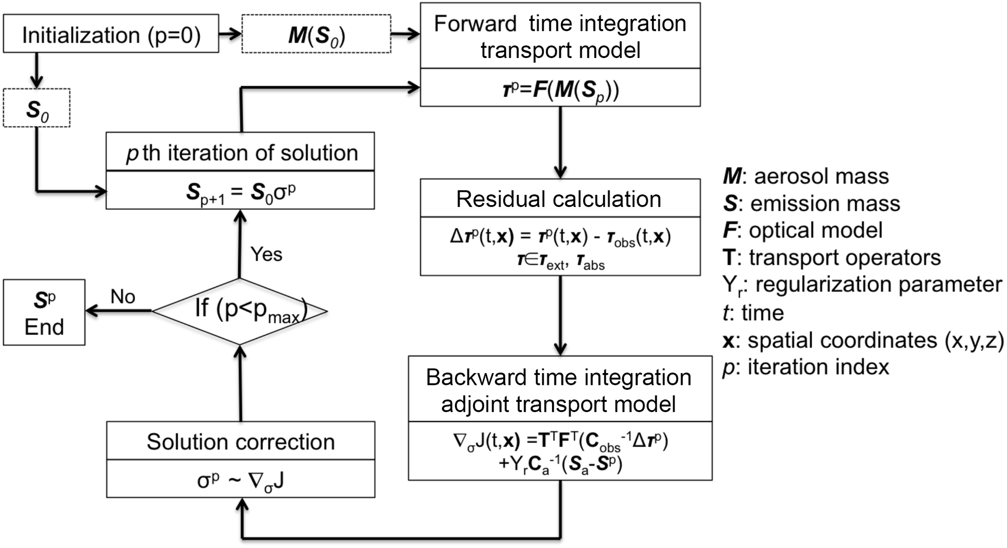
In addition, the GEOS-Chem adjoint model has been previously used for calculation of the gradient of Eq. (9) with respect to a vector of emissions scaling factors (Henze et al., 2007). While the scaling factor formulation had the advantage of replacing addition or subtraction correction of emissions (that can generate negative unphysical values) by division or multiplication of initial positive and non-zero S, this can be realized in the inversion algorithm by transforming into the log scale (see discussion by Dubovik and King, 2000, Dubovik, 2004 and Henze et al., 2009). However, the latter approach is rather challenging and GEOS-Chem used in this study relies on an empirically elaborated procedure (using equivalence . Specifically, from the gradients of cost function with respect to aerosol emission scaling factors ∇σJ(t,x), the adjoint GEOS-Chem uses the L-BFGS-B (quasi-Newton limited-memory Broyden–Fletcher–Goldfarb–Shanno with boundaries) optimization method (Byrd et al., 1995; Zhu et al., 1997), which affords bounded minimization of cost function and ensures positive values, to calculate the scaling factors for aerosol emissions. Figure 4 is the flow chart to illustrate the methodology.
In order to optimize the specification of a priori constraints and an initial guess, a number of synthetic tests were carried out in Sect. 3.2. It should be noted that using an a priori estimate of emission S0 is not the only way of adding a priori constraints in the inverse modelling. For example, Dubovik et al. (2008) demonstrated use of a priori knowledge on spatial and temporal variability in emissions, i.e. a priori limitation on derivative of corresponding functions (smoothness constraints). The potential advantage of smoothness constraints is that these limitations are milder than direct assumptions about values of emissions and therefore they introduce fewer systematic errors in the retrieval. However, such constraints are not used in this study.
3.2 Inversion test using synthetic measurements
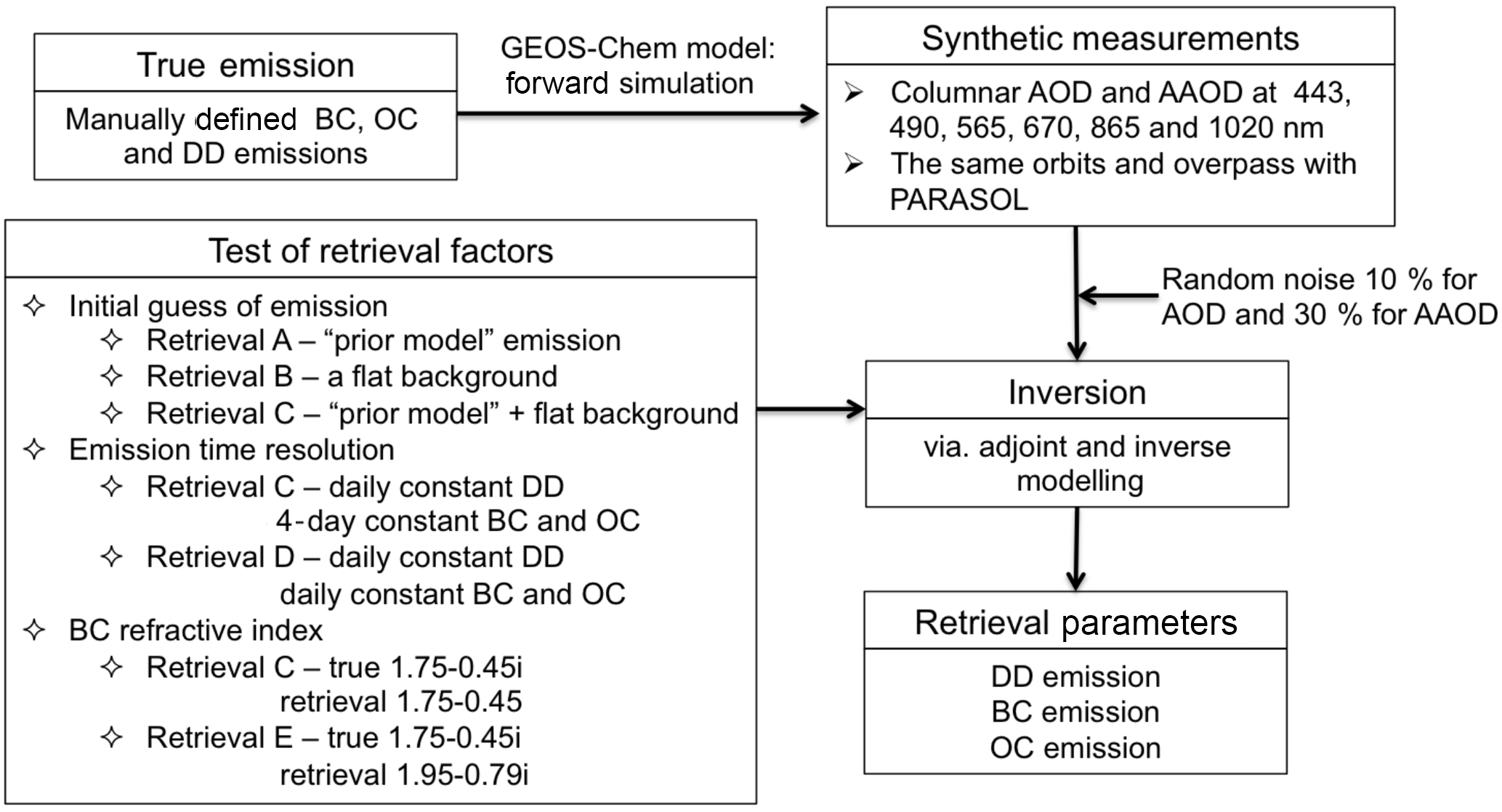
In this section, a series of numerical tests were performed to verify and illustrate how the algorithm inverts the synthetic measurements and to tune the algorithm settings (e.g. initial guess, emission correction time resolution and BC refractive index). The retrieved results were compared with “true emissions”. Synthetic measurements are PARASOL-like spectral AOD and AAOD at six PARASOL wavelengths, simulated from 16 days of BC, OC and DD emissions, which, for simplicity, are specified to be constant over the 16 days, yet different from the prior model emissions in order to test the algorithm performance under the circumstance that a priori knowledge of the emission distribution is limited. Figure 5 shows the design of the inversion test from synthetic measurements.

Figure 6Iterative comparison of spectral AOD and AAOD residual with two spectrum weight options.
3.2.1 Assumption of Cobs, definitions of spectral weights in AOD and AAOD fitting
In our inversion framework, the observed aerosol parameters contain AOD and AAOD at six PARASOL wavelengths. In principle, the weighting of observations of AOD and AAOD at these different wavelengths should be defined as . However, at present PARASOL/GRASP does not provide a covariance matrix Cobs for operational retrieval because it is computationally expensive and methodologically challenging. Indeed, GRASP simultaneously inverts a large group of pixels and the covariance matrix should be joint, i.e. characterize all inverted data. Such a matrix can be very large and it may have non-zero non-diagonal elements that are very difficult to use in practical applications. At the same time, GRASP AOD and AAOD were extensively evaluated against AERONET and there is overall understanding of accuracy. For example, usually AOD is about 10 times higher than the AAOD at the same wavelength (AAOD ∕ AOD = 1.0-SSA = ∼0.1). Therefore in order to make a contribution to the cost function, the AAOD is expected to be fitted about 10 times more accurately than AOD on an absolute scale. In addition, AAOD becomes very small at longer wavelengths. Based on these simple considerations we have defined different weighting for AOD and AAOD at different wavelengths. We have also assumed that retrieved AOD and AAOD are independent; i.e. Cobs is diagonal. Under such an assumption the absolute values of the Cobs diagonal are not of importance since the minimization procedure searches for the minimum and does not require knowledge of the cost function absolute value. In order to perform some optimization of fitting weights, we have performed several sets of tests to optimize the fitting weights of observations. Specifically we have performed the retrievals with different assumptions and analysed the goodness of fit. The spectral residual values to characterize the quality of spectral AOD and AAOD fit were defined as
The values of the spectral residuals RAOD(λ) and RAAOD(λ) are calculated after each iteration. The following options were tested using well-known qualitative tendencies. In a sensitivity test, two scenarios of spectrum weights are analysed. Since we are fitting the absolute value of AOD and AAOD, the relative accuracy of retrieved AOD and AAOD (Δτ∕τ and Δτa∕τa) is expected to be the same. The spectrum weights are defined as follows.
-
Option A. Unity weights (the elements of for AOD and AAOD are at six wavelengths: for AOD and for AAOD.
-
Option B. Unity weights for AOD but with more weights on AAOD are as follows: for AOD and for AAOD.
The retrievals are conducted with Option A and Option B (the inversion is conducted under Retrieval C scenario; see in the following sections), with other settings held constant. Comparison of spectral residuals after 20 iterations are shown in Fig. 6, which indicates that Option B has a better fit for AAOD than Option A by increasing the weights for AAOD, although spectral AOD can be fitted comparably well using either option.
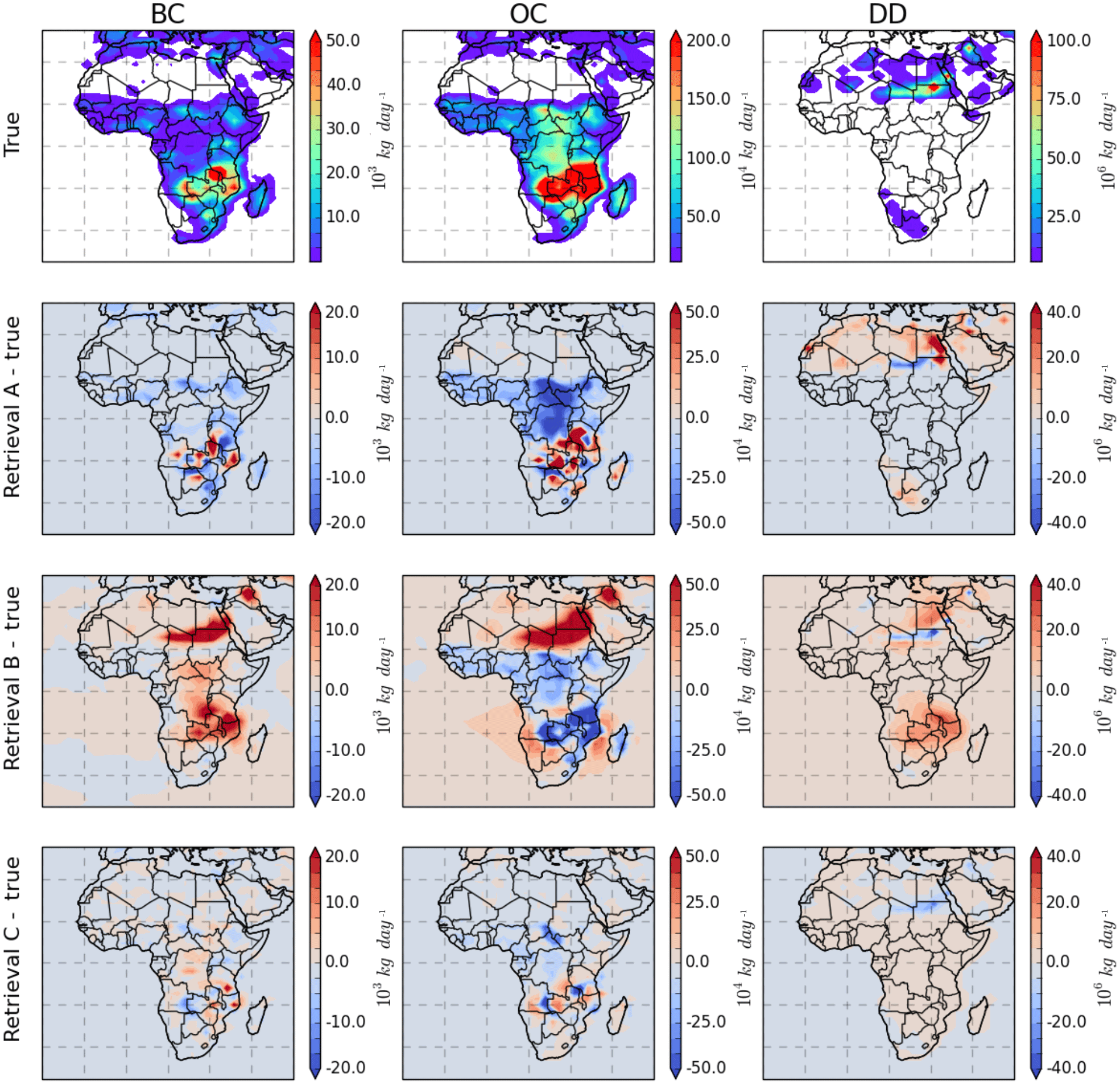
Figure 7Inversion test for retrieving BC, OC and DD emissions from synthetic measurements with three different initial guess schemes: (A) prior model emissions – Retrieval A; (B) spatially uniform – Retrieval B; (C) prior emissions with spatially uniform background – Retrieval C.
In future studies, it is expected that more adequate information for Cobs of PARASOL/GRASP AOD and AAOD will be available and it will be accounted for in future studies.
3.2.2 Effect of initial guess in emission retrieval
As mentioned in Sect. 3.1, the emission retrieval is an ill-posed problem and utilization of a priori constraints and initial guesses are essential factors for the retrieval. In our retrieval framework, the emissions are adjusted using scaling factors for an initial guess of emissions, S=S0σ. In principle, if the inverse problem is well constrained the solution should be independent of the initial guess. Therefore, we analyse the dependence on an initial guess using different retrieval settings. The inversion is conducted with three different initial guess schemes that we describe in detail in the following sections. In each of these three schemes, the input synthetic measurements are six wavelengths of AOD and AAOD, and the spectrum weights use the Option B scenario, while the retrieved emission correction time variations are assumed to be a daily constant for DD and a 4-day constant for BC and OC (note that we will separately test the assumption of emission correction time resolution in Sect. 3.2.3). Figure 7 shows the true emissions of DD, BC and OC and also the difference between true and retrieved emissions from three different initial guess schemes (Retrieval A, Retrieval B and Retrieval C). Figure 8 shows the scatter plots among BC, OC and DD emissions retrieved from Retrievals A, B and C versus true values.
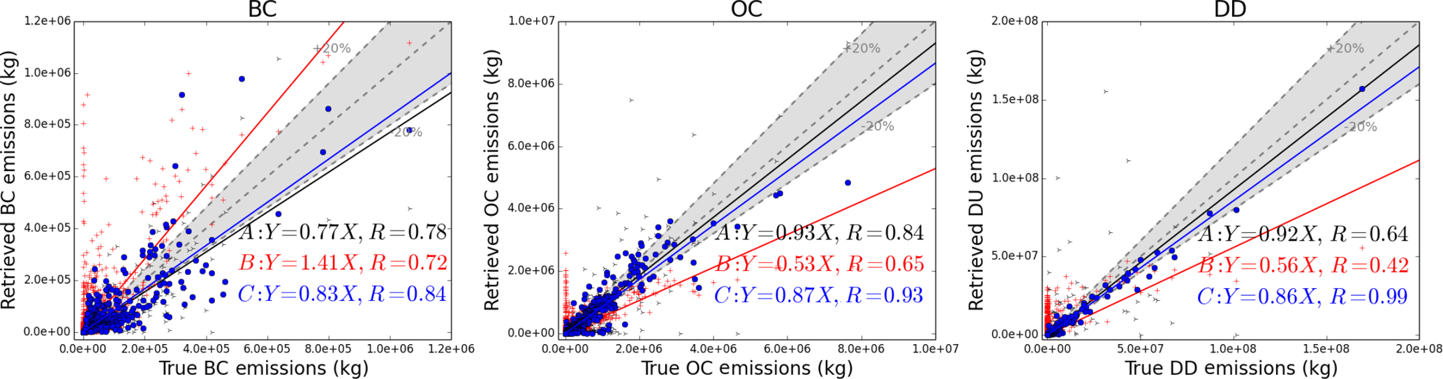
Figure 8Scatter plots among BC, OC and DD emissions retrieved from Retrievals A, B and C versus true values.
Thus, the following tendencies were observed in the conducted test.
A. Prior model: initial guess is equal to prior model emissions
In this method, the prior model emissions are directly used as the initial guess; therefore the adjustments of emissions are limited to the grid boxes with prior model emissions S0>0. At the same time, the true emissions have a difference with the prior model. The top row in Fig. 7 shows the assumed true BC, OC and DD emission distributions (units: kg day−1). The second row “Retrieval A – True” shows the differences between retrieved and true emissions from Retrieval A.
For Retrieval A, the retrieval highly relies on the accurate distribution of model prior emissions because the retrieval can only adjust the emissions on the grid boxes in which the model prior emissions are non-zero, and thus the retrieval could not create new sources. In our inversion test, the model prior emissions are different from the truth both for distribution and strength. Therefore, as shown in Fig. 8, Retrieval A produces overestimations over the grid boxes for which S0>0, while Strue=0; here Strue represents true emissions. However the underestimations occur over the grid boxes for which S0=0, while Strue>0.
B. Flat background everywhere
For Retrieval B, we investigate the use of spatially uniform initial guesses for the emissions. With this initialization, we allow BC, OC and DD emissions to be generated everywhere over land and ocean. In addition we are not using a priori knowledge of aerosol emissions. From the third row “Retrieval B – True” Fig. 7, the algorithm can determine the intensive aerosol emission grid boxes, in which high aerosol loading is observed. However, the desert dust and carbonaceous aerosol sources were not correctly reproduced since a uniform emission is used everywhere. The scatter plots between retrieved emissions from Retrieval B and true values are also shown in Fig. 8. In this case, the retrieval could produce overestimations over some grid boxes in which Strue=0. Although the uniform emission assumption gives the algorithm more freedom to find new sources, our tests indicate that the retrieval could produce false sources in this assumption when the algorithm tries to determine BC, OC and DD emissions simultaneously. This misrepresentation indicates that the spectral AOD and AAOD are not sufficient to identify BC, OC and DD emissions without any a priori knowledge.
C. Prior model emissions with flat background
In Retrieval C, the retrieval was initiated using prior model emissions but including a spatially uniform value over land grid boxes in which S0=0. In this study, the flat values equal to 10−4 Tg day−1 grid−1 for DD, 10−6 Tg day−1 grid−1 for BC and Tg day−1 grid−1 for OC are used, which account for ∼5% of the true emissions over the entire area. This assumption allows the retrieval of BC, OC and DD aerosol emissions everywhere over land (ship emissions over ocean are included in the model prior emissions), and at the same time it uses prior emission constraints to prevent false source generation that could occur due to inaccuracies in data or model processes. Figures 7 and 8 show that overall Retrieval C captures the emission distributions more accurately than Retrieval A and Retrieval B. The average ratio of retrieved emissions to truth ( for Retrieval C is 1.02±1.05 for BC, 0.87±1.42 for OC and 1.24±1.80 for DD.
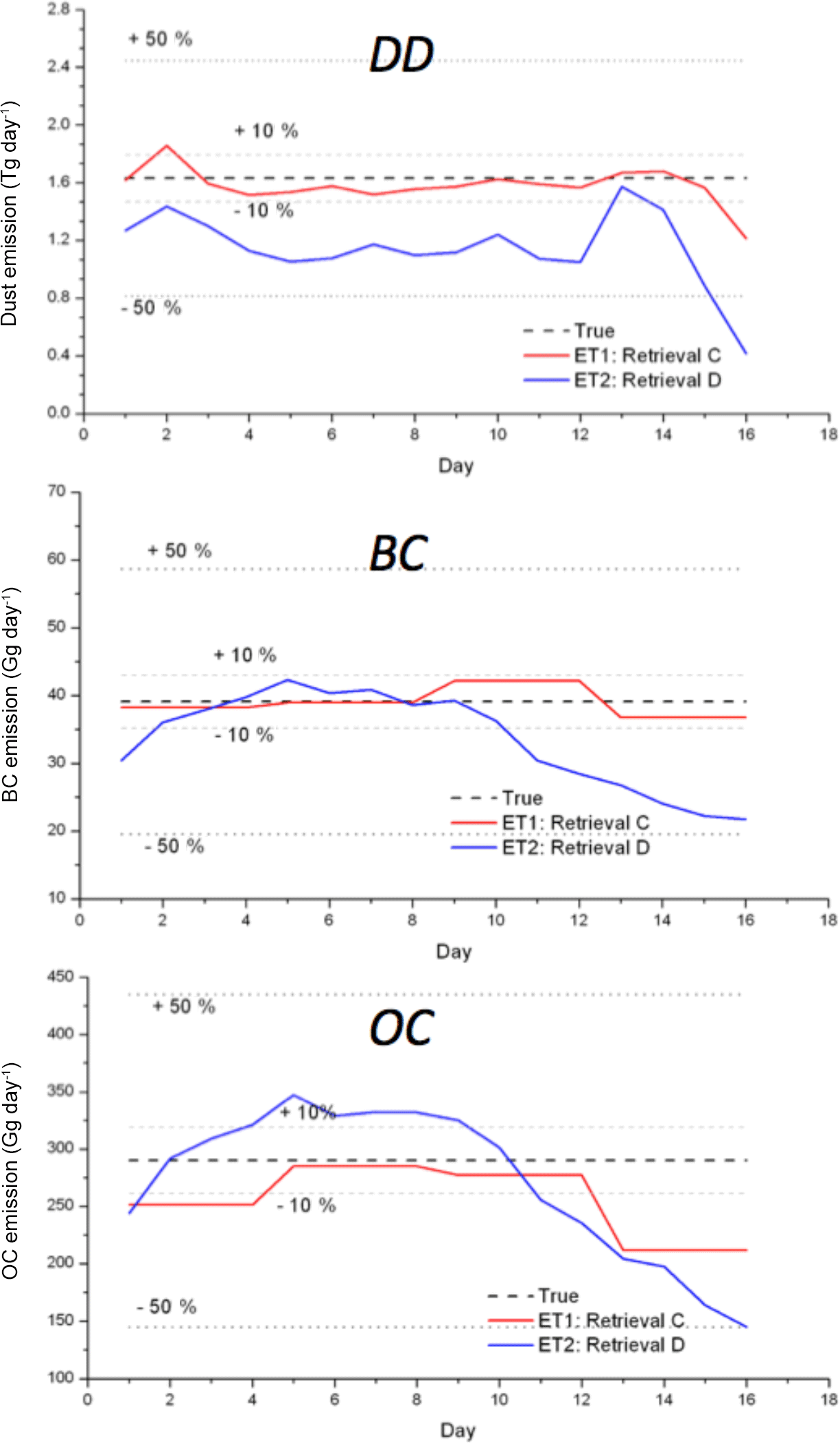
Figure 9Sensitivity test for retrieving DD, BC and OC emissions over 16 days with two scenarios of assumption of emission correction time resolution.
3.2.3 Assumption of emission correction time resolution
Aerosol sources are known to have high temporal and spatial variability. However, because PARASOL observations have limited temporal coverage (e.g. ∼2 days global coverage, with observations once per day), the variability in aerosol emissions at any given location can only be retrieved at a frequency of no more than once per day. In order to investigate how assumptions regarding temporal variability in emissions can affect the retrieval, we repeat the retrieval using two scenarios for emission correction: ET1, daily correction constant of DD, BC and OC emissions, and ET2, daily correction constant of DD emissions and 4-day correction constant of BC and OC emissions. For each scenario, the input observations are six wavelengths of AOD and AAOD, and the retrieval is initialized by prior model emissions with a uniform background emissions (Retrieval C). Two scenarios are used. We test these two scenarios by conducting a 16-day retrieval, and Fig. 9 shows the comparison among retrieved daily total DD, BC and OC emissions with the true emissions. Note that the ET1 scenario uses the same settings as Retrieval C in Sect. 3.2.2, and ET2 is named Retrieval D.
Figure 9 shows the retrieval maximum uncertainty for total daily DD emissions over the study area is within 25.8 % for Retrieval C; however this value reaches more than 50 % for Retrieval D. For BC, the maximum uncertainty is within 5.9 % for total daily emissions from Retrieval C, while it reaches up to 40.8 % for Retrieval D. The uncertainty of daily OC emissions is within 26.9 % for OC using Retrieval C, while it is about 38.6 % for Retrieval D. Overall, from this sensitivity test, the Retrieval C shows a better capability to capture the spatial distribution of DD, BC and OC emissions than Retrieval D, and it does not introduce false temporal variability.
It should be noted that the regularization parameter defining the contribution of the a priori term in all tests was chosen to be very small (i.e. 0.0001) in order to make the retrieval rely mostly on the observations. Thus, the good convergence to the sought solution was obtained with minimum constraints. It is planned to investigate this aspect in future studies.
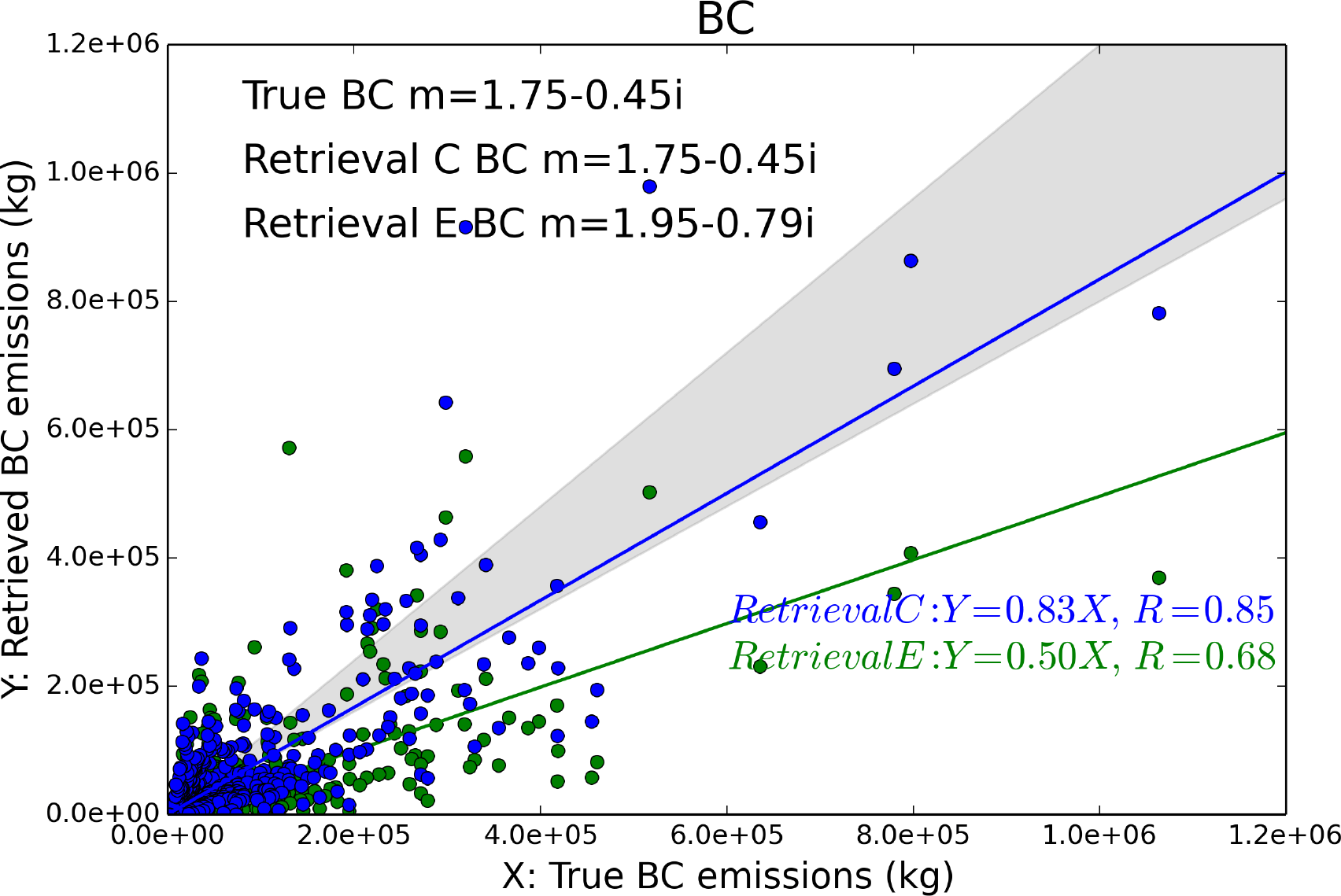
Figure 10Test of BC particle refractive index influence on the retrieval of BC emissions. The scatter plots are a grid-to-grid comparison of retrieved 16-day averaged emissions (blue: Retrieval C; green: Retrieval E) with the “true” BC emissions. The shaded grey area represents ±20 % differences around the true values.
3.2.4 Uncertainty in assumption of BC refractive index
Aerosol particles' light scattering and absorption efficiencies are determined by their complex refractive indices, expressed as , where n is the real part and k is the imaginary part. The real part of the complex refractive indices defines the light scattering property of an aerosol species, whereas the imaginary part of the complex refractive indices determines the absorbing ability. Black carbon aerosol is the strongest atmospheric absorber of solar radiation. Its imaginary refractive index is at least about 2 orders of magnitude higher than other aerosol species (see Table 1). To identify the impact of the uncertainties of BC refractive index in our results, we test another commonly used specification of 1.95–0.79i (Bond and Bergstrom, 2006) in our retrieval scheme (denoted as Retrieval E). Figure 10 compares the BC emission results from Retrieval E and Retrieval C (where the BC refractive index of 1.75–0.45i (Hess et al., 1998) was used) with the true BC emissions.
The synthetic measurements of AOD and AAOD are simulated with a BC refractive index m=1.75-0.45i, and the scenario Retrieval C uses the retrieval with the same BC refractive index; the slope of linear regression between the resulting retrieved and true BC emissions is 0.83, and the retrieved BC emissions over the study area is 39.0 Gg day−1. In contrast, the Retrieval E scenario uses the retrieval with a higher BC absorption and scattering definition, m= 1.95–0.79i, and as expected we obtain lower magnitudes of BC emissions (21.8 Gg day−1), and the slope between retrieved and true BC emissions decreases to about 0.5. This sensitivity test demonstrates that uncertainty in the BC refractive index can lead to a factor of about 1.8 in total BC emissions.
Overall, these sensitivity tests suggest that our inversion scheme is capable of determining the strength and spatial distribution of BC, OC and DD emissions simultaneously from the multispectral PARASOL/GRASP AOD and AAOD products in the following manner.
-
Six wavelengths (VIS–NIR) of AOD and AAOD from PARASOL/GRASP are needed to retrieve BC, OC and DD emissions simultaneously.
-
The weighting spectral factors for the PARASOL six wavelengths ( for AOD and for AAOD) were optimized to provide an improved fit of both spectral AOD and AAOD.
-
The BC, OC and DD emissions are allowed everywhere over land. The retrieval is initialized by prior model emissions with a uniform background. The retrieval with this initialization could detect new sources and perform satisfactorily even when a priori knowledge of aerosol emissions is not fully consistent with the assumed emissions. This scenario will be used in Sects. 4 and 5.
-
The emission corrections are assumed to be daily constant for DD and 4-day constant for BC and OC. Owing to the limited observations available for assimilation, this assumption helps to make the retrieval sufficiently accurate and stable with a rather generic initial guess.
-
The BC emission retrieval is sensitive to BC refractive index assumption, which could produce a factor of ∼1.8 difference between the two sets of commonly used BC refractive index data for total BC emissions. We will produce two BC emission datasets with two scenarios of BC refractive index, Case 1: m= 1.75–0.45i and Case 2: m= 1.95–0.79i.
In this section, we discuss retrieval of DD, BC and OC emissions simultaneously from the actual PARASOL/GRASP spectral AOD and AAOD data from December 2007 to November 2008. The SU and SS aerosol simulations are kept as the prior model. PARASOL/GRASP retrievals were aggregated to the same horizontal resolution as the GEOS-Chem model (2∘ × 2.5∘) and averaged within the grid cells prior to assimilation. When iteratively minimizing Eq. (3), the maximum iteration number was chosen to be 40, which takes about 60 days to complete on a computer workstation with 32×3.3 GHz CPUs. Based on conducted tests, the decrease in the cost function is very minor starting from the 20th iteration (e.g. see Fig. 6).
4.1 Fitting of aerosol optical depth
One of the important indicators of our inversion performance is the fitting of PARASOL/GRASP spectral AOD and AAOD. We evaluate the GEOS-Chem-simulated spectral AOD at 443, 490, 565, 670, 865 and 1020 nm using prior or posterior emissions against the corresponding PARASOL/GRASP-retrieved AOD in Fig. 11. The posterior GEOS-Chem spectral AODs are simulated using retrieved DD, BC and OC emissions, which will be presented in Sect. 4.2. Figure 11a presents the annual average of the PARASOL spectral AOD from the GRASP algorithm, whereas Fig. 11b and c show the same quantity from the GEOS-Chem simulations with prior and posterior emissions, respectively. Here we extract GEOS-Chem hourly AOD with the same PARASOL orbit partition at 13:00 LT, which is approximately the PARASOL overpass time of 13:30 LT. Figure 11d and e display the grid-to-grid comparison between PARASOL/GRASP spectral AOD and prior and posterior GEOS-Chem simulation during 1 year, colour-coded with the PARASOL Ångström exponent . The Ångström exponent α is often used as a qualitative indicator of aerosol particle size; the smaller the α, the larger the particle size. For example, the α values for “pure” dust aerosols are usually near zero, whereas that for smoke or pollution aerosols are generally greater than 1 (Eck et al., 1999; Schuster et al., 2006).

Figure 11Comparison of the annual spatial distribution of prior (b) and posterior (c) GEOS-Chem-simulated AOD at 443, 490, 565, 670 865 and 1020 nm with PARASOL/GRASP observations (a). The posterior spectral AODs are simulated using retrieved DD, BC and OC emissions. The scatter plots are grid-to-grid comparisons between PARASOL/GRASP spectral observations versus prior (d) and posterior (e) GEOS-Chem simulations during 1 year. The correlation coefficient (R) and root-mean-square error (RMSE) are provided in the top left corner.
One of the major discrepancies between the prior GEOS-Chem simulation and PARASOL/GRASP observation is that the model produces the highest annual average AOD values over the major dust source region of northern Africa; however, satellite data show the maxima AOD in central and the southern Africa, where carbonaceous aerosols usually dominate (although central Africa may also be influenced by dust events). Hence, compared to PARASOL/GRASP observations, the prior GEOS-Chem AOD is overestimated in northern Africa, while it is underestimated in the southern Africa biomass burning and Arabian Peninsula regions. Some recent studies by Ridley et al. (2012, 2016) and Zhang et al. (2015) also indicate that the GEOS-Chem model overestimates dust AOD in northern Africa. Meanwhile, Ridley et al. (2012) and Zhang et al. (2013) propose a new and realistic dust particle size distribution according to the measurements from Highwood et al. (2003), which can partially adjust the misrepresentation of dust near the source and over transport areas. This new particle size distribution has been adopted in our prior and posterior GEOS-Chem simulation. In addition, the underestimation of model-simulated AOD in biomass burning regions with the GFED emission database was also shown in other modelling studies (Chin et al., 2009; Johnson et al., 2016). The model-simulated spectral AODs with the posterior emissions agree with the PARASOL observations much better, in spite of slight systematic overestimations from 565 to 1020 nm (about 13 % on an annual average). This overestimation indicates some disagreement in modelling of AOD for these bands that needs to be investigated and addressed in future studies.
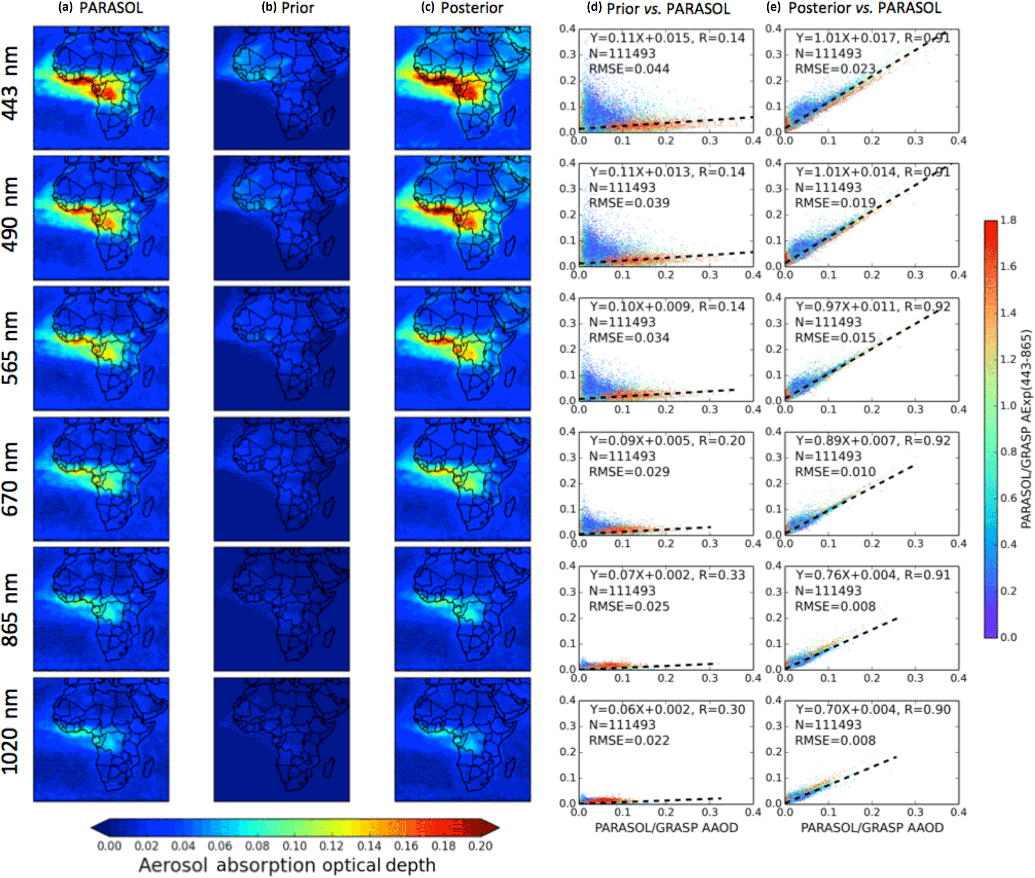

Figure 13Comparison of monthly total DD, BC and OC emissions (unit: Tg) over the study area between prior model (GFED3 and Bond inventories for BC and OC, DEAD model for DD) and retrieved emissions; the annual values (unit: Tg yr−1) are provided in the top left corner.
Figure 11d and e show the statistics of prior and posterior GEOS-Chem-simulated AOD versus PARASOL/GRASP observed AOD at six wavelengths during the entire year. The number of matched pairs is 111 493. For the GEOS-Chem simulation with the posterior emissions, all the statistics parameters between model and observation are improved at all six wavelengths compared to the simulation with prior emissions. For example, the correlation coefficient has increased from 0.49–0.51 to 0.89–0.92 and the RMSE has decreased from 0.27–0.34 to 0.10–0.13. Such improvements are expected as the posterior emissions are retrieved based on the PARASOL/GRASP AOD data. We will show further evaluations with other datasets in Sect. 5.
4.2 Fitting of aerosol absorption optical depth
Similar to the AOD analysis, here we evaluate the fitting of AAOD (Fig. 12). From the annually averaged spectral AAOD in Fig. 12, the prior GEOS-Chem simulation (Fig. 12b) shows significant underestimations of AAOD over the entire domain compared to PARASOL/GRASP observations (Fig. 12a). Conversely, the posterior GEOS-Chem simulation (Fig. 12c) produces much better agreement with the PARASOL/GRASP data for all wavelengths, with a small overestimation of AAOD in the spectral range from 443 to 565 nm (about 6 % on annual average) and a small underestimation at 865 and 1020 nm (about 9 % on annual average). Linked with the ∼13 % overestimation of annual AOD from 565 to 1020 nm, this systematic phenomenon of fitting is possibly due to the model's relatively coarse-resolution results in misrepresentations of DD, BC and OC emissions in some grid boxes.
Figure 12d and e show the comparisons of PARASOL/GRASP-observed AAOD at six wavelengths with the corresponding GEOS-Chem-simulated quantities using prior or posterior emissions. The very low linear regression slope between the model-simulated AAOD using prior emissions with observations (less than 0.11 over all six wavelengths) indicates that the prior simulations significantly underestimate the AAOD. In contrast, model simulations with the posterior emissions improve the slope to 1.01 at 443 nm and 0.70 at 1020 nm. Similar to the case of AOD, the agreements between the PARASOL/GRASP AAOD data and the model simulations are much better using the posterior emissions than using the prior emissions, with the correlation coefficients increased from 0.14–0.33 to 0.90–0.92 and the RMSE decreased from 0.022–0.044 to 0.008–0.023.
4.3 Emission sources
The retrieved and prior monthly total DD, BC and OC emission variations over the study area are shown in Fig. 13.
4.3.1 DD emissions
Figure 13 shows that the retrieved annual total DD emissions in the study area is 701 Tg yr−1 (particle radius ranging from 0.1 to 6.0 µm, excluding super-coarse-mode dust particles), which is 45.7 % smaller than the prior emissions of 1291 Tg yr−1. Moreover, the retrieved total DD emissions show reduced emissions amount from the prior values in every month, varying from 11.6 % reduction in December to 68.5 % in May. Figure 14 shows the comparison of the spatial distribution of seasonal DD emissions between the prior emissions (Fig. 14a) and our retrievals (Fig. 14b). As shown in Fig. 14, the prior and the retrieved emissions show similar spatial and seasonal patterns; for example, the Bodélé Depression is the most active dust source area in DJF and SON and the Arabian Desert becomes active in MAM and JJA. One major discrepancy between the model and the retrieval is that the model has much stronger DD sources over Algeria and Morocco in MAM and JJA, which are even stronger than the Bodélé Depression and the Arabian Desert. However, the retrieval still shows the dust emissions there, while the strength decreases by a factor of 5–6.

Figure 14Spatial distribution of seasonal desert dust aerosol emissions: (a) “prior model” DD emissions from DEAD model and (b) retrieved DD emissions.
4.3.2 BC emissions
As mentioned earlier, we considered two cases of BC aerosol refractive index to perform the retrieval (Case 1: m= 1.75–0.45i; Case 2: m= 1.95–0.79i) since the retrieved total BC emissions are very sensitive to the BC refractive index (our sensitivity test shows a factor of ∼1.8 differences between Case 1 and Case 2; see Sect. 3.2.4). Figure 13 shows the retrievals increase BC emissions for every month from the prior emissions by factors ranging from 5.9 in March to 14.4 in November, with an annual averaged increase of a factor of ∼8 in Case 1. For Case 2, the retrieved BC emissions have similar monthly variation to in Case 1 with a smaller magnitude of increase from the prior emissions, from a factor of 3.3 in March to 4.7 in November with an annual averaged increase of ∼3.
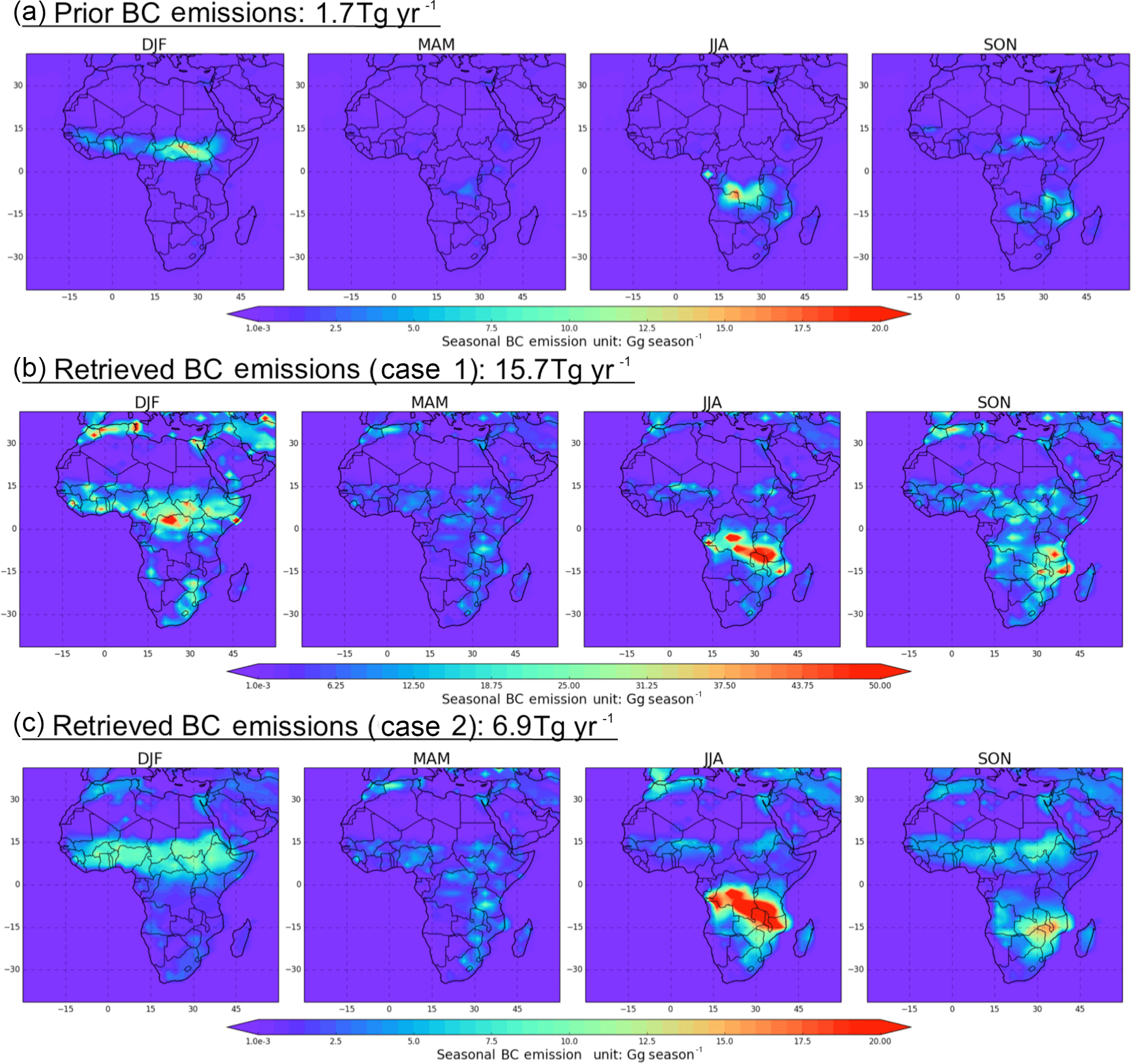
Figure 15Spatial distribution of seasonal BC emissions: (a) prior model BC emissions from GFED3 and Bond inventories; (b) Case 1 retrieved BC emissions; (c) Case 2 retrieved BC emissions. Note that the colour scale for (b) is different from (a) and (c) for better resolving the spatial contrasts.
The spatial comparison of seasonal BC emissions is summarized in Fig. 15. We plot model prior BC emissions from GFED3 and Bond anthropogenic inventories in Fig. 15a, retrieved BC emissions from Case 1 in Fig. 15b, and Case 2 retrieved BC emissions in Fig. 15c. Note that the colour bar range in Fig. 15b is 2.5 times larger than that of Fig. 15a and Fig. 15c. Not surprisingly, the patterns of model prior emissions in Case 1 and Case 2 retrievals are similar, with the highest BC emission source areas located in biomass burning regions, such as central Africa during DJF and southern Africa JJA. The large increases in the BC emissions in the retrieval relative to the prior suggest that the current model-simulated AAOD is much too low, which is consistent with the PARASOL/GRASP observations in Sect. 4.2. Retrieval Case 2 shows a large increase over the Arabian Peninsula, indicating there is an emission ∼5 times higher than the prior model in DJF, MAM and SON, for which the latter shows only a small amount of carbonaceous fine particles. AERONET ground-based measurements indicate a moderate absorption phenomenon there (seasonal AAOD at 550 nm about ∼0.05; see Fig. 21), which corroborates the retrieved values from the inversion.
4.3.3 OC emissions
The annual total OC emissions in Fig. 13 show that the retrieved annual OC emissions are higher than the prior model by a factor of ∼2, with a minimum monthly increase found in March (1.54) and a maximum in May (5.71). Combined with BC emissions, the retrieved total carbonaceous aerosol emissions are 52.8 Tg yr−1 (with Case 1 BC) and 44.0 Tg yr−1 (with Case 2 BC), which is 271.8 % (Case 1) to 209.8 % (Case 2) higher than the prior model (14.2 Tg yr−1). We compare the seasonal distribution of prior OC emissions with retrieved emissions in Fig. 16. Both the retrieved and prior emissions have the highest OC emissions in southern Africa in JJA and in central Africa in DJF.
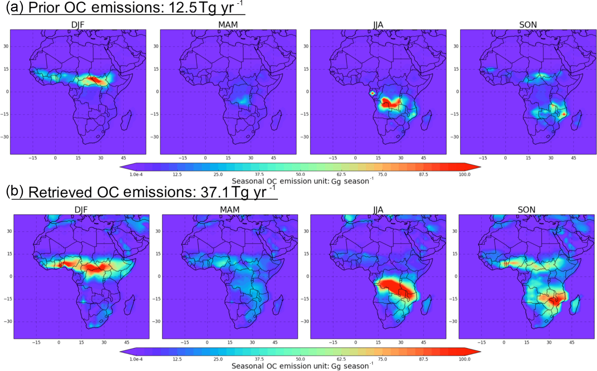
Figure 16Spatial distribution of seasonal OC emissions: (a) prior model OC emissions using GFED3 and Bond inventories and (b) retrieved OC emissions.
4.3.4 Summary of retrieved emissions
Comparison of retrieved DD, BC and OC aerosol emissions over the study area with the GEOS-Chem prior model emission inventories showing basically consistent spatial and temporal variation. However, the significant differences are in the emission strength. The PARASOL/GRASP-based retrieval reduces the GEOS-Chem annual DD emissions to 701 Tg yr−1 over the study area. A recent study by Escribano et al. (2017) estimated that the mineral dust flux for particle size of less than 6.0 µm over northern Africa and the Arabian Peninsula is between 630 and 845 Tg yr−1. Some other studies also show similar dust emission flux over Africa (Werner et al., 2002; Miller et al., 2004; Escribano et al., 2016, 2017). However, the overestimation of the prior model dust emissions could also result from errors in particle size distribution, which is shown to be biased toward smaller particle sizes compared to the observation in the atmosphere (Kok et al., 2017). Meanwhile, the retrieval increases the model annual carbonaceous aerosol emissions by about 2.5 times. This value is close to the recommendation given in Bond et al. (2013) to increase global BC absorption by a factor of 3 to fit the observation of columnar aerosol absorption. Kaiser et al. (2012) also recommend correcting the carbonaceous aerosol emissions (GFED3) with a factor of 3.4 when using them in the global aerosol forecasting system. In addition, there are many other efforts to improve the simulation of AAOD, e.g. treating hydrophilic BC as an internal aerosol core with other soluble hygroscopic aerosol species (Wang et al., 2016) and including light-absorbing brown carbon in the simulation (X. Wang et al., 2014). These studies are all crucial to improve current CTM aerosol simulation, which should be adopted in our aerosol emission inversion framework in the future.
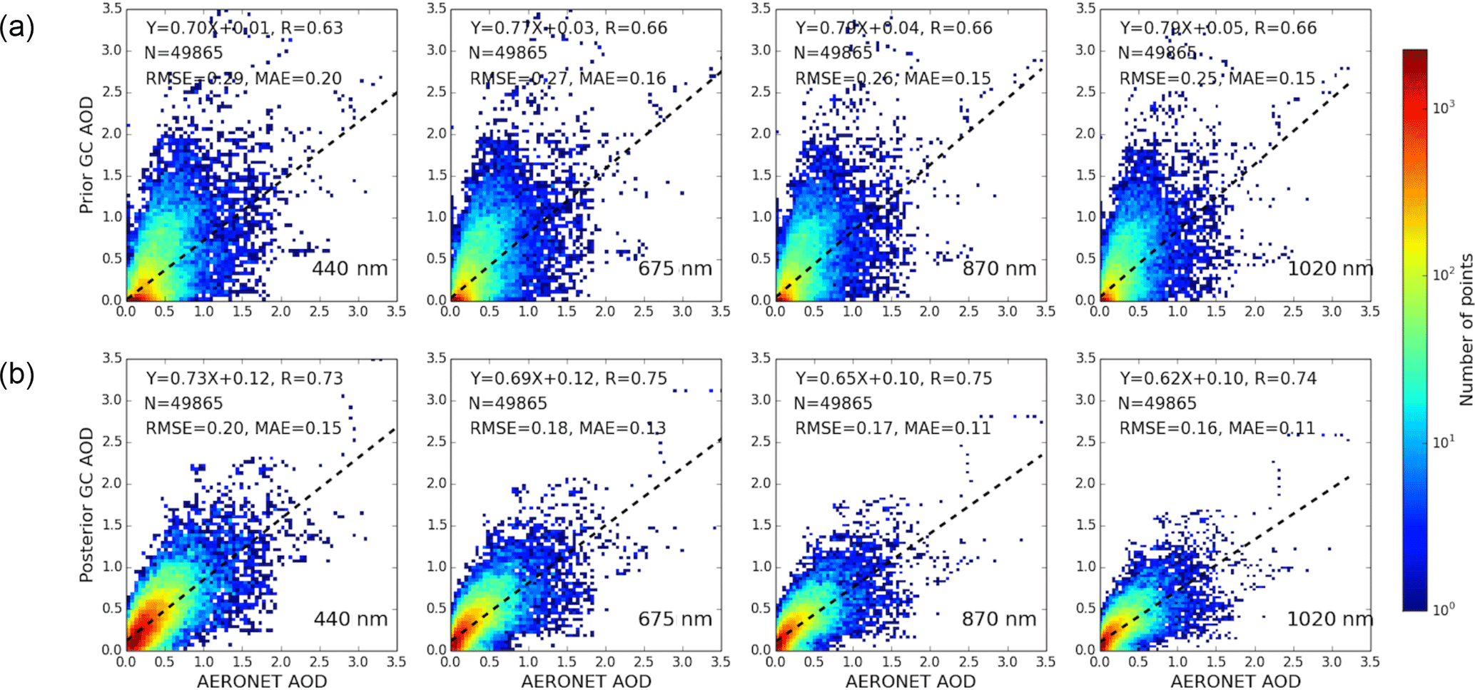
Figure 17Density scatter plots of 1-year GEOS-Chem-simulated AOD using the prior emissions (a) or the posterior emissions (b) versus AERONET-measured AOD at 440, 675, 870 and 1020 nm at 28 sites. The AOD data were aggregated into 80 bins for both the x and y directions spanning the range from 0.0 to 3.5 for AOD at four wavelengths. The number of matched pairs (N), correlation coefficient (R), root-mean-square error (RMSE) and mean absolute error (MAE) are shown on each panel.
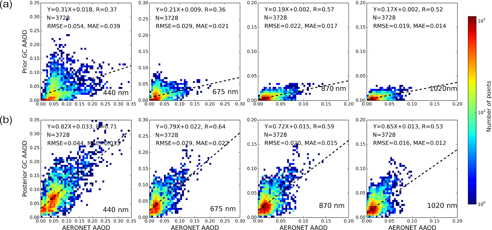
Figure 18Same as Fig. 17, but for AAOD. The AAOD data were aggregated into 50 bins for both the x and y directions spanning the range from 0.0 to 0.35 for AAOD at 440 nm, 0.0 to 0.3 at 675 nm, and 0.0 to 0.2 at 870 and 1020 nm.
5.1 Evaluation with AERONET
In order to objectively evaluate our retrieved aerosol emissions based on PARASOL/GRASP spectral AOD and AAOD, we made a series of evaluations using independent datasets and models not used by our inversion. First, the posterior simulated 1-year AOD and AAOD (using Case 1 BC emissions) are compared with the sun-photometer-measured AOD and AAOD at 28 AERONET sites (shown in Fig. 1).
Figures 17 and 18 show the comparison of GEOS-Chem simulations using prior and posterior emissions with AERONET measurements of AOD and AAOD, respectively. The evaluation was conducted at four wavelengths (440, 675, 870 and 1020 nm) and GEOS-Chem hourly spectral AOD and AAOD are interpolated based on the Ångström exponent. AERONET AOD and AAOD output averaged over time for ±30 min and centred by model are used to compare with the model simulations over the grid box containing the AERONET sites. Density scatter plots of 49 865 matched pairs of AOD are shown in Fig. 17. The correlation coefficients between GEOS-Chem simulations with prior emissions and AERONET data (shown in Fig. 17a) are 0.62, 0.67, 0.66 and 0.66 for the four wavelengths respectively, and the corresponding RMSEs are 0.28, 0.25, 0.24 and 0.24. Yet, the correlation coefficients are increased to 0.73, 0.75, 0.75 and 0.74 when the posterior emissions are used in the GEOS-Chem simulation (Fig. 17b), and meanwhile the RMSEs are decreased to 0.20, 0.18 0.17 and 0.16 respectively. Meanwhile, the mean absolute errors are also decreased from prior (0.20, 0.16, 0.15 and 0.15) to posterior (0.15, 0.13, 0.11 and 0.11).
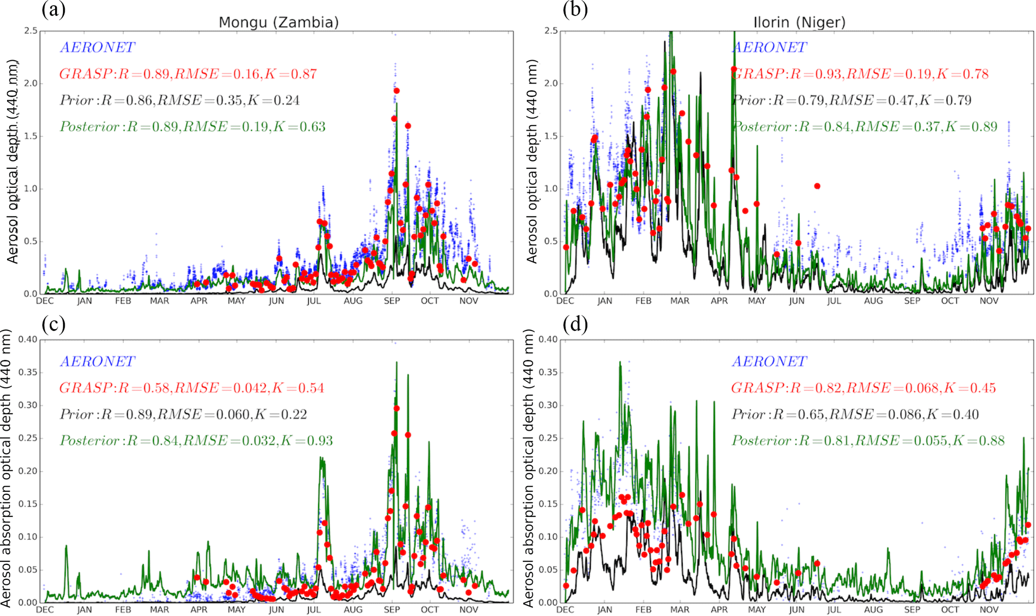
Figure 19Time serial AOD (a, b) and AAOD (c, d) from AERONET (blue crosses), PARASOL/GRASP (red circles), prior GEOS-Chem (black line) and posterior (green line) GEOS-Chem simulations at two sites (Mongu and Ilorin). The error statistics parameters between PARASOL/GRASP and prior and posterior GEOS-Chem simulations with AERONET are also shown in the figure.

Figure 20Comparison of the seasonal spatial distribution of prior (b) and posterior (c) GEOS-5/GOCART-simulated AOD at 550 nm with MODIS observations (a). The scatter plots of grid-to-grid comparison between MODIS and prior GEOS-5/GOCART AOD (d) and posterior GEOS-5/GOCART AOD (e) are also shown. The ground-based measurements from AERONET (squares) are over-plotted over panels (a)–(c). The MODIS and GEOS-5/GOCART versus AERONET correlation coefficient (R) and root-mean-square error (RMSE) are provided in panels (a)–(c). Meanwhile, the GEOS-5/GOCART versus MODIS R, RMSE and MAE are also provided in panels (d)–(e).
Figure 18 shows the density scatter plot comparisons for AAOD. However, unlike direct sun measurement of AOD, AERONET AAOD is inverted from almucantar measurements. To select sufficiently accurate retrievals, we applied standard quality screening criteria (e.g. Dubovik et al., 2002b and Holben et al., 2006). Therefore, there are fewer AERONET AAODs that matched with GEOS-Chem simulations than for AOD. The number of matched pairs is 3728. The low slope of the linear regression between prior model AAOD and AERONET (Fig. 18a) indicates that the prior model significantly underestimates AAOD. The posterior GEOS-Chem simulations using retrieved emissions (Fig. 18b) show the improvements validated with AERONET, with the correlation coefficients at 0.71, 0.64, 0.59 and 0.53. In addition, the RMSEs are also improved for posterior simulations.
Comparison between time series of AOD and AAOD at 440 nm from AERONET, PARASOL/GRASP, and prior and posterior GEOS-Chem simulations from December 2007 to November 2008 are made at two AERONET sites (Mongu and Ilorin), and the results are shown in Fig. 19. The geo-locations of these two sites are already apparent in Fig. 1. Ilorin is located close to the active dust sources in northern Africa, which are also influenced by seasonal biomass burning events, especially from November to February. Mongu is located close to the southern African seasonal biomass burning sources. The posterior simulations better capture the time series variations in and magnitude of AOD and AAOD from AERONET measurements. For example, in Mongu, the prior simulation underestimates AOD and AAOD significantly. In September, the underestimations are about 3 times (a bias of −0.56 for monthly average) for AOD and 4 times for AAOD (a bias −0.09). Such bias is significantly reduced to −0.22 for AOD and +0.01 for AAOD in the posterior simulation with retrieved emissions. In terms of correlation coefficients, the prior GEOS-Chem simulation shows a solid correlation with measurements in Mongu, while the slope of the linear regression (K) between the prior simulation and AERONET (0.24 for AOD; 0.22 for AAOD) indicates that the model significantly underestimates the aerosol loading in Mongu. Furthermore, prior GEOS-Chem simulation can capture the variation in and magnitude of AOD (R=0.79 and K=0.79) in Ilorin. However, for AAOD, the simulation shows underestimation with a slope K=0.40, which is an indicator of the model underestimation of the aerosol absorption species, such as BC. Overall, the posterior GEOS-Chem simulation with retrieved emissions can better capture the time serial variation in and magnitude of AOD and AAOD in both Mongu and Ilorin.
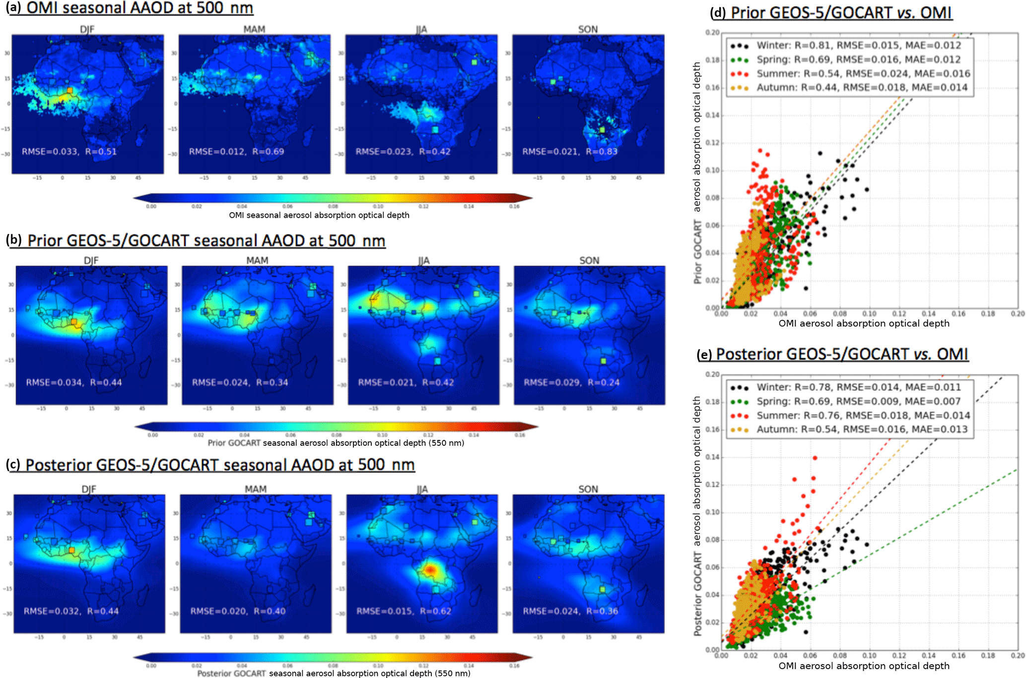
Figure 21Comparison of the seasonal spatial distribution of prior (b) and posterior (c) GEOS-5/GOCART-simulated AAOD at 550 nm with OMI observations (a). The scatter plots of grid-to-grid comparison between OMI and prior GEOS-5/GOCART AAOD (d) and posterior GEOS-5/GOCART AAOD (e) are also shown. The ground-based measurements from AERONET (squares) are plotted over panels (a)–(c). The correlation coefficient (R) and root-mean-square error (RMSE) versus AERONET are provided in panels (a)–(c). Meanwhile, the GEOS-5/GOCART versus OMI R, RMSE and MAE are also provided in panels (d)–(e).
5.2 Testing retrieved emissions in the GEOS-5/GOCART model
All the evaluations considered thus far are based on simulations in the GEOS-Chem model. To evaluate how such results may be impacted by model biases owing to factors other than BC, OC and DD emissions, here we ask – can aerosol emissions retrieved from the GEOS-Chem-based inversion improve the aerosol simulation for another CTM? To investigate this, we implement our PARASOL/GRASP-based aerosol emission database in the GEOS-5/GOCART model (Chin et al., 2002, 2009, 2014; Colarco et al., 2010). The prior and posterior GEOS-5/GOCART model-simulated seasonal AODs are compared with MODIS observations in Fig. 20. GEOS-5/GOCART uses similar meteorological fields as GEOS-Chem, with the prior anthropogenic emissions from the Hemispheric Transport of Atmospheric Pollution (HTAP) Phase 2, biomass burning emissions from the Fire Energetics and Emission Research (FEER) database (Ichoku and Ellison, 2014), dust emissions calculated as a function of 10 m winds and surface characteristics (Ginoux et al., 2001), and volcanic emissions from OMI-based estimates (Carn et al., 2015). The PARASOL/GRASP-retrieved DD, BC and OC emissions over the study domain are used in the posterior simulations while other sources remain unchanged. On an annual average, the DD, BC and OC posterior–prior emission ratios in the study area are 0.53, 5.3 and 1.2 respectively.
Figure 20a shows the MODIS seasonal AOD at 550 nm. In order to have better spatial coverage, we take MODIS collection 6 combined dark target and deep blue AOD products at the spatial resolution of 1∘ × 1∘ (Hsu et al., 2004; Levy et al., 2013). Figure 20b presents prior GEOS-5/GOCART-simulated seasonal AOD, and Fig. 20c shows the posterior GEOS-5/GOCART simulation from our retrieved emissions (using Case 2 BC emissions). In Fig. 20d and e, we plot the grid-to-grid comparison between GEOS-5/GOCART prior and GEOS-5/GOCART posterior AOD with MODIS respectively; here the different colours represent different seasons. In order to carry out this grid-to-grid comparison, MODIS 1∘ × 1∘ AOD is re-gridded to the resolution of 2.0∘ × 2.5∘. The prior GEOS-5/GOCART simulated optical depth is comparable to MODIS observations with a similar spatial pattern and correlation coefficient with MODIS over a year. In addition, the simulation is better in DJF and MAM than in JJA and SON. The correlation coefficient with MODIS is about 0.82 and the RMSE is about 0.12 in DJF and MAM, and it has a relatively low correlation in JJA and SON (∼0.7); meanwhile the RMSE increases (∼0.16). The prior GEOS-5/GOCART simulation somewhat overestimated observations over the northern African dust region over four seasons, while it is underestimated in the southern African biomass burning area, especially in biomass burning seasons (JJA and SON), which can also be inferred from the validation with AERONET measurements (squares) over-plotted in Fig. 20a–c. With the posterior emissions, the GEOS-5/GOCART simulation shows improvements compared with AERONET and MODIS observations, with a higher correlation coefficient and lower RMSE in all four seasons than the prior GEOS-5/GOCART simulation. The posterior GEOS-5/GOCART-simulated AOD is a little lower than MODIS on average by 13 % (normalized mean bias, NMB , NMB, where sums are over the ensemble of all data i, and Mi and Oi are the modelled and observed values), likely associated with the fact that the MODIS AOD is observed at noon; however the GEOS-5/GOCART AOD is averaged over 24 h during a day.
Commonly, the ultraviolet, shortwave visible channels and polarimeter measurements are considered to be main observation types sensitive to aerosol absorption properties; therefore, AERONET, PARASOL/GRASP and OMI datasets are often used as major long-term records of AAOD. We use the latest OMI aerosol products (OMAERUV version 1.7.4) (Torres et al., 2007, 2013) to evaluate the GEOS-5/GOCART model-simulated AAOD from prior aerosol emission inventories and our retrieved aerosol emission database. Meanwhile, collocated AERONET data over the study area are also employed for the evaluation. Detailed assessments of OMI aerosol products are described in other studies (Torres et al., 2013; Ahn et al., 2014; Jethva et al., 2014). Figure 21 shows the validation results. Figure 21a presents the OMI seasonal mean AAOD with original OMAERUV version 1.7.4 spatial resolution 0.5∘ × 0.5∘. We plot a grid-to-grid comparison between OMI and GEOS-5/GOCART AAOD in Fig. 21d–e; here OMI AAODs are re-scaled to the same resolution with a model simulation of 2.0∘ × 2.5∘. Any 2.0∘ × 2.5∘ grid box with less than 10 OMI original AAODs (∼50 % coverage) for averaging is abandoned. This evaluation highlights the following major findings:
The major discrepancy between OMI seasonal AAOD (Fig. 21a) and the prior GEOS-5/GOCART-simulated AAOD is that the simulated AAOD is higher than OMI values in the northern African dust regions over all seasons, which can be attributed to the overestimation of dust particle absorption (Chin et al., 2009) and/or the total dust emissions. The posterior GEOS-5/GOCART-simulated AAOD shows a similar spatial distribution and magnitude to OMI values over dust regions with reduced differences, although the model is still overall higher than OMI, in particular over the southern African biomass regions in JJA.
As shown in Fig. 21a, the correlation coefficients of OMI seasonal AAOD with AERONET vary from 0.42 in JJA to 0.83 in SON; meanwhile the RMSE is smallest in MAM ∼0.012 and largest in DJF ∼0.033. Preliminary evaluations show posterior GEOS-5/GOCART-simulated seasonal AAODs (Fig. 21c) have a slightly better correlation with AERONET than prior GEOS-5/GOCART simulations (Fig. 21b) – the mean correlation coefficient over the entire year improves from ∼0.36 to ∼0.46 and the mean RMSE decreases from ∼0.027 to ∼0.023.
From the scatter plot of GEOS-5/GOCART-simulated AAOD versus OMI AAOD in Fig. 21d–e, the significant increase in correlation coefficient from prior to posterior simulations occurs in June–July–August (prior: 0.54; posterior: 0.76) as well as decreases in RMSE and MAE (prior: RMSE = 0.024, MAE = 0.016; posterior: RMSE = 0.018, MAE = 0.014), suggesting the reliability of posterior aerosol emissions in a high biomass burning aerosol loading season.
In this study, we designed a method to retrieve BC, OC and DD aerosol emissions simultaneously from satellite-observed spectral AOD and AAOD based on the PARASOL/GRASP retrievals and the adjoint of the GEOS-Chem CTM. This method uses prior BC, OC and DD emissions as weak constraints in the inversion by initializing the retrieval with prior emissions added to uniform background values. A series of numerical tests were performed, which show this assumption can provide a better fit to observations, meanwhile this assumption allows the retrieval to produce rather good results even if a priori knowledge of emissions is poor. Admittedly, the satellite observations are sparse due to several factors, e.g., the clear-sky conditions, global coverage orbit cycle. Nevertheless, the PARASOL 6 wavelengths AOD and AAOD from the GRASP algorithm are shown to be sufficient to characterize the distribution and magnitude of BC, OC and DD aerosol emissions simultaneously under the assumption of a DD emission correction constant over 24 h and a 4-day correction constant for carbonaceous aerosol emissions. The inversion test of synthetic PARASOL-like measurements results in about 25.8 % uncertainty for daily total DD emissions, 5.9 % for daily total BC emissions and 26.9 % for daily total OC emissions. In addition, it was shown that using two different assumptions for BC refractive index (Case 1: m= 1.75–0.45i; Case 2: 1.95–0.79i) could lead to an additional factor of 1.8 differences in total BC emissions.
We evaluated the GRASP-retrieved 1-year PARASOL spectral AOD and AAOD with AERONET ground-based observations and retrievals at 28 sites across the study area (30∘ W–60∘ E, 40∘ S–40∘ N). Good agreements were found even using re-scaling of the retrievals to the spatial resolution of 2.0∘ × 2.5∘. Derimian et al. (2016) and Popp et al. (2016) show similar validation results of PARASOL/GRASP with AERONET. Therefore, we used PARASOL/GRASP-retrieved spectral AOD and AAOD to optimize BC, OC and DD aerosol emissions in a year (December 2007 to November 2008) over the study area with a horizontal resolution of 2.0∘ × 2.5∘ in order to match the adjoint GEOS-Chem spatial resolution. The retrieved emissions will be publicly available soon at the GEOS-Chem inventory findings website (http://wiki.seas.harvard.edu/geos-chem/index.php/Inventory_Findings, last access: 16 August 2018).
Our analysis of the retrieved aerosol emissions indicates that the prior GEOS-Chem model overestimates annual desert dust aerosol emissions by a factor of about 1.8 (with the DEAD scheme) over the study area, similar to other previous modelling studies (Huneeus et al., 2012; Johnson et al., 2012; Ridley et al., 2012, 2016). The retrieved annual BC and OC emissions show a consistent seasonal variation with emission inventories (GFED3 for biomass burning and Bond for anthropogenic fossil fuel and biofuel combustions). However, we find these BC and OC emissions to have broad underestimations throughout the study area. For example, emissions from the emission inventories for BC are significantly lower than our retrieved values by up to factor of 8 (Case 1) and 3 (Case 2), and for OC they are about a factor of 2 lower. These results are reflected in the model bias of AOD and AAOD from the prior GEOS-Chem simulation, e.g. significantly low bias over the biomass burning regions and high bias over the Sahara desert. Underestimation of BC and OC emissions in CTMs has been suggested previously (Sato et al., 2003; Zhang et al., 2015). However, we cannot rule out the possibility that differences between model and observations could also be attributed to the errors in removal processes and aerosol microphysical properties, in addition to the deficiencies in emissions (Bond et al., 2013). Nevertheless, the fidelity of our results is confirmed by comparison of posterior simulations with measurements from AERONET that are completely independent from and more temporally frequent than PARASOL observations. Specifically, to analyse the PARASOL/GRASP-based aerosol emission database further, we implemented these emissions in the GEOS-5/GOCART model and compared the resulting simulations of AOD and AAOD with independent MODIS and OMI observations. The comparisons show better agreement between model and observations with the posterior GEOS-5/GOCART results (lower biases and higher correlation coefficients) than prior simulations. In the future, we plan to apply our approach globally to longer records of observations to further investigate the inter-annual variability in aerosol emissions on global scales and to test our retrieved emission database in other models.
PARASOL/GRASP aerosol data are available from the ICARE data distribution portal: http://www.icare.univ-lille1.fr/ (ICARE, 2018). The retrieved BC_V1, BC_V2, OC and DD emissions over the study area can be requested directly from the lead author (cheng1.chen@ed.univ-lille1.fr).
CC, OD, DKH and TL contributed to retrieval algorithm development and conducted the inversion test using synthetic measurements. FD, PL, HX and LL contributed to POLDER/PARASOL aerosol product generation by the GRASP algorithm. MC contributed to test-retrieved emissions in the GEOS-5/GOCART model as well as evaluation with independent measurements. CC and OD wrote the paper with input from all authors.
The authors declare that they have no conflict of interest.
This work is supported by the Laboratory of Excellence CaPPA – Chemical and
Physical Properties of the Atmosphere – project, which is funded by the
French National Research Agency (ANR). We would like to thank the GEOS-Chem
and adjoint GEOS-Chem model developers; Daven K. Henze recognizes support from NASA
ACMAP NNX17AF63G. We also thank the entire AERONET team, and especially the
principal investigators and site managers of the 28 AERONET stations that we
acquired data from. The authors are also grateful for the MODIS and OMI
aerosol team (Omar Torres and Hiren Jethva) for providing the data used in this
investigation and Huisheng Bian and Tom Kucsera for incorporating the
PARASOL/GRASP emissions into the GEOS-5 model and provide the GEOS-5/GOCART
simulation results.
Edited by: Yves Balkanski
Reviewed by: two anonymous referees
Ahn, C., Torres, O., and Jethva, H.: Assessment of OMI near-UV aerosol optical depth over land, J. Geophys. Res.-Atmos., 119, 2457–2473, https://doi.org/10.1002/2013JD020188, 2014.
Arola, A., Schuster, G., Myhre, G., Kazadzis, S., Dey, S., and Tripathi, S. N.: Inferring absorbing organic carbon content from AERONET data, Atmos. Chem. Phys., 11, 215–225, https://doi.org/10.5194/acp-11-215-2011, 2011.
Balkanski, Y. J., Jacob, D. J., Gardner, G. M., Graustein, W. C., and Turekian, K. K.: Transport and residence times of tropospheric aerosols inferred from a global three-dimensional simulation of 210 Pb, J. Geophys. Res., 98, 20573–20586, https://doi.org/10.1029/93JD02456, 1993.
Bellouin, N., Boucher, O., Haywood, J., and Reddy, M. S.: Global estimate of aerosol direct radiative forcing from satellite measurements, Nature, 438, 1138–1141, https://doi.org/10.1038/nature04348, 2005.
Bennett A. F.: Inverse Modeling of the Ocean and Atmosphere, Cambridge University Press, Cambridge, UK, 220 pp., 2002.
Bessagnet, B., Hodzic, A., Vautard, R., Beekmann, M., Cheinet, S., Honoré, C., Liousse, C., and Rouil, L.: Aerosol modeling with CHIMERE – preliminary evaluation at the continental scale, Atmos. Environ., 38, 2803–2817, https://doi.org/10.1016/j.atmosenv.2004.02.034, 2004.
Bey, I., Jacob, D. J., Yantosca, R. M., Logan, J. A., Field, B. D., Fiore, A. M., Li, Q., Liu, H. Y., Mickley, L. J., and Schultz, M. G.: Global modeling of tropospheric chemistry with assimilated meteorology: Model description and evaluation, J. Geophys. Res.-Atmos., 106, 23073–23095, https://doi.org/10.1029/2001JD000807, 2001.
Bond, T. C. and Bergstrom, R. W.: Light Absorption by Carbonaceous Particles: An Investigative Review, Aerosol Sci. Tech., 40, 27–67, https://doi.org/10.1080/02786820500421521, 2006.
Bond, T. C., Streets, D. G., Yarber, K. F., Nelson, S. M., Woo, J., and Klimont, Z.: A technology-based global inventory of black and organic carbon emissions from combustion, J. Geophys. Res., 109, D14203, https://doi.org/10.1029/2003JD003697, 2004.
Bond, T. C., Bhardwaj, E., Dong, R., Jogani, R., Jung, S., Roden, C., Streets, D. G., and Trautmann, N. M.: Historical emissions of black and organic carbon aerosol from energy-related combustion, 1850–2000, Global Biogeochem. Cy., 21, GB2018, https://doi.org/10.1029/2006GB002840, 2007.
Bond, T. C., Doherty, S. J., Fahey, D. W., Forster, P. M., Berntsen, T., DeAngelo, B. J., Flanner, M. G., Ghan, S., Kärcher, B., Koch, D., Kinne, S., Kondo, Y., Quinn, P. K., Sarofim, M. C., Schultz, M. G., Schulz, M., Venkataraman, C., Zhang, H., Zhang, S., Bellouin, N., Guttikunda, S. K., Hopke, P. K., Jacobson, M. Z., Kaiser, J. W., Klimont, Z., Lohmann, U., Schwarz, J. P., Shindell, D., Storelvmo, T., Warren, S. G., and Zender, C. S.: Bounding the role of black carbon in the climate system: A scientific assessment, J. Geophys. Res.-Atmos., 118, 5380–5552, https://doi.org/10.1002/jgrd.50171, 2013.
Byrd, R. H., Lu, P., Nocedal, J., and Zhu, C.: A Limited Memory Algorithm for Bound Constrained Optimization, SIAM J. Sci. Comput., 16, 1190–1208, https://doi.org/10.1137/0916069, 1995.
Carn, S. A., Yang, K., Prata, A. J., and Krotkov, N. A.: Extending the long-term record of volcanic SO2 emissions with the Ozone Mapping and Profiler Suite nadir mapper, Geophys. Res. Lett., 42, 925–932, https://doi.org/10.1002/2014GL062437, 2015.
Chin, M., Rood, R. B., Lin, S.-J., Müller, J.-F., and Thompson, A. M.: Atmospheric sulfur cycle simulated in the global model GOCART: Model description and global properties, J. Geophys. Res.-Atmos., 105, 24671–24687, https://doi.org/10.1029/2000JD900384, 2000.
Chin, M., Ginoux, P., Kinne, S., Torres, O., Holben, B. N., Duncan, B. N., Martin, R. V., Logan, J. A., Higurashi, A., and Nakajima, T.: Tropospheric Aerosol Optical Thickness from the GOCART Model and Comparisons with Satellite and Sun Photometer Measurements, J. Atmos. Sci., 59, 461–483, https://doi.org/10.1175/1520-0469(2002)059<0461:TAOTFT>2.0.CO;2, 2002.
Chin, M., Diehl, T., Ginoux, P., and Malm, W.: Intercontinental transport of pollution and dust aerosols: implications for regional air quality, Atmos. Chem. Phys., 7, 5501–5517, https://doi.org/10.5194/acp-7-5501-2007, 2007.
Chin, M., Diehl, T., Dubovik, O., Eck, T. F., Holben, B. N., Sinyuk, A., and Streets, D. G.: Light absorption by pollution, dust, and biomass burning aerosols: a global model study and evaluation with AERONET measurements, Ann. Geophys., 27, 3439–3464, https://doi.org/10.5194/angeo-27-3439-2009, 2009.
Chin, M., Diehl, T., Tan, Q., Prospero, J. M., Kahn, R. A., Remer, L. A., Yu, H., Sayer, A. M., Bian, H., Geogdzhayev, I. V., Holben, B. N., Howell, S. G., Huebert, B. J., Hsu, N. C., Kim, D., Kucsera, T. L., Levy, R. C., Mishchenko, M. I., Pan, X., Quinn, P. K., Schuster, G. L., Streets, D. G., Strode, S. A., Torres, O., and Zhao, X.-P.: Multi-decadal aerosol variations from 1980 to 2009: a perspective from observations and a global model, Atmos. Chem. Phys., 14, 3657–3690, https://doi.org/10.5194/acp-14-3657-2014, 2014.
Colarco, P., da Silva, A., Chin, M., and Diehl, T.: Online simulations of global aerosol distributions in the NASA GEOS-4 model and comparisons to satellite and ground-based aerosol optical depth, J. Geophys. Res., 115, D14207, https://doi.org/10.1029/2009JD012820, 2010.
Dabberdt, W. F., Carroll, M. A., Baumgardner, D., Carmichael, G., Cohen, R., Dye, T., Ellis, J., Grell, G., Grimmond, S., Hanna, S., Irwin, J., Lamb, B., Madronich, S., McQueen, J., Meagher, J., Odman, T., Pleim, J., Schmid, H. P., and Westphal, D. L.: Meteorological Research Needs for Improved Air Quality Forecasting: Report of the 11th Prospectus Development Team of the U.S. Weather Research Program, B. Am. Meteorol. Soc., 85, 563–586, https://doi.org/10.1175/BAMS-85-4-563, 2004.
Derimian, Y., Dubovik, O., Huang, X., Lapyonok, T., Litvinov, P., Kostinski, A. B., Dubuisson, P., and Ducos, F.: Comprehensive tool for calculation of radiative fluxes: illustration of shortwave aerosol radiative effect sensitivities to the details in aerosol and underlying surface characteristics, Atmos. Chem. Phys., 16, 5763–5780, https://doi.org/10.5194/acp-16-5763-2016, 2016.
Drury, E., Jacob, D. J., Spurr, R. J. D., Wang, J., Shinozuka, Y., Anderson, B. E., Clarke, A. D., Dibb, J., McNaughton, C., and Weber, R.: Synthesis of satellite (MODIS), aircraft (ICARTT), and surface (IMPROVE, EPA-AQS, AERONET) aerosol observations over eastern North America to improve MODIS aerosol retrievals and constrain surface aerosol concentrations and sources, J. Geophys. Res., 115, D14204, https://doi.org/10.1029/2009JD012629, 2010.
Dubovik, O.: Optimization of Numerical Inversion in Photopolarimetric Remote Sensing, in Photopolarimetry in Remote Sensing, Kluwer Academic Publishers, Dordrecht, the Netherlands, 65–106, 2004.
Dubovik, O. and King, M. D.: A flexible inversion algorithm for retrieval of aerosol optical properties from Sun and sky radiance measurements, J. Geophys. Res.-Atmos., 105, 20673–20696, https://doi.org/10.1029/2000JD900282, 2000.
Dubovik, O., Smirnov, A., Holben, B. N., King, M. D., Kaufman, Y. J., Eck, T. F., and Slutsker, I.: Accuracy assessments of aerosol optical properties retrieved from Aerosol Robotic Network (AERONET) Sun and sky radiance measurements, J. Geophys. Res.-Atmos., 105, 9791–9806, https://doi.org/10.1029/2000JD900040, 2000.
Dubovik, O., Holben, B. N., Lapyonok, T., Sinyuk, A., Mishchenko, M. I., Yang, P., and Slutsker, I.: Non-spherical aerosol retrieval method employing light scattering by spheroids, Geophys. Res. Lett., 29, 54-1-54–4, https://doi.org/10.1029/2001GL014506, 2002a.
Dubovik, O., Holben, B., Eck, T. F., Smirnov, A., Kaufman, Y. J., King, M. D., Tanré, D., and Slutsker, I.: Variability of Absorption and Optical Properties of Key Aerosol Types Observed in Worldwide Locations, J. Atmos. Sci., 59, 590–608, https://doi.org/10.1175/1520-0469(2002)059<0590:VOAAOP>2.0.CO;2, 2002b.
Dubovik, O., Sinyuk, A., Lapyonok, T., Holben, B. N., Mishchenko, M., Yang, P., Eck, T. F., Volten, H., Muñoz, O., Veihelmann, B., van der Zande, W. J., Leon, J.-F., Sorokin, M., and Slutsker, I.: Application of spheroid models to account for aerosol particle nonsphericity in remote sensing of desert dust, J. Geophys. Res., 111, D11208, https://doi.org/10.1029/2005JD006619, 2006.
Dubovik, O., Lapyonok, T., Kaufman, Y. J., Chin, M., Ginoux, P., Kahn, R. A., and Sinyuk, A.: Retrieving global aerosol sources from satellites using inverse modeling, Atmos. Chem. Phys., 8, 209–250, https://doi.org/10.5194/acp-8-209-2008, 2008.
Dubovik, O., Herman, M., Holdak, A., Lapyonok, T., Tanré, D., Deuzé, J. L., Ducos, F., Sinyuk, A., and Lopatin, A.: Statistically optimized inversion algorithm for enhanced retrieval of aerosol properties from spectral multi-angle polarimetric satellite observations, Atmos. Meas. Tech., 4, 975–1018, https://doi.org/10.5194/amt-4-975-2011, 2011.
Dubovik, O., Lapyonok, T., Litvinov, P., Herman, M., Fuertes, D., Ducos, F., Torres, B., Derimian, Y., Huang, X., Lopatin, A., Chaikovsky, A., Aspetsberger, M., and Federspiel, C.: GRASP: a versatile algorithm for characterizing the atmosphere, SPIE Newsroom, https://doi.org/10.1117/2.1201408.005558, 2014.
Duncan, B. N., Martin, R. V., Staudt, A. C., Yevich, R., and Logan, J. A.: Interannual and seasonal variability of biomass burning emissions constrained by satellite observations, J. Geophys. Res., 108, 4100, https://doi.org/10.1029/2002JD002378, 2003.
Ealo, M., Alastuey, A., Ripoll, A., Pérez, N., Minguillón, M. C., Querol, X., and Pandolfi, M.: Detection of Saharan dust and biomass burning events using near-real-time intensive aerosol optical properties in the north-western Mediterranean, Atmos. Chem. Phys., 16, 12567–12586, https://doi.org/10.5194/acp-16-12567-2016, 2016.
Eck, T. F., Holben, B. N., Reid, J. S., Dubovik, O., Smirnov, A., O'Neill, N. T., Slutsker, I., and Kinne, S.: Wavelength dependence of the optical depth of biomass burning, urban, and desert dust aerosols, J. Geophys. Res.-Atmos., 104, 31333–31349, https://doi.org/10.1029/1999JD900923, 1999.
Elbern, H., Schmidt, H., and Ebel, A.: Variational data assimilation for tropospheric chemistry modeling, J. Geophys. Res.-Atmos., 102, 15967–15985, https://doi.org/10.1029/97JD01213, 1997.
Elbern, H., Schmidt, H., Talagrand, O., and Ebel, A.: 4D-variational data assimilation with an adjoint air quality model for emission analysis, Environ. Modell. Softw., 15, 539–548, https://doi.org/10.1016/S1364-8152(00)00049-9, 2000.
Elbern, H., Strunk, A., Schmidt, H., and Talagrand, O.: Emission rate and chemical state estimation by 4-dimensional variational inversion, Atmos. Chem. Phys., 7, 3749–3769, https://doi.org/10.5194/acp-7-3749-2007, 2007.
Engelstaedter, S., Tegen, I., and Washington, R.: North African dust emissions and transport, Earth-Sci. Rev., 79, 73–100, https://doi.org/10.1016/j.earscirev.2006.06.004, 2006.
Escribano, J., Boucher, O., Chevallier, F., and Huneeus, N.: Subregional inversion of North African dust sources, J. Geophys. Res.-Atmos., 121, 8549–8566, https://doi.org/10.1002/2016JD025020, 2016.
Escribano, J., Boucher, O., Chevallier, F., and Huneeus, N.: Impact of the choice of the satellite aerosol optical depth product in a sub-regional dust emission inversion, Atmos. Chem. Phys., 17, 7111–7126, https://doi.org/10.5194/acp-17-7111-2017, 2017.
Fairlie, T. D., Jacob, D. J., and Park, R. J.: The impact of transpacific transport of mineral dust in the United States, Atmos. Environ., 41, 1251–1266, https://doi.org/10.1016/j.atmosenv.2006.09.048, 2007.
Fisher, M. and Lary, D. J.: Lagrangian four-dimensional variational data assimilation of chemical species, Q. J. Roy. Meteor. Soc., 121, 1681–1704, https://doi.org/10.1002/qj.49712152709, 1995.
Generoso, S., Bréon, F.-M., Chevallier, F., Balkanski, Y., Schulz, M., and Bey, I.: Assimilation of POLDER aerosol optical thickness into the LMDz-INCA model: Implications for the Arctic aerosol burden, J. Geophys. Res., 112, D02311, https://doi.org/10.1029/2005JD006954, 2007.
Geogdzhayev, I. V., Mishchenko, M. I., Rossow, W. B., Cairns, B., and Lacis, A. A.: Global Two-Channel AVHRR Retrievals of Aerosol Properties over the Ocean for the Period of NOAA-9 Observations and Preliminary Retrievals Using NOAA-7 and NOAA-11 Data, J. Atmos. Sci., 59, 262–278, https://doi.org/10.1175/1520-0469(2002)059<0262:GTCARO>2.0.CO;2, 2002.
Ghan, S. J. and Schwartz, S. E.: Aerosol Properties and Processes: A Path from Field and Laboratory Measurements to Global Climate Models, B. Am. Meteorol. Soc., 88, 1059–1083, https://doi.org/10.1175/BAMS-88-7-1059, 2007.
Ginoux, P., Chin, M., Tegen, I., Prospero, J. M., Holben, B., Dubovik, O., and Lin, S.-J.: Sources and distributions of dust aerosols simulated with the GOCART model, J. Geophys. Res.-Atmos., 106, 20255–20273, https://doi.org/10.1029/2000JD000053, 2001.
Ginoux, P., Prospero, J. M., Gill, T. E., Hsu, N. C., and Zhao, M.: Global-scale attribution of anthropogenic and natural dust sources and their emission rates based on MODIS Deep Blue aerosol products, Rev. Geophys., 50, RG3005, https://doi.org/10.1029/2012RG000388, 2012.
Goloub, P., Tanré, D., Deuzé, J. L., Herman, M., Marchand, A., and Breon, F.-M.: Validation of the first algorithm applied for deriving the aerosol properties over the ocean using the POLDER/ADEOS measurements, IEEE T. Geosci. Remote, 37, 1586–1596, https://doi.org/10.1109/36.763270, 1999.
Grell, G. A., Peckham, S. E., Schmitz, R., McKeen, S. A., Frost, G., Skamarock, W. C., and Eder, B.: Fully coupled “online” chemistry within the WRF model, Atmos. Environ., 39, 6957–6975, https://doi.org/10.1016/j.atmosenv.2005.04.027, 2005.
He, C., Li, Q., Liou, K.-N., Qi, L., Tao, S., and Schwarz, J. P.: Microphysics-based black carbon aging in a global CTM: constraints from HIPPO observations and implications for global black carbon budget, Atmos. Chem. Phys., 16, 3077–3098, https://doi.org/10.5194/acp-16-3077-2016, 2016.
Henze, D. K., Seinfeld, J. H., Liao, W., Sandu, A., and Carmichael, G. R.: Inverse modeling of aerosol dynamics: Condensational growth, J. Geophys. Res., 109, D14201, https://doi.org/10.1029/2004JD004593, 2004.
Henze, D. K., Hakami, A., and Seinfeld, J. H.: Development of the adjoint of GEOS-Chem, Atmos. Chem. Phys., 7, 2413–2433, https://doi.org/10.5194/acp-7-2413-2007, 2007.
Henze, D. K., Seinfeld, J. H., and Shindell, D. T.: Inverse modeling and mapping US air quality influences of inorganic PM2.5 precursor emissions using the adjoint of GEOS-Chem, Atmos. Chem. Phys., 9, 5877–5903, https://doi.org/10.5194/acp-9-5877-2009, 2009.
Hess, M., Koepke, P., and Schult, I.: Optical Properties of Aerosols and Clouds: The Software Package OPAC, B. Am. Meteorol. Soc., 79, 831–844, https://doi.org/10.1175/1520-0477(1998)079<0831:OPOAAC>2.0.CO;2, 1998.
Highwood, E. J., Haywood, J. M., Silverstone, M. D., Newman, S. M., and Taylor, J. P.: Radiative properties and direct effect of Saharan dust measured by the C-130 aircraft during Saharan Dust Experiment (SHADE): 2. Terrestrial spectrum, J. Geophys. Res., 108, 8578, https://doi.org/10.1029/2002JD002552, 2003.
Holben, B. N., Eck, T. F., Slutsker, I., Tanré, D., Buis, J. P., Setzer, A., Vermote, E., Reagan, J. A., Kaufman, Y. J., Nakajima, T., Lavenu, F., Jankowiak, I., and Smirnov, A.: AERONET – A Federated Instrument Network and Data Archive for Aerosol Characterization, Remote Sens. Environ., 66, 1–16, https://doi.org/10.1016/S0034-4257(98)00031-5, 1998.
Holben, B. N., Eck, T. F., Slutsker, I., Smirnov, A., Sinyuk, A., Schafer, J., Giles, D., and Dubovik, O.: Aeronet's Version 2.0 quality assurance criteria, edited by: Tsay, S.-C., Nakajima, T., Singh, R. P., and Sridharan, R., International Society for Optics and Photonics, 6408, 2006.
Hsu, N. C., Tsay, S.-C., King, M. D., and Herman, J. R.: Aerosol Properties Over Bright-Reflecting Source Regions, IEEE T. Geosci. Remote, 42, 557–569, https://doi.org/10.1109/TGRS.2004.824067, 2004.
Huneeus, N., Boucher, O., and Chevallier, F.: Simplified aerosol modeling for variational data assimilation, Geosci. Model Dev., 2, 213–229, https://doi.org/10.5194/gmd-2-213-2009, 2009.
Huneeus, N., Schulz, M., Balkanski, Y., Griesfeller, J., Prospero, J., Kinne, S., Bauer, S., Boucher, O., Chin, M., Dentener, F., Diehl, T., Easter, R., Fillmore, D., Ghan, S., Ginoux, P., Grini, A., Horowitz, L., Koch, D., Krol, M. C., Landing, W., Liu, X., Mahowald, N., Miller, R., Morcrette, J.-J., Myhre, G., Penner, J., Perlwitz, J., Stier, P., Takemura, T., and Zender, C. S.: Global dust model intercomparison in AeroCom phase I, Atmos. Chem. Phys., 11, 7781–7816, https://doi.org/10.5194/acp-11-7781-2011, 2011.
Huneeus, N., Chevallier, F., and Boucher, O.: Estimating aerosol emissions by assimilating observed aerosol optical depth in a global aerosol model, Atmos. Chem. Phys., 12, 4585–4606, https://doi.org/10.5194/acp-12-4585-2012, 2012.
Huneeus, N., Boucher, O., and Chevallier, F.: Atmospheric inversion of SO2 and primary aerosol emissions for the year 2010, Atmos. Chem. Phys., 13, 6555–6573, https://doi.org/10.5194/acp-13-6555-2013, 2013.
ICARE: PARASOL/GRASP aerosol data, available at: http://www.icare.univ-lille1.fr/, last access: 8 August 2018.
Ichoku, C. and Ellison, L.: Global top-down smoke-aerosol emissions estimation using satellite fire radiative power measurements, Atmos. Chem. Phys., 14, 6643–6667, https://doi.org/10.5194/acp-14-6643-2014, 2014.
Intergovernmental Panel on Climate Change (IPCC): Climate Change 2013: The Physical Science Basis, Cambridge Univ. Press, Cambridge, UK, 2013.
Jaeglé, L., Quinn, P. K., Bates, T. S., Alexander, B., and Lin, J.-T.: Global distribution of sea salt aerosols: new constraints from in situ and remote sensing observations, Atmos. Chem. Phys., 11, 3137–3157, https://doi.org/10.5194/acp-11-3137-2011, 2011.
Jethva, H., Torres, O., and Ahn, C.: Global assessment of OMI aerosol single-scattering albedo using ground-based AERONET inversion, J. Geophys. Res.-Atmos., 119, 9020–9040, https://doi.org/10.1002/2014JD021672, 2014.
Johnson, B. T., Haywood, J. M., Langridge, J. M., Darbyshire, E., Morgan, W. T., Szpek, K., Brooke, J. K., Marenco, F., Coe, H., Artaxo, P., Longo, K. M., Mulcahy, J. P., Mann, G. W., Dalvi, M., and Bellouin, N.: Evaluation of biomass burning aerosols in the HadGEM3 climate model with observations from the SAMBBA field campaign, Atmos. Chem. Phys., 16, 14657–14685, https://doi.org/10.5194/acp-16-14657-2016, 2016.
Johnson, M. S., Meskhidze, N., and Praju Kiliyanpilakkil, V.: A global comparison of GEOS-Chem-predicted and remotely-sensed mineral dust aerosol optical depth and extinction profiles, J. Adv. Model. Earth Sy., 4, M07001, https://doi.org/10.1029/2011MS000109, 2012.
Kahn, R. A., Nelson, D. L., Garay, M. J., Levy, R. C., Bull, M. A., Diner, D. J., Martonchik, J. V., Paradise, S. R., Hansen, E. G., and Remer, L. A.: MISR Aerosol Product Attributes and Statistical Comparisons With MODIS, IEEE T. Geosci. Remote, 47, 4095–4114, https://doi.org/10.1109/TGRS.2009.2023115, 2009.
Kaiser, J. W., Heil, A., Andreae, M. O., Benedetti, A., Chubarova, N., Jones, L., Morcrette, J.-J., Razinger, M., Schultz, M. G., Suttie, M., and van der Werf, G. R.: Biomass burning emissions estimated with a global fire assimilation system based on observed fire radiative power, Biogeosciences, 9, 527–554, https://doi.org/10.5194/bg-9-527-2012, 2012.
Kaufman, Y. J., Tanré, D., and Boucher, O.: A satellite view of aerosols in the climate system, Nature, 419, 215–223, https://doi.org/10.1038/nature01091, 2002.
King, M. D., Kaufman, Y. J., Tanré, D., and Nakajima, T.: Remote Sensing of Tropospheric Aerosols from Space: Past, Present, and Future, B. Am. Meteorol. Soc., 80, 2229–2259, https://doi.org/10.1175/1520-0477(1999)080<2229:RSOTAF>2.0.CO;2, 1999.
Kinne, S., Lohmann, U., Feichter, J., Schulz, M., Timmreck, C., Ghan, S., Easter, R., Chin, M., Ginoux, P., Takemura, T., Tegen, I., Koch, D., Herzog, M., Penner, J., Pitari, G., Holben, B., Eck, T., Smirnov, A., Dubovik, O., Slutsker, I., Tanré, D., Torres, O., Mishchenko, M., Geogdzhayev, I., Chu, D. A., and Kaufman, Y.: Monthly averages of aerosol properties: A global comparison among models, satellite data, and AERONET ground data, J. Geophys. Res., 108, 4634, https://doi.org/10.1029/2001JD001253, 2003.
Kinne, S., Schulz, M., Textor, C., Guibert, S., Balkanski, Y., Bauer, S. E., Berntsen, T., Berglen, T. F., Boucher, O., Chin, M., Collins, W., Dentener, F., Diehl, T., Easter, R., Feichter, J., Fillmore, D., Ghan, S., Ginoux, P., Gong, S., Grini, A., Hendricks, J., Herzog, M., Horowitz, L., Isaksen, I., Iversen, T., Kirkevåg, A., Kloster, S., Koch, D., Kristjansson, J. E., Krol, M., Lauer, A., Lamarque, J. F., Lesins, G., Liu, X., Lohmann, U., Montanaro, V., Myhre, G., Penner, J., Pitari, G., Reddy, S., Seland, O., Stier, P., Takemura, T., and Tie, X.: An AeroCom initial assessment – optical properties in aerosol component modules of global models, Atmos. Chem. Phys., 6, 1815–1834, https://doi.org/10.5194/acp-6-1815-2006, 2006.
Koch, D., Schulz, M., Kinne, S., McNaughton, C., Spackman, J. R., Balkanski, Y., Bauer, S., Berntsen, T., Bond, T. C., Boucher, O., Chin, M., Clarke, A., De Luca, N., Dentener, F., Diehl, T., Dubovik, O., Easter, R., Fahey, D. W., Feichter, J., Fillmore, D., Freitag, S., Ghan, S., Ginoux, P., Gong, S., Horowitz, L., Iversen, T., Kirkevåg, A., Klimont, Z., Kondo, Y., Krol, M., Liu, X., Miller, R., Montanaro, V., Moteki, N., Myhre, G., Penner, J. E., Perlwitz, J., Pitari, G., Reddy, S., Sahu, L., Sakamoto, H., Schuster, G., Schwarz, J. P., Seland, Ø., Stier, P., Takegawa, N., Takemura, T., Textor, C., van Aardenne, J. A., and Zhao, Y.: Evaluation of black carbon estimations in global aerosol models, Atmos. Chem. Phys., 9, 9001–9026, https://doi.org/10.5194/acp-9-9001-2009, 2009.
Koepke P., Hess M., Schult I., and Shettle E. P.: Global aerosol dataset, Report N 243, Max-Plank-Institut für Meteorologie, Hamburg, Germany, 44 pp., September 1997.
Kok, J. F., Ridley, D. A., Zhou, Q., Miller, R. L., Zhao, C., Heald, C. L., Ward, D. S., Albani, S., and Haustein, K.: Smaller desert dust cooling effect estimated from analysis of dust size and abundance, Nat. Geosci., 10, 274–278, https://doi.org/10.1038/ngeo2912, 2017.
Kokhanovsky, A. A., Davis, A. B., Cairns, B., Dubovik, O., Hasekamp, O. P., Sano, I., Mukai, S., Rozanov, V. V., Litvinov, P., Lapyonok, T., Kolomiets, I. S., Oberemok, Y. A., Savenkov, S., Martin, W., Wasilewski, A., Di Noia, A., Stap, F. A., Rietjens, J., Xu, F., Natraj, V., Duan, M., Cheng, T., and Munro, R.: Space-based remote sensing of atmospheric aerosols: The multi-angle spectro-polarimetric frontier, Earth-Sci. Rev., 145, 85–116, https://doi.org/10.1016/j.earscirev.2015.01.012, 2015.
Kopacz, M., Jacob, D. J., Henze, D. K., Heald, C. L., Streets, D. G., and Zhang, Q.: Comparison of adjoint and analytical Bayesian inversion methods for constraining Asian sources of carbon monoxide using satellite (MOPITT) measurements of CO columns, J. Geophys. Res., 114, D04305, https://doi.org/10.1029/2007JD009264, 2009.
Lenoble, J., Remer, L., and Tanré, D.: Aerosol Remote Sensing, Springer Berlin Heidelberg, Berlin, Heidelberg, Germany, 2013.
Levy, R. C., Mattoo, S., Munchak, L. A., Remer, L. A., Sayer, A. M., Patadia, F., and Hsu, N. C.: The Collection 6 MODIS aerosol products over land and ocean, Atmos. Meas. Tech., 6, 2989–3034, https://doi.org/10.5194/amt-6-2989-2013, 2013.
Li, Z., Gu, X., Wang, L., Li, D., Xie, Y., Li, K., Dubovik, O., Schuster, G., Goloub, P., Zhang, Y., Li, L., Ma, Y., and Xu, H.: Aerosol physical and chemical properties retrieved from ground-based remote sensing measurements during heavy haze days in Beijing winter, Atmos. Chem. Phys., 13, 10171–10183, https://doi.org/10.5194/acp-13-10171-2013, 2013.
Liousse, C., Guillaume, B., Grégoire, J. M., Mallet, M., Galy, C., Pont, V., Akpo, A., Bedou, M., Castéra, P., Dungall, L., Gardrat, E., Granier, C., Konaré, A., Malavelle, F., Mariscal, A., Mieville, A., Rosset, R., Serça, D., Solmon, F., Tummon, F., Assamoi, E., Yoboué, V., and Van Velthoven, P.: Updated African biomass burning emission inventories in the framework of the AMMA-IDAF program, with an evaluation of combustion aerosols, Atmos. Chem. Phys., 10, 9631–9646, https://doi.org/10.5194/acp-10-9631-2010, 2010.
Liu, H., Jacob, D. J., Bey, I., and Yantosca, R. M.: Constraints from 210 Pb and 7 Be on wet deposition and transport in a global three-dimensional chemical tracer model driven by assimilated meteorological fields, J. Geophys. Res.-Atmos., 106, 12109–12128, https://doi.org/10.1029/2000JD900839, 2001.
Liu, L. and Mishchenko, M. I.: Scattering and radiative properties of complex soot and soot-containing aggregate particles, J. Quant. Spectrosc. Ra., 106, 262–273, https://doi.org/10.1016/J.JQSRT.2007.01.020, 2007.
Lopatin, A., Dubovik, O., Chaikovsky, A., Goloub, P., Lapyonok, T., Tanré, D., and Litvinov, P.: Enhancement of aerosol characterization using synergy of lidar and sun-photometer coincident observations: the GARRLiC algorithm, Atmos. Meas. Tech., 6, 2065–2088, https://doi.org/10.5194/amt-6-2065-2013, 2013.
Mann, G. W., Carslaw, K. S., Spracklen, D. V., Ridley, D. A., Manktelow, P. T., Chipperfield, M. P., Pickering, S. J., and Johnson, C. E.: Description and evaluation of GLOMAP-mode: a modal global aerosol microphysics model for the UKCA composition-climate model, Geosci. Model Dev., 3, 519–551, https://doi.org/10.5194/gmd-3-519-2010, 2010.
Martin, R. V., Jacob, D. J., Yantosca, R. M., Chin, M., and Ginoux, P.: Global and regional decreases in tropospheric oxidants from photochemical effects of aerosols, J. Geophys. Res.-Atmos., 108, 4097, https://doi.org/10.1029/2002JD002622, 2003.
Meland, B. S., Xu, X., Henze, D. K., and Wang, J.: Assessing remote polarimetric measurement sensitivities to aerosol emissions using the geos-chem adjoint model, Atmos. Meas. Tech., 6, 3441–3457, https://doi.org/10.5194/amt-6-3441-2013, 2013.
Miller, R. L., Tegen, I., and Perlwitz, J.: Surface radiative forcing by soil dust aerosols and the hydrologic cycle, J. Geophys. Res.-Atmos., 109, D04203, https://doi.org/10.1029/2003JD004085, 2004.
Mishchenko, M. I., Liu, L., and Mackowski, D. W.: T-matrix modeling of linear depolarization by morphologically complex soot and soot-containing aerosols, J. Quant. Spectrosc. Ra., 123, 135–144, https://doi.org/10.1016/J.JQSRT.2012.11.012, 2013.
Monks, P. S., Granier, C., Fuzzi, S., Stohl, A., Williams, M. L., Akimoto, H., Amann, M., Baklanov, A., Baltensperger, U., Bey, I., Blake, N., Blake, R. S., Carslaw, K., Cooper, O. R., Dentener, F., Fowler, D., Fragkou, E., Frost, G. J., Generoso, S., Ginoux, P., Grewe, V., Guenther, A., Hansson, H. C., Henne, S., Hjorth, J., Hofzumahaus, A., Huntrieser, H., Isaksen, I. S. A., Jenkin, M. E., Kaiser, J., Kanakidou, M., Klimont, Z., Kulmala, M., Laj, P., Lawrence, M. G., Lee, J. D., Liousse, C., Maione, M., McFiggans, G., Metzger, A., Mieville, A., Moussiopoulos, N., Orlando, J. J., O'Dowd, C. D., Palmer, P. I., Parrish, D. D., Petzold, A., Platt, U., Pöschl, U., Prévôt, A. S. H., Reeves, C. E., Reimann, S., Rudich, Y., Sellegri, K., Steinbrecher, R., Simpson, D., ten Brink, H., Theloke, J., van der Werf, G. R., Vautard, R., Vestreng, V., Vlachokostas, C., and von Glasow, R.: Atmospheric composition change – global and regional air quality, Atmos. Environ., 43, 5268–5350, https://doi.org/10.1016/j.atmosenv.2009.08.021, 2009.
Myhre, G., Shindell, D., Bréon, F.-M., Collins, W., Fuglestvedt, J., Huang, J., Koch, D., Lamarque, J.-F., Lee, D., Mendoza, B., Nakajima, T., Robock, A., Stephens, G., Takemura, T., and Zhang, H.: Anthropogenic and Natural Radiative Forcing, in: Contribution of Working Group I to the Fifth Assessment Report of the Intergovernmental Panel on Climate Change, edited by: Stocker, T. F., Qin, D., Plattner, G.-K., Tignor, M., Allen, S. K., Boschung, J., Nauels, A., Xia, Y., Bex, V., and Midgley, P. M., Cambridge University Press, Cambridge, UK and New York, NY, USA, available at: https://www.ipcc.ch/pdf/assessment-report/ar5/wg1/WG1AR5_Chapter08_FINAL.pdf (last access: 8 May 2018), 2013.
Park, R. J., Jacob, D. J., Field, B. D., Yantosca, R. M., and Chin, M.: Natural and transboundary pollution influences on sulfate-nitrate-ammonium aerosols in the United States: Implications for policy, J. Geophys. Res., 109, D15204, https://doi.org/10.1029/2003JD004473, 2004.
Popp, T., de Leeuw, G., Bingen, C., Brühl, C., Capelle, V., Chedin, A., Clarisse, L., Dubovik, O., Grainger, R., Griesfeller, J., Heckel, A., Kinne, S., Klüser, L., Kosmale, M., Kolmonen, P., Lelli, L., Litvinov, P., Mei, L., North, P., Pinnock, S., Povey, A., Robert, C., Schulz, M., Sogacheva, L., Stebel, K., Stein Zweers, D., Thomas, G., Tilstra, L., Vandenbussche, S., Veefkind, P., Vountas, M., and Xue, Y.: Development, Production and Evaluation of Aerosol Climate Data Records from European Satellite Observations (Aerosol_cci), Remote Sens., 8, 421, https://doi.org/10.3390/rs8050421, 2016.
Prospero, J. M. and Lamb, P. J.: African Droughts and Dust Transport to the Caribbean: Climate Change Implications, Science, 302, 1024–1027, 2003.
Pye, H. O. T., Liao, H., Wu, S., Mickley, L. J., Jacob, D. J., Henze, D. K., and Seinfeld, J. H.: Effect of changes in climate and emissions on future sulfate-nitrate-ammonium aerosol levels in the United States, J. Geophys. Res., 114, D01205, https://doi.org/10.1029/2008JD010701, 2009.
Randerson, J. T., van der Werf, G. R., L. Giglio, Collatz, G. J., and Kasibhatla, P. S.: Global Fire Emissions Database, Version 3.1, https://doi.org/10.3334/ORNLDAAC/1191, 2013.
Ridley, D. A., Heald, C. L., and Ford, B.: North African dust export and deposition: A satellite and model perspective, J. Geophys. Res.-Atmos., 117, D02202, https://doi.org/10.1029/2011JD016794, 2012.
Ridley, D. A., Heald, C. L., Kok, J. F., and Zhao, C.: An observationally constrained estimate of global dust aerosol optical depth, Atmos. Chem. Phys., 16, 15097–15117, https://doi.org/10.5194/acp-16-15097-2016, 2016.
Sandu, A., Liao, W., Carmichael, G. R., Henze, D. K., and Seinfeld, J. H.: Inverse Modeling of Aerosol Dynamics Using Adjoints: Theoretical and Numerical Considerations, Aerosol Sci. Tech., 39, 677–694, https://doi.org/10.1080/02786820500182289, 2005.
Sato, M., Hansen, J., Koch, D., Lacis, A., Ruedy, R., Dubovik, O., Holben, B., Chin, M., and Novakov, T.: Global atmospheric black carbon inferred from AERONET, P. Natl. Acad. Sci. USA, 100, 6319–6324, https://doi.org/10.1073/pnas.0731897100, 2003.
Schuster, G. L., Dubovik, O., Holben, B. N., and Clothiaux, E. E.: Inferring black carbon content and specific absorption from Aerosol Robotic Network (AERONET) aerosol retrievals, J. Geophys. Res., 110, D10S17, https://doi.org/10.1029/2004JD004548, 2005.
Schuster, G. L., Dubovik, O., and Holben, B. N.: Angstrom exponent and bimodal aerosol size distributions, J. Geophys. Res., 111, D07207, https://doi.org/10.1029/2005JD006328, 2006.
Smirnov, A., Holben, B. N., Eck, T. F., Dubovik, O., and Slutsker, I.: Cloud-Screening and Quality Control Algorithms for the AERONET Database, Remote Sens. Environ., 73, 337–349, https://doi.org/10.1016/S0034-4257(00)00109-7, 2000.
Spracklen, D. V., Pringle, K. J., Carslaw, K. S., Chipperfield, M. P., and Mann, G. W.: A global off-line model of size-resolved aerosol microphysics: II. Identification of key uncertainties, Atmos. Chem. Phys., 5, 3233–3250, https://doi.org/10.5194/acp-5-3233-2005, 2005.
Talagrand, O. and Courtier, P.: Variational assimilation of meteorological observations with the adjoint of the vorticity equations: Part I, Theory, Q. J. Roy. Meteor. Soc., 113, 1311–1328, 1987
Takemura, T., Okamoto, H., Maruyama, Y., Numaguti, A., Higurashi, A., and Nakajima, T.: Global three-dimensional simulation of aerosol optical thickness distribution of various origins, J. Geophys. Res.-Atmos., 105, 17853–17873, https://doi.org/10.1029/2000JD900265, 2000.
Tanré, D., Bréon, F. M., Deuzé, J. L., Dubovik, O., Ducos, F., François, P., Goloub, P., Herman, M., Lifermann, A., and Waquet, F.: Remote sensing of aerosols by using polarized, directional and spectral measurements within the A-Train: the PARASOL mission, Atmos. Meas. Tech., 4, 1383–1395, https://doi.org/10.5194/amt-4-1383-2011, 2011.
Tegen, I. and Lacis, A. A.: Modeling of particle size distribution and its influence on the radiative properties of mineral dust aerosol, J. Geophys. Res.-Atmos., 101, 19237–19244, https://doi.org/10.1029/95JD03610, 1996.
Textor, C., Schulz, M., Guibert, S., Kinne, S., Balkanski, Y., Bauer, S., Berntsen, T., Berglen, T., Boucher, O., Chin, M., Dentener, F., Diehl, T., Easter, R., Feichter, H., Fillmore, D., Ghan, S., Ginoux, P., Gong, S., Grini, A., Hendricks, J., Horowitz, L., Huang, P., Isaksen, I., Iversen, I., Kloster, S., Koch, D., Kirkevåg, A., Kristjansson, J. E., Krol, M., Lauer, A., Lamarque, J. F., Liu, X., Montanaro, V., Myhre, G., Penner, J., Pitari, G., Reddy, S., Seland, Ø., Stier, P., Takemura, T., and Tie, X.: Analysis and quantification of the diversities of aerosol life cycles within AeroCom, Atmos. Chem. Phys., 6, 1777–1813, https://doi.org/10.5194/acp-6-1777-2006, 2006.
Torres, O., Tanskanen, A., Veihelmann, B., Ahn, C., Braak, R., Bhartia, P. K., Veefkind, P., and Levelt, P.: Aerosols and surface UV products from Ozone Monitoring Instrument observations: An overview, J. Geophys. Res., 112, D24S47, https://doi.org/10.1029/2007JD008809, 2007.
Torres, O., Ahn, C., and Chen, Z.: Improvements to the OMI near-UV aerosol algorithm using A-train CALIOP and AIRS observations, Atmos. Meas. Tech., 6, 3257–3270, https://doi.org/10.5194/amt-6-3257-2013, 2013.
van der Werf, G. R., Randerson, J. T., Giglio, L., Collatz, G. J., Kasibhatla, P. S., and Arellano Jr., A. F.: Interannual variability in global biomass burning emissions from 1997 to 2004, Atmos. Chem. Phys., 6, 3423–3441, https://doi.org/10.5194/acp-6-3423-2006, 2006.
van der Werf, G. R., Randerson, J. T., Giglio, L., Collatz, G. J., Mu, M., Kasibhatla, P. S., Morton, D. C., DeFries, R. S., Jin, Y., and van Leeuwen, T. T.: Global fire emissions and the contribution of deforestation, savanna, forest, agricultural, and peat fires (1997–2009), Atmos. Chem. Phys., 10, 11707–11735, https://doi.org/10.5194/acp-10-11707-2010, 2010.
Veihelmann, B., Levelt, P. F., Stammes, P., and Veefkind, J. P.: Simulation study of the aerosol information content in OMI spectral reflectance measurements, Atmos. Chem. Phys., 7, 3115–3127, https://doi.org/10.5194/acp-7-3115-2007, 2007.
Wang, J., Cubison, M. J., Aiken, A. C., Jimenez, J. L., and Collins, D. R.: The importance of aerosol mixing state and size-resolved composition on CCN concentration and the variation of the importance with atmospheric aging of aerosols, Atmos. Chem. Phys., 10, 7267–7283, https://doi.org/10.5194/acp-10-7267-2010, 2010.
Wang, J., Xu, X., Henze, D. K., Zeng, J., Ji, Q., Tsay, S.-C., and Huang, J.: Top-down estimate of dust emissions through integration of MODIS and MISR aerosol retrievals with the GEOS-Chem adjoint model, Geophys. Res. Lett., 39, L08802, https://doi.org/10.1029/2012GL051136, 2012.
Wang, R., Tao, S., Balkanski, Y., Ciais, P., Boucher, O., Liu, J., Piao, S., Shen, H., Vuolo, M. R., Valari, M., Chen, H., Chen, Y., Cozic, A., Huang, Y., Li, B., Li, W., Shen, G., Wang, B., and Zhang, Y.: Exposure to ambient black carbon derived from a unique inventory and high-resolution model., P. Natl. Acad. Sci. USA, 111, 2459–63, https://doi.org/10.1073/pnas.1318763111, 2014.
Wang, R., Balkanski, Y., Boucher, O., Ciais, P., Schuster, G. L., Chevallier, F., Samset, B. H., Liu, J., Piao, S., Valari, M., and Tao, S.: Estimation of global black carbon direct radiative forcing and its uncertainty constrained by observations, J. Geophys. Res.-Atmos., 121, 5948–5971, https://doi.org/10.1002/2015JD024326, 2016.
Wang, X., Heald, C. L., Ridley, D. A., Schwarz, J. P., Spackman, J. R., Perring, A. E., Coe, H., Liu, D., and Clarke, A. D.: Exploiting simultaneous observational constraints on mass and absorption to estimate the global direct radiative forcing of black carbon and brown carbon, Atmos. Chem. Phys., 14, 10989–11010, https://doi.org/10.5194/acp-14-10989-2014, 2014.
Wang, Y., Jacob, D. J., and Logan, J. A.: Global simulation of tropospheric O3-NOx hydrocarbon chemistry: 3. Origin of tropospheric ozone and effects of nonmethane hydrocarbons, J. Geophys. Res.-Atmos., 103, 10757–10767, https://doi.org/10.1029/98JD00156, 1998.
Watson, J. G., Zhu, T., Chow, J. C., Engelbrecht, J., Fujita, E. M., and Wilson, W. E.: Receptor modeling application framework for particle source apportionment, Chemosphere, 49, 1093–1136, https://doi.org/10.1016/S0045-6535(02)00243-6, 2002.
Werner, M., Tegen, I., Harrison, S. P., Kohfeld, K. E., Prentice, I. C., Balkanski, Y., Rodhe, H., and Roelandt, C.: Seasonal and interannual variability of the mineral dust cycle under present and glacial climate conditions, J. Geophys. Res., 107, 4744, https://doi.org/10.1029/2002JD002365, 2002.
Wesely, M. L.: Parameterization of surface resistances to gaseous dry deposition in regional-scale numerical models, Atmos. Environ., 23, 1293–1304, https://doi.org/10.1016/0004-6981(89)90153-4, 1989.
Xu, X., Wang, J., Henze, D. K., Qu, W., and Kopacz, M.: Constraints on aerosol sources using GEOS-Chem adjoint and MODIS radiances, and evaluation with multisensor (OMI, MISR) data, J. Geophys. Res.-Atmos., 118, 6396–6413, https://doi.org/10.1002/jgrd.50515, 2013.
Zender, C. S., Bian, H., and Newman, D.: Mineral Dust Entrainment and Deposition (DEAD) model: Description and 1990s dust climatology, J. Geophys. Res., 108, 4416, https://doi.org/10.1029/2002JD002775, 2003.
Zhang, L., Gong, S., Padro, J., and Barrie, L.: A size-segregated particle dry deposition scheme for an atmospheric aerosol module, Atmos. Environ., 35, 549–560, https://doi.org/10.1016/S1352-2310(00)00326-5, 2001.
Zhang, L., Jacob, D. J., Kopacz, M., Henze, D. K., Singh, K., and Jaffe, D. A.: Intercontinental source attribution of ozone pollution at western U.S. sites using an adjoint method, Geophys. Res. Lett., 36, L11810, https://doi.org/10.1029/2009GL037950, 2009.
Zhang, L., Kok, J. F., Henze, D. K., Li, Q., and Zhao, C.: Improving simulations of fine dust surface concentrations over the western United States by optimizing the particle size distribution, Geophys. Res. Lett., 40, 3270–3275, https://doi.org/10.1002/grl.50591, 2013.
Zhang, L., Henze, D. K., Grell, G. A., Carmichael, G. R., Bousserez, N., Zhang, Q., Torres, O., Ahn, C., Lu, Z., Cao, J., and Mao, Y.: Constraining black carbon aerosol over Asia using OMI aerosol absorption optical depth and the adjoint of GEOS-Chem, Atmos. Chem. Phys., 15, 10281–10308, https://doi.org/10.5194/acp-15-10281-2015, 2015.
Zhao, C., Liu, X., Leung, L. R., Johnson, B., McFarlane, S. A., Gustafson Jr., W. I., Fast, J. D., and Easter, R.: The spatial distribution of mineral dust and its shortwave radiative forcing over North Africa: modeling sensitivities to dust emissions and aerosol size treatments, Atmos. Chem. Phys., 10, 8821–8838, https://doi.org/10.5194/acp-10-8821-2010, 2010.
Zhu, C., Byrd, R. H., Lu, P., and Nocedal, J.: Algorithm 778: L-BFGS-B: Fortran subroutines for large-scale bound-constrained optimization, ACM Trans. Math. Softw., 23, 550–560, https://doi.org/10.1145/279232.279236, 1997.
Zhu, L., Henze, D. K., Cady-Pereira, K. E., Shephard, M. W., Luo, M., Pinder, R. W., Bash, J. O., and Jeong, G.-R.: Constraining U.S. ammonia emissions using TES remote sensing observations and the GEOS-Chem adjoint model, J. Geophys. Res.-Atmos., 118, 3355–3368, https://doi.org/10.1002/jgrd.50166, 2013.