the Creative Commons Attribution 4.0 License.
the Creative Commons Attribution 4.0 License.
 | 24 Aug 2018
A multi-model comparison of meteorological drivers of surface ozone over Europe
Noelia Otero
Jana Sillmann
Kathleen A. Mar
Henning W. Rust
Sverre Solberg
Camilla Andersson
Magnuz Engardt
Robert Bergström
Bertrand Bessagnet
Augustin Colette
Florian Couvidat
Cournelius Cuvelier
Svetlana Tsyro
Hilde Fagerli
Martijn Schaap
Astrid Manders
Mihaela Mircea
Gino Briganti
Andrea Cappelletti
Mario Adani
Massimo D'Isidoro
María-Teresa Pay
Mark Theobald
Marta G. Vivanco
Peter Wind
Narendra Ojha
Valentin Raffort
Tim Butler
The implementation of European emission abatement strategies has led to a significant reduction in the emissions of ozone precursors during the last decade. Ground-level ozone is also influenced by meteorological factors such as temperature, which exhibit interannual variability and are expected to change in the future. The impacts of climate change on air quality are usually investigated through air-quality models that simulate interactions between emissions, meteorology and chemistry. Within a multi-model assessment, this study aims to better understand how air-quality models represent the relationship between meteorological variables and surface ozone concentrations over Europe. A multiple linear regression (MLR) approach is applied to observed and modelled time series across 10 European regions in springtime and summertime for the period of 2000–2010 for both models and observations. Overall, the air-quality models are in better agreement with observations in summertime than in springtime and particularly in certain regions, such as France, central Europe or eastern Europe, where local meteorological variables show a strong influence on surface ozone concentrations. Larger discrepancies are found for the southern regions, such as the Balkans, the Iberian Peninsula and the Mediterranean basin, especially in springtime. We show that the air-quality models do not properly reproduce the sensitivity of surface ozone to some of the main meteorological drivers, such as maximum temperature, relative humidity and surface solar radiation. Specifically, all air-quality models show more limitations in capturing the strength of the ozone–relative-humidity relationship detected in the observed time series in most of the regions, for both seasons. Here, we speculate that dry-deposition schemes in the air-quality models might play an essential role in capturing this relationship. We further quantify the relationship between ozone and maximum temperature (mo3−T, climate penalty) in observations and air-quality models. In summertime, most of the air-quality models are able to reproduce the observed climate penalty reasonably well in certain regions such as France, central Europe and northern Italy. However, larger discrepancies are found in springtime, where air-quality models tend to overestimate the magnitude of the observed climate penalty.
- Article
(3822 KB) - Full-text XML
-
Supplement
(2316 KB) - BibTeX
- EndNote


Tropospheric ozone is recognised as a threat to human health and ecosystem productivity (Mills et al., 2007). It is produced by photochemical oxidation of carbon monoxide and volatile organic compounds (VOCs) in the presence of nitrogen oxides (NOx = NO + NO2) (Jacob and Winner, 2009). While it is an important pollutant on a regional scale due to the long-range transport effect, it may also influence air quality on a hemispheric scale (Hedegaard et al., 2013; Monks et al., 2015). Previous studies have shown that the reduction of emissions of ozone precursors lead to a decrease in tropospheric ozone concentrations in Europe (Solberg et al., 2005; Jonson et al., 2006). However, there is also a large year-to-year variability due to weather conditions (Andersson et al., 2007).
Ozone variability is strongly related to a meteorological conditions. Significant correlations between ozone and temperature have been associated with the temperature-dependent lifetime of peroxyacetyl nitrate (PAN) and also due to the temperature dependence of biogenic emission of isoprene (Sillman and Samson, 1995). Substantial increases in surface ozone have been associated with high temperatures and stable anticyclonic, sunny conditions that promote ozone formation (Solberg et al., 2008). Moreover, its strong relationship with temperature represents a major concern, since under a changing climate the efforts on new air pollution mitigation strategies might be insufficient. This effect, referred to as the climate penalty (Wu et al., 2008), is expected to play an important role in future air quality (Hendriks et al., 2016). Similarly, increasing solar radiation leads to high levels of ozone, though with a weak correlation (Dawson et al., 2007) and it has been suggested that it could in part reflect the association of clear sky with high temperatures (Ordóñez et al., 2005). Humidity influences photochemistry through reactions between water vapour and atomic oxygen (Vautard et al., 2012). High levels of humidity are normally related to enhanced cloud cover and thus reduced photochemistry (Dueñas et al., 2002; Camalier et al., 2007).The relationship between ozone and relative humidity can also be explained by dry deposition through stomatal uptake: under low levels of humidity plants close their stomata, which reduces the biogenic uptake (Hodnebrog et al., 2012; Kavassalis and Murphy, 2017). High wind speed is usually correlated with low ozone concentrations due to enhanced advection and deposition, although the processes involved are complex and studies from different regions reported weak or insignificant correlations (Dawson et al., 2007; Jacob and Winner, 2009).
Chemistry transport models (CTMs) are one of the most common tools with which to investigate the impacts of climate change on air quality (Jacob and Winner, 2009; Colette et al., 2015). Due to assumptions, parameterizations and simplifications of processes, the models themselves are subject to large uncertainties (Manders et al., 2012), which have been reflected in some regional differences in the magnitude of surface ozone response to projected climate change (Andersson and Engardt, 2010). Thus, model biases still remain a concern when compared to the observations, especially in terms of the response of air quality under future climate (Fiore et al., 2009; Rasmussen et al., 2012). Comparisons between model outputs and measurements of available observational data sets are essential to evaluating the model's ability to reproduce observations. Discrepancies in the outputs of the CTMs can be due chemical and physical processes, fluxes (emissions, deposition and boundary fluxes) and meteorological processes (Vautard et al., 2012; Bessagnet et al., 2016). In particular, quantification and isolation of the effects of meteorology on ozone is a challenge due to the complex interrelation between ozone, meteorology, emissions and chemistry (Solberg et al., 2016). Thus, evaluating air-quality models with respect to the meteorological inputs is important, given that meteorology drives numerous chemical processes (Vautard et al., 2012). A number of studies have evaluated the performance of the meteorological models that drive CTMs by comparing them with observations of weather parameters relevant for air quality (Smyth et al., 2006; Vautard et al., 2012; Brunner et al., 2015; Makar et al., 2015; Bessagnet et al., 2016).
Capturing observed sensitivities of ozone to meteorological factors is required to assess the confidence in the models and their ability to reproduce the observed relationships between pollutants and meteorology and better understand potential impacts under climate change. However, only a few studies have used model simulations to analyse ozone sensitivities to meteorological parameters. Davis et al. (2011) evaluated the performance of the Community Multiscale Air Quality (CMAQ) model to reproduce the ozone sensitivities to meteorology across the eastern USA. Their results showed that the model underestimated the observed ozone sensitivities to temperature and relative humidity. Recently, Fix et al. (2018) examined the capability of the NRCM-Chem model to capture the meteorological sensitivities of high or extreme ozone. Overall, they found substantial differences between the modelled and the observed sensitivities of high levels of ozone to meteorological drivers that were not consistent between the three regions of study. Due to the complex interactions and processes, estimating the ozone sensitivities to key meteorological variables remains a challenge. Thus, we aim to examine the capabilities of a set of CTMs to reproduce the observed ozone responses to meteorological variables. To our knowledge, this is the first multi-model evaluation that compares observed and modelled meteorological sensitivities of ozone over Europe using a set of regional air-quality models.
The EURODELTA-Trends (EDT) exercise has been designed to better understand the evolution of air pollution and assess the efficiency of mitigation strategies for improving air quality. The EDT exercise allows the evaluation of the ability of regional air-quality models and quantification of the role of the different key driving factors of surface ozone, such as emissions changes, long-range transport and meteorological variability (more details on the EDT exercise can be found in Colette et al., 2017a). Earlier phases of EURODELTA and other relevant modelling exercises, such as AQMEII (Air Quality Model Evaluation International Initiative, Rao et al., 2011) covered a short period of time of 1 year, while only a few studies assessed long-term air quality but were limited to one model (Vautard et al., 2005; Jonson et al., 2006; Wilson et al., 2012), or utilised climate data rather than reanalysed meteorology (e.g. Simpson et al., 2014; Colette et al., 2015). The EDT exercise presents a multi-model hindcast of air quality over 2 decades (1990–2010) and thus offers a good opportunity to evaluate the role of driving meteorological factors on ozone variability.
The present study provides a novel and simple method to evaluate the performance of air-quality models in terms of meteorological sensitivities of ozone. Specifically, our analysis focuses on the European ozone season (April to September) over the years 2000–2010. The choice of this period is mainly motivated by the availability of the observational data set from Schnell et al. (2014, 2015) (see Sect. 2.1). Within the EDT framework, a recent report has presented the main findings on the long-term evolution of air quality (Colette et al., 2017b). A part of these results was obtained from the analysis of the 1990s (1990–2000) and 2000s (2000–2010) separately. We focus on the second decade (2000–2010), for which the interpolated data set of observed maximum daily 8 h mean ozone (MDA8 O3) used in this study was available. Similarly to Otero et al. (2016), we apply a multiple linear regression approach to examine the meteorological influence on MDA8 O3. Statistical models are developed separately for observational data sets and air-quality models, with the primary focus on examining both observed and simulated relationships between MDA8 O3 and meteorological drivers.
The present paper is structured as follows. Section 2 describes the observational data as well as the air-quality models studied here. The methodology and the design of the statistical models are introduced in Sect. 3. Section 4 discusses the results and the summary and conclusions are discussed in Sect. 5.
2.1 Observations
This study uses gridded MDA8 O3 concentrations created with an objective-mapping algorithm developed by Schnell et al. (2014). They applied a new interpolation technique over hourly observations of stations from the European Monitoring and Evaluation Programme (EMEP) and the European Environment Agency's air-quality database (AirBase) to calculate surface ozone averaged over 1∘ by 1∘ grid cells (see Schnell et al., 2014, 2015). Otero et al. (2016) used this data set to examine the influence of synoptic and local meteorological conditions over Europe. This interpolated product offers a possibility to establish a direct comparison between observations and CTMs. However, it must be acknowledged that for some areas with a low number of stations (i.e. the south-eastern or north-eastern European regions) the values interpolated into the degree grid cells may not be representative of such large scales. Recently, Ordóñez et al. (2017) and Carro-Calvo et al. (2017) used this product to assess the impact of high-latitude and subtropical anticyclonic systems on surface ozone and the synoptic drivers of summer ozone respectively. They reported inhomogeneities during some years for specific grid cells (e.g. in the Balkans and Sweden), which were excluded from their analysis. However, we did not observe a clear shift when analysing the spatial averages of the time series of the MDA8 O3 for those particular regions (e.g. Balkans and Scandinavia) (Figs. S1, S2 in the Supplement). Therefore our analysis includes the whole data set.
This study investigates the influence of observed meteorological variables on MDA8 O3, based on the ERA-Interim reanalysis product provided by the European Centre for Medium-Range Weather Forecasts (ECMWF) at resolution (Dee et al., 2011). Meteorological reanalyses products are essentially model simulations constrained by observations and they have been widely validated against independent observations. Daily mean values are calculated as the mean of the four available time steps at 00:00, 06:00, 12:00 and 18:00 UTC for 10 m wind speed components (u and v) and 2 m relative humidity. Maximum temperature is approximated by the daily maximum of those time steps, while daily mean surface solar radiation is obtained from the hourly values provided for the forecast fields.
2.2 Chemistry transport models (CTMs)
A set of state-of-the-art air-quality models participating in the EDT exercise is used here: LOTOS-EUROS (Schaap et al., 2008; Manders et al., 2017), EMEP/MSC-W (Simpson et al., 2012), CHIMERE (Mailler et al., 2017), MATCH (Robertson et al., 1999) and MINNI (Mircea et al., 2016). The domain of the CTMs extends from 17∘ W to 39.8∘ E and from 32∘ N to 70∘ N, and it follows a regular latitude–longitude projection of 0.25×0.4 respectively. The main features of the CTM set-up are largely constrained by the EDT experimental protocol (e.g. meteorology, boundary conditions, emissions, resolution; see Colette et al., 2017a for further details). For instance, the boundary conditions were defined from a climatology of observational data for most of the experiments of the EDT exercise (including the data used here). However, the representation of physical and chemical processes and the vertical distribution differ in the CTMs, as well as the vertical distribution of model layers (including altitude of the top layer and derivation of surface concentration at 3 m height in the case of EMEP, LOTOS-EUROS and MATCH). Moreover, no specific constraints were imposed on biogenic emissions (including soil NO emissions), which are represented by most of the models using an online module (Colette et al., 2017a). Since we aim here to compare the modelled relationship between meteorology and surface ozone, prescribing common features in the CTMs is particularly an advantage when identifying potential sources of discrepancies.
Table 1Summary of the chemistry-transport models used in the study and the main characteristics (adapted from Colette et al., 2017a).
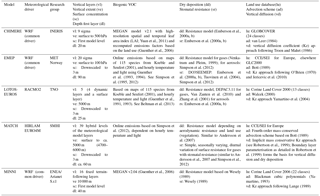
The CTMs were forced by regional numerical weather model simulations using boundary conditions from the ERA-Interim global reanalysis (Dee et al., 2011). Most of the CTMs used the same meteorological input data, with a few exceptions. Three of them (EMEP, CHIMERE and MINNI) used input meteorology from the Weather Research and Forecast Model (WRF) (Skamarock et al., 2008). LOTOS-EUROS and MATCH used the input meteorology produced by RACMO2 (van Meijgaard, 2012) and HIRLAM (Dahlgren et al., 2016), respectively. Unlike the rest of the regional weather models, RACMO2 used in the EDT exercise excluded nudging towards ERA-Interim, which might have some impact on the meteorological fields generated by RACMO2. A summary of the CTMs and the corresponding sources of meteorological input data with some of the main characteristics are given in Table 1. As with the observations, CTMs and their meteorological counterpart were interpolated to a common grid with horizontal resolution. The use of a coarser resolution could have an impact in some regions with a complex orography where airflow is usually controlled by mesoscale phenomena (e.g. sea breeze and mountain–valley winds) or in regions characterized by high-emission densities (Schaap et al., 2015; Gan et al., 2016). In such cases the use of a finer grid could be beneficial for capturing the variability of local processes.
A set of meteorological parameters was selected from the meteorological input data for the regression analyses. Similarly to the procedure with ERA-Interim, daily means are obtained from the available time steps every 3 hours in the case of WRF and RACMO2, and every 6 h for HIRLAM for the following variables: 10 m wind speed components, 2 m relative humidity and surface solar radiation. Maximum temperature is also approximated by the daily maximum of those time steps.
Summertime usually brings favourable conditions for high near-surface ozone concentrations, such as air stagnation due to high-pressure systems, warmer temperatures, higher UV radiation and lower cloud cover (Dawson et al., 2007). This study attempts to better understand how CTMs represent the meteorological sensitivities of ozone. To this aim, we use a multiple linear regression approach that can provide useful information on sensitivities in the distribution of ozone concentration as a whole (Porter et al., 2015).
Table 2List of the predictors used in the multiple linear regression analysis: meteorological parameters, lag of MDA8 O3 (24 h, previous day) and the seasonal cycle components.
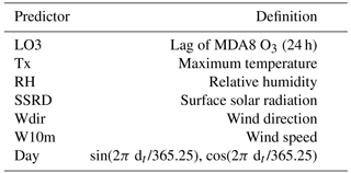
A total of five meteorological predictors (Table 2) are selected based on the existing literature that has shown their strong influence on ozone pollution (e.g. Bloomfield et al., 1996; Barrero et al., 2005; Camalier et al., 2007; Dawson et al., 2007; Andersson and Engardt, 2010; Rasmussen et al., 2012; Davis et al., 2011; Doherty et al., 2013; Otero et al., 2016). Moreover, it has been shown that the occurrence of air pollution episodes might increase when the pollution levels of the previous day are higher than normal (Ziomas et al., 1995). Then, apart from the meteorological predictors, we add the effect of the lag of ozone (MDA8 from the previous day) in order to examine the role of ozone persistence. Additionally, we include harmonic functions that capture the effect of seasonality as in Rust et al. (2009) and Otero et al. (2016), which is referred to as “day” in the MLRs (see Table 2).
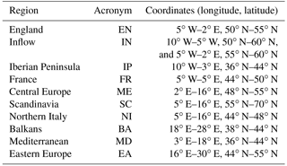
For this study, we divide the European domain into 10 regions: England (EN), Inflow (IN), Iberian Peninsula (IP), France (FR), central Europe (ME), Scandinavia (SC), northern Italy (NI), Mediterranean (MD), Balkans (BA) and eastern Europe (EA). These regions are based on those defined in the recent ETC/ACM technical paper (Colette et al., 2017b). For our study, we further subdivide the original Mediterranean region (MD) into a region covering the Balkans (BA) due to the strong influence of the ozone persistence on MDA8 O3 over this particular region as noted previously in Otero et al. (2016). Figure 1 shows the spatial coverage of each region and Table 3 lists their coordinates. As shown in Otero et al. (2016), the relative importance of predictors in the MLRs shows distinct seasonal patterns. Here, multiple linear regression models (MLRs, hereafter) are developed for each region for two seasons: springtime (April–May–June, AMJ) and summertime (July–August–September, JAS). These seasons differ from the meteorological definition but cover the period when surface ozone typically reaches its highest concentrations (i.e. April–September). Additionally, we analysed the impact of the seasons' definition by performing sensitivity tests using the meteorological seasons (i.e. March–May–April, MAM and June–July–August, JJA). As shown in Figs. S3 and S4, we found a stronger impact of some relevant key driving factors of ozone (e.g. temperature and relative humidity) when using the seasons defined above (AMJ and JAS) than when using the meteorological seasons. Therefore, we consider that our choice of 3-month periods that cover the whole ozone season is particularly useful for examining the impact of individual meteorological parameters when ozone levels are highest. Since the domains covered by observations and CTMs do not coincide exactly, we applied an observational mask to use the same number of grid cells for CTMs and observations. Data used to estimate parameters of the MLR were spatially averaged over each region. Thus, we compare MLRs developed separately for CTMs and observations for each region and season. The observational data set contains the gridded MDA8 O3 and the meteorology input from ERA-Interim, while the data set for the CTMs contains the MDA8 O3 from each one of them along with the corresponding meteorological input (LOTOS and RACMO2, CHIMERE and WRF, MATCH and HIRLAM) (see Table 1).
A MLR is built to describe the relationship between MDA8 O3 (predicant) and a set of covariates (or predictors) describing seasonality, ozone persistence and the influence of meteorological fields (Table 2). A data series yt, t=1, ...N (e.g. observations or CTM simulations) for a given region and season is conceived as a Gaussian random variable Yt with varying mean μt and homogeneous variance σ2. The mean μt is described as a linear function of the covariates, i.e.
with t indexing daily values and dt referring to the day of the year associated with the index t. β0 is a constant offset, βsin and βcos are the first-order coefficients of a Fourier series (e.g. Rust et al., 2009, 2013; Fischer et al., 2018), βlag describes the persistence with respect to the previous-day concentration yt−1 ; if t is the first day in the late summer season (JAS, 1 July), yt−1 is the concentration of 30 June. Further regression coefficients βk describe the linear relation to potential meteorological drivers (see Table 2). For covariates standardized to unit variance, the regression coefficients (β) are standardised coefficients giving the change in the predicant with the covariate in units of covariate standard deviation.
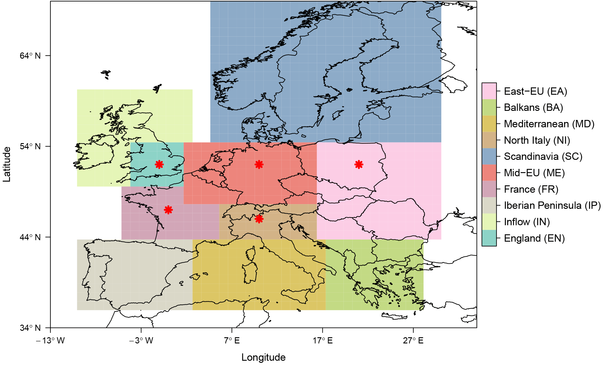
Figure 1Map of the regions considered in the study. Regions indicated with a black star refer to the internal regions in the text. The rest of regions refer to the external regions of the European domain.
Following the same strategy as used in Otero et al. (2016), the MLRs are developed through several common steps: (1) starting with the full set of potentially useful components in the predictor, a stepwise backward regression using the Akaike Information Criterion (AIC) as a selection criterion successively removes those components in the predictor, which contribute least to the model performance; and (2) a multi-collinearity index known as variance inflation factor (VIF, Maindonald and Braun, 2006) is used to detect multi-collinearity problems in the predictor (i.e. high correlations between two or more components in the predictor). Components with a VIF above 10 are left out of the predictor (Kutner et al., 2004).
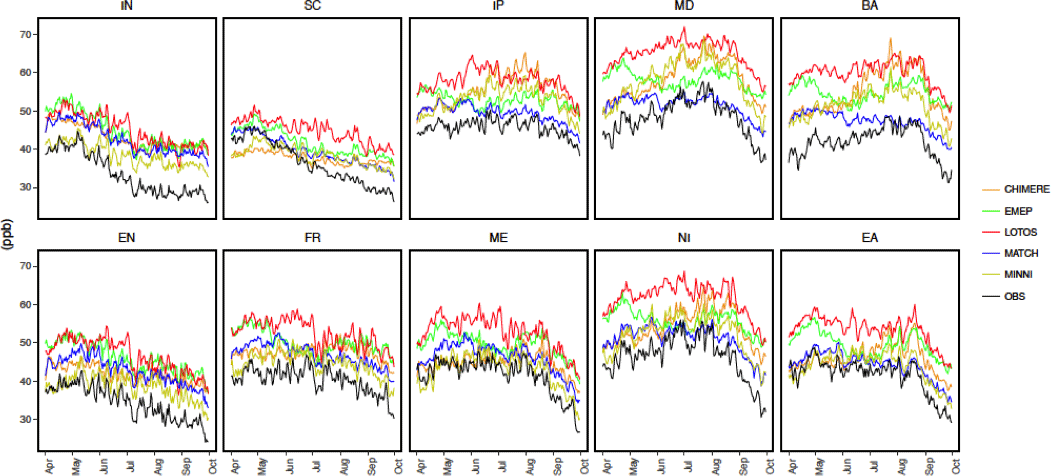
Figure 2Time series of daily averages of MDA8 O3 during the ozone season (April–September) for the period of study (2000–2010) at each subregion.
The statistical performance of each MLR (built separately from observations and CTMs) is assessed through the adjusted coefficient (R2) and the root mean square error (RMSE). The R2 estimates the fraction of total variability described by the MLR and the RMSE gives the average deviation between the model and observation obtained in the MLR. We also examine the relative importance of the individual components in the predictor. According to the method proposed by Lindeman et al. (1980), the relative importance of each predictor is estimated by its contribution to the R2 coefficient (Grömping, 2007). We assess the sensitivities of ozone to the predictors through the standardised coefficients obtained from the regression. These coefficients indicate the changes in the ozone response to the changes in the predictors, in terms of standard deviation. Thus, for every standard deviation unit increase (decrease) of a specific predictor, the predicant (MDA8 O3) will increase (decrease) the amount indicated by its coefficient in standard deviation units,. The use of standardised coefficients allows us to establish a direct comparison of the influence of individual predictors. The effect of seasonality introduced by the harmonic functions (namely, “day”; Table 2) is kept in the MLRs (Eq. 1) for its usefulness in improving the power of the regression analysis. However, further explanation about the effect of the predictors focuses on the rest of the variables.
4.1 CTM performance by region
We compare the seasonal cycle of observations and CTM results through the time series of daily averaged values of MDA8 O3 from observations and CTMs for the whole period (i.e. April–September, 2000–2010), spatially averaged over each region. Furthermore, correlation coefficients between both CTMs and observations at each region and season are used to quantify the CTM performance.
4.1.1 Seasonal cycle of MDA8 O3
We examine the ozone seasonal cycle represented by both the observational and modelled data sets. Figure 2 depicts daily averages during 2000–2010 of MDA8 O3 at each region for the CTMs and observations. In general, all CTMs are biased high compared with the observations. CTM results are visually closer to the observations in the north-western regions (i.e. IN, EN and FR), while the spread becomes larger over the southern and south-eastern regions (i.e. BA, NI, MD). The IN, EN and SC regions show the highest-observed concentrations in the starting months (AMJ), which are generally not well captured by most of the CTMs, which show a more flat timeline (e.g. LOTOS, MATCH, CHIMERE). For example, in the SC region, some of the CTMs underestimate the ozone concentrations in AMJ (i.e. CHIMERE and MINNI). The rest of the regions show the highest observed concentrations in JAS, which is generally overestimated by the CTMs. Models show discrepancies in the ozone seasonal cycle when compared to each other and when compared with observations. For example, we observed substantial differences in the southern regions, such as IP, MD and BA, where the models show a considerable spread. In those regions, the CTMs exhibit different behaviour when compared to each other. For instance, the EMEP model shows ozone peak concentrations in April, while CHIMERE and MINNI show a peak in July. Overall LOTOS shows a relatively constant positive bias in all regions, which is more evident in the MD and NI regions.
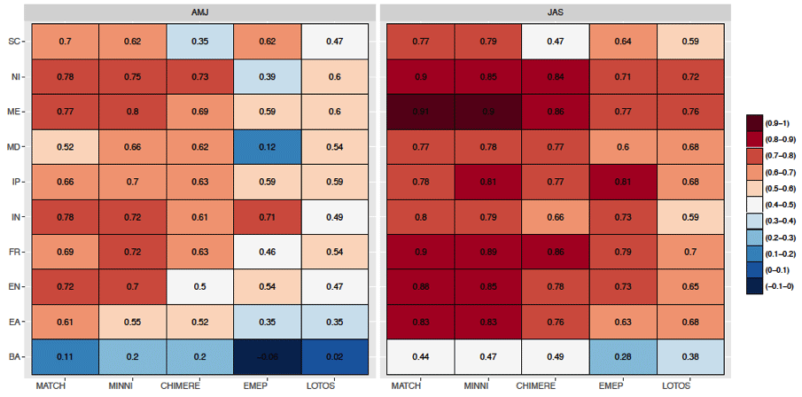
Figure 3Correlation coefficients between observed and modelled MDA8 O3 for spring (AMJ) and summer (JAS) for the period of study (2000–2010) at each region (rows) and model (columns, ordered by highest correlation values).
4.1.2 Correlation coefficients between modelled and observed time series
The correlation coefficients between the observed and modelled values of MDA8 O3 at each region and in each season are shown in Fig. 3. Overall, MDA8 O3 from the CTMs is better correlated with observations in JAS than in AMJ in the regions ME, NI, EA and EN. As expected from inspection of the average time series (Fig. 2), the lowest correlations between models and observations are found in BA, especially in AMJ for all models. In particular, EMEP is negatively correlated with observations over this region. As mentioned above, the larger discrepancies between CTMs and observations found over BA might be attributed to a low density of observation sites from which the interpolated data set is derived, resulting in a lower quality or higher uncertainties of such products (Schnell et al., 2014). The highest correlations in AMJ are obtained at the following regions, ME, FR, NI and EN, for most of the models, except for EMEP, for which the highest correlation with observations was found in IN and SC. In general, the models that are most closely correlated with observations are MATCH, MINNI and CHIMERE, while LOTOS shows the lowest correlations, which could be partially due to the use of a different set-up of the RACMO2 model, without nudging towards ERA-Interim (Sect. 2.2). These correlations reflect the patterns represented by the seasonal cycle described above.
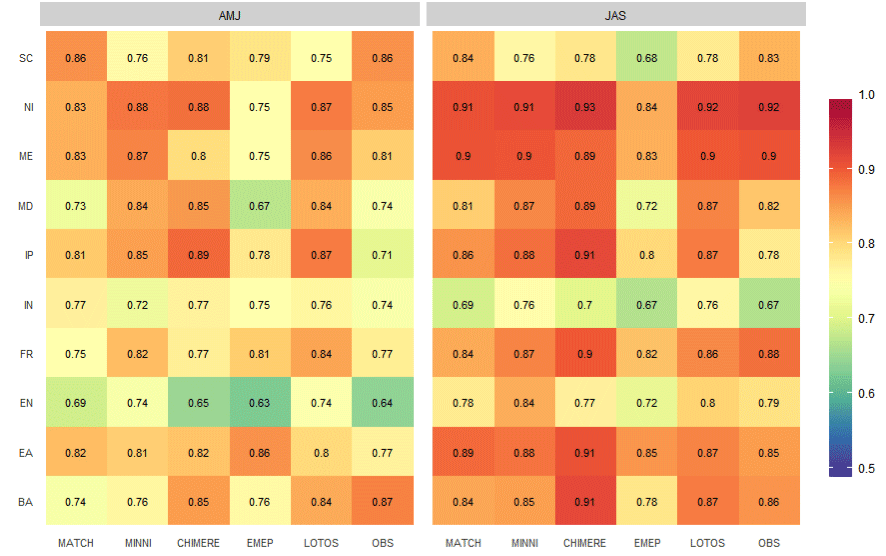
Figure 4Coefficients of determination (R2) for each CTM-based (ordered as in Fig. 3) and observation-based MLR in spring (AMJ) and summer (JAS).
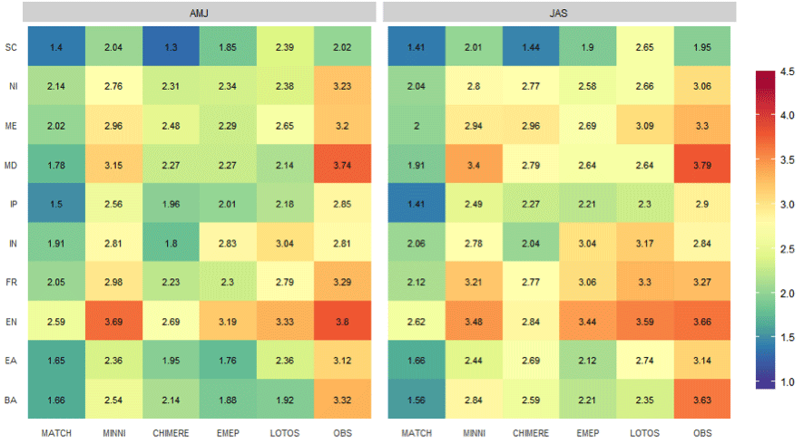
Figure 5Root mean square errors (RMSE) for each CTM-based (ordered as in Fig. 3) and observation-based MLR at each region, in spring (AMJ) and summer (JAS).
4.2 MLR performance
Figures 4 and 5 depict the statistical performance of each MLR in terms of R2 and RMSE (respectively) at the different regions for both seasons, AMJ and JAS. The R2 values indicate that all MLR models (based on both observations and CTMs) are able to explain more than 60 % of the MDA8 O3 variance in all regions. Overall, the MLRs show a stronger fit in JAS than in AMJ in most of the regions (Fig. 4). The MLRs appear to perform better in regions such as NI, ME, FR or EA, while the poorest statistical performance is found in IN and EN. The results obtained from the CTM-based MLRs show a similar performance to the observation-based MLRs in most of the regions. The lowest RMSE values for most of the MLR are found in SC ranging between 1 and 3 ppb, while EN shows the largest RMSE values. The MLRs from MATCH and CHIMERE show the lowest RMSE values (1–3 ppb), suggesting the best statistical fit from a predictive point of view.
Both R2 and RMSE metrics indicate that the statistical performance of MLRs for observations and CTMs show distinct variations between seasons and regions. Overall, better performances are found in JAS and in some regions (i.e. ME, NI, or FR) where MLRs are able to describe more than 80 % of the variance in CTMs and observations. This could be attributed to the major role of meteorology in summer influencing local photochemistry processes of ozone production, while in spring long-range transport plays a stronger role (Monks, 2000; Tarasova et al., 2007). As it includes the bias, the RMSE reveals more differences among the MLRs when compared to each other (e.g. larger errors for LOTOS when compared to MATCH or CHIMERE). However, it is interesting that in general all MLRs show a similar tendency when evaluating the statistical performance, which indicate that observation-based and CTM-based MLRs present a similar statistical performance for modelling MDA8 O3. The ability of the CTMs to reproduce the influence of meteorological drivers on MDA8 O3 is discussed in more detail below.
4.3 Effects of drivers on ozone concentrations
The analysis of the influence of the predictors in the MLRs reveals distinctive regional patterns in both observation-based and CTM-based MLRs. In agreement with Otero et al. (2016), here we also find that the regions geographically located towards the interior (including central, western and eastern regions) appear to be more sensitive to the meteorological predictors, especially in JAS. On the contrary, less of a meteorological contribution is found in the regions over the northernmost and southernmost part of the domain, implying that non-local processes (e.g. long-range transport) play a stronger role here. Considering such similarities, in the following, the regions EN, FR, ME, NI and EA are referred to as the internal regions, while the rest of the regions, IN, SC, IP, MD and BA, are referred to as the external regions (see Fig. 1).
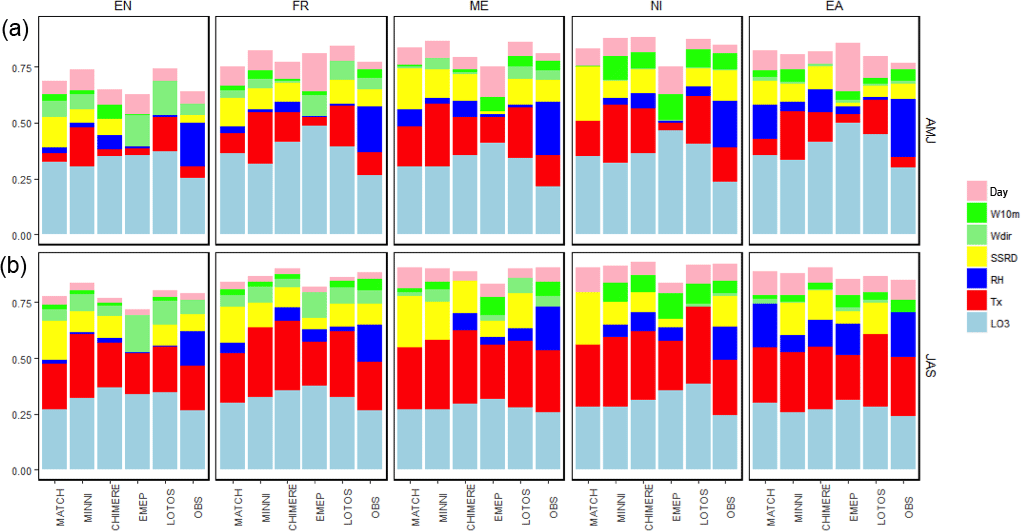
Figure 6Proportion of each predictor to the total explained variance for each CTM-based (ordered as in Fig. 3) and observation-based MLR in AMJ (a) and JAS (b) for the internal regions: England (EN), France (FR), central Europe (ME), northern Italy (NI) and eastern Europe (EA).
4.3.1 Relative importance
Figure 6 depicts the relative importance of the predictors for the observation-based and CTM-based MLRs in the internal regions (Fig. 1). Here, a larger meteorological influence (i.e. the predictors other than LO3 and day) can be seen in JAS compared to AMJ in all of these regions. In general, the dominant meteorological drivers from the observation-based MLRs in these internal regions are RH and Tx. The contribution of RH is evident in AMJ (e.g. ME, or EA), while Tx is clearly dominant in JAS. SSRD is also a key driver of MDA8 O3, and generally, the wind factors (W10m and Wdir) appear to have a minor contribution.
Despite the CTM-based MLRs being able to capture the meteorological predictors, we observe discrepancies among the internal regions when compared to the observation-based MLR. The inter-model differences in terms of the relative importance of predictors are greater in AMJ than in JAS. For instance, the contribution of the LO3 is overestimated by CTMs. Substantial differences are found in the influence of RH when comparing the observation-based and the CTM-based models. The CTMs do not capture the relative importance of the RH well, especially in AMJ. In general, the CTMs driven by WRF meteorology show a slightly larger contribution of RH in most cases, although we notice that there are also some differences among the models that share the same meteorology. CTMs do capture the relative importance of Tx in all regions, but overall they overestimate it, as they also show for SSRD. Here, we find discrepancies when comparing the contribution of predictors in the statistical models from CTMs driven by the same meteorology (e.g. EMEP when compared to CHIMERE and MINNI). Such differences among the models using the same meteorology point out that the model set-up (e.g. number of vertical levels, depth of first layer) and model parameterizations (e.g. chemistry-physical processes) have a larger influence in the model performance than the meteorological processes.
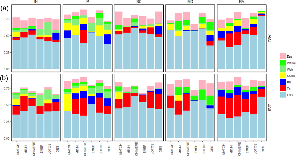
Figure 7Proportion of each predictor to the total explained variance for each CTM-based (ordered as in Fig. 3) and observation-based MLR in AMJ (a) and JAS (b) for the external regions: Inflow (IN), Iberian Peninsula (IP), Scandinavia (SC), Mediterranean (MD) and Balkans (BA).
Figure 7 presents the relative importance of individual predictors in the MLRs developed at the external regions (Fig. 1) for both seasons. The observation-based MLRs show that the main driving factor is LO3 in AMJ, while the effect of meteorological drivers becomes stronger in JAS. RH presents a larger contribution in some regions (e.g. IN, IP or SC) in AMJ and Tx in JAS (e.g. IN, IP, SC and BA). The contribution of wind components, Wdir and W10m, is mainly reflected in both seasons in the western regions (i.e. IN and IP) and in MD, respectively.
Overall, all CTMs show this tendency, although there are substantial differences when comparing the individual drivers' contributions in the observation-based and CTM-based MLRs, particularly in AMJ (Fig. 7). CTMs do not capture the contribution of LO3 reflected by the observation-based MLRs. As in the previous analysis (Sect. 4.1), the largest discrepancies are found in BA. In this region, the observation-based MLR shows that most of the variability of ozone would be explained by LO3, while the CTM-based MLRs underestimate the contribution of LO3 and overestimate the meteorological contribution of Tx, SSRD and RH (e.g. LOTOS, CHIMERE and MINNI). The contribution of RH is, again, underestimated by the CTMs in most of the regions (except in BA). On the contrary, the relative importance of SSRD is overestimated in some regions (e.g. IP, IN or MD) and Tx (IN, SC), in particular for the CTMs driven by WRF. Overall, CTMs show the observed contribution of W10m and Wdir in both seasons, although with some inconsistences among the regions and CTMs.
Our results indicate that the relative importance of meteorological factors is stronger in the internal regions (Fig. 6) than in the external regions (Fig. 7), which could be partially attributed to a larger variability of most of the meteorological fields in internal regions (Fig. S5). The external regions are also more likely to be influenced by the lateral boundary conditions applied by each CTM. In addition, in some external regions (e.g. IP or MD), as mentioned in Sect. 2, the use of a coarser grid in some regions might be insufficient to capture mesoscale processes, such as land–sea breezes, which also control MDA8 O3 concentrations (Millán et al., 2002). Moreover, we observe that meteorology becomes more important in summer, when local photochemistry processes are dominant. In general, CTMs show this tendency but limitations in reproducing the effect of some meteorological drivers are found. Specifically, while CTMs tend to overestimate the contribution of Tx and SSRD, they underestimate the relative importance of RH, which is also reflected in the correlation coefficients between predicant and the predictors (Figs. S6, S7).
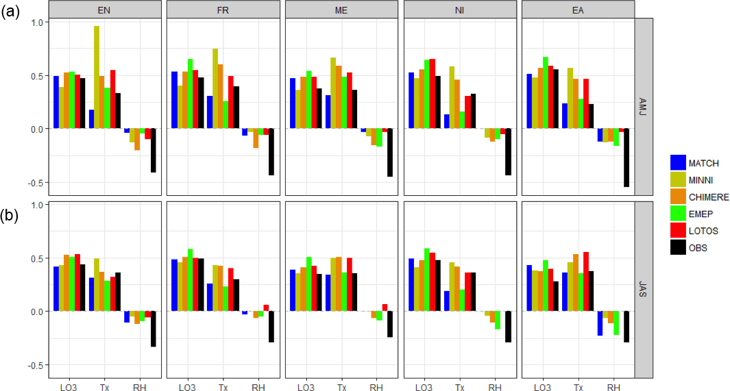
Figure 8Standardised coefficient values of the key driving factors (LO3, Tx and RH) for each CTM-based (ordered as in Fig. 3) and observation-based MLR in AMJ (a) and JAS (b) and for the internal regions: England (EN), France (FR), central Europe (ME), northern Italy (NI) and eastern Europe (EA).
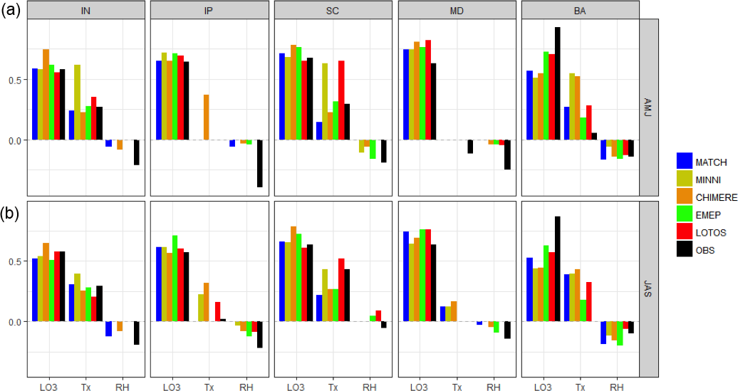
Figure 9Standardised coefficients values of the main key-driving factors (LO3, Tx and RH) for each CTM-based (ordered as in Fig. 3) and observation-based MLR in AMJ (a) and JAS (b) and for the external regions: Inflow (IN), Iberian Peninsula (IP), Scandinavia (SC), Mediterranean (MD) and Balkans (BA).
4.3.2 Sensitivity of ozone to the drivers
We assess the sensitivities of MDA8 O3 to the drivers through their standardised coefficients obtained in the MLR (Sect. 3). These coefficients provide further information about the changes in MDA8 O3 due to the effect of each driver. Figures 8 and 9 depict the values of the main driving factors obtained in the MLR for the internal and the external regions (respectively): LO3, Tx and RH. Similarly to those patterns described by the relative importance of drivers, we observe that the ozone response to LO3 is stronger in AMJ than in JAS: the corresponding standardised coefficients are always positive and generally higher in AMJ. The observed sensitivities to LO3 are smaller in the internal regions (Fig. 8), being particularly dominant in the external regions (Fig. 9). Overall, most of the CTMs reflect a similar tendency. However, there are evident differences between observations and CTMs when comparing the values of the standardised coefficients, specifically in some regions such as BA or MD. When comparing the ozone responses of the CTMs to LO3, we observe that in most of the regions MATCH and MINNI show values closest to observations, which is consistent with the results described at the beginning of this Sect. 4.1.2.
Correlations between MDA8 O3 and Tx are strong, especially in the internal regions in JAS (Fig. S6). Overall, we show that the CTMs appear to capture the observed effect of Tx better in JAS than in AMJ in most of the regions. The highest sensitivities to Tx are found in internal regions such as ME, NI, FR and EN, which is also shown in the CTMs (Fig. 8). However, we see that most of the CTMs tend to overestimate the effect of Tx and distinct sensitivities to Tx are also found for those models that share the same meteorology (i.e. CHIMERE, EMEP and MINNI). In particular, the MINNI and CHIMERE models show higher Tx sensitivities when compared to the rest of the CTMs. While the MINNI model presents the highest sensitivities to Tx in spring, especially in EN and FR, EMEP shows smaller values and it underestimates the correlations between Tx and MDA8 O3 (Figs. S6, S7).
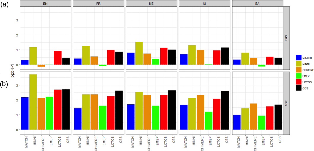
Figure 10Slopes (mO3−T; ppbK−1) obtained from a simple linear regression to estimate the relationship of ozone–temperature for each CTM-based (ordered as in Fig. 3) and observation-based MLR in AMJ (a) and JAS (b) and for the internal regions: England (EN), France (FR), central Europe (ME), northern Italy (NI) and eastern Europe (EA).

Figure 11Slopes (mO3−T; ppbK−1) obtained from a simple linear regression to estimate the relationship of ozone–temperature for each CTM-based (ordered as in Fig. 3) and observation-based MLR in AMJ (a) and JAS (b) and for the external regions: Inflow (IN), Iberian Peninsula (IP), Scandinavia (SC), Mediterranean (MD) and Balkans (BA).
The slope of the ozone–temperature relationship (mO3−T) has been used in several studies to assess the ozone climate penalty (e.g. Bloomer et al., 2009; Steiner et al., 2006; Rasmussen et al., 2012; Brown-Steiner et al., 2015) in the context of future air quality. Thus, we additionally analyse the ozone–temperature relationship in order to provide insight into the ability of CTMs to reproduce the observed mO3−T. Similarly to previous work (Brown-Steiner et al., 2015), the slopes are obtained from a simple linear regression using only Tx (without the influence from other predictors) and they are used to quantify this relationship in both seasons, AMJ and JAS.
Figures 10 and 11 illustrate the mO3−T for the internal and external regions respectively. The observed mO3−T is larger in JAS than in AMJ. In AMJ, it ranges between −0.45 and 1.15 ppbK−1 with the largest values found in ME, NI and MD. In JAS, the observed climate penalty is of the order of 1–2.7 ppbK−1 with the largest values in EN, FR, ME, NI and MD. CTMs show a better agreement with observations in JAS than in AMJ. CTMs tend to overestimate the climate penalty in AMJ in most of the regions, with some exceptions, such as EMEP and MATCH, which systematically underestimate the slopes. Also, CTMs are generally better at simulating the observed mO3−T in the internal regions compared to the mO3−T in the external regions, where in general CTMs appear to overestimate the climate penalty in both seasons. Using this metric, we identify some regions that are particularly sensitive to temperature, with larger values of mO3−T (e.g. EN, ME, FR, NI or MD). Through a multi-model assessment, Colette et al. (2015) showed a significant summertime climate penalty in southern, western and central European regions (e.g. EA, IP, FR, ME or MD) in the majority of the future climate scenarios used. Our study shows that most of the CTMs confirm the observed climate penalty in JAS in these regions in the near present, although we found that most of the CTMs overestimate the climate penalty in AMJ, especially in the external regions.
We see a stronger effect of RH in AMJ than in JAS in the observations, with the greatest impact in the internal regions (e.g. EA, ME, NI, FR and EN), which is not well represented by the CTMs (Figs. 8 and 9). As mentioned, CTMs underestimate the strength of the correlations between ozone and relative humidity (Figs. S6, S7). This general lack of sensitivity to RH could also partially explain the tendency for all CTMs to show a high bias in simulated ozone compared with observations (Fig. 2). Among the possible reasons for this inconsistency, we hypothesize that it can be related to the fact that ozone removal processes can be associated with higher relative humidity levels during thunderstorm activity on hot moist days, which might not be well captured by CTMs. As previous studies pointed out (e.g. Andersson and Engardt, 2010), the impacts of ozone dry deposition suggest that it may also play a role in explaining the problems that CTMs show to reproduce the observed ozone-relative humidity relationship. With a simple modelling approach, Kavassalis and Murphy (2017) found that the relationship between ozone and relative humidity was better captured by the inclusion of the vapour pressure deficit-dependent dry deposition, pointing out the relevance of detailed dry-deposition schemes in the CTMs.
High SSRD levels favour photochemical ozone formation and are usually positively correlated to ozone. In this case, CTMs also present some limitations in capturing this effect and they overestimated the sensitivities of ozone to SSRD (Figs. S8, S9). For example, the observations show a lower and surprisingly negative effect of SSRD. Although the correlations between SSRD and ozone are positive (see Figs. S6, S7), the presence of other predictors in the regression may reverse the sign of the estimated coefficient. The CTMs show a stronger sensitivity of ozone to SSRD and they overestimate its influence on surface ozone. Similarly, the sensitivities to Wdir and W10m are also overestimated by the CTMs, especially in AMJ (Figs. S8, S9).
Our analysis suggests that CTMs present more limitations to reproduce the influence of meteorological drivers to MDA8 O3 concentrations in the external regions than in the internal regions, particularly in AMJ. Moreover, we find the largest discrepancies in BA, where models show the poorest seasonal performance and correlation coefficients (Figs. 2 and 3, respectively), probably due a low quality of the observational data set.
Furthermore, LO3 is the main driver over most of the external regions and explains a large proportion of the total variability of MDA8 O3, while meteorological factors have a smaller influence. Lemaire et al. (2016) found a very low performance (based on R2) over the British Isles, Scandinavia and the Mediterranean using a different statistical approach that only included two meteorological drivers. They attributed this low skill to the large influence over those regions of long-range transport of air pollution (Lemaire et al., 2016). Our results confirm the small influence of the meteorological drivers over those regions and the strong influence of the ozone persistence. Moreover, in the case of the external regions of northern Europe, it could also be explained due to the dominance of transport processes such as the stratospheric–tropospheric exchange or long-range transport from the European continent, rather than local meteorology, particularly in AMJ (Monks, 2000; Tang et al., 2009; Andersson et al., 2009).
Previous work suggested that local sources of NOx and biogenic VOC (ozone precursors) are important factors of summertime ozone pollution in the Mediterranean basin (Richards et al., 2013). Moreover, some studies suggested that the local vertical recirculation and accumulation of pollutants play an important role in ozone pollution episodes in this region: during the night-time the air masses are held offshore by a land–sea breeze, creating reservoirs of pollutants that are brought back the following day (Millán et al., 20002; Jiménez et al., 2006; Querol et al., 2017). All of these factors (e.g. local emissions as well as local and large-scale processes) control the ozone variability, which might explain the smaller influence of local meteorological factors shown in this study over the Mediterranean basin when compared to meteorological influence in the internal regions. Thus, we may hypothesize that the strong impact of LO3 observed in the external regions over southern Europe (i.e. IP, MD, BA) could be partially due to the role of vertical accumulation and recirculation of air masses along the Mediterranean coasts as a result of the mesoscale phenomena, which is enhanced by the complex terrains that surround the basin. Another important factor for the strong impact of LO3 observed is the slow dry deposition of ozone on water that would favour the ozone persistence in southern Europe.
Overall we conclude that CTMs capture the effect of meteorological drivers better in the internal regions (EN, FR, ME, NI and EA), where the influence of local meteorological conditions is stronger. The major effect of meteorological parameters found in the internal European regions might also be attributed to the fact that overall the variability of meteorological conditions is larger in those regions (Fig. S5). We also find differences among the CTMs driven by the same meteorology. As mentioned in the introduction, Bessagnet et al. (2016) suggested that the spread in the model results could be partly explained by the differences in the vertical turbulent mixing in the planetary boundary layer, which are differently diagnosed in each of the CTMs. Our results also indicate that, even though models share the same meteorology (considering the prescribed requirements defined by the EDT exercise), they show discrepancies when compared to each other, which could be attributed to other sources of uncertainties (such as physical and chemical internal processes in the CTMs). The NMVOC and NOx emissions from the biosphere are critical in the ozone formation. Since biogenic emissions were not specifically prescribed and have a strong dependence on temperature and solar radiation, discrepancies in the CTMs performances, (e.g. different sensitivities to Tx) might be expected. Furthermore, we notice that the CTMs do not consistently reproduce the regional ozone–temperature relationship, which is a key factor when assessing the impacts of climate change on future air quality.
The present study evaluates the capabilities of a set of chemical transport models (CTMs) to capture the observed meteorological sensitivities of daily maximum 8 h average ozone (MDA8 O3) over Europe. Our study reveals systematic differences between the CTMs in reproducing the seasonal cycle when compared to observations. In general, CTMs tend to overestimate the MDA8 O3 in most of the regions. In the western and northern regions (i.e. Inflow, England and Scandinavia), some models did not capture the high ozone levels in spring (e.g. CHIMERE and MINNI), while in some southern regions (e.g. Iberian Peninsula, Mediterranean and Balkans) they overestimated the ozone levels in summer (e.g. LOTOS, CHIMERE). Of the CTMs, MATCH and MINNI were the most successful in capturing the observed seasonal cycle of ozone in most regions. All CTMs revealed limitations in reproducing the variability of ozone over the Balkans region, with a general overestimation of the ozone concentrations that was considerably larger during the warmer months (July, August). As reflected in the results, a limitation of the interpolated observational product used here is that in some regions (e.g. southern Europe) it has a lower quality due to a reduced number of stations (Sect. 2.1).
The MLRs performed similarly for most of the CTMs and observations, describing more than 60 % of the total variance of MDA8 O3. Overall, the MLRs perform better in JAS than in AMJ, and the highest percentages of described variance were found in central Europe and northern Italy. This could be attributed to local photochemical processes being more important in JAS and is consistent with a relatively stronger influence of long-range transport in AMJ.
The effects of predictors revealed spatial and seasonal patterns, in terms of their relative importance in the MLRs. Particularly, we noticed a larger local meteorological influence in the regions located towards the interior of Europe, here termed the internal regions (i.e. England, France, central Europe, northern Italy and eastern Europe). A minor local meteorological contribution was found in the remaining regions, referred to as the external regions (i.e. Inflow, Iberian Peninsula, Scandinavia, Mediterranean and Balkans). The CTMs are in better agreement with the observations in the internal regions than in the external regions, where they were not as successful in reproducing the effects of the ozone drivers. Overall, different behaviour in the MLRs developed in the external regions could be attributed to (i) a larger influence of dynamical processes rather than local meteorological processes (e.g. long-range transport in the northern regions), (ii) a stronger impact of the boundary conditions and (iii) the use of a coarser grid that might be insufficient to capture mesoscale processes that also influence MDA8 O3 (e.g. sea–land breezes in the southern regions).
We found substantial differences in the sensitivities of MDA8 O3 to the different meteorological factors among the CTMs, even when they used the same meteorology. As Bessagnet et al. (2016) point out, the differences among CTMs could be partly attributed to some other diagnosed model variables (e.g. vertical turbulent mixing and boundary layer height, as well as vertical model resolution). To assess the effect of such potential sources of uncertainties, further investigations would be required. Moreover, variations in the sensitivity of ozone to meteorological parameters could depend on differences in the chemical and photolysis mechanisms and the implementation of various physics schemes, all of which differ between the CTMs (see Colette et al., 2017a). Specifically, the discrepancies found in the sensitivities of MDA8 O3 to maximum temperature might also be attributed to biogenic emissions not prescribed in the models. This was particularly reflected in the analysis of the slopes' ozone–temperature relationship (mO3−T) to assess the climate penalty, which differed between CTMs and regions when compared to the observations in both seasons. Most of the CTMs confirm the observed climate penalty in JAS but with larger discrepancies in the external regions than in the internal regions. Furthermore, CTMs tend to overestimate the climate penalty in AMJ (particularly in the external regions).
Our results have shown discrepancies in the observed and simulated ozone sensitivities to relevant meteorological parameters for ozone formation and removal processes. In particular, we found that CTMs tend to overestimate the influence of maximum temperature and surface solar radiation in most of the regions, both of which are strongly associated with ozone production. None of the CTMs captured the strength of the observed relationship between ozone and relative humidity appropriately, underestimating the effect of relative humidity, a key factor in the ozone removal processes. We speculate that ozone dry-deposition schemes used by the CTMs in this study may not adequately represent the relationship between humidity and stomatal conductance, thus underestimating the ozone sink due to stomatal uptake. Further sensitivity analyses would be recommended for testing the impact of the current dry-deposition schemes in the CTMs.
The data are available upon request from the corresponding author.
The supplement related to this article is available online at: https://doi.org/10.5194/acp-18-12269-2018-supplement.
NO prepared the data set provided by the EURODELTA working group, performed the analysis and wrote the paper. TB, JS helped to guide the data analysis, and HWR provided statistical support and help to interpret the results. The rest of the co-authors contributed in scientific discussions and the whole team helped to prepare the final version of the paper.
The authors declare that they have no conflict of interest.
This work was hosted by IASS Potsdam, with financial support provided by the
Federal Ministry of Education and Research of Germany (BMBF) and the Ministry
for Science, Research and Culture of the State of Brandenburg (MWFK). The
authors acknowledge Jordan L. Schnell for providing the interpolated data set
of MDA 8 O3. Modelling data used in the present analysis were produced in the
framework of the EURODELTA-Trends project initiated by the Task Force on
Measurement and Modelling of the Convention on Long Range Transboundary Air
Pollution. EURODELTA-Trends is coordinated by INERIS and involves modelling
teams from BSC, CEREA, CIEMAT, ENEA, IASS, JRC, MET Norway, TNO and SMHI. The
views expressed in this study are those of the authors and do not
necessarily represent the views of EURODELTA-Trends modelling teams. The
MATCH participation was partly funded by the Swedish Environmental Protection
Agency through the research programme Swedish Clean Air and Climate (SCAC)
and NordForsk through the research programme Nordic WelfAir (grant no.
75007). Jana Sillmann is supported by the Research Council of Norway through
the CIXPAG project (grant no. 244551).
Edited
by: Jørgen Brandt
Reviewed by: four anonymous referees
Andersson, C. and Engardt, M.: European ozone in a future climate: Importance of changes in dry deposition and isoprene emissions, J. Geophys. Res.-Atmos., 115, D02303, https://doi.org/10.1029/2008jd011690, 2010.
Andersson, C., Langner, J., and Bergström, R.: Interannual variation and trends in air pollution over Europe due to climate variability during 1958–2001 simulated with a regional CTM coupled to the ERA-40 reanalysis, Tellus B, 59, 77–98, 2007.
Andersson, C., Bergström, R., and Johansson, C.: Population exposure and mortality due to regional background PM in Europe–Long-term simulations of source region and shipping contributions, Atmos. Environ., 43, 3614–3620, https://doi.org/10.1016/j.atmosenv.2009.03.040, 2009.
Barrero, M. A., Grimalt, J. O., and Canton, L.: Prediction of daily ozone concentration maxima in the urban atmosphere, Chemometr. Intell. Lab. Syst., 80, 67–76, 2005.
Beltman, J. B., Hendriks, C., Tum, M., and Schaap, M.: The impact of large scale biomass production on ozone air pollution in Europe, Atmos. Environ., 71, 352–363, 2013.
Bessagnet, B., Pirovano, G., Mircea, M., Cuvelier, C., Aulinger, A., Calori, G., Ciarelli, G., Manders, A., Stern, R., Tsyro, S., García Vivanco, M., Thunis, P., Pay, M.-T., Colette, A., Couvidat, F., Meleux, F., Rouïl, L., Ung, A., Aksoyoglu, S., Baldasano, J. M., Bieser, J., Briganti, G., Cappelletti, A., D'Isidoro, M., Fi- nardi, S., Kranenburg, R., Silibello, C., Carnevale, C., Aas, W., Dupont, J.-C., Fagerli, H., Gonzalez, L., Menut, L., Prévôt, A. S. H., Roberts, P., and White, L.: Presentation of the EURODELTA III intercomparison exercise – evaluation of the chemistry transport models' performance on criteria pollutants and joint analysis with meteorology, Atmos. Chem. Phys., 16, 12667–12701, https://doi.org/10.5194/acp-16-12667-2016, 2016.
Bloomer, B. J., Stehr, J. W., Piety, C. A., Salawitch, R. J., and Dickerson, R. R.: Observed relationships of ozone air pollution with temperature and emissions, Geophys. Res. Lett., 36, L09803, https://doi.org/10.1029/2009gl037308, 2009.
Bloomfield, P. J., Royle, J. A., Steinberg, L. J., and Yang, Q.: Accounting for meteorological effects in measuring urban ozone levels and trends, Atmos. Environ., 30, 3067–3077, 1996.
Bott, A.: A Positive Definite Advection Scheme Obtained by Nonlinear Renormalization of the Advective Fluxes, Mon. Weather Rev., 117, 1006–1015, 1989.
Brown-Steiner, B., Hess, P. G., and Lin, M. Y.: On the capabilities and limitations of GCCM simulations of summertime regional air quality: A diagnostic analysis of ozone and temperature simulations in the US using CESM CAM-Chem, Atmos. Environ., 101, 134–148, https://doi.org/10.1016/j.atmosenv.2014.11.001, 2015.
Brunner, D., Jorba, O., Savage, N., Eder, B., Makar, P., Giordano, L., Badia, A., Balzarini, A., Baro, R., Bianconi, R., Chemel, C., Forkel, R., Jimenez-Guerrero, P., Hirtl, M., Hodzic, A., Honzak, L., Im, U., Knote, C., Kuenen, J. J. P., Makar, P. A., MandersGroot, A., Neal, L., Perez, J. L., Pirovano, G., San Jose, R., Savage, N., Schroder, W., Sokhi, R. S., Syrakov, D., Torian, A., Werhahn, K., Wolke, R., van Meijgaard, E., Yahya, K., Zabkar, R., Zhang, Y., Zhang, J., Hogrefe, C., and Galmarini, S.: Comparative analysis of meteorological performance of coupled chemistry-meteorology models in the context of AQMEII phase 2, Atmos. Environ., 115, 470–498, 2015.
Camalier, L., Cox, W., and Dolwick, P.: The effects of meteorology on ozone in urban areas and their use in assessing ozone trends, Atmos. Environ., 41, 7127–7137, 2007.
Carro-Calvo, L., Ordóñez, C., García-Herrera, R., and Schnell, J. L.: Spatial clustering and meteorological drivers of summer ozone in Europe, Atmos. Environ., 167, 496–510, https://doi.org/10.1016/j.atmosenv.2017.08.050, 2017.
Colette, A., Andersson, C., Baklanov, A., Bessagnet, B., Brandt, J., Christensen, J., Doherty, R., Engardt, M., Geels, C., Giannakopoulos, C., Hedegaard, G., Katragkou, E., Langner, J., Lei, H., Manders, A., Melas, D., Meleux, F., Rouil, L., Sofiev, M., Soares, J., Stevenson, D., Tombrou-Tzella, M., Varotsos, K., and Young, P.: Is the ozone climate penalty robust in Europe?, Environ. Res. Lett., 10, 084015, https://doi.org/10.1088/1748-9326/10/8/084015, 2015.
Colette, A., Andersson, C., Manders, A., Mar, K., Mircea, M., Pay, M.-T., Raffort, V., Tsyro, S., Cuvelier, C., Adani, M., Bessagnet, B., Bergström, R., Briganti, G., Butler, T., Cappelletti, A., Couvidat, F., D'Isidoro, M., Doumbia, T., Fagerli, H., Granier, C., Heyes, C., Klimont, Z., Ojha, N., Otero, N., Schaap, M., Sindelarova, K., Stegehuis, A. I., Roustan, Y., Vautard, R., van Meijgaard, E., Vivanco, M. G., and Wind, P.: EURODELTA-Trends, a multi-model experiment of air quality hindcast in Europe over 1990–2010, Geosci. Model Dev., 10, 3255–3276, https://doi.org/10.5194/gmd-10-3255-2017, 2017a.
Colette, A., Solberg, S., Beauchamp, M., Bessagnet, B., Malherbe, L., and Guerreiro, C.: Long term air quality trends in Europe: Contribution of meteorological variability, natural factors and emissions, ETC/ACM, Bilthoven, 2017b.
Dahlgren, P., Landelius, T., Kållberg, P., and Gollvik, S.: A high-resolution regional reanalysis for Europe. Part 1: Three-dimensional reanalysis with the regional HIgh-Resolution Limited-Area Model (HIRLAM), Q. J. Roy. Meteorol. Soc., 142, 2119–2131, https://doi.org/10.1002/qj.2807, 2016.
Davis, J., Cox, W., Reff, A., and Dolwick, P.: A comparison of Cmaq-based and observation-based statistical models relating ozone to meteorological parameters, Atmos. Environ., 45, 3481e3487, https://doi.org/10.1016/J.Atmosenv.2010.12.060, 2011.
Dawson, J. P., Adams, P. J., and Pandis, S. N.: Sensitivity of ozone to summertime climate in the Eastern USA: a modeling case study, Atmos. Environ., 41, 1494–1511, 2007.
Dee, D. P., Uppala, S. M., Simmons, A. J., Berrisford, P., Poli, P., Kobayashi, S., Andrae, U., Balmaseda, M. A., Balsamo, G., Bauer, P., Bechtold, P., Beljaars, A. C. M., van de Berg, L., Bidlot, J., Bormann, N., Delsol, C., Dragani, R., Fuentes, M., Geer, A. J., Haimberger, L., Healy, S. B., Hersbach, H., Hólm, E. V., Isaksen, L., Kållberg, P., Köhler, M., Matricardi, M., McNally, A. P., Monge-Sanz, B. M., Morcrette, J. J., Park, B. K., Peubey, C., de Rosnay, P., Tavolato, C., Thépaut, J. N., and Vitart, F.: The ERA-Interim reanalysis: configuration and performance of the data assimilation system, Q. J. Roy. Meteorol. Soc., 137, 553–597, 2011.
Doherty, R. M., Wild, O., Shindell, D. T., Zeng, G., MacKenzie, I. A., Collins, W. J., Fiore, A. M., Stevenson, D. S., Dentener, F. J., Schultz, M. G., Hess, P., Derwent, R. G., and Keating, T. J.: Impacts of climate change on surface ozone and intercontinental ozone pollution: a multi- model study, J. Geophys. Res.-Atmos., 118, 3744–3763, https://doi.org/10.1002/jgrd.50266, 2013.
Dueñas, C., Fernandez, M. C., Canete, S., Carretero, J., and Liger, E.: Assessment of ozone variations and meteorological effects in an urban area in the Mediterranean Coast, Sci. Total Environ., 299, 97–113, 2002.
Emberson, L. D., Ashmore, M. R., Simpson, D., Tuovinen, J.-P., and Cambridge, H. M.: Towards a model of ozone deposition and stomatal uptake over Europe, Norwegian Meteorological Institute, Oslo, Norway, 57, 2000a.
Emberson, L. D., Ashmore, M. R., Simpson, D., Tuovinen, J.-P., and Cambridge, H. M.: Modelling stomatal ozone flux across Europe, Water Air Soil Pollut., 109, 403–413, 2000b.
Fiore, A. M., Dentener, F. J., Wild, O., Cuvelier, C., Schultz, M. G., Hess, P., Textor, C., Schulz, M., Doherty, R. M., Horowitz, L. W., MacKenzie, I. A., Sanderson, M. G., Shindell, D. T., Stevenson, D. S., Szopa, S., Van Dingenen, R., Zeng, G., Atherton, C., Bergmann, D., Bey, I., Carmichael, G., Collins, W. J., Duncan, B. N., Faluvegi, G., Folberth, G., Gauss, M., Gong, S., Hauglustaine, D., Holloway, T., Isaksen, I. S. A., Jacob, D. J., Jonson, J. E., Kaminski, J. W., Keating, T. J., Lupu, A., Marmer, E., Montanaro, V., Park, R. J., Pitari, G., Pringle, K. J., Pyle, J. A., Schroeder, S., Vivanco, M. G., Wind, P., Wojcik, G., Wu, S., and Zuber, A.: Multimodel estimates of intercontinental source-receptor relationships for ozone pollution, J. Geophys. Res.-Atmos., 114, D04301, https://doi.org/10.1029/2008jd010816, 2009.
Fischer M., Rust H. W., and Ulbrich U.: Seasonal Cycle in German Daily Precipitation Extremes, Meteorologische Z., 27, 3–13, https://doi.org/10.1127/metz/2017/0845, 2018.
Fix, M. J., Cooley, D., Hodzic, A., Gilleland, E., Russell, B. T., Porter, W. C., and Pfister, G. G.: Observed and predicted sensitivities of extreme surface ozone to meteorological drivers in three US cities, Atmos. Environ., 176, 292–300, https://doi.org/10.1016/j.atmosenv.2017.12.036, 2018
Gan, C., Hogrefe, C., Mathur, R., Pleim, J., Xing, J., Wong, D., Gilliam, R., Pouliot, G., and Wei, C.: Assessment of the effects of horizontal grid resolution on long-term air quality trends using coupled WRF-CMAQ simulations, Atmos. Environ., 132, 207–216, 1352–2310, https://doi.org/10.1016/j.atmosenv.2016.02.036, 2016.
Grömping, U.: Estimators of relative importance in linear regression based on variance decomposition, Am. Stat., 61, 139–147, 2007.
Guenther, A. B., Monson, R. K., and Fall, R.: Isoprene and monoterpene emission rate variability: Observations with eucalyptus and emission rate algorithm development, J. Geophys. Res.-Atmos., 96, 10799–10808, 1991.
Guenther, A., Zimmerman, P., Harley, P., Monson, R., and Fall, R.: Isoprene and monoterpene rate variability: model evaluations and sensitivity analyses, J. Geophys. Res., 98, 12609–12617, 1993.
Guenther, A., Zimmerman, P., and Wildermuth, M.: Natural volatile organic compound emission rate estimates for US woodland landscapes, Atmos. Environ., 28, 1197–1210, 1994.
Guenther, A., Karl, T., Harley, P., Wiedinmyer, C., Palmer, P. I., and Geron, C.: Estimates of global terrestrial isoprene emissions using MEGAN (Model of Emissions of Gases and Aerosols from Nature), Atmos. Chem. Phys., 6, 3181–3210, doi10.5194/acp-6-3181-2006, 2006.
Hedegaard, G. B., Christensen, J. H., and Brandt, J.: The relative importance of impacts from climate change vs. emissions change on air pollution levels in the 21st century, Atmos. Chem. Phys., 13, 3569–3585, https://doi.org/10.5194/acp-13-3569-2013, 2013.
Hendriks, C., Forsell, N., Kiesewetter, G., Schaap, M., and Schöpp, W.: Ozone concentrations and damage for realistic future European climate and air quality scenarios, Atmos. Environ., 144, 208–219, https://doi.org/10.1016/j.atmosenv.2016.08.026, 2016.
Hodnebrog, Ø., Solberg, S., Stordal, F., Svendby, T. M., Simpson, D., Gauss, M., Hilboll, A., Pfister, G. G., Turquety, S., Richter, A., Burrows, J. P., and Denier van der Gon, H. A. C.: Impact of forest fires, biogenic emissions and high temperatures on the elevated Eastern Mediterranean ozone levels during the hot summer of 2007, Atmos. Chem. Phys., 12, 8727–8750, https://doi.org/10.5194/acp-12-8727-2012, 2012
Jacob, D. J. and Winner, D. A.: Effect of climate change on air quality, Atmos. Environ., 43, 51–63, https://doi.org/10.1016/j.atmosenv.2008.09.051, 2009.
Jericevic, A., Kraljevic, L., Grisogono, B., Fagerli, H., and Vecenaj, Ž.: Parameterization of vertical diffusion and the atmospheric boundary layer height determination in the EMEP model, Atmos. Chem. Phys., 10, 341–364, https://doi.org/10.5194/acp-10-341-2010, 2010.
Jimenez, P., Lelieveld, J., and Baldasano, J. M.: Multiscale modeling of air pollutants dynamics in the northwestern Mediterranean basin during a typical summertime episode, J. Geophys. Res.-Atmos., 111, D18306, https://doi.org/10.1029/2005jd006516, 2006.
Jonson, J. E., Simpson, D., Fagerli, H., and Solberg, S.: Can we explain the trends in European ozone levels?, Atmos. Chem. Phys., 6, 51–66, https://doi.org/10.5194/acp-6-51-2006, 2006.
Kavassalis, S. C. and Murphy, J. G.: Understanding ozone-meteorology correlations: A role for dry deposition, Geophys. Res. Lett., 44, 2922–2931, https://doi.org/10.1002/2016GL071791, 2017.
Koeble, R. and Seufert, G.: Novel Maps for Forest Tree Species in Europe, A Changing Atmosphere, 8th European Symposium on the Physico-Chemical Behaviour of Atmospheric Pollutants, 17–20 September 2001, Torino, Italy, 2001.
Kutner, M. H., Nachtsheim, C. J., and Neter, J.: Applied Linear Regression Models, 4th Edn., (Boston, MA: McGraw-Hill Irwin), 2004.
Lange, R.: Transferrability of a three-dimensional air quality model between two different sites in complex terrain, J. Appl. Meteorol., 78, 665–679, 1989.
Lemaire, V. E. P., Colette, A., and Menut, L.: Using statistical models to explore ensemble uncertainty in climate impact studies: the example of air pollution in Europe, Atmos. Chem. Phys., 16, 2559–2574, https://doi.org/10.5194/acp-16-2559-2016, 2016.
Lindeman, R. H., Merenda, P. F., and Gold, R. Z.: Introduction to Bivariate and Multivariate Analysis, Scott, Foresman, Glenview, IL, 1980.
Mailler, S., Menut, L., Khvorostyanov, D., Valari, M., Couvidat, F., Siour, G., Turquety, S., Briant, R., Tuccella, P., Bessagnet, B., Colette, A., Létinois, L., Markakis, K., and Meleux, F.: CHIMERE-2017: from urban to hemispheric chemistry-transport modeling, Geosci. Model Dev., 10, 2397–2423, https://doi.org/10.5194/gmd-10-2397-2017, 2017.
Maindonald, J. and Braun, J.: Data analysis and graphics using R: an example-based approach.Cambridge (United Kingdom), Cambridge University Press, 2006.
Makar, P. A., Gong, W., Hogrefe, C., Zhang, Y., Curci, G., Zakbar, R., Milbrandt, J., Im, U., Galmarini, S., Gravel, S., Zhang, J., Hou, A., Pabla, B., Cheung, P., and Bianconi, R.: Feedbacks between Air Pollution and Weather, Part 1: Effects on Weather, Atmos. Environ., 115, 442e469, https://doi.org/10.1016/j.atmosenv.2014.12.003, 2015b.
Manders, A. M. M., van Meijgaard, E., Mues, A. C., Kranenburg, R., van Ulft, L. H., and Schaap, M.: The impact of differences in large-scale circulation output from climate models on the regional modeling of ozone and PM, Atmos. Chem. Phys., 12, 9441–9458, https://doi.org/10.5194/acp-12-9441-2012, 2012.
Manders, A. M. M., Builtjes, P. J. H., Curier, L., Denier van der Gon, H. A. C., Hendriks, C., Jonkers, S., Kranenburg, R., Kuenen, J. J. P., Segers, A. J., Timmermans, R. M. A., Visschedijk, A. J. H., Wichink Kruit, R. J., van Pul, W. A. J., Sauter, F. J., van der Swaluw, E., Swart, D. P. J., Douros, J., Eskes, H., van Meijgaard, E., van Ulft, B., van Velthoven, P., Banzhaf, S., Mues, A. C., Stern, R., Fu, G., Lu, S., Heemink, A., van Velzen, N., and Schaap, M.: Curriculum vitae of the LOTOS-EUROS (v2.0) chemistry transport model, Geosci. Model Dev., 10, 4145–4173, https://doi.org/10.5194/gmd-10-4145-2017, 2017.
Millán, M. M., Sanz, M. J., Salvador, R., and Mantilla, E.: Atmospheric dynamics and ozone cycles related to nitrogen deposition in the western Mediterranean, Environ. Pollut., 118, 167–186, 2002.
Mills, G., Hayes, F., Jones, M. L. M., and Cinderby, S.: Identifying ozone-sensitive communities of (semi-)natural vegetation suitable for mapping exceedance of critical levels, Environ. Pollut., 146, 736–743, https://doi.org/10.1016/j.envpol.2006.04.005, 2007.
Mircea, M., Grigoras, G., D'Isidoro, M., Righini, G., Adani, M., Briganti, G., Ciancarella, L., Cappelletti, A., Calori, G., Cionni, I., Cremona, G., Finardi, S., Larsen, B. R., Pace, G., Perrino, C., Piersanti, A., Silibello, C., Vitali, L., and Zanini, G.: Impact of grid resolution on aerosol predictions: a case study over Italy, Aerosol Air Qual. Res., 16, 1253–1267, https://doi.org/10.4209/aaqr.2015.02.0058, 2016.
Monks, P. S.: A review of the observations and origins of the spring ozone maximum, Atmos. Environ., 34, 3545–3561, 2000.
Monks, P. S., Archibald, A. T., Colette, A., Cooper, O., Coyle, M., Derwent, R., Fowler, D., Granier, C., Law, K. S., Mills, G. E., Stevenson, D. S., Tarasova, O., Thouret, V., von Schneidemesser, E., Sommariva, R., Wild, O., and Williams, M. L.: Tropospheric ozone and its precursors from the urban to the global scale from air quality to short-lived climate forcer, Atmos. Chem. Phys., 15, 8889–8973, https://doi.org/10.5194/acp-15-8889-2015, 2015.
O'Brien, J. J.: A note on the vertical structure of the eddy Exchange coefficient in the planetary boundary layer, J. Atmos. Sci., 27, 1213–1215, 1970.
Ordóñez, C., Mathis, H., Furger, M., Henne, S., Hüglin, C., Staehelin, J., and Prévôt, A. S. H.: Changes of daily surface ozone maxima in Switzerland in all seasons from 1992 to 2002 and discussion of summer 2003, Atmos. Chem. Phys., 5, 1187–1203, https://doi.org/10.5194/acp-5-1187-2005, 2005.
Ordóñez, C., Barriopedro, D., García-Herrera, R., Sousa, P. M., and Schnell, J. L.: Regional responses of surface ozone in Europe to the location of high-latitude blocks and subtropical ridges, Atmos. Chem. Phys., 17, 3111–3131, https://doi.org/10.5194/acp- 17-3111-2017, 2017.
Otero, N., Sillmann, J., Schnell, J. L., Rust, H. W., and Butler, T.: Synoptic and meteorological drivers of extreme ozone concentrations over Europe, Environ. Res. Lett., 11, 24005, https://doi.org/10.1088/1748-9326/11/2/024005, 2016.
Porter, W. C., Heald, C. L., Cooley, D., and Russell, B.: Investigating the observed sensitivities of air-quality extremes to meteorological drivers via quantile regression, Atmos. Chem. Phys., 15, 10349–10366, https://doi.org/10.5194/acp-15-10349-2015, 2015.
Querol, X., Gangoiti, G., Mantilla, E., Alastuey, A., Minguillón, M. C., Amato, F., Reche, C., Viana, M., Moreno, T., Karanasiou, A., Rivas, I., Pérez, N., Ripoll, A., Brines, M., Ealo, M., Pandolfi, M., Lee, H.-K., Eun, H.-R., Park, Y.-H., Escudero, M., Beddows, D., Harrison, R. M., Bertrand, A., Marchand, N., Lyasota, A., Codina, B., Olid, M., Udina, M., Jiménez-Esteve, B., Soler, M. R., Alonso, L., Millán, M., and Ahn, K.-H.: Phenomenology of high-ozone episodes in NE Spain, Atmos. Chem. Phys., 17, 2817–2838, https://doi.org/10.5194/acp-17-2817-2017, 2017.
Rasmussen, D. J., Fiore, A. M., Naik, V., Horowitz, L. W., McGinnis, S. J., and Schultz, M. G.: Surface ozone-temperature relationships in the eastern US: A monthly climatology for evaluating chemistry-climate models, Atmos. Environ., 47, 142–153, https://doi.org/10.1016/j.atmosenv.2011.11.021, 2012.
Rao, S. T., Galmarini, S., and Puckett, K.: Air Quality Model Evaluation International Initiative (AQMEII): advancing the state of the science in regional photochemical modeling and its applications, B. Am. Meteorol. Soc., 92, 23–30, 2011.
Richards, N. A. D., Arnold, S. R., Chipperfield, M. P., Miles, G., Rap, A., Siddans, R., Monks, S. A., and Hollaway, M. J.: The Mediterranean summertime ozone maximum: global emission sensitivities and radiative impacts, Atmos. Chem. Phys., 13, 2331–2345, https://doi.org/10.5194/acp-13-2331-2013, 2013.
Robertson, L., Langner, J., and Engardt, M.: An Eulerian Limited-Area Atmospheric Transport Model, J. Appl. Meteorol., 38, 190–210, 1999.
Rust, H., Maraun, D., and Osborn, T.: Modelling seasonality in extreme precipitation, Eur. Phys. J. Special Topics, 174, 99–111, 2009.
Rust, H. W., Vrac, M., Sultan, B., and Lengaigne, M.: Mapping weather-type influence on Senegal precipitation based on a spatial-temporal statistical model, J. Climate, 26, 8189–8209, https://doi.org/10.1175/JCLI-D-12-00302.1, 2013.
Schaap, M., Timmermans, R. M. A., Roemer, M., Boersen, G. A. C., Builtjes, P., Sauter, F., Velders, G., and Beck, J.: The LOTOS-EUROS model: description, validation and latest developments, Int. J. Environ. Pollut., 32, 270–290, 2008.
Schaap, M., Cuvelier, C, Hendriks, C., Bessagnet, B., Baldasano, J. M., Colette, A., Thunis, P., Karam, D., Fagerli, H., Graff, A., Kranenburg, R., Nyiri, A., Pay, M. T., Rouïl, L., Schulz, M., Simpson, D., Stern, R., Terrenoire, E., and Wind, P.: Performance of European chemistry transport models as function of horizontal resolution, Atmos. Environ., 112, 90–105, https://doi.org/10.1016/j.atmosenv.2015.04.003, 2015.
Schnell, J. L., Holmes, C. D., Jangam, A., and Prather, M. J.: Skill in forecasting extreme ozone pollution episodes with a global atmospheric chemistry model, Atmos. Chem. Phys., 14, 7721–7739, https://doi.org/10.5194/acp-14-7721-2014, 2014.
Schnell, J. L., Prather, M. J., Josse, B., Naik, V., Horowitz, L. W., Cameron-Smith, P., Bergmann, D., Zeng, G., Plummer, D. A., Sudo, K., Nagashima, T., Shindell, D. T., Faluvegi, G., and Strode, S. A.: Use of North American and European air quality networks to evaluate global chemistry–climate modeling of surface ozone, Atmos. Chem. Phys., 15, 10581–10596, https://doi.org/10.5194/acp-15-10581-2015, 2015.
Sillman, S. and Samson, P. J.: Impact of temperature on oxidant photochemistry in urban, polluted rural and remote environments, J. Geophys. Res., 100, 0148–0227, https://doi.org/10.1029/94JD02146, 1995.
Simpson, D., Guenther, A., Hewitt, C., and Steinbrecher, R.: Biogenic emissions in Europe 1. Estimates and uncertainties, J. Geophys. Res., 100, 22875–22890, 1995.
Simpson, D., Benedictow, A., Berge, H., Bergström, R., Emberson, L. D., Fagerli, H., Flechard, C. R., Hayman, G. D., Gauss, M., Jonson, J. E., Jenkin, M. E., Nyíri, A., Richter, C., Semeena, V. S., Tsyro, S., Tuovinen, J.-P., Valdebenito, Á., and Wind, P.: The EMEP MSC-W chemical transport model – technical description, Atmos. Chem. Phys., 12, 7825–7865, https://doi.org/10.5194/acp-12-7825-2012, 2012
Simpson, D., Andersson, C., Christensen, J. H., Engardt, M., Geels, C., Nyiri, A., Posch, M., Soares, J., Sofiev, M., Wind, P., and Langner, J.: Impacts of climate and emission changes on nitrogen deposition in Europe: a multi-model study, Atmos. Chem. Phys., 14, 6995–7017, https://doi.org/10.5194/acp-14-6995-2014, 2014.
Skamarock, W. C., Klemp, J. B., Dudhia, J., Gill, D. O., Barker, D. M., Duda, M. G., Huang, X. Y., Wang, W., and Powers, J. G.: A Description of the Advanced Research WRF Version 3, NCAR, 2008.
Smyth, S., Yin, D., Roth, H., Jiang, W., Moran, M. D., and Crevier, L. P.: The impact of GEM and MM5 meteorology on CMAQ air quality modeling results in eastern Canada and the northeastern United States, J. Appl. Meteorol., 45, 1525e1541, https://doi.org/10.1175/JAM2420.1, 2006.
Solberg, S., Derwent, R. G., Hov, Ø., Langner, J., and Lindskog, A.: European abatement of surface ozone in a global perspective, Ambio, 34, 47–53, 2005.
Solberg, S., Hov, Ø., Sovde, A., Isaksen, I. S. A., Coddeville, P., De Backer, H., Forster, C., Orsolini, Y., and Uhse, K.: European surface ozone in the extreme summer 2003, J. Geophys. Res.-Atmos., 113, D07307, https://doi.org/10.1029/2007jd009098, 2008.
Solberg, S., Colette, A., and Guerreiro, C. B. B.: Discounting the impact of meteorology to the ozone concentration trends ETC/ACM Technical Paper 2015/9, ETC/ACM, Bilthoven, Rep., 34 pp., 2016.
Steiner, A. L., Tonse, S., Cohen, R. C., Goldstein, A. H., and Harley, R. A.: Influence of future climate and emissions on Regional air quality in California, J. Geophys. Res.-Atmos., 111, D18303, https://doi.org/10.1029/2005JD006935, 2006.
Tang, L., Chen, D. L., Karlsson, P. E., Gu, Y. F., and Ou, T. H.: Synoptic circulation and its influence on spring and summer surface ozone concentrations in Southern Sweden, Boreal Environ. Res., 14, 889–902, 2009.
Tarasova, O. A., Brenninkmeijer, C. A. M., Jöckel, P., Zvyagintsev, A. M., and Kuznetsov, G. I.: A climatology of surface ozone in the extra tropics: cluster analysis of observations and model results, Atmos. Chem. Phys., 7, 6099–6117, https://doi.org/10.5194/acp-7-6099-2007, 2007.
Troen, I. and Mahrt, L.: A simple model of the atmospheric boundary layer: Sensitivity to surface evaporation, Bound.-Lay. Meteorol., 37, 129–148, 1986.
Tuovinen, J.-P., Ashmore, M., Emberson, L., and Simpson, D.: Testing and improving the EMEP ozone deposition module, Atmos. Environ., 38, 2373–2385, 2004.
van Leer, B.: Multidimensional explicit difference schemes for hyperbolic conservation laws, in: Computing Methods in Applied Sciences and Engineering VI, edited by: Lions, R. G. A. J. L., Elsevier, Amsterdam, 1984.
van Meijgaard, E., van Ulft, L. H., Lenderink, G., de Roode, S. R., Wipfler, L., Boers, R., and Timmermans, R. M. A.: Refinement and application of a regional atmospheric model for climate scenario calculations of Western Europe, KvR 054/12, 44, 2012.
Van Zanten, M. C., Sauter, F. J., Wichink Kruit, R. J., Van Jaarsveld, J. A., and Van Pul, W. A. J.: Description of the DEPAC module: 75 Dry deposition modelling with DEPAC_GCN2010, Bilthoven, the Netherlands, 2010.
Vautard, R., Honore, C., Beekmann, M., and Rouil, L.: Simulation of ozone during the August 2003 heat wave and emission control scenarios, Atmos. Environ., 39, 2957–2967, https://doi.org/10.1016/j.atmosenv.2005.01.039, 2005.
Vautard, R., Moran, M. D., Solazzo, E., Gilliam, R. C., Matthias, V., Bianconi, R., Chemel, C., Ferreira, J., Geyer, B., Hansen, A. B., Jericevic, A., Prank, M., Segers, A., Silver, J. D., Werhahn, J., Wolke, R., Rao, S. T., and Galmarini, S.: Evaluation of the meteorological forcing used for the Air Quality Model Evaluation International Initiative (AQMEII) air quality simulations, Atmos. Environ., 53, 15–37, 2012.
Venkatram, A. and Pleim, J.: The electrical analogy does not apply to modelling dry deposition of particles, Atmos. Environ., 33, 3075–3076, 1999.
Walcek, C. J.: Minor flux adjustment near mixing ratio extremes for simplified yet highly accurate monotonic calculation of tracer advection, J. Geophys. Res., 105, 9335–9348, 2000.
Wesely, M. L.: Parameterization of surface resistances to gaseous dry deposition in regional-scale numerical models, Atmos. Environ., 23, 1293–1304, 1989.
Wilson, R. C., Fleming, Z. L., Monks, P. S., Clain, G., Henne, S., Konovalov, I. B., Szopa, S., and Menut, L.: Have primary emission reduction measures reduced ozone across Europe? An analysis of European rural background ozone trends 1996–2005, Atmos. Chem. Phys., 12, 437–454, https://doi.org/10.5194/acp-12- 437-2012, 2012.
Wu, S., Mickley, L. J., Leibensperger, E. M., Jacob, D. J., Rind, D., and Streets, D. G.: Effects of 2000–2050 global change on ozone air quality in the United States, J. Geophys. Res.-Atmos., 113, D18312, https://doi.org/10.1029/2007JD009639, 2008.
Yamartino, R. J.: Nonnegative, conserved scalar transport using 110 grid-cell-centered, spectrally constrained Blackman cubics for applications on a variable-thickness mesh, Mon. Weather Rev., 121, 753–763, 1993.
Yamartino, R. J., Flemming, J., and Stern, R. M.: Adaptation of analytic diffusivity formulations to Eulerian grid model layers of finite thickness, In 27th ITM on Air Pollution Modelling and its Application, Banff, Canada, 2004.
Yuan, H., Dai, Y., Xiao, Z., Ji, D., and Shangguan, W.: Reprocessing the MODIS Leaf Area Index Products for Land Surface and Climate Modelling, Remote Sens. Environ., 155, 1171–1187, https://doi.org/10.1016/j.rse.2011.01.001, 2011.
Zhang, L., Gong, S., Padro, J., and Barrie, L.: A size-segregated particle dry deposition scheme for an atmospheric aerosol module, Atmos. Environ., 35, 549–560, 2001.
Ziomas, I., Melas, D., Zerefos, C., Paliatsos, A., and Bais, A.: On the relationship between peak ozone levels and meteorological variables, Fresenius Environmental B., 5, 53–58, 1995.