the Creative Commons Attribution 4.0 License.
the Creative Commons Attribution 4.0 License.
 | 14 Aug 2018
Transport of Canadian forest fire smoke over the UK as observed by lidar
Geraint Vaughan
Adam P. Draude
Hugo M. A. Ricketts
David M. Schultz
Mariana Adam
Jacqueline Sugier
David P. Wareing
Layers of aerosol at heights between 2 and 11 km were observed with Raman lidars in the UK between 23 and 31 May 2016. A network of these lidars, supported by ceilometer observations, is used to map the extent of the aerosol and its optical properties. Space-borne lidar profiles show that the aerosol originated from forest fires over western Canada around 17 May, and indeed the aerosol properties – weak volume depolarisation (<5 %) and a lidar ratio at 355 nm in the range 35–65 sr – were consistent with long-range transport of forest fire smoke. The event was unusual in its persistence – the smoke plume was drawn into an atmospheric block that kept it above north-western Europe for 9 days. Lidar observations show how the smoke layers became optically thinner during this period, but the lidar ratio and aerosol depolarisation showed little change. The results demonstrate the value of a dense network of observations for tracking forest fire smoke, and show how the dispersion of smoke in the free troposphere leads to the emergence of discrete thin layers in the far field. They also show how atmospheric blocking can keep a smoke plume in the same geographic area for over a week.
Please read the corrigendum first before continuing.
-
Notice on corrigendum
The requested paper has a corresponding corrigendum published. Please read the corrigendum first before downloading the article.
-
Article
(8576 KB)
- Corrigendum
-
Supplement
(815 KB)
-
The requested paper has a corresponding corrigendum published. Please read the corrigendum first before downloading the article.
- Article
(8576 KB) - Full-text XML
- Corrigendum
-
Supplement
(815 KB) - BibTeX
- EndNote


Forest fires occur every summer over the boreal forest of the Northern Hemisphere (Weber and Stocks, 1998; Wooster and Zhang, 2004). The smoke from these fires can be lifted to great heights by deep convection – indeed, the fires can amplify the storms leading to pyroconvection (Fromm, 2005). Once deposited in the free troposphere or stratosphere, forest fire smoke can travel great distances, e.g. from North America to Europe (Forster et al., 2001; Wandinger et al., 2002), from Siberia to Europe (Müller et al., 2005; Sitnov and Mokhov, 2017), from Siberia to Japan (Murayama et al., 2004) or even around the globe (Damoah et al., 2004). Long-range smoke transport has also been observed at lower latitudes, from Africa to South America (Ansmann et al., 2009). In this paper we discuss a transport event that occurred in May 2016, when smoke from intense fires in western Canada reached Europe and was observed by the UK lidar network. The fires in this case caused headlines around the globe due to the destruction of the Canadian town Fort McMurray (56.72∘ N, 111.38∘ W) in north-east Alberta (https://en.wikipedia.org/wiki/2016_Fort_McMurray_Wildfire, last access: 31 July 2018).
Raman lidars have been used extensively to study long-range smoke transport, measuring optical and microphysical properties and calculating the age and origin of the smoke (Amiridis et al., 2009; Giannakaki et al., 2010; Mattis et al., 2003; Veselovskii et al., 2015). These studies have found smoke particles to have effective radii of less than 1 µm. A summary of 10 years of lidar measurements at Leipzig was provided by Müller et al. (2007) and Mattis et al. (2008), which included a number of long-range smoke events. Smoke was found to be twice as likely in summer as in winter and originated both from North America and Siberia. The extinction to backscatter ratio (lidar ratio, LR) of aged smoke was found to be lower at 355 nm (46±13 sr) than at 532 m (53±11 sr), in contrast to fresh smoke, for which values for both wavelengths are around 60 (Alados-Arboledas et al., 2011; Pereira et al., 2014). Particle depolarisation values at 532 nm are generally <5 % (Müller et al., 2007; Pereira et al., 2014), but there is evidence that for aged smoke this quantity can be substantially larger at 355 nm (Burton et al., 2015).
Here we show how a dense network of lidars and ceilometers tracked the evolution of a smoke episode from 23 to 31 May 2016 as an atmospheric block trapped the air over western Europe. Space-borne lidar data from the CALIOP and CATS instruments, supported by SEVERI images from Meteosat-10, enables the smoke to be tracked back unambiguously to the fires over Alberta on 17 May. We also examine the lidar and particle depolarisation ratios of the smoke for comparison with previous work.
The aerosol cloud was measured by a number of lidars around the UK (Fig. 1):
-
the Raman lidar at the Natural Environment Research Council (NERC) Mesosphere–Stratosphere–Troposphere (MST) Radar facility at Capel Dewi (52∘25′ N, 4∘0′ W), Wales;
-
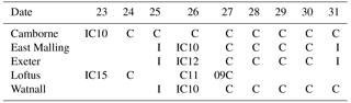
the Met Office Raman lidars located at Camborne (50∘12′ N, 5∘17′ W), East Malling (51∘17′ N, 0∘26′ E), Exeter (50∘43′ N, 3∘28′ W), Loftus (54∘31′ N, 0∘53′ W) and Watnall (53∘0′ N, 1∘15′ W) (Table 1 summarises the availability of data from these lidars for the period of this study);
-
twelve Lufft CHM 15 k ceilometers operated as part of the Met Office's UK ceilometer network.
Further details of these facilities are given in the Supplement.
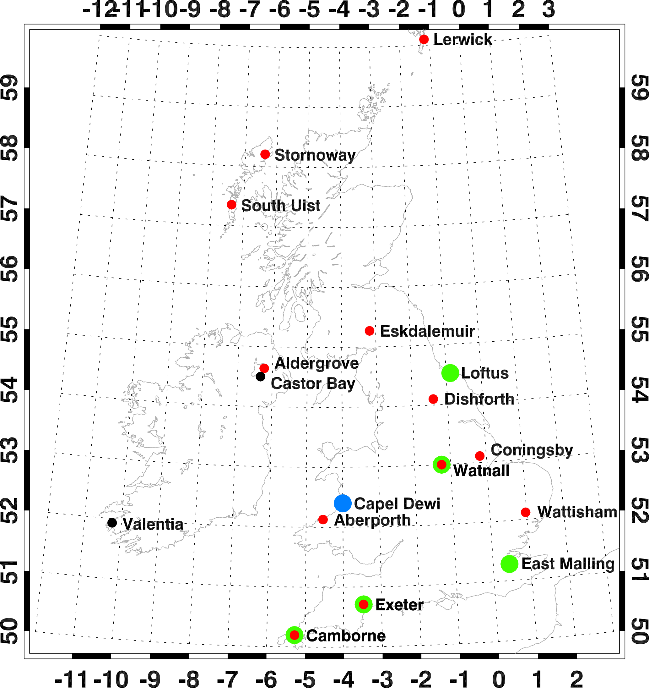
Figure 1Location of lidar stations used in this paper. Blue and green circles denote Raman lidars, red denotes Lufft CHM 15 k ceilometers and black denotes the two radiosonde stations mentioned in the text
Table 1Data coverage from Met Office lidars. I denotes intermittent coverage (1 h in 3), C denotes continuous coverage. IC10 denotes intermittent coverage up to 10:00 UTC, then continuous thereafter. C11 denotes no coverage up to 11:00 UTC, then continuous thereafter; 09C denotes continuous coverage up to 09:00 UTC and none thereafter.
The basic principles of the retrieval method are shown in the Supplement. Retrieval of the aerosol optical depth uses the N2 Raman signals and a nearby radiosonde profile. From the latter, a synthetic molecular-only scattering profile may be constructed and fitted to the measured profile in a region of the atmosphere free from aerosol, here taken to be 13–16 km. The ratio Ram(z) of the Raman to the molecular profiles then leads to curves such as that shown in blue in Fig. 2. In principle, this ratio can be inverted to give a profile of aerosol extinction coefficient, but this approach tends to lead to large random errors. Here we take advantage of the fact that for the episode under discussion the aerosol was distributed in very distinct layers, so a method was devised to calculate only layer-average or layer-total quantities. Figure 2 also shows R(z), the ratio of the elastic channel to the Raman channel, normalised to 1 between 13 and 16 km. Aerosols show up in this curve as departures from 1 (the molecular background), clearly showing the layered structure. (A small correction has been applied to R(z) to account for the difference between the Raman and Rayleigh scattering cross sections, using the radiosonde profile.) Such a structure was observed at all sites during the course of this event. We therefore calculate the integrated aerosol optical depth (AOD) across each layer:
where the overbars indicate that Ram(z) was averaged in the aerosol-free regions above and below each layer. Each lidar profile used here was examined separately to determine the layer altitudes and the width of the aerosol-free regions, which were chosen as far as possible to be at least 1 km deep.
As the photon-counting signals can be assumed to follow Poisson statistics, the precision error in AOD is readily calculated from the number of photon counts in the regions above and below each layer. A further source of error comes from the choice of radiosonde profile used to normalise PR(z). For stations like Camborne and Watnall, where co-located radiosondes were released, this error is small, but for the other stations it is not negligible. As an example, Fig. 3 shows the same lidar data as Fig. 2, but using a radiosonde from Camborne rather than Castor Bay (Fig. 1). The difference in AOD for the five layers is greater than the statistical uncertainty, showing that this source of error is important for free tropospheric aerosol measurements by Raman lidar.
Retrieval of the integrated aerosol backscatter (IAB) and hence the mean lidar ratio LR (LR = AOD/IAB) for each layer requires measurement of both polarisation components, and this was only possible for the Met Office Raymetrics lidars. Signals from the two elastic channels were added and used to generate an R(z) profile as before. The integral of B[R(z)−1]n(z) across each layer then gave IAB (Bates, 1984). Errors in IAB come from the Poisson statistics in both the signals in the layer and the background noise subtracted from the measured lidar signals, which are treated differently under the integral (variances being added for the signals and standard deviations for the background). Finally, the two errors are added in quadrature to give the error in IAB and LR calculated for each layer in the usual way.
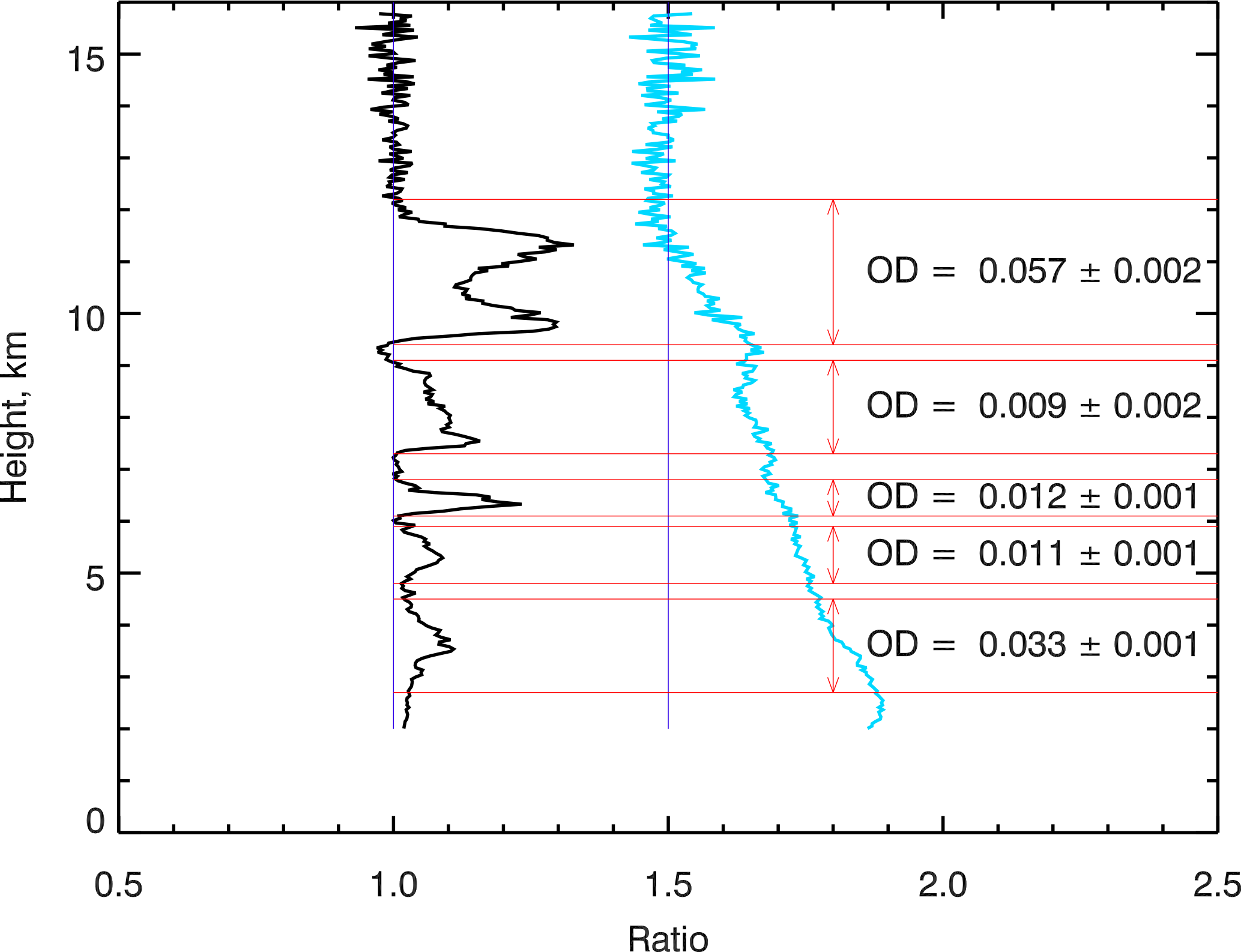
Figure 2Normalised ratios of elastic to Raman signals (black, normalised to 1) and synthetic to Raman molecular signals (blue, normalised to 1.5), using Capel Dewi lidar data from the night of 23–24 May 2016, between 21:49 and 03:09 UTC. The Castor Bay radiosonde profile for 00:00 UTC on 24 May 2016 was used for the molecular profile. Five distinct layers are identified, each by horizontal lines at their boundaries. The AOD is also shown for each layer.

To gain an appreciation of the extent and persistence of the aerosol, we first examine the ceilometer measurements since continuous coverage was available from all of them throughout the period, with aerosol measurements limited only by the presence of cloud.
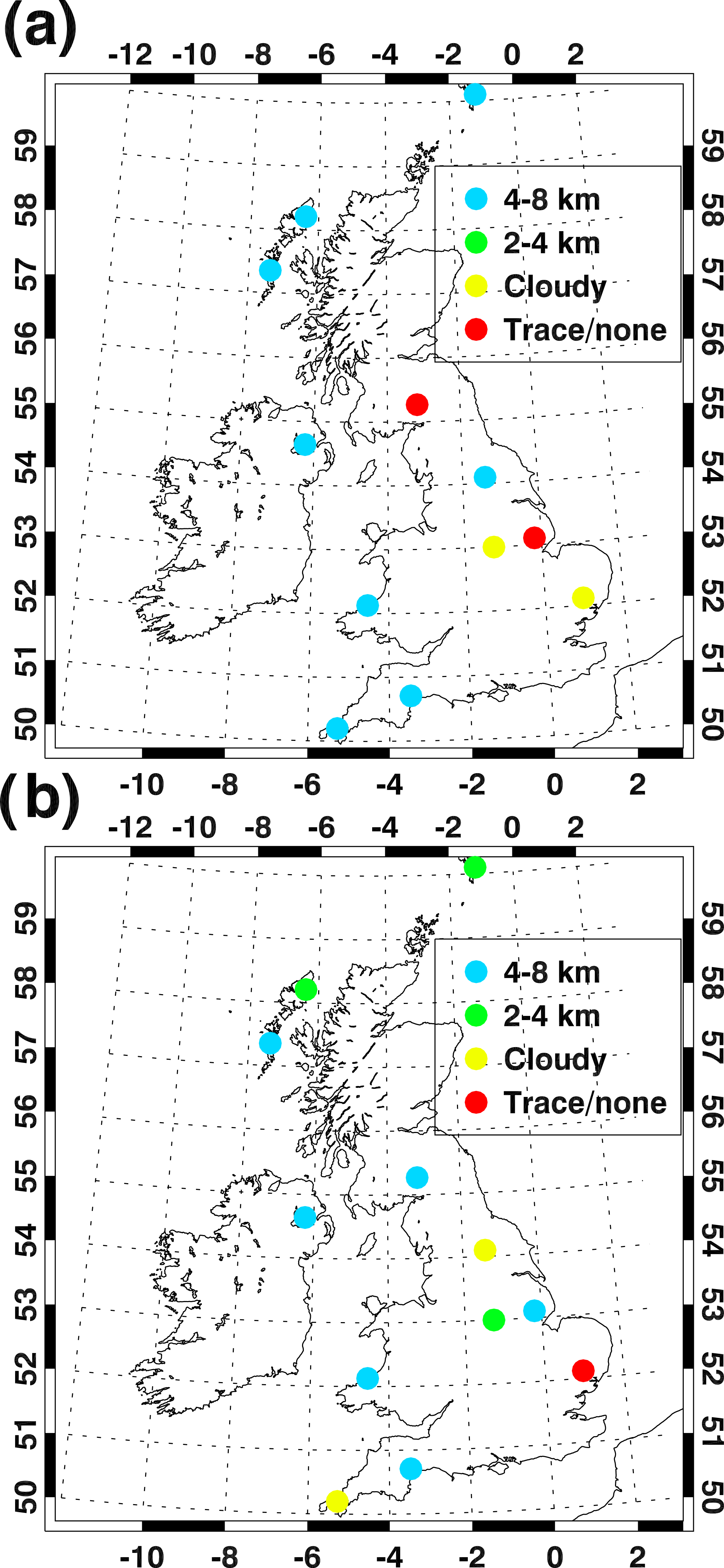
Thin layers of free-tropospheric aerosol began to appear over the UK during 22 May 2016 and persisted intermittently until the end of the month. As an example, Fig. 4 shows the variation of backscatter signal with height and time of the Lufft ceilometers at Lerwick (60∘8′ N, 1∘11′ W), Dishforth (54∘7′ N, 1∘24′ W) and Camborne (50∘12′ N, 5∘17′ W) on 23 May. Thin layers of enhanced backscatter due to aerosols are shown throughout the day at Camborne and from 10:00 UTC onwards at the other two stations. Similar patterns are seen in the layers at all three stations, suggesting that the aerosol layer was widespread over the UK during the second half of 23 May. To demonstrate this further, Fig. 5 summarises the ceilometer observations during 23 and 24 May. Four categories are shown: those with aerosol between 4 and 8 km (blue), those with aerosol between 2 and 4 km but no higher (green), those with no or only a trace of aerosol (red) and those where cloud cover precluded observations (yellow). High-altitude aerosol (>4 km) was indeed widespread across the UK on both days, with the suggestion of a clearance in the far north on 24 May.
To examine the duration of the event, the total number of ceilometers which observed definite aerosol layers, trace amounts or no aerosol, or were restricted by cloud cover, was plotted for each day from 22 to 27 May (Fig. 6). This plot shows that the event seems to have peaked in terms of coverage on 24 May, although the increasing cloud cover thereafter means that some aerosol is likely to have been missed. None of the ceilometers detected aerosol after 27 May, although continuing low cloud cover restricted observations to around half of the stations until clear skies returned on 5 June.
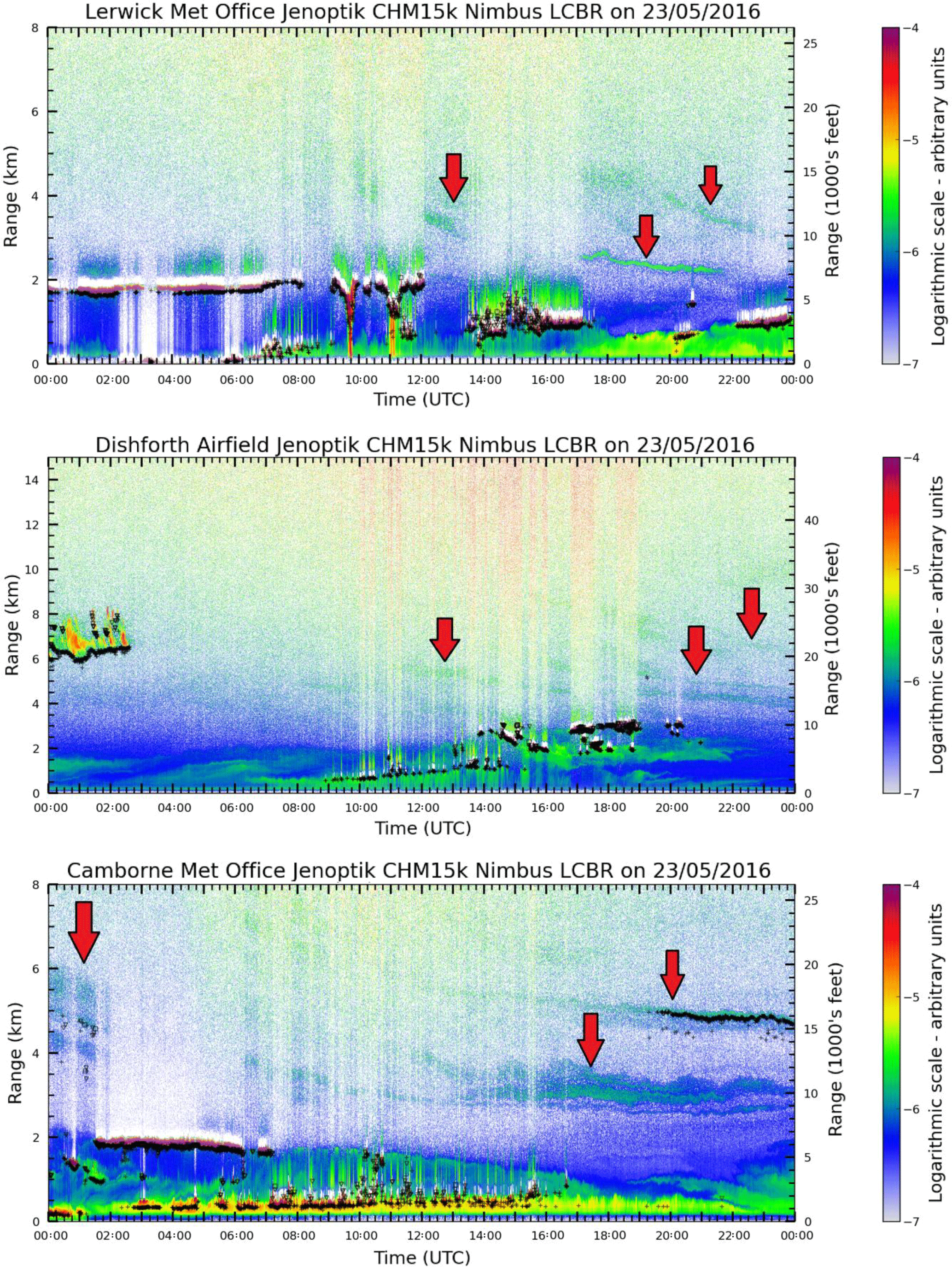
Figure 4Variation of backscatter signal with time and height over the course of 23 May 2016 at three Met Office stations. The black marks indicate cloud bases. The dark-blue and green layers above 2 km identified by the red arrows depict the aerosol layers.
The ceilometers only provide consistent measurements up to 8 km, and their infrared wavelength means they can only give qualitative information on the presence or not of aerosols. To extend the measurements to the tropopause and obtain quantitative information about the aerosol, we now turn to the Raman lidars. A qualitative inspection of the Met Office elastic channels (parallel and perpendicular polarisation) showed that there was extensive aerosol between 8 km and the tropopause, which was not captured by the ceilometers. This was observed at Camborne during 24–28 May, East Malling from 25 to 27 May, Exeter from 25 to 31 May and Watnall from 26 to 31 May. The Capel Dewi lidar also observed aerosol between 8 and 12 km up to the end of May. This shows that the event persisted from 22 to 31 May with aerosol layers found at all altitudes in the troposphere. We now concentrate on the night-time measurements from the Raman lidars to obtain quantitative information on these layers.
A similar analysis to that described in Sect. 3 was conducted for all the continuous night-time data collected by the Raman lidars between 23 and 31 May, after eliminating periods affected by cloud. Figure 7 shows the total aerosol optical depth above 2 km measured by the Raman lidars during this period, aggregated into whole-night averages. The greater sensitivity of these lidars means that aerosol was measured up to the night of 30–31 May at Capel Dewi with traces evident up to the same time at some of the other stations. However, the coverage is patchy due to the combination of intermittent sampling and low cloud cover.
The highest AOD measured was that at Capel Dewi on the night of 23–24 May, from the profile shown in Fig. 3. Although the value is sensitive to the choice of radiosonde profile, the total AOD of ∼0.13 above 2 km clearly results from aerosol observed throughout the free troposphere. All other AOD measurements at all the stations were below 0.1, with the values decreasing with time to below 0.05 after 28.
The evolution of lidar ratio as a function of optical depth is shown for the Met Office lidars in Figs. 8 and 9, for aerosol layers above and below 7 km respectively. Here, hourly average data are presented, as there could on occasion be considerable variability in AOD during a night; an example is 27–28 May at Camborne, where the total AOD varied between 0.02 and 0.09 over the 5 h measurement period. With the exception of a few outliers, the lidar ratios generally fall between 35 and 65 sr, consistent with the lidar ratios of 21–67 sr at 355 nm for Canadian and Siberian smoke reported by Müller et al. (2005) and with the values of 46±13 sr found in the 10-year study of forest fire smoke by Müller et al. (2007) using EARLINET data. There seems to be a greater spread of lidar ratios in the upper-tropospheric layers than in the mid-troposphere, where the spread is more like 40–60 sr. Note that the abscissa scales in Figs. 8 and 9 are different: most of the aerosol measured in this data set was found in the upper troposphere, where AOD values generally extended to 0.07, compared to 0.035 in the mid-troposphere.
The volume depolarisation ratio for the lidar profiles containing aerosol layers was a few percent at 355 nm, consistent with optically thin layers embedded within strong molecular backscatter. However, when converted to aerosol depolarisation ratios, δa, a remarkably consistent picture emerged across the different stations. Below 7 km, the value of δa was in the range 0.04–0.06, whereas above 7 km it was generally close to 0.20: for all four of the nights at Camborne and two of those at Watnall, δa lay in the range 0.18–0.21. Lower values were measured above 7 km at Exeter and East Malling on 25–26 May (0.15) and a high value at Watnall on 26–27 May (0.31) but the clear altitude difference remains. Values around 0.2 are consistent with those found at 355 nm by Burton et al. (2015) in aged smoke plumes, but the values around 0.05 are similar to the much lower δa values reported at 532 nm (Burton et al., 2015; Murayama et al., 2004). It is clear that δa at 355 nm for smoke particles can vary considerably.
A higher value of δa means the particles are more depolarising, which suggests more irregular solid shapes. As all the measurements here were made using the same laser wavelength, we cannot infer anything about particle size from the data, but the greater δa at higher altitudes is consistent with some of the smoke particles having acquired an ice coating at the colder temperatures near the tropopause – consistent with the ice-nucleating potential of smoke particles identified by Tan et al. (2014).
Having observed the presence of aerosol layers over the UK, three questions need to be answered. Where did they come from? How old are they? At what height(s) was the aerosol injected into the atmosphere?
Copernicus Atmospheric Monitoring Service (CAMS) daily fire products (available from http://macc.copernicus-atmosphere.eu/d/services/gac/nrt/fire_radiative_power, last access: 3 September 2016) showed extensive forest fires in Canada during May 2016, especially in Saskatchewan and Alberta (e.g. Fig. 10). Given the prevailing westerly winds at midlatitudes and the presence of deep convection over Canada capable of lifting the smoke, these provide the most likely source for the aerosol found over the UK. This hypothesis will now be examined using meteorological charts, trajectory calculations and satellite observations.
The air flow in the free troposphere impinging the UK on 20 May (Fig. 11a) was zonal, with rapid flow across the Atlantic around a trough at 54∘ N, 32∘ W. This provided a route to bring smoke aerosol across from Canada. After this, the pattern became more complicated. The trough moved steadily eastward and deepened, with its axis along the Irish Sea by 12:00 UTC on 22 May (Fig. 11b). At the same time, a deepening depression east of Newfoundland resulted in a second trough near 45∘ N, 40∘ W. These two troughs and the ridge in between set up an omega block on 23 May which resulted in a split jet stream, with one branch heading north over Iceland towards the Norwegian Sea and the other heading south across the Mediterranean (Fig. 11c). (An omega block is characterised by an upper–level ridge or anticyclone flanked by two cut-off lows or troughs, to the south-west and south-east.) As the block moved and distorted, the UK lay first under the eastern trough (06:00 UTC on 22 May to 12:00 UTC on 23 May), then the anticyclone (18:00 UTC on 23 May to 12:00 UTC on 24 May, Fig. 11c), the western cut-off low (18:00 UTC on 24 May to 00:00 UTC on 29 May, Fig. 11d) and finally a broad area of almost no flow which persisted until a second, weaker omega block was established on 30 May as another depression developed in the western Atlantic and moved eastwards (not shown). From 23 to 31 May therefore the flow over the UK was slack and variable, which meant that smoke transported in the zonal jet up to 22 May was able to remain in the vicinity of the UK.
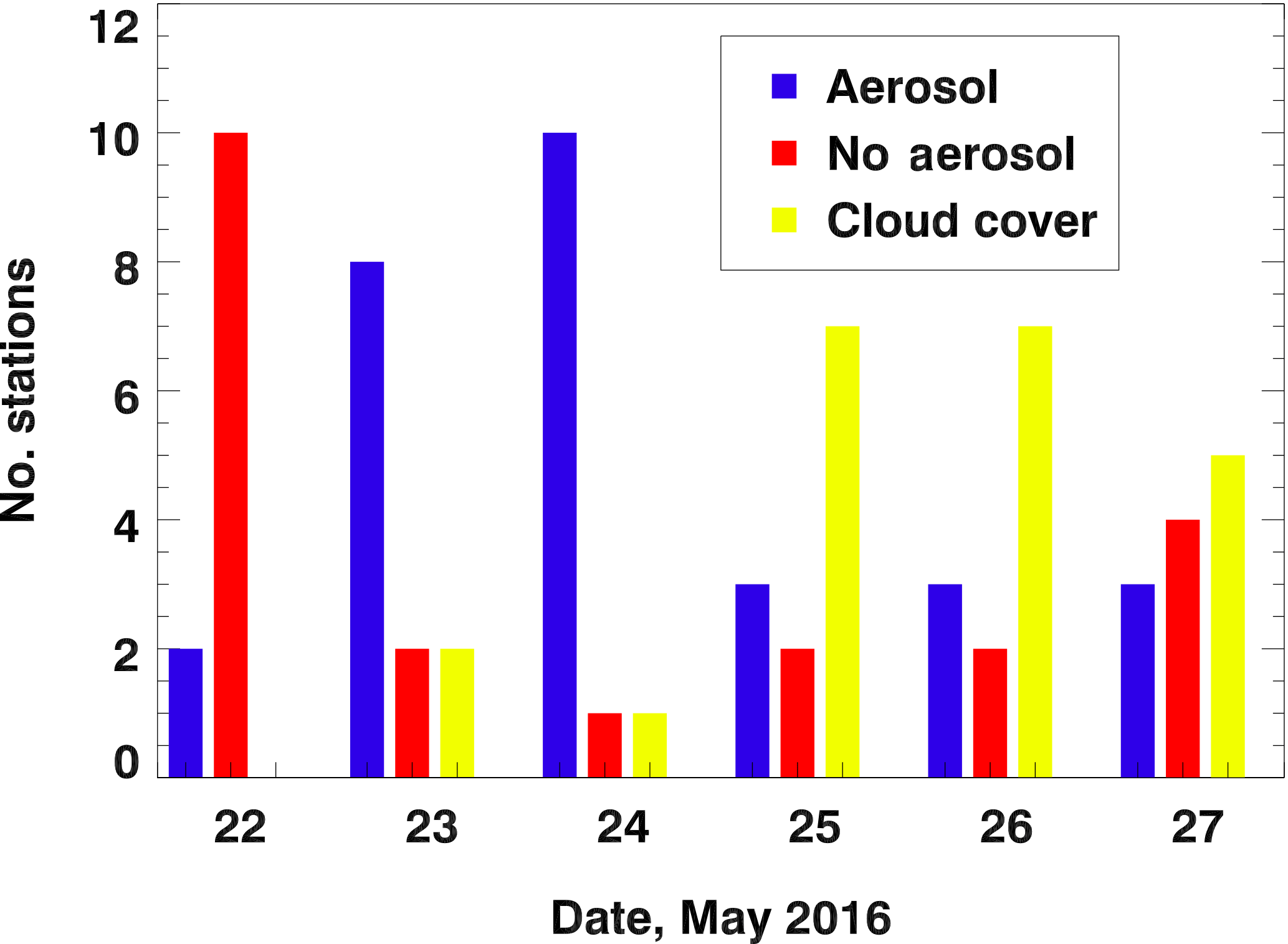
Figure 6The number of Lufft ceilometers that observed distinct layers of aerosol (blue), trace amounts or no aerosol (red), or were obscured by clouds (yellow) for the period 22 to 27 May 2016.

Figure 7Total aerosol optical depth measured above 2 km by the Raman lidars during the last 8 nights of May 2016, expressed as whole-night averages. The Capel Dewi points are those calculated using the Camborne radiosonde.
5.1 Air parcel trajectories
We now examine air parcel trajectories for evidence that the aerosol-laden air crossed the Atlantic from Canada. To be useful for this purpose, trajectories need to be non-dispersive – i.e. trajectories from nearby starting points need to follow a similar path. Unfortunately, this did not prove to be the case for most of this event, precluding any meaningful conclusion on air mass origin. Meteorological conditions with large horizontal flow separation, as is found upstream of a block, are known to introduce large uncertainty in trajectory calculations (Dacre and Harvey, 2018). We concentrate therefore on the period leading up to the start of the event when coherent sets of trajectories were found.
Trajectories were calculated using NOAA's HYSPLIT trajectory model (Draxler and Hess, 1998; Stein et al., 2015), both backward in time from the locations of the lidars and forward in time from locations in western Canada. A matrix of nine starting points was defined, spaced by 0.5∘ in latitude and longitude; low dispersion of these nine trajectories is required if the calculations are to be considered reliable.
Figure 8Lidar ratio plotted against total aerosol optical depth measured above 7 km by the Met Office Raman lidars on different nights.

Figure 9Lidar ratio plotted against total aerosol optical depth measured from 2 to 7 km by the Met Office Raman lidars on different nights.

Figure 10CAMS daily fire product for 17 May 2016. Colours show the average of the observed fire radiative power areal density in W m−2.

Figure 11Geopotential height (m) at 300 hPa for 20–26 May 2016 from NCEP–NCAR reanalyses (Kalnay et al., 1996), showing how the zonal flow developed into a blocking pattern.
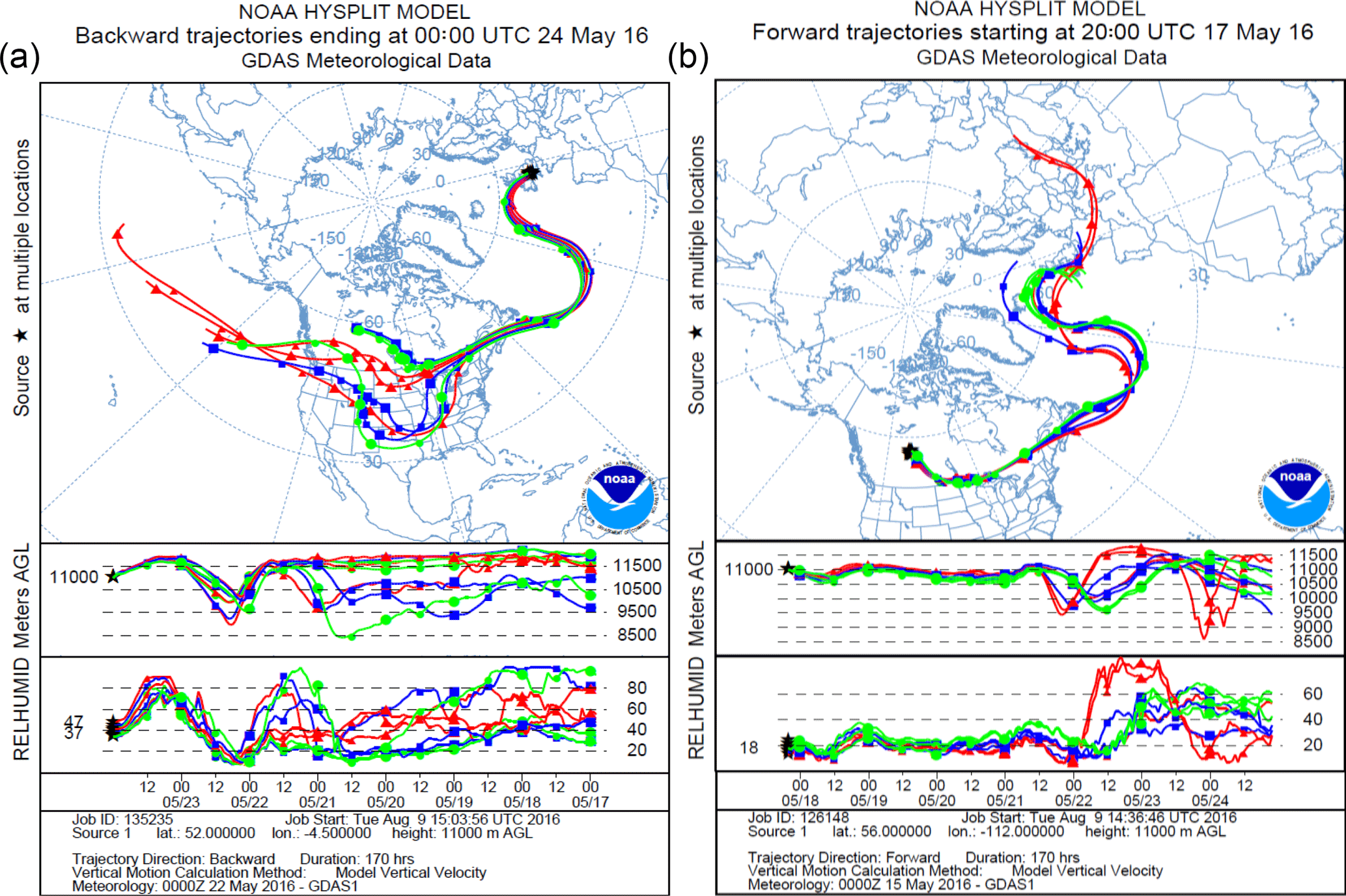
Figure 12Back trajectories calculated by HYSPLIT. (a) Nine back trajectories started at 11 km from a square 1∘ wide over Capel Dewi at 00:00 UTC 24 May 2016; (b) Nine forward-trajectories started at 11 km from a square 1∘ wide over 56.5∘ N, 111.5∘ W at 20:00 UTC 17 May 2016.
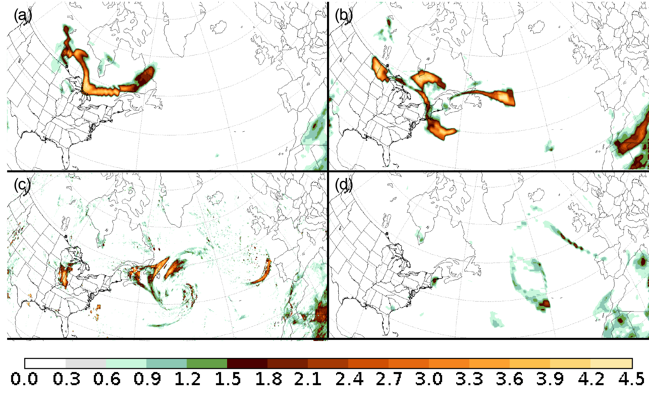
Figure 13OMPS Aerosol Index for sections of the S-NPP orbits at 05:00 UTC on (a) 19, (b) 20, (c) 21 and (d) 22 May. Images courtesy of Colin Seftor.
As an example, Fig. 12 (left panel) shows backwards trajectories from 11 km above Capel Dewi at 00:00 UTC on 24 May, corresponding to the lidar profile in Fig. 2. Also shown are the forward trajectories at the same height from above Fort McMurray (56.72∘ N, 111.38∘ W) at 20:00 UTC on 17 May, when cumulonimbi occurred over the fires. In both cases, the trajectories are sufficiently consistent to suggest that air passing over the UK on 23–24 May originated over the fire region of western Canada on 17.
However, examples like this proved rare. At other heights on 24 May, the back trajectories from Capel Dewi were too dispersive to reveal an air mass origin – by then the block was well set up with slack, incoherent flow. We therefore turn to satellite observations for evidence that the smoke crossed the Atlantic.
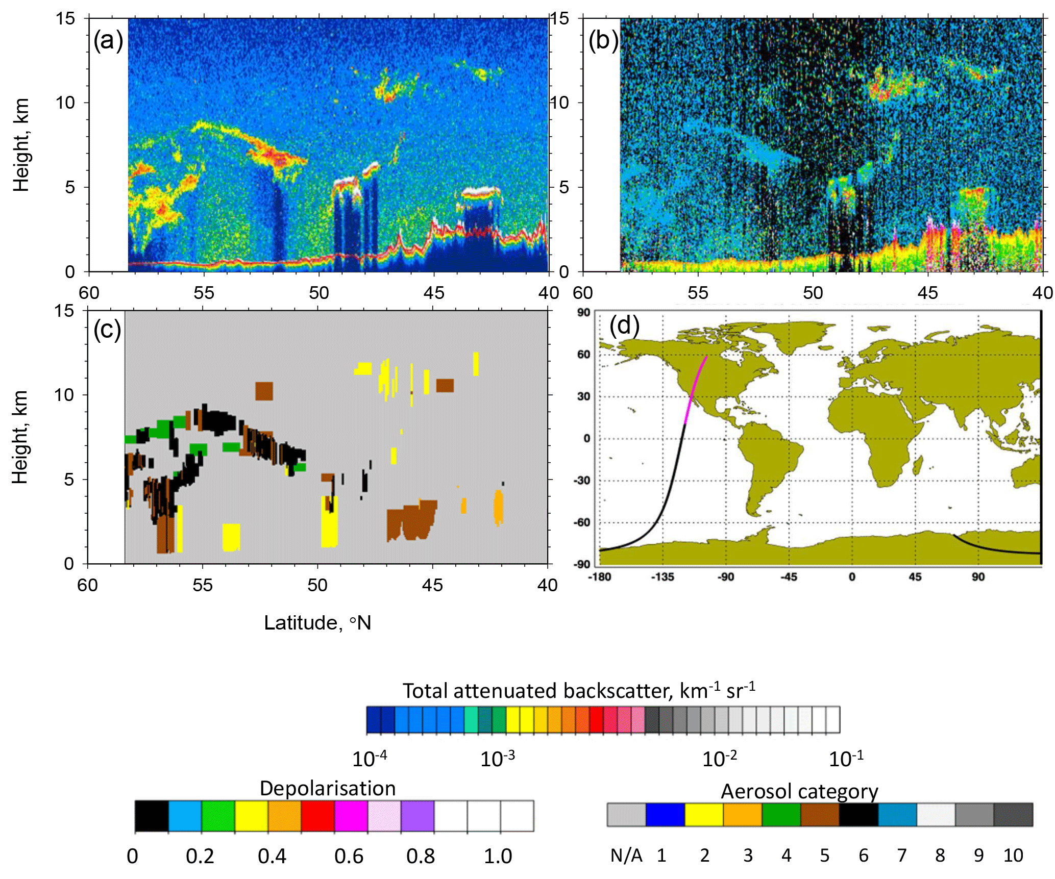
Figure 14(a) Total attenuated backscatter at 532 nm km−1 sr−1; (b) volume depolarisation ratio; (c) aerosol subtype plotted against position for (d) a section of the CALIPSO orbit (shown in pink) from 09:34 to 09:39 UTC on 18 May 2016. Figure adapted from online figures on the CALIPSO website. Colour bars for each panel have been expanded and are shown separately for clarity. Aerosol categories 5 (brown, polluted aerosol) and 6 (black, smoke) are of most interest to this study.
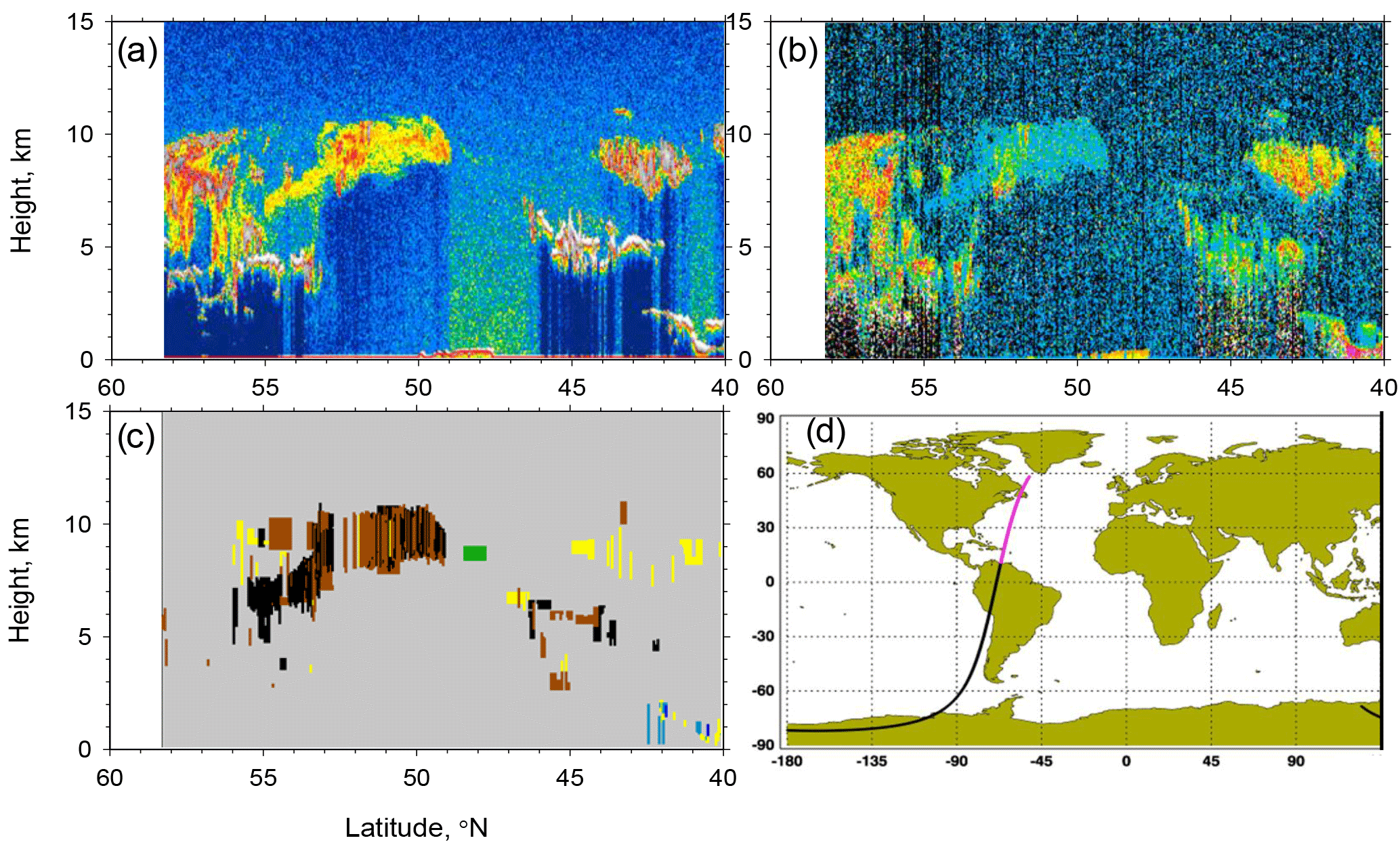
Figure 15As Fig. 14 for a section of the CALIPSO orbit which passed over the Atlantic from 06:04 to 06:09 UTC on 20 May 2016.
5.2 Satellite data
Several sources of data were used to track the smoke plume from Canada to the UK:
-
The CALIOP lidar on board the CALIPSO satellite measures backscatter at 532 and 1064 nm and depolarisation at 1064 nm (Winker et al., 2009). Plots of the data are available from http://www-calipso.larc.nasa.gov (last access: 31 July 2018): these include backscatter, volume depolarisation and various other derived products. Plots of the version 4.10 products are used in this study. As well as the aerosol classification provided by NASA, smoke is expected to display low depolarisation: Pereira et al. (2014) measured depolarisation values of 5 % or lower for forest fire smoke. This is consistent with the volume depolarisation of <6 % measured by the Raman lidars over the UK.
-
The CATS lidar aboard the International Space Station (ISS) is similar to CALIOP, with channels at 532 and 1064 nm. Data plots at http://cats.gsfc.nasa.gov/data/browse/ (last access: 31 July 2018) were examined for indications of smoke-like aerosol. Smoke was identified as aerosol which appears in the total backscatter but not in the perpendicular backscatter, again consistent with the weak volume depolarisation.
-
The Ozone Mapping Profiler Suite (OMPS) instrument on the SUOMI NPP satellite measures an Aerosol Index (AI) (Hsu et al., 1999), defined as the difference in the fraction of radiances, I, received at 331 and 360 nm to those calculated for a pure molecular atmosphere:
The AI is defined such that UV-absorbing aerosols have positive values proportional to AOD (Hsu et al., 1999). For the purpose of this article, the AI is used as a measure of the presence of aerosol and an approximate guide to the amount of it.
-
The SEVIRI instrument aboard the Meteosat-10 satellite provides a geostationary view of the Earth. Natural Colour RBG images provided by EUMETSAT were examined every 15 min from 03:00 UTC 22 May to 19:45 UTC 24 May. In these images, smoke appeared as a faint blue-grey colour and was most distinct just after dawn and just before dusk, when the scattering of sunlight towards the satellite from the small smoke particles was more prevalent. SEVIRI images from 22 to 23 May are shown in Fig. S2 in the Supplement.

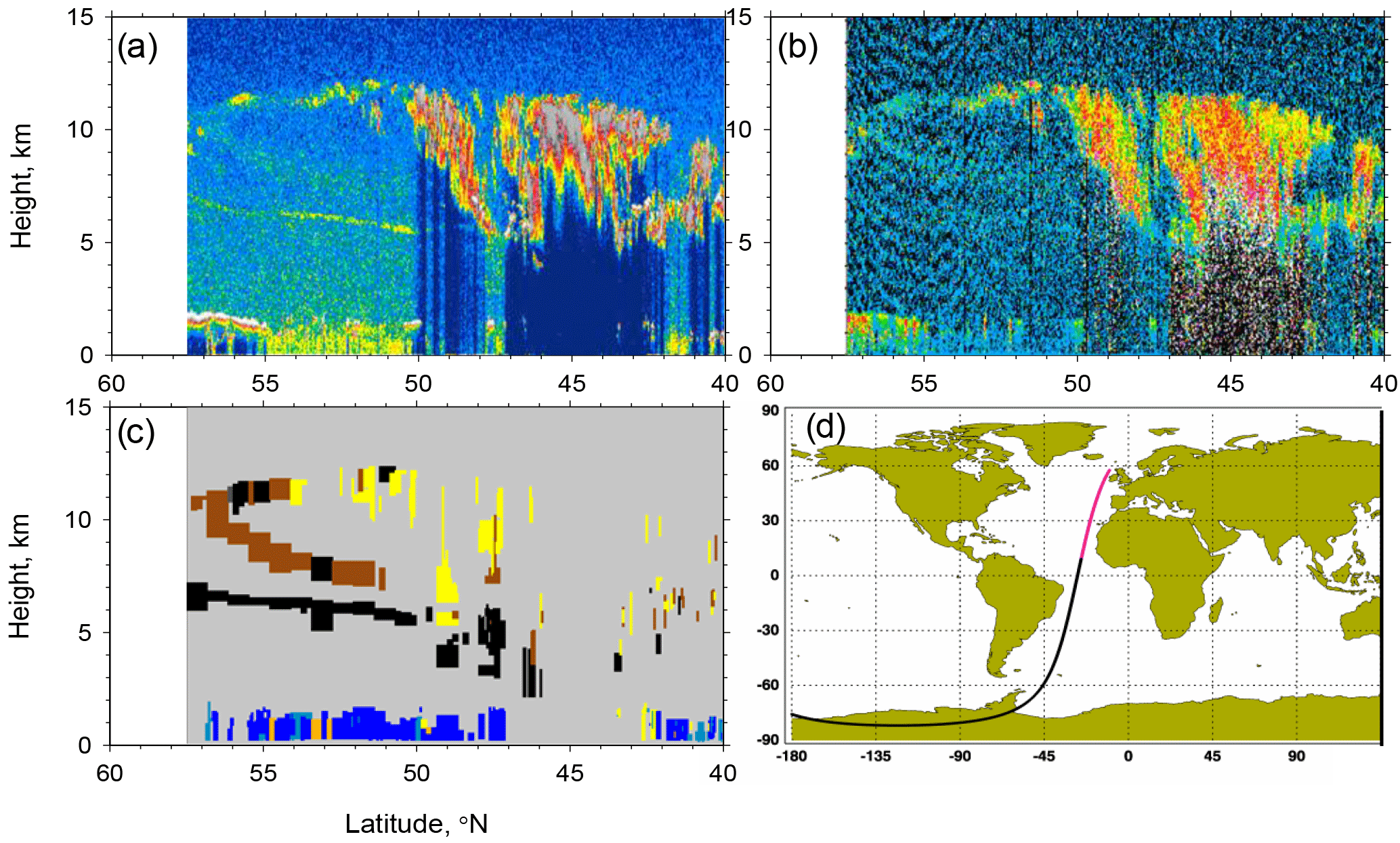
Figure 17The total attenuated backscatter (a) and perpendicularly polarised backscatter (b) signals from the CATS lidar around 02:16 on 22 May, adapted from figures on the CATS website. Colours are the same as CALIPSO (Fig. 14). Also shown is the path of the ISS and (in green) where the measurements were taken (c).
The eastward transport of aerosol across North America and over the Atlantic Ocean in Fig. 12 is shown by the OMPS-AI measurements (Fig. 13). The broad shape of the smoke plume heading eastward from Alberta is consistent with the HYSPLIT trajectories shown in Fig. 12 and shows aerosol reaching the western Atlantic on 20 May. Thereafter, the smoke progresses eastward towards Europe, with a strip of elevated aerosol index lying west of Ireland by 05:00 UTC on 22 May. Evident in this figure is the apparent thinning of the aerosol layer as it traverses the Atlantic. In fact, a more complex evolution was taking place, eventually leading to the multiple-layered structure shown in Fig. 3. The key to this may be seen in Fig. 13c, which shows the aerosol being entrained into the low-pressure system developing east of Newfoundland on 21 May. Differential advection by the ambient wind shear is a feature of flow around a cyclone, in this case causing the initially coherent blob of aerosol to be stretched and distorted, forming the multi-layered structures observed over the UK. To show how this evolution occurred we now turn to space-borne lidar data, which are capable of distinguishing features in the vertical profiles of the aerosol.
Figure 14 shows backscatter, depolarisation and aerosol characterisation between 09:34 and 09:39 UTC on 18 May 2016 from a CALIOP orbit passing near 104∘ W, around 400 km east of Fort McMurray. CALIOP identified smoke between 3 and 8 km at the northernmost end of the orbital section, where aerosol depolarisation was <10 %. On the previous orbit, at ∼ 08:00 UTC roughly along 80∘ W between 53.5 and 58∘ N, smoke was also present, again between 3 and 8 km, but none of the orbits further east observed smoke on this day. By 20, an orbit along ∼57∘ W around 06:05 UTC measured mixed smoke and polluted aerosol from 49 to 56∘ N between 5 and 11 km (Fig. 15). Extensive smoke was also observed between 4 and 11 km on 21 May north of 49∘ N along ∼40∘ W and on 22 May north of 50∘ N along ∼30∘ W (not shown). By the early hours of the 23 May, smoke layers had reached the vicinity of the UK (Fig. 16), again being consistent with the trajectories.
The presence of smoke across the Atlantic Ocean is best shown by the total and perpendicular backscatter measurements by the CATS lidar in the early hours of 22 May (Fig. 17). Optically thin aerosol is identified as the light-blue layers in the total backscatter plot and further classified as smoke by the lack of such layers in the perpendicularly polarised signal. Figure 17 shows that by 22 May the smoke plume extended from 55 to 15∘ W and was present from the top of the boundary layer to above 10 km. As noted previously, the smoke aerosol now exhibited multiple thin layers due to the stirring effect of differential advection as the air mass travelled eastward.
The combination of CALIPSO and CATS space-borne lidar, together with OMPS, therefore shows that a plume of smoke was drawn from Canada between 17 and 20 May, which was transported eastward by the zonal flow during this period. Later, as the flow became blocked, this smoke was becalmed over the UK and was observed by the UK lidar network; smoke also appeared as thin streaks in SEVIRI images of the UK, as shown in the Supplement. We have therefore shown that the aerosol observed by the Raman lidar at Capel Dewi and Met Office lidar network on 23 and 24 May had a consistent origin from the Canadian forest fires in western and central Canada around 17 May. This gives the smoke a 6–8-day transport time.
This study has presented observations of free-tropospheric aerosols by ceilometers and Raman lidars over the UK from 23 to 31 May 2016 and examined the origin of the aerosol. The principal conclusions are as follows.
-
Ceilometer measurements showed that much of the United Kingdom was covered by free-tropospheric smoke layers on 23 and 24 May.
-
Raman lidar observations showed that the smoke was found throughout the troposphere, but with greatest optical depth above 7 km.
-
The maximum optical depth measured was ∼0.15 with most values between 0.1 and 0.05: these values diminished with time throughout the event.
-
The properties of the aerosol as determined from Raman lidar were consistent with those of smoke from forest fires: low volume depolarisation (<6 % and a lidar ratio in the range 35–65 sr).
-
Particle depolarisation ratios showed a marked difference with height – below 7 km the values were around 0.05, consistent with previous measurements at 532 nm, but above 7 km the ratios were around 0.2, closer to previous measurements at 355 nm. This indicates that the nature of the smoke particles was different above and below 7 km.
-
The smoke lingered over western Europe for 9 days due to an atmospheric block which prevented eastward advection.
-
Although trajectory calculations proved indecisive for identifying the origin of the smoke, analysis of satellite lidar observations showed how the plume was drawn out over the Atlantic during 17–21 May before becoming becalmed by the block that developed on 22 May.
The study shows the value of combining different kinds of lidars in following the evolution of long-range smoke transport events, since the 24 h capability of ceilometers allows maximum use to be made of breaks in cloud cover, while the quantitative information available from Raman lidars yields information on particle properties. The study shows how a smoke plume from Canadian wildfires was drawn into a pattern of thin layers far downstream of its source, due to stirring of the atmosphere by flow around a cyclone in the mid-Atlantic, and how these layers could be exploited in the lidar data analysis to produce robust estimates of particle properties. The study also shows how atmospheric blocking resulted in a smoke event remaining over the UK for over a week, during which time the layers became optically thinner but no change was observed in particle properties.
Data from the Capel Dewi lidar may be accessed from https://doi.org/10.17632/vg93bvf48h.1 (Vaughan, 2018).
Data for the Met Office Ceilometers and lidars are available from http://catalogue.ceda.ac.uk/uuid/38a6e76871fca4c58d0f831e532bff41 (Met Office, 2015).
The supplement related to this article is available online at: https://doi.org/10.5194/acp-18-11375-2018-supplement.
Data for the paper were collected by MA, JS and DPW. Data analysis was performed by APD, HMAR and GV and the manuscript written by APD, GV and DMS. The project was led by GV.
The authors declare that they have no conflict of interest.
We thank the following individuals and organisations for providing access to
data and imagery: Colin Seftor (NASA) for producing the OMPS-AI plots in
Fig. 13, the Centre for Environmental Data Analysis (CEDA) and the
Met Office for providing access to the Met Office LIDARNET data, the
Department for Transport and the Civil Aviation authority for funding the Met
Office Raman Lidar network, EUMETSAT for providing the analysis of SEVIRI
data, the NASA CALIOP and CATS teams for providing access to plots on the
Web. Funding for Adam P. Draude was provided by the UK Natural Environment Research
Council through Manchester–Liverpool Doctoral Training Programme grant
NE/L002469/1. Partial funding for Geraint Vaughan and David M. Schultz was provided by the
Natural Environment Research Council to the University of Manchester through
grant NE/I005234/1.
Edited by: Jui-Yuan Christine Chiu
Reviewed by: two anonymous referees
Alados-Arboledas, L., Mueller, D., Guerrero-Rascado, J. L., Navas-Guzman, F., Perez-Ramirez, D., and Olmo, F. J.: Optical and microphysical properties of fresh biomass burning aerosol retrieved by Raman lidar, and star-and sun-photometry, Geophys. Res. Lett., 38, L01807, https://doi.org/10.1029/2010GL045999, 2011. a
Amiridis, V., Balis, D. S., Giannakaki, E., Stohl, A., Kazadzis, S., Koukouli, M. E., and Zanis, P.: Optical characteristics of biomass burning aerosols over Southeastern Europe determined from UV-Raman lidar measurements, Atmos. Chem. Phys., 9, 2431–2440, https://doi.org/10.5194/acp-9-2431-2009, 2009. a
Ansmann, A., Baars, H., Tesche, M., Müller, D., Althausen, D., Engelmann, R., Pauliquevis, T., and Artaxo, P.: Dust and smoke transport from Africa to South America: Lidar profiling over Cape Verde and the Amazon rainforest, Geophys. Res. Lett., 36, L11802, https://doi.org/10.1029/2009GL037923, 2009. a
Bates, D.: Rayleigh scattering by air, Planet. Space Sci., 32, 785–790, https://doi.org/10.1016/0032-0633(84)90102-8, 1984. a
Burton, S. P., Hair, J. W., Kahnert, M., Ferrare, R. A., Hostetler, C. A., Cook, A. L., Harper, D. B., Berkoff, T. A., Seaman, S. T., Collins, J. E., Fenn, M. A., and Rogers, R. R.: Observations of the spectral dependence of linear particle depolarization ratio of aerosols using NASA Langley airborne High Spectral Resolution Lidar, Atmos. Chem. Phys., 15, 13453–13473, https://doi.org/10.5194/acp-15-13453-2015, 2015. a, b, c
Dacre, H. F. and Harvey, N. J.: Characterizing the Atmospheric Conditions Leading to Large Error Growth in Volcanic Ash Cloud Forecasts, J. Appl. Meteorol. Clim., 57, 1011–1019, https://doi.org/10.1175/JAMC-D-17-0298.1, 2018. a
Damoah, R., Spichtinger, N., Forster, C., James, P., Mattis, I., Wandinger, U., Beirle, S., Wagner, T., and Stohl, A.: Around the world in 17 days – hemispheric-scale transport of forest fire smoke from Russia in May 2003, Atmos. Chem. Phys., 4, 1311–1321, https://doi.org/10.5194/acp-4-1311-2004, 2004. a
Draxler, R. R. and Hess, G. D.: An overview of the HYSPLIT_4 modeling system for trajectories, dispersion, and deposition, Aust. Meteorol. Mag., 47, 295–308, 1998. a
Forster, C., Wandinger, U., Wotawa, G., James, P., Mattis, I., Althausen, D., Simmonds, P., O'Doherty, S., Jennings, S. G., Kleefeld, C., Schneider, J., Trickl, T., Kreipl, S., Jäger, H., and Stohl, A.: Transport of boreal forest fire emissions from Canada to Europe, J. Geophys. Res., 106, 22887–22906, https://doi.org/10.1029/2001JD900115, 2001. a
Fromm, M.: Pyro-cumulonimbus injection of smoke to the stratosphere: Observations and impact of a super blowup in northwestern Canada on 3–4 August 1998, J. Geophys. Res., 110, D08205, https://doi.org/10.1029/2004JD005350, 2005. a
Giannakaki, E., Balis, D. S., Amiridis, V., and Zerefos, C.: Optical properties of different aerosol types: seven years of combined Raman-elastic backscatter lidar measurements in Thessaloniki, Greece, Atmos. Meas. Tech., 3, 569–578, https://doi.org/10.5194/amt-3-569-2010, 2010. a
Hsu, N. C., Herman, J. R., Torres, O., Holben, B. N., Tanre, D., Eck, T. F., Smirnov, A., Chatenet, B., and Lavenu, F.: Comparisons of the TOMS aerosol index with Sun-photometer aerosol optical thickness: Results and applications, J. Geophys. Res., 104, 6269–6279, https://doi.org/10.1029/1998JD200086, 1999. a, b
Kalnay, E., Kanamitsu, M., Kistler, R., Collins, W., Deaven, D., Gandin, L., Iredell, M., Saha, S., White, G., Woollen, J., Zhu, Y., Leetmaa, A., Reynolds, R., Chelliah, M., Ebisuzaki, W., Higgins, W., Janowiak, J., Mo, K. C., Ropelewski, C., Wang, J., Jenne, R., and Joseph, D.: The NCEP/NCAR 40-Year Reanalysis Project, B. Am. Meteorol. Soc., 77, 437–471, https://doi.org/10.1175/1520-0477(1996)077<0437:TNYRP>2.0.CO;2, 1996. a
Mattis, I., Ansmann, A., Wandinger, U., and Muller, D.: Unexpectedly high aerosol load in the free troposphere over central Europe in spring/summer 2003, Geophys. Res. Lett., 30, 2178, https://doi.org/10.1029/2003GL018442, 2003. a
Mattis, I., Mueller, D., Ansmann, A., Wandinger, U., Preissler, J., Seifert, P., and Tesche, M.: Ten years of multiwavelength Raman lidar observations of free-tropospheric aerosol layers over central Europe: Geometrical properties and annual cycle, J. Geophys. Res., 113, D20202, https://doi.org/10.1029/2007JD009636, 2008. a
Met Office: Met Office LIDARNET ceilometer network cloud base and backscatter data, available at: http://catalogue.ceda.ac.uk/uuid/38a6e76871fca4c58d0f831e532bff41 (last access: June 2016), 2015.
Müller, D., Mattis, I., Wandinger, U., Ansmann, A., Althausen, D., and Stohl, A.: Raman lidar observations of aged Siberian and Canadian forest fire smoke in the free troposphere over Germany in 2003: Microphysical particle characterization, J. Geophys. Res., 110, D17201, https://doi.org/10.1029/2004JD005756, 2005. a, b
Müller, D., Ansmann, A., Mattis, I., Tesche, M., Wandinger, U., Althausen, D., and Pisani, G.: Aerosol-type-dependent lidar ratios observed with Raman lidar, J. Geophys. Res., 112, D16202, https://doi.org/10.1029/2006JD008292, 2007. a, b, c
Murayama, T., Muller, D., Wada, K., Shimizu, A., Sekiguchi, M., and Tsukamoto, T.: Characterization of Asian dust and Siberian smoke with multiwavelength Raman lidar over Tokyo, Japan in spring 2003, Geophys. Res. Lett., 31, L23103, https://doi.org/10.1029/2004GL021105, 2004. a, b
Pereira, S. N., Preissler, J., Guerrero-Rascado, J. L., Silva, A. M., and Wagner, F.: Forest Fire Smoke Layers Observed in the Free Troposphere over Portugal with a Multiwavelength Raman Lidar: Optical and Microphysical Properties, Sci. World J., 2014, 421838, https://doi.org/10.1155/2014/421838, 2014. a, b, c
Sitnov, S. A. and Mokhov, I. I.: Anomalous transboundary transport of the products of biomass burning from North American wildfires to Northern Eurasia, Dokl. Earth Sci., 475, 832–835, https://doi.org/10.1134/S1028334X17070261, 2017. a
Stein, A. F., Draxler, R. R., Rolph, G. D., Stunder, B. J. B., Cohen, M. D., and Ngan, F.: NOAA's HYSPLIT Atmospheric Transport and Dispersion Modeling System, B. Am. Meteorol. Soc., 96, 2059–2077, https://doi.org/10.1175/BAMS-D-14-00110.1, 2015. a
Tan, I., Storelvmo, T., and Choi, Y.-S.: Spaceborne lidar observations of the ice-nucleating potential of dust, polluted dust, and smoke aerosols in mixed-phase clouds, J. Geophys. Res., 119, 6653–6665, https://doi.org/10.1002/2013JD021333, 2014. a
Vaughan, G.: Raman lidar data from Capel Dewi, 23–30 May 2016, https://doi.org/10.17632/vg93bvf48h.1, 2018.
Veselovskii, I., Whiteman, D. N., Korenskiy, M., Suvorina, A., Kolgotin, A., Lyapustin, A., Wang, Y., Chin, M., Bian, H., Kucsera, T. L., Pérez-Ramírez, D., and Holben, B.: Characterization of forest fire smoke event near Washington, DC in summer 2013 with multi-wavelength lidar, Atmos. Chem. Phys., 15, 1647–1660, https://doi.org/10.5194/acp-15-1647-2015, 2015. a
Wandinger, U., Muller, D., Bockmann, C., Althausen, D., Matthias, V., Bosenberg, J., Weiss, V., Fiebig, M., Wendisch, M., Stohl, A., and Ansmann, A.: Optical and microphysical characterization of biomass-burning and industrial-pollution aerosols from multiwavelength lidar and aircraft measurements, J. Geophys. Res., 107, 8125, https://doi.org/10.1029/2000JD000202, 2002. a
Weber, M. G. and Stocks, B. J.: Forest fires and sustainability in the boreal forests of Canada, Ambio, 27, 545–550, 1998. a
Winker, D. M., Vaughan, M. A., Omar, A., Hu, Y., Powell, K. A., Liu, Z., Hunt, W. H., and Young, S. A.: Overview of the CALIPSO Mission and CALIOP Data Processing Algorithms, J. Atmos. Ocean. Tech., 26, 2310–2323, https://doi.org/10.1175/2009JTECHA1281.1, 2009. a
Wooster, M. J. and Zhang, Y. H.: Boreal forest fires burn less intensely in Russia than in North America, Geophys. Res. Lett., 31, L20505, https://doi.org/10.1029/2004GL020805, 2004. a
The requested paper has a corresponding corrigendum published. Please read the corrigendum first before downloading the article.
- Article
(8576 KB) - Full-text XML
- Corrigendum
-
Supplement
(815 KB) - BibTeX
- EndNote